2.1. Facility and arrangement

The experiments were conducted in the $10^{\prime}\times 5^{\prime}$ closed-loop wind tunnel at the Department of Aeronautics at Imperial College, London. The wind tunnel test section is nominally 3.048 m wide $\times 1.524\ {\rm m}$ high ($10^\prime\times 5^\prime$) and 20 m long. Both the wind tunnel speed and air temperature are closed-loop controlled. The test models comprised a three-bladed rotor and two porous discs of different diameters with similar porosity designed to provide a similar resistance of the rotor at the tip-speed ratio of the tests. Both the rotor and discs were aligned normal to the flow. Throughout each test the actuator conditions were fixed, thus simulating below rated conditions for a horizontal axis wind turbine for which this normally applies.

The models were first tested in a nominally clean uniform flow of the wind tunnel test section in a $10\ {\rm m}\ {\rm s}^{-1}$ wind speed that served to establish their mean characteristics. Subsequent tests were conducted in two different turbulent flow regimes: (1) a $1:400$ scaled, simulated turbulent ABL with a mean hub height wind speed of $10\ {\rm m}\ {\rm s}^{-1}$; and (2) a uniform mean flow, $10\ {\rm m}\ {\rm s}^{-1}$ of homogeneous, small-scale, turbulence generated by a planar square mesh grid $(M=125\ {\rm mm})$. The ABL was designed according to the Engineering Sciences Data Unit (ESDU) method (ESDU82026 2002) assuming neutral conditions. A roughness length of $z_0 = 0.01\ {\rm m}$ was adopted from which the mean wind speed and streamwise intensity profiles were obtained. A boundary layer with similar characteristics was generated in the wind tunnel using Counihan spires (Counihan Reference Counihan1969) and a fence, and developed over a 15 m rough floor fetch. Figure 1 shows that despite a slightly weaker near-surface mean shear compared with the ESDU profiles, there is a good match in the wind tunnel for the mean velocity and intensity profiles across the rotor plane. The distribution of the ESDU values of the von Kármán length scale, which quantifies the scale of the largest eddies in the flow, varied significantly (Han et al. Reference Han, McCann, Mücke and Freudenreich2014) in response to small changes in $z_0$. At the planned rotor hub height of 150 m ($375\ {\rm mm}$), the length scale ranged between 140 m and 320 m. In the wind tunnel the von Kármán length scale was measured as 0.41 m, which is equivalent to 164 m at full scale. Figure 2 shows the wind tunnel set-up for these experiments, comprising the spires, fence and roughness fetch, and a biplanar grid (shown outside the wind tunnel) that replaced the Counihan arrangement for the tests in grid generated turbulence.

Figure 1.

Vertical profiles of the mean velocity (a) and streamwise turbulence intensity (b). The circular symbols denote hot-wire data acquired in the wind tunnel for the installed fetch. The ESDU values for $z_0 =0.01$ m at full scale are shown by the solid red line, with the dashed lines corresponding to the ${\pm }10\,\%$ limits. The dashed horizontal line at $Z=375\ {\rm mm}$ (150 m at full scale) represents the hub height for the rotor and porous discs. Both figures have a left wind tunnel scale axis and a right full scales axis, assuming $1:400$ scaling.

Figure 2.

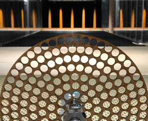
Set-up of the wind tunnel experiments. (a) The Counihan spires, fence and the ground roughness fetch are shown in the background. The rotor rig, comprising torque and r.p.m. sensors, electromagnetic brake and forward-reaching shaft are in the foreground. The large porous disc is seen mounted onto the shaft, which for this case, was locked from rotating. Shown outside the wind tunnel, on the right of the image, is a two-dimensional turbulence generation grid, which replaced the spires, fence and roughness when the grid turbulence experiments were conducted. Immediately ahead of the porous disc, the vertical hot-wire probe holder, with a right-angle hot-wire probe, is shown mounted on a linear rail, which enabled the distance between the sensor and the model (rotor or disc) to be varied. The general sign convention is shown. (b) End and front views of the rig with the large porous disc, showing the sign convention and origins. Here $x = 0$ lies at the streamwise location of the upstream face of the porous disc for the disc measurements, or at the streamwise location of the blade quarter chord for the rotor measurements; $Z = 0$ lies on the tunnel roughness floor for coordinates related to the ABL; $z=0$ lies at the centre of the porous plate or rotor. For two-point velocity correlations, the main hot wire was held at hub height, and a second hot wire was introduced, traversing vertically (shown in the end view) or transversally (shown in the front view) relative to the first wire, with separation $\Delta z$ or $\Delta y$. (c) The rotor and two porous plates used in these experiments. The central grey region on the porous plates shows the extent of the hub.

For the experiments in the ABL, all the models were tested in the same position in the wind tunnel. This was around 15 m downstream of the spires, at mid-width of the test section, and at an effective hub height of $375\ {\rm mm}$ (equivalent to 150 m at full scale). A right-angle hot-wire probe was mounted on a probe holder, with the sensor at hub height. The circular stem of the probe was approximately $2\ {\rm mm}$ in diameter and about $50\ {\rm mm}$ long, while the probe holder was approximately $4\ {\rm mm}$ in diameter and about $200\ {\rm mm}$ long. As such, it was assumed to have minimal effect on the mean and turbulent flow at the measured point. The probe was able to translate along $x$, at hub height, by means of a rail mounted on the floor upstream of the rotor rig.

For the experiments behind the grid, the models were mounted such that the hub was at the mid-width and mid-height of the test section. The right-angle hot-wire probe, on its probe holder, was at hub height and fixed at 12.5$M$. The rotor rig was able to translate downstream of the fixed hot-wire sensor.

The geometric blockage ratio based on the frontal area of the models in the wind tunnel working section was $4.3\,\%$ for the rotor, and $3.5\,\%$ and $1.0\,\%$ for the large and small porous discs, respectively. The upstream wind speed at hub height was measured with a Pitot-static probe and a Furness FCO560 micromanometer, with the latter also recording the wind temperature and atmospheric pressure. For the tests in grid turbulence, the Pitot probe was placed upstream of the grid. For the ABL experiments, it was $3.5D$ ahead and $2.5D$ to the side from the centres of the test models.

2.2. Porous discs and rotor

Figure 2 shows a schematic of models of the porous discs and the $D=500\ {\rm mm}$ diameter three-bladed turbine. The two porous discs were of $D=450\ {\rm mm}$ and $245\ {\rm mm}$ and fabricated from $4\ {\rm mm}$ thick medium-density fibreboard. In both discs, $12\ {\rm mm}$ diameter holes were spaced equidistant both radially and azimuthally. The ratio of the open area to total area for the small disc was 52.9 %. This ratio was slightly larger for the larger disc, 55.5 %, due to the smaller distance between the outermost array of holes and the disc perimeter.

The turbine was designed using conventional blade element momentum theory. The spanwise chord length and twist angle distributions were based on a design tip-speed ratio of $\varLambda =4.0$. The low Reynolds number SG6051, SG6043 and SD2030 airofoil sections (Selig, Donovan & Fraser Reference Selig, Donovan and Fraser1989; Giguère & Selig Reference Giguère and Selig1998) were blended along the blade span outward from the $42\ {\rm mm}$ diameter hub. The Reynolds numbers of the large and small porous discs, based on the wind speed at hub height and their diameters, were $3\times 10^{5}$ and $1.63\times 10^{5}$, respectively. The Reynolds number of the rotor, based on the tangential velocity and the chord at $0.75R$ (where $R=D/2$), was $6.35\times 10^{4}$.

For the hot-wire velocity measurements upstream of the rotor and discs, the models were mounted on a rig comprising an in-line Magtrol torque-r.p.m (revolutions per minute) sensor and a Magtrol proportional–integral–derivative (PID) controlled electromagnetic brake. For the rotor case, this was used to provide a constant rotational speed of 1500 r.p.m., equivalent to a tip-speed ratio of $\varLambda =3.93$. For the discs cases, the shaft was locked from spinning. In both the discs and rotor cases, the shaft extended approximately $360\ {\rm mm}$ ahead of the rig platform. The lowest structural resonance (pitching) of the models attached to the support system corresponded to a frequency of about 25 Hz for the large disc and the rotor. It was significantly higher for the small disc.

The streamwise velocity component of the turbulence was measured upstream of the discs and rotor using a Dantec 55P14 miniature right-angle hot-wire probe driven by a Dantec streamline constant temperature anemometer. For the models in grid turbulence, the hot-wire velocity data were recorded for 90 s. Data were acquired for 210 s in the ABL flow. The model plane, i.e. $x=0$, was defined as the streamwise location of the disc front face for the porous disc measurements. It was at the rotor blade quarter chord for the rotor measurements. For the spanwise correlation measurements, in the absence of the models, two 55P14 probes were mounted on a spanwise rail, with the two sensors at hub height, in the location of the plane of the model. One sensor was kept fixed on the axis at hub height, while the other was traversed horizontally by $\Delta y$. For the vertical correlation measurements, also in the absence of the models, a similar arrangement was adopted. Specifically, one sensor was kept fixed on the axis at hub height while the other was traversed vertically above it by $\Delta z$. In all cases, data were acquired at 60 kHz. Calibration was carried out against a Pitot-static probe in the free stream.

For the axial force measurements, two methods were used. In method 1 the porous discs were mounted directly on an ATI F/T Sensor: Nano17 Titanium SI 32-0.2 model, and therefore, the model overhang distance (ahead of the load cell) was kept to a minimum, minimising torque loads. It was not possible to mount the rotor in this arrangement, due to the risk this would impose on the small load cell. The Nano17 load cell was then mounted onto the rotor rig shaft, again locked from spinning. In method 2 the rotor rig was modified (the torque and electromagnetic brake were removed) and an ATI F/T Sensor: Gamma SI-130-10 was mounted instead. A forward-reaching sting, mounted at its root onto the Gamma load cell, accepted the models at its tip. Axial load tests on the rotor using this method, since the rotating shaft was replaced by a sting, necessitated the rotor to be free spinning and the electromagnetic brake removed. In this case, the nominal 1500 r.p.m. was maintained by adjustable blade tip drag devices. These comprised small steel screws projecting a short length from the blade tip. This passively controlled the rotational speed without adding significant mass to the live part of the model.

In both methods, the mean and fluctuating axial (drag) force induced by the mean and turbulent flows on the whole rotor and each porous disc were measured. The data sampling rate for both the Nano and Gamma load cells was set at 10 kHz. The acquisition duration of the axial load data for the models in grid turbulence and ABL flow was 90 s and 210 s, respectively. These axial load data were then low-passed filtered. Specifically, for cases in grid turbulence, the small disc data were filtered using a cutoff frequency of $f_c=100\ {\rm Hz}$. The large disc and rotor data were filtered using $f_c=25\ {\rm Hz}$. For cases in ABL flow, $f_c=100\ {\rm Hz}$. The low-pass filtering of load-cell data is discussed in more detail in § 7.

4.1. Spectral models and grid turbulence

The von Kármán empirical spectrum function for isotropic turbulence is often taken for convenience to represent free-stream turbulence. This is the case when there is no mean shear such as in homogeneous turbulence downstream of a grid (e.g. Bearman Reference Bearman1972) or if the mean shear is weak. Accordingly, it is used for comparison with the present tests in grid turbulence and, subsequently, for the theoretical prediction models. The spectrum model (von Kármán Reference von Kármán1948) specifies the triple-wavenumber energy spectrum function that, assuming isotropy, gives the following for the streamwise velocity components:

(4.1)\begin{equation} \varPhi_{11\infty}^{VK}\left(\kappa_\infty\right) = \frac{1}{4{\rm \pi}}\left(1.339L_{x\infty}\tau_\infty^*/\kappa_\infty^{*2}\right)^2 \frac{C\overline{u^2}_\infty\kappa_\infty^{*4}}{\left(1+ \kappa_\infty^{*2}\right)^{{17}/{6}}}. \end{equation}

Here $\overline {u^2}$ is the variance of the fluctuating streamwise velocity, $L_{x\infty }$ is the streamwise integral length scale, $\kappa _\infty ^*=1.339 L_{x\infty } \kappa _\infty$, $\kappa _\infty =(\kappa _1,\kappa _2,\kappa _3)$, $\tau _\infty ^*=\sqrt {{\kappa _2^*}^2+{\kappa _3^*}^2}$ and $C=(220/9) L_{x\infty }$; $\infty$ denotes free-stream conditions. The single wavenumber $\boldsymbol {\phi }_{11\infty }^{VK}(\kappa _1)$ spectrum of streamwise velocity can be derived from (4.1) by integrating over the transverse wavenumbers as

(4.2)\begin{equation} \boldsymbol{\phi}_{11\infty}^{VK}(\kappa_1) =\int^\infty_{-\infty}\int^\infty_{-\infty}\varPhi_{11\infty}^{VK} \left(\kappa_\infty\right)\,{\rm d}\kappa_2\,{\rm d}\kappa_3. \end{equation}

The wavenumber $\boldsymbol {\phi }_{11\infty }^{VK}(\kappa _1)$ is more commonly expressed as a frequency spectrum. By assuming Taylor's hypothesis of effectively frozen turbulence convection to relate the axial wavenumber $\kappa _1$ to the frequency by $f\ (={\kappa _1U_\infty }/{2{\rm \pi} })$, it is given by

(4.3)\begin{equation} S_{11\infty}(\,f)=\frac{4L_{x\infty} \overline{u^2}_\infty}{U_\infty\left[1+\left(\dfrac{1.339L_{x\infty}f}{U_\infty}\right)^2\right]^{5/6}}. \end{equation}

In this case the convection velocity of the turbulence is assumed to be the uniform mean velocity $U_{\infty }$.

Since the triple-wavenumber spectrum (4.1) is axisymmetric, the transverse coherence coefficient $C_{11}(\Delta r,\kappa _1)$, which gives the correlation between wavenumber $\kappa _1$ (i.e. frequency) components separated a transverse distance $\Delta r$ in any direction in the $(y=r_2,z=r_3)$ plane, can be obtained from the Fourier transform of $\varPhi ^{VK}_{11\infty }$ with respect to either transverse wavenumber $\kappa _j$, $j=2$ or $3$, yielding

(4.4)\begin{equation} C_{11}(\Delta r_j,\kappa_1)=\frac{4\int^\infty_0\int^\infty_0 \varPhi^{VK}_{11\infty}(\kappa_\infty)\cos(\Delta r_j \kappa_j) \,{\rm d}\kappa_2 \,{\rm d}\kappa_3}{\boldsymbol{\phi}_{11\infty}^{VK}(\kappa_1)}, \end{equation}

taking account of the symmetry of the integrals with respect to wavenumber.

Similarly, the transverse correlation coefficient $R_{11}(\Delta r)$ is obtained by integrating over the streamwise wavenumber, giving

(4.5)\begin{equation} R_{11}(\Delta r_j)=\frac{8\int^\infty_0\int^\infty_0\int^\infty_0 \varPhi^{VK}_{11\infty}(\kappa_\infty)\cos(\Delta r_j \kappa_j)\,{\rm d}\kappa_1\,{\rm d}\kappa_2\,{\rm d}\kappa_3}{\overline{u_\infty^2}}, \end{equation}

as plotted, for example, in Figure 4.

Figure 4.

Two-point velocity correlation for the grid turbulence flow and its computation from integrated coherence.

Both of the above integral expressions can be evaluated analytically for the von Kármán form of the spectrum to provide quantification of the spatial structure of the turbulence. The resulting expression for the transverse correlation is

(4.6)\begin{equation} R_{11}(\Delta r^*)=\frac{1}{\varGamma(1/3)}\left(\frac{\Delta r^*}{2}\right)^{1/3}\left\{ K_{1/3}(\Delta r^*)-\Delta r^*K_{2/3}(\Delta r^*)\right\}, \end{equation}

where ${K}_\alpha$ is the modified Bessel function of the second kind and $\Delta r^*\ (={r}/{1.339L_{x\infty }})$ is the non-dimensional transverse separation. The corresponding coherence is

(4.7) $$\begin{align} & C_{11}(\Delta r,\kappa_{1\infty}) = \frac{2}{\varGamma(5/6)}\left(\frac{(1+\kappa_{1\infty}^{*2})^{1/2}\Delta r^*}{2}\right)^{5/6}\nonumber\\ &\quad \times\left\{ K_{5/6}\left((1+\kappa_{1\infty}^{*2})^{1/2}\Delta r^*\right) -\frac{(1+\kappa_{1\infty}^{*2})^{1/2}\Delta r^*}{2}K_{1/6}\left((1+\kappa_{1\infty}^{*2})^{1/2}\Delta r^*\right) \right\}. \end{align}$$

The expressions given above for frequency spectra, correlations and coherences are also given, for example, in Burton et al. (Reference Burton, Jenkins, Bossanyi, Sharpe and Graham2021, §§ 2.6.4 and 2.6.7) and Harris (Reference Harris1970).

In the case of tests in grid generated turbulence, the expression for the von Kármán energy spectrum function $\varPhi _{11\infty }^{VK}$ as given in (4.1) will be used as an adequate representation of the turbulence incident on the rotor. At distances greater than about 10 grid meshes downstream of a grid, turbulence can be assumed to be approximately homogeneous. However, it is statistically axisymmetric rather than isotropic, with $\overline {u^2}$ being considerably larger than the respective components in the transverse and vertical directions ($\overline {v^2}$ and $\overline {w^2}$). Because of its anisotropy, the transverse turbulence length scales $L_{y\infty,z\infty }$ are also less than the isotropic prediction of half of the streamwise length scale given by the autocorrelation function. In the present tests the ratio was found to be about $3/8$, in agreement with other grid turbulence measurements in the literature; see, e.g., Jackson, Graham & Maull (Reference Jackson, Graham and Maull1973). Therefore, since the transverse correlation of the turbulence over the disc has the largest influence on the axial force, the streamwise integral length scale used here in the calculations for the grid turbulence cases was obtained from a best fit to the measured data for $R_{11}(y)={\overline {u(x_0,y_0,z_0)u(x_0,y_0+y,z_0)}}/{\overline {u^2}(x_0, y_0,z_0)}$ in (4.6), which is an excellent match.

The corresponding transverse coherence, like the transverse correlation, is independent of transverse direction. This is shown by figure 5 with the wind tunnel measurements for the grid generated turbulence. The measurements were taken with horizontal separations only in this case. The square mesh grid having the same pattern in both horizontal and vertical directions, the vertical separation equivalents were not measured but assumed to be the same as the horizontal ones. Previous work with other regular grids had shown the turbulence becoming statistically axisymmetric as it developed downstream of the grid.

Figure 5.

Horizontal coherence for select frequencies in grid turbulence flow. Lines: computed coherence; markers: coherence from hot-wire data.

4.2. The ABL turbulence

The von Kármán representation is less adequate for ABL turbulence and its simulation in wind tunnels (see comparisons by Deaves & Harris (Reference Deaves and Harris1978) with full-scale data). In the case of simulated ABL turbulence, we have found, as have others (Counihan Reference Counihan1970; Fordham Reference Fordham1985; Hutchins & Marusic Reference Hutchins and Marusic2007; Fang & Porté-Agel Reference Fang and Porté-Agel2015), that the transverse correlations and coherences of streamwise turbulence velocity with horizontal separation and those with vertical separation are different. Specifically, the measured data for the vertical separation correlation and coherences can still be scaled to fit the predictions of the von Kármán spectrum reasonably well, for a suitable value of the streamwise integral length scale $L_{x\infty }$. However, those for horizontal separation cannot. Our measurements, in agreement with the literature, show a much more strongly negative correlation and coherences for larger horizontal separations than are predicted for isotropic turbulence. It is postulated that these stronger negative regions may be attributable to side-by-side low- and high-speed streaks that have a tendency to form in the outer layer of turbulent boundary layers.

Mann (Reference Mann1994) has derived theoretically a description of ABL turbulence subject to the effects of mean shear (following Durbin Reference Durbin1981) and blockage by the presence of an impermeable ground plane (Hunt & Graham Reference Hunt and Graham1978), assuming RDT. In the present measurements, corresponding to a rotor hub height larger than one turbulence length scale above the ground, the ground proximity effect would be expected to be weak and the distortion appear to be primarily due to the mean shear. Calculation of the resulting spectrum function and corresponding correlations and coherences that are required to calculate the rotor or disc axial force spectra are more complicated with this theoretical model and would require multiple integrations. A major aim of the present work is the efficient prediction of axial force spectra for rotors and analogous porous discs in ABL turbulence for which an adequate representation of the transverse coherences is essential. We have therefore opted to seek a minimal extension of the empirical von Kármán spectrum function $\varPhi _{11}$ sufficient to give an improved fit for the measured streamwise velocity coherences of the ABL turbulence while still allowing the analytic integration of (4.4) and (4.5), which are possible with this form of the spectrum function. The numerator of $\varPhi _{11}$ is adjusted such that the negative component of transverse correlation and coherence with horizontal separation is enhanced to fit the measured data while not affecting the vertical separation data. Specifically, the second (negative) term in the horizontal, transverse coherence is multiplied by a factor $\eta (\kappa _1^*)=1+{\eta _0}/({1+\kappa _1^{*2}})$ such that

(4.8) $$\begin{align} & C_{11}\left(\Delta y,\kappa_{1\infty}\right)=\frac{2}{\varGamma(5/6)}\left(\frac{(1+\kappa_{1\infty}^{*2})^{1/2}\Delta y^*}{2}\right)^{5/6} \nonumber\\ &\quad\times\left\{ K_{5/6}\left((1+\kappa_{1\infty}^{*2})^{1/2}\Delta y^*\right)-\eta(\kappa_{1\infty}^*)\frac{(1+\kappa_{1\infty}^{*2})^{1/2}\Delta y^*}{2}K_{1/6}\left((1+\kappa_{1\infty}^{*2})^{1/2}\Delta y^*\right)\right\}. \end{align}$$

The vertical coherence remains unchanged, as in (4.7),

(4.9) $$\begin{align} & C_{11}\left(\Delta z,\kappa_{1\infty}\right)=\frac{2}{\varGamma(5/6)}\left(\frac{(1+\kappa_{1\infty}^{*2})^{1/2}\Delta z^*}{2}\right)^{5/6} \nonumber\\ &\quad \times \left\{ K_{5/6}\left((1+\kappa_{1\infty}^{*2})^{1/2}\Delta z^*\right)-\frac{(1+\kappa_{1\infty}^{*2})^{1/2}\Delta z^*}{2}K_{1/6}\left((1+\kappa_{1\infty}^{*2})^{1/2}\Delta z^*\right)\right\}. \end{align}$$

The modified triple-wavenumber spectrum function corresponding to these two coherence functions can be shown, as outlined in Appendix B, to be

(4.10)\begin{equation} \varPhi_{11\infty}\left(\kappa_\infty\right) = C_0\left\{\varPhi_{11\infty}^{VK}\left(\kappa_\infty\right) -\frac{5\eta_0 (1.339 L_{x\infty})^2 L_{x\infty}\overline{u_{1\infty}^2}}{3{\rm \pi} U_\infty} \left[ \frac{1+\kappa_\infty^{*2}-\dfrac{11}{3}\kappa_{2\infty}^{*2}+\dfrac{5}{3}\kappa_{3\infty}^{*2}}{(1+\kappa_{1\infty}^{*2})(1+\kappa_\infty^{*2})^{17/6}} \right]\right\}, \end{equation}

where $C_0={81}/({81-6\eta _0})$. The modification (second) term has been arranged so that the spectra all revert to their isotropic form at high frequencies and the possibility of analytical integration has not been compromised. The single wavenumber (frequency) spectrum that follows from integrating $\varPhi _{11\infty }$ in (4.10) over all $\kappa _{2\infty }$ and $\kappa _{3\infty }$ is

(4.11)\begin{equation} S_{11\infty}(\kappa_{1\infty})=\frac{81-15\eta_0/(1+\kappa_{1\infty}^{*2})}{81-6\eta_0}S_{11\infty}^{VK}(\kappa_{1\infty}). \end{equation}

The corresponding empirical correlations can be determined by integrating numerically each coherence with respect to frequency. These coherences and correlations are compared with the measured data from the wind tunnel ABL in figures 6 and 7. An optimisation routine, varying $\eta _0$ and $L_{x\infty }$, fitted both theoretical spanwise and vertical correlations, obtained from integrating the coherences, to the corresponding two-point experimental data. This yielded the best-fit values as $\eta _0=2.0$ and $L_{x\infty }= 0.3\ {\rm m}$, the latter being approximately $3/4$ of the autocorrelation value as for the grid turbulence. The results show much improved agreement across most separation distances, though weaker agreement at small $\Delta y$ is acknowledged. In the ABL case, as in the grid turbulence case, the length scale $L_{x\infty }$ is derived from fitting the measured transverse correlation data to the corresponding empirical expressions.

Figure 6.

Horizontal separation ($y$ direction) and vertical separation ($z$ direction) two-point velocity correlations for the ABL flow. Horizontal separation ($y$ direction) correlation: blue circular markers are correlation data from hot wire and the solid line is the correlation from integration of the coherence. Vertical separation ($z$ direction) correlation: black diamond markers are correlation data from hot wire and the dashed line is the correlation from integration of the coherence.

Figure 7.

Horizontal separation (a) and vertical separation (b) coherence in ABL flow for select frequencies.

With this best-fit value of $\eta _0=2.0$ the prefactor in (4.11) is $({27-10/(1+\kappa _{1\infty }^{*2})})/{23}$. For low wavenumbers, this tends to $17/23$ and, therefore, reduces the spectrum energy density below $S^{VK}_{11\infty }(\kappa _{1\infty })$ and, for high wavenumbers, tends to $27/23$ equalling $C_0$ and giving a modest amplification. The cross-over wavenumber at which the power spectral density (PSD) is unchanged is given by $\kappa ^*_{1\infty }=\sqrt{(3/2)}$.

5.1. Calculation of the effects of distortion and blocking when $L_{x\infty }/D \gg 1$

If the turbulence length scale is much larger than the length scale $D$ of the disc, distortion becomes negligible (Graham Reference Graham2017) and, therefore,

(5.5)\begin{equation} u_{\zeta} \rightarrow {u}_{\infty}. \end{equation}

Also, for $L_1\gg 1$, the potential flow field due to the disc resistance to the turbulence reverts to a quasi-steady extension of the mean flow (Mann et al. Reference Mann, Peña, Troldborg and Andersen2018). Therefore, for $x\le 0$, the perturbation to the fluctuating flow on the upstream axis due to disc resistance is

(5.6)\begin{equation} u_p=-a_0\left(1+\frac{x}{\sqrt{R^2+x^2}}\right)u_{\infty}. \end{equation}

Hence, the velocity on the upstream axis is

(5.7)\begin{equation} u=\left[1-a_0\left(1+\frac{x}{\sqrt{R^2+x^2}}\right)\right]u_{\infty}. \end{equation}

Equation (5.6) provides the quasi-steady prediction for the perturbation due to blocking of the time-dependent flow field of the disc. It is what is normally assumed for predicting the turbulence in the induction zone and also the unsteady rotor forces that the turbulence induces. The combination, (5.7), of quasi-steady perturbation with undistorted incident turbulence has been found to give reasonably good agreement with measured data (Mann et al. Reference Mann, Peña, Troldborg and Andersen2018) when $L_{x\infty } > D$.

This has typically been assumed to be the case for all wind turbines in the turbulent ABL. However, with blade lengths of large offshore wind turbines now exceeding $100\ {\rm m}$ this condition is not always fulfilled by the ABL turbulence. It is even less applicable within large wind farms containing large amounts of wake turbulence. Further, stratification can significantly reduce the integral length scales and the streamwise intensity under stable conditions typical of night time. In these cases, the $L_{x\infty }/D \lesssim 1$ regime can be more easily achieved. Here $L_{x\infty }$ may also not be greater than $D$ for many cases of horizontal axis turbines in relatively shallow turbulent flows, which can occur in certain ABLs and tidal streams (e.g. Milne et al. Reference Milne, Sharma, Flay and Bickerton2013; Milne, Sharma & Flay Reference Milne, Sharma and Flay2017; Milne, Graham & Coles Reference Milne, Graham and Coles2021).

5.2. Calculation of the effects of distortion and blocking when $L_{x\infty }/D\ll 1$

Next we consider the other extreme of small length-scale turbulence. This is a less realistic case but applies to some tests that have been carried out in grid turbulence within the literature (Ebdon et al. Reference Ebdon, Allmark, O'Doherty, Mason-Jones, O'Doherty, Germain and Gaurier2021; Slama et al. Reference Slama2021). It is of theoretical interest because it is a case of rapid flow expansion that satisfies the conditions for the classical RDT theory (Batchelor & Proudman Reference Batchelor and Proudman1954) and analytic results can be obtained.

When $L_{x\infty }/D\ll 1$, the distortion of the whole turbulent vorticity field that generates the distorted velocity at any given point may be considered to be locally homogeneous. The RDT theory (Batchelor & Proudman Reference Batchelor and Proudman1954) for turbulent flow through a contracting duct, $c>1$, applies directly. However, many of the effects are reversed since the range is $0.5< c<1$. (The theory is not applicable to high induction coefficient flows for which $c<0.5$ because of wake instability Castro Reference Castro1971). When the turbulence length scale is very small, the distortion applies locally. The spectrum of the distorted turbulence at any point along the axis upstream of the rotor depends only on the ratio of the mean axial velocity $U(x)$ at that point to the free-stream velocity. Therefore, the distortion depends only on the local value of $a(x)$. At the disc face $(x = 0)$, actuator disc theory predicts uniform streamwise mean velocity. It follows that the distortion is constant over the whole face of the disc, with $a(r)=a_0$ for all $r< R$.

Following the analyses of Batchelor & Proudman (Reference Batchelor and Proudman1954), also repeated in Graham (Reference Graham2017), the ratio $\mu (a_0,\kappa )$ of the triple-wavenumber spectrum of the streamwise turbulent velocity after distortion to that far upstream before distortion is

(5.8)\begin{equation} \mu=\frac{\varPhi_{11}\left(\kappa\right)}{\varPhi_{11\infty}\left(\kappa_\infty\right)}=\frac{\kappa^4_\infty}{\kappa^4}. \end{equation}

Here, $\kappa$ is now the vector of distorted wavenumbers $(\kappa _1,\kappa _2,\kappa _3)$ and $\kappa _\infty$ the vector of corresponding undistorted wavenumbers. Due to compression of the waves, the slowing and diverging mean flow increases the axial wavenumbers. The transverse wavenumbers are decreased by the associated transverse expansion. The relations are $\kappa _1=\kappa _{1\infty }/c$, $\kappa _2= \sqrt {c}\kappa _{2\infty }$, $\kappa _3= \sqrt {c}\kappa _{3\infty }$ and, therefore, $\tau =\sqrt {\kappa _2^2 + \kappa _3^2}=\sqrt {c}\tau _\infty$. The subscript $\infty$ designates undistorted far upstream values and $c(x)$ is the local contraction coefficient at any point $x\leq 0$ along the axis.

Because turbulence of a small length scale $L_{x\infty }\ll D$ decays significantly through the streamwise length of the inflow region of the rotor disc $(\sim D)$, the reference undistorted turbulence state, for example, the intensity $\overline {u_\infty ^2}$, is therefore taken to be the state that it would have had at the location $x=0$ of the disc in its absence.

After distortion, for $L_{x\infty }\rightarrow 0$, the frequency spectrum, $S_{11}(\kappa _1)$, can be computed by integrating $\varPhi _{11}$ over $\kappa _2$ and $\kappa _3$, either by numerical integration or by evaluating the integral analytically in terms of hypergeometric functions. It is more straightforward to evaluate the mean square intensity analytically. By integrating the triple-wavenumber spectrum of the turbulence over all three wavenumbers in polar coordinates, the following analytic expression (Batchelor Reference Batchelor1960, p. 73, equation (4.3.17)), is obtained:

(5.9)\begin{equation} \frac{\overline{u^2_{\zeta}}}{\overline{u^2_{\infty}}} = \frac{3}{4c^2}\left\{\frac{\beta^2-1}{\beta^3}\tan^{-1}\beta + \frac{1}{\beta^2}\right\}. \end{equation}

Here $\beta ^2= 1/{c^3}-1 = 1/(1-a)^3-1$. This result is due to distortion only and does not consider the blocking $u_p$, which is only effective at or very close to the disc face in this limit. It shows that distortion increases the streamwise intensity.

The effect of blocking is now considered. For small turbulence length scales, except close to the outer edge (blade tips), the flow passing through the disc senses its blocking effect locally as a uniform porous sheet of resistance over the plane $x = 0$. Analysis to predict the effect of a sheet of resistance (such as a wire-mesh gauze) of effectively infinite extent on a turbulent flow passing through it has been given by Batchelor (Reference Batchelor1960, p. 61). This analysis, in addition to the resistance pressure jump imposed across the sheet, allows for a specified degree of refraction of the streamlines passing through it. The actuator disc model used here is assumed to exert only resistance to the flow with no refraction of streamlines at the disc. To calculate the blocking potential flow caused by the disc, the analysis is applied as for the gauze, but with the following changes.

1. (i) The axial mean velocity through the actuator disc is $(1-a_0)U_\infty$, instead of the value of $U_\infty$ for an infinite gauze (or, equivalently, a gauze across a duct). This is to account for the effect of the finite extent of the disc on the mean flow.

2. (ii) In the far wake, where the pressure field returns to ambient, the axial mean velocity is now $(1-2 a_0)U_\infty$ rather than $U_\infty$ for the infinite gauze. This accounts for the mean flow wake of the disc.

3. (iii) The pressure depends on ${\partial \phi }/{\partial t}$ and, hence, on the frequency $\omega$ of each wavenumber component that remains invariant, unaffected by distortion. However, the axial wavenumber changes from $\kappa _{1\infty }$ to $\kappa _1={\kappa _{1\infty }}/({1-a_0})$ and the transverse wavenumbers change to $\kappa _2=\sqrt {1-a_0}\kappa _{2\infty }$ and $\kappa _3=\sqrt {1-a_0}\kappa _{3\infty }$ due to the distortion, following the assumptions of RDT theory for small-scale turbulence convecting through a contracting or expanding mean flow.

Assuming weak turbulence ($u/U\ll 1$), the linearised equations for the fluctuating pressures either side of the disc are

(5.10)\begin{gather} \left\{\frac{\partial}{\partial t}+U\frac{\partial}{\partial x}\right\}\phi_1=\frac{1}{\rho}(\,p_\infty-p_1)+(U_\infty-U)u_{1\infty}, \end{gather}

(5.11)\begin{gather} \left\{\frac{\partial}{\partial t}+U\frac{\partial}{\partial x}\right\}\phi_2=\frac{1}{\rho}(\,p_\infty-p_2)+(U_w-U)u_{2\infty}, \end{gather}

where $U=(1-a_0)U_\infty$ at the disc, $U_w=(1-2a_0)U_\infty$ in the wake and subscripts 1 and 2 refer to $x\le 0$ and $x\ge 0$, respectively. The linearised equation for the fluctuating pressure jump $\Delta p=(\,p_1-p_2)$ at the disc is

(5.12)\begin{equation} \Delta p ={\rho}KU\left(u_{1\infty}+\frac{\partial\phi_1}{\partial x}\right), \end{equation}

where $K={4a_0}/{(1-a_0)}$ and $\phi _1$ and $\phi _2$ are the fluctuating velocity potentials of the perturbation $u_p$ on the upstream and downstream side, respectively, caused by the resistance of the disc. The velocity components satisfy mass-flow continuity for the upstream and downstream velocities. Hence, $\nabla ^2\phi _j=0$ and $\partial u_{j\infty }/\partial x +\partial v_{j\infty }/\partial y + \partial w_{j\infty }/\partial z=0$ for $j=1$ and 2. Also velocities are continuous through the disc. Hence, $u_{1\infty }+\partial \phi _1/\partial x=u_{2\infty }+\partial \phi _2/\partial x$ and correspondingly for the transverse directions. The velocity $u_{1\infty }= u_\zeta$, the incident velocity after distortion, which can be written as

(5.13)\begin{equation} u_{\zeta}=\hat{u}_{\zeta}\exp({{\rm i}(\omega t-\kappa_1 x-\kappa_2 y-\kappa_3 z)}). \end{equation}

Therefore, since $\phi _1$ and $\phi _2$ satisfy the Laplace equation as above,

(5.14)\begin{gather} \phi_1=\hat{\phi}_1\exp({\tau x+{\rm i}(\omega t-\kappa_2 y-\kappa_3 z)}), \end{gather}

(5.15)\begin{gather} \phi_2=\hat{\phi}_2\exp({-\tau x+{\rm i}(\omega t-\kappa_2 y-\kappa_3 z)}), \end{gather}

where $\widehat {\phi _j}$ is the amplitude of $\phi _j$. Assuming that Taylor's hypothesis is valid upstream of the disc's effective induction zone, the frequency $\omega =\kappa _{1\infty }U_\infty$ (${\rm rad}\ {\rm s}^{-1}$). Taylor's hypothesis is considered to be fairly accurate in homogeneous turbulence in a flow with no mean shear such as is the case for the present grid turbulence, but it is less certain where there is mean shear such as in the ABL. Favre, Gaviglio & Dumas (Reference Favre, Gaviglio and Dumas1967) have measured space–time correlations of turbulent velocity in a boundary layer and shown that Taylor's hypothesis is reasonable in this turbulent shear flow for the lower wavenumber components of the turbulence and with a mean velocity near the middle of the boundary layer taken as the appropriate convection velocity. We assume this to be the case for the present ABL measurements and take the mean velocity at the hub height as the convection velocity. The component of the fluctuating streamwise velocity at each wavenumber $\kappa$ incident at the disc after distortion can therefore be written as

(5.16)\begin{equation} u_{\zeta}=\hat{u}_{\zeta}\exp({{\rm i}(\kappa_{1\infty}U_\infty t-\kappa_1 x-\kappa_2 y-\kappa_3 z)}), \end{equation}

with $(\kappa _1, \kappa _2, \kappa _3)$ now being the wavenumbers after the effect of distortion, $=(c^{-1}\kappa _{1\infty }$, $\sqrt {c}\kappa _{2\infty }$, $\sqrt {c}\kappa _{3\infty })$. A solution can be obtained from the above set of equations, (5.10)–(5.15), for the potential $\phi _1(x)$ of the ‘backflow’ induced by the pressure field upstream of the disc. It follows that the backflow velocity is given by

(5.17)\begin{equation} u_{p}\left(x\right) = \frac{\partial\phi_1}{\partial x}=\frac{-a_0\tau\left(\tau-{\rm i}\kappa_1\right)\hat{u}_{\zeta}\left(0\right)}{\tau^2-2{\rm i} a_0\kappa_1\tau+\kappa_1\kappa_{1\infty}} {\rm e}^{\tau x}\exp({{\rm i}\left(\omega t-\kappa_2 y-\kappa_3 z\right)}). \end{equation}

Combining the two effects, the total streamwise fluctuating velocity wavenumber component $u(x,\kappa )$ at $x \le 0$ on the upstream axis of the rotor is obtained as the sum of the component amplitudes $\hat {u}_{\zeta }$ and $\hat {u}_{p}$,

(5.18) \begin{align} u\left(x\right) &= \left[\hat{u}_{\zeta}\left(x\right) \exp({-{\rm i}\kappa_1 x}) - \frac{a_0\tau\left(\tau-{\rm i}\kappa_1\right)\hat{u}_{\zeta}\left(0\right)}{\tau^2-2ia_0\kappa_1\tau+\kappa_1\kappa_{1\infty}} \exp({\tau x-{\rm i}\omega T})\right]\notag\\ &\quad \times \exp({{\rm i}\left(\omega t-\kappa_2 y-\kappa_3 z\right)}). \end{align}

There is a time difference $T$ between the two terms on the right-hand side of (5.18). This arises due to the time for convection between the evaluation point $x$ on the upstream axis and the disc face at which the blocking potential flow field is generated. Since incompressible flow is assumed, this pressure field is generated throughout the flow without any propagation time lag. The effect of $T$ is small except at high frequency and will be neglected here.

5.3. Calculation of the effects of distortion and blocking in general length-scale cases

The total fluctuating streamwise velocity $u(x,t)$ in the inflow region is a typical measurement made in both the field and wind tunnel tests. Evaluating the distorted velocity $u_{\zeta }(x,t)$ for intermediate length-scale ratios $L_{x\infty }/D$ is however computationally expensive. Therefore, values have been obtained here by interpolating between the two limits $L_{x\infty }/D\rightarrow 0$ and $L_{x\infty }/D\rightarrow \infty$.

The largest distortion effect occurs at the low frequency end of the spectrum. Since the spectrum is flat here, the ratio of post-distortion spectrum to pre-distortion spectrum for zero frequency, which is less computationally expensive to calculate (Graham Reference Graham2017), is used as the function to interpolate the post-distortion spectra. The intensities for general length-scale ratios and values of induction factor are interpolated between the limiting case of the spectrum $S^B_{11}(\kappa _1)$ derivable from the Batchelor (Reference Batchelor1960) theory for $L_{x\infty }/D\ll 1$ and the undistorted free-stream spectrum $S_{11\infty }(\kappa _1)$, which applies when $L_{x\infty }/D\gg 1$:

(5.19)\begin{equation} S^\zeta_{11}(\kappa_1)=g_0S^B_{11}(\kappa_1)+(1-g_0)S_{11\infty}(\kappa_1). \end{equation}

The interpolation function $g_0$ is given by

(5.20)\begin{equation} g_0(L_{x\infty}/D)=0.8(\,f_0(L_{x\infty}/D)-1), \end{equation}

where

(5.21)\begin{equation} f_0(L_{x\infty}/D)=\frac{S^\zeta_{11}(\kappa_1=0)}{S_{11\infty}(\kappa_1=0)} \end{equation}

and $f_\kappa (x)$ represents the distortion factor at $x$. The factor $0.8$ normalises the limiting value, $(1/c^2 - 1)$, of the right-hand side when $L_{x\infty }/D=0$.

Values of $f_0(L_{x\infty }/D)$ have been computed and presented (see Graham Reference Graham2017, figure 8) for a range of $L_{x\infty }/D$ when $a_0=1/3$. For small turbulence length scales and $a_0 = 1/3$, $f_0(L_{x\infty }/D\rightarrow 0) \rightarrow 1/c^2 =1/(1-a_0)^2 = 2.25$. For large length scales, $L_{x\infty }/D \gg 1$, $f_0 \rightarrow 1.0$, for all $a_0$. A rational approximation of the function $g_0(L_{x\infty }/D)$ over the range $0\le L_{x\infty }/D \le 5$ is

(5.22) $$\begin{align} & g_0(L_{x\infty}/D) \nonumber\\ &\quad =\frac{-0.24346L_D^5 + 1.01543L_D^4 - 3.0913L_D^3 + 1.65344L_D^2 - 0.02736L_D + 1.0251}{-1.81856L_D^5 + 5.55776L_D^4 - 14.8328L_D^3 + 14.0444L_D^2 - 3.1816L_D + 1.0}, \end{align}$$

where $L_D$ is $L_{x\infty }/D$ and noting that a pole near $L_D = 1.1$ must be avoided.

Figure 8.

Streamwise root-mean-square (r.m.s.) ratio upstream of an actuator disc, induction factor $a_0=1/3$. Ratio $L_{x\infty }/D$ marked on curves. Top (red), thick solid line: $L_{x\infty }/D\rightarrow 0$, (5.9); bottom (red) dashed line: quasi-steady, Pena et al. (Reference Pena, Mann and Dimitrov2017), $L_{x\infty }/D\rightarrow \infty$; thin solid black lines: interpolation 1, interpolation of both distortion and blocking; thin dash-dotted black lines: interpolation 2, (5.30).

Equation (5.19) with (5.21) and (5.22) satisfies the necessary limit conditions for the interpolated velocity spectra, specifically

(5.23)\begin{gather} S^\zeta_{11}(L_{x\infty}/D,c=2/3,\kappa_1=0)=\frac{1}{c^2} S_{11\infty}(\kappa_1=0), \end{gather}

(5.24)\begin{gather} S^\zeta_{11}(L_{x\infty}/D\rightarrow\infty,c,\kappa_1)= S_{11\infty}(\kappa_{1\infty}), \end{gather}

(5.25)\begin{gather} S^\zeta_{11}(L_{x\infty}/D\rightarrow 0,c,\kappa_1)= S_{11,0}(\kappa_1), \end{gather}

(5.26)\begin{gather} S^\zeta_{11}(L_{x\infty},c,\kappa_1\rightarrow\infty)\sim\rightarrow S_{11\infty}(L_{x\infty},c,\kappa_1\rightarrow\infty). \end{gather}

The mean square intensity is then obtained by integrating (5.19) for the spectrum $S^\zeta _{11}(\kappa _1)$, noting that the interpolation function $g_0$ is independent of wavenumber and using the triple-wavenumber spectrum integration result in (5.9). Hence, the interpolated mean square intensity due to distortion alone is

(5.27)\begin{equation} \frac{\overline{u_{\zeta}^2}}{\overline{u_{\infty}^2}} =\frac{3g_0}{4\beta c^2(x)}\left[\left(1-\frac{1}{\beta^2}\right)\tan^{-1}\beta+\frac{1}{\beta}\right]+ 1 - g_0. \end{equation}

Equation (5.27) evaluated at $x=0$, and therefore, with $c(x) = c_0$, provides a prediction of the intensity of the incident turbulence impacting the rotor disc.

We now consider the effect on the intensity in the induction zone of the perturbation velocity component $u_p$ due to the blocking by the resistance of the disc. Here $u_p$ has been derived for very small length scales in (5.17) using the gauze theory of Batchelor (Reference Batchelor1960). Since this expression depends on wavenumber, when added to $u_\zeta$, (5.18), it must be multiplied by its complex conjugate and integrated over all three wavenumbers to obtain the mean square intensity for the limiting case $L_{x\infty }/D\rightarrow 0$. The result is plotted as a solid red line for the root mean square (r.m.s.) in figure 8. For the largest length-scale ratios, the blocking perturbation tends towards the backflow given by quasi-steady theory and $u_\zeta \rightarrow u_\infty$ unaffected by distortion. Therefore, (5.27) is multiplied by a factor $(1 - a(x))^2$ that is independent of wavenumber, so the same factor therefore applies to the mean square intensity. The result of this is shown in figure 8 as the red dashed line for the largest length-scale ratio $L_{x\infty }/D=4.0$. It shows that a strong reduction in intensity is generated as the disc is approached, far stronger than the very small increase due to distortion effect for this comparatively large length scale.

Between these two length-scale limits the backflow $u_p$ due to resistance may be interpolated as has been done for the distortion of $u_\zeta$. For this, we have used a simple exponential interpolant ${\rm e}^{-L_{x\infty }/D}$ between (5.17) for $L_{x\infty }=0$ and (5.6) for $L_{x\infty }\rightarrow \infty$. The results of doing this for $\sqrt {\overline {u^2}}$, which will be referred to as interpolation 1, are plotted as solid black lines in figure 8 for the range of turbulence length-scale ratios $L_{x\infty }/D$ shown on the curves. The results for the ratios 0.01 and 0.1 are slightly above the ratio equal to $0$ limiting curve because there is a small initial rise in $f_0(L_{x\infty }/D)$ (figure 8, Graham Reference Graham2017).

Interpolation 1 is also shown compared with the measured $\sqrt {\overline {u^2}}$ data from the wind tunnel experiments in figure 9, for two estimates of the disc/rotor induction factor $a_0$: (a,c,e) the discs or rotor in ABL, and (b,d,f) the discs or rotor in grid turbulence, i.e. thin dashed red lines are for $a_0$ given directly from the mean thrust force measurements and blue solid lines for $a_0$ obtained by fitting equation (3.1) to the hot-wire measured data. In the ABL (figure 9a,c,e), i.e. the larger length-scale ratio cases, the effect of distortion is small and only the strong reduction due to $u_p$ blocking is apparent. In figure 9(b,d,f), for grid turbulence cases, i.e. the smallest length-scale ratios, a large increase in intensity occurs due to distortion as the axial location approaches the disc. The increase is followed by a rapid fall in intensity due to the blocking that occurs just ahead of the disc over a distance similar in size to the length scale $L_x$ of the turbulence. This is to be expected since, apart from close to the edge of the disc, the potential flow response to small-scale turbulence eddies will be local and, therefore, on a scale proportional to $L_{x\infty }$.

Figure 9.

Streamwise r.m.s. velocity normalised by the no rotor/no disc mean velocity, for rotor and both discs in (a,c,e) ABL and (b,d,f) grid turbulence flows. Circular marker: hot-wire data; solid blue line: interpolation 1, i.e. interpolation of both distortion and disc resistance potential flow, using $a_0$ given by fitting actuator theory to the hot-wire data; thin dashed red line: interpolation 1, i.e. interpolation of both distortion and disc resistance potential flow, using $a_0$ given by thrust measurements; thick dashed black line: interpolation 2, i.e. (5.30) requiring no numerical integration, using $a_0$ from thrust measurements; thin dash-dotted green line: quasi-steady approximation with distortion given by interpolation for the relevant $L_x/D$; dotted magenta line: quasi-steady approximation without any distortion assumed.

In order to avoid evaluation by numerical integration, an interpolation based on length scale between the large length-scale quasi-steady formula for the potential flow blocking field ahead of the disc and (5.17) for small length scale is proposed.

To do this, we modify (5.7) for the induction $a(x)$ by replacing the disc radius length scale $R$ in this equation by a new length scale $R_L$, which varies smoothly over the range of $L_{x\infty }/D$ with the same exponential variation as used for interpolating the resistance

(5.28)\begin{equation} R_L = R(1-{\rm e}^{-L_{x\infty}/D}), \end{equation}

in (5.7) which is therefore modified to

(5.29)\begin{equation} u \rightarrow \left[1-a_0\left(1+\frac{x}{\sqrt{R_L^2+x^2}}\right)\right]u_{\infty}. \end{equation}

Inserting it as the squared factor in (5.27) then gives the following formula for intensity in the induction zone:

(5.30)\begin{align} \frac{\overline{u^2}}{\overline{u_{\infty}^2}}=\left[1-a_0\left(1+\frac{x}{\sqrt{R_L^2+x^2}}\right)\right]^2 \left\{\frac{3g_0}{4\beta c^2(x)}\left[\left(1-\frac{1}{\beta^2}\right)\tan^{-1}\beta+\frac{1}{\beta}\right]+(1-g_0)\right\}. \end{align}

The results of using (5.30), referred to here as interpolation 2, are shown as black dash-dot lines in figure 8 for all the length-scale ratio cases labelled. Equation (5.30) agrees with the limiting cases for the largest and smallest length-scale ratios. The agreement between the two methods is not perfect close to the disc over the mid-range of length-scale ratios but they are equally close to the measured results in figure 9 at distances where the measurements were taken. It should be noted that the modification $R\rightarrow R_L$ causes no change at the disc face $x=0$ and, therefore, has no influence on force prediction.

The above evaluation of the axial velocity component of the turbulence for a range of turbulence length-scale ratios has been developed mainly to provide a basis for predicting the fluctuating axial forces on a rotor due to the impact of the turbulence. But the two interpolation methods given are also intended to provide information about the fluctuating wind velocity in the near region upstream of a rotor to help in interpretation of LiDAR and wind monitoring measurements in this region. The results only apply to the upstream flow and in a region reasonably close to its axis. A similar approach based on the actuator disc model might be applied downstream but effects of blade wakes and downstream swirl would also have to be considered.