1 Introduction
Semi-bounded and unbounded turbulent shear flows are often surrounded by irrotational regions outside a turbulent/non-turbulent (T/NT) interface (Corrsin & Kistler Reference Corrsin and Kistler1955). Across this interface, entrainment and transport of both momentum and scalars take place by nibbling and engulfing motions (da Silva et al. Reference da Silva, Hunt, Eames and Westerweel2014). Previous studies have examined the interface in unbounded flow configurations, including jets, wakes and shear layers (Bisset, Hunt & Rogers Reference Bisset, Hunt and Rogers2002). Recently however, the importance of the interface has also been noted for wall-bounded flows including turbulent boundary layers (TBLs; see e.g. de Silva et al. Reference de Silva, Philip, Chauhan, Meneveau and Marusic2013; Chauhan, Philip & Marusic Reference Chauhan, Philip and Marusic2014a ; Chauhan et al. Reference Chauhan, Philip, de Silva, Hutchins and Marusic2014b ; Borrell & Jiménez Reference Borrell and Jiménez2016) and channel flows (Kwon et al. Reference Kwon, Philip, de Silva, Hutchins and Monty2014). In a TBL in particular, the T/NT interface is strongly dependent on the turbulence activity, because velocity perturbations are generated near the wall and transported toward the edge of the TBL. The most energetic motion in the TBL corresponds to large-scale coherent structure, or large-scale motion (LSM; see e.g. Adrian, Meinhart & Tomkins Reference Adrian, Meinhart and Tomkins2000; Ganapathisubramani, Longmire & Marusic Reference Ganapathisubramani, Longmire and Marusic2003). Therefore, investigation of the interface morphology and turbulent stresses near the interface, and their correlation with LSM is an important ingredient in our understanding of boundary layers.
The shape of the interface is a good indicator of possible transport mechanisms, including engulfing and nibbling. Its shape in the streamwise–wall-normal plane has been reported in experimental studies. Chauhan et al. (Reference Chauhan, Philip, de Silva, Hutchins and Marusic2014b ) examined the small-scale nibbling mechanism in the TBL, and reported that nibbling at the fractal interface geometry enhances entrainment by increasing the effective surface area. Experiments, however, have not been able to probe the three-dimensional interface due to limitations in measurement techniques. In the present study, direct numerical simulation (DNS) data are used to address this gap, although resolved simulations are limited to relatively lower Reynolds numbers.
In a turbulent wake, Bisset et al. (Reference Bisset, Hunt and Rogers2002) remarked the importance of engulfing in terms of its contribution to the mean entrainment rate. Specifically, they reported that engulfing is a major cause of the complexity of the interface shape and sharp changes in the mean velocity profile. Relatively little effort has focused on engulfing in a TBL flows and the large-scale feature of the interface. Although previous studies note the possible influence of LSM on the interface, a detailed analysis of engulfing and LSMs in the TBL is still lacking and is pursued herein.
Spanwise vortices have featured prominently in the study of coherent T/NT interfacial features (e.g. da Silva et al. Reference da Silva, Hunt, Eames and Westerweel2014; Eisma et al. Reference Eisma, Westerweel, Ooms and Elsinga2015; Ishihara, Ogasawara & Hunt Reference Ishihara, Ogasawara and Hunt2015; Jahanbakhshi, Vaghefi & Madnia Reference Jahanbakhshi, Vaghefi and Madnia2015). Because these vortices are statistically correlated among themselves along inclined layers of strong shear associated with LSMs (Adrian et al. Reference Adrian, Meinhart and Tomkins2000), a connection to large-scale engulfing motion has been anticipated. In addition, Eisma et al. (Reference Eisma, Westerweel, Ooms and Elsinga2015) reported qualitative similarity in turbulence statistics between the T/NT interface and internal layers of high shear. This suggests that the T/NT interface can be interpreted as the outmost level of LSM. Despite evidence of the connection between the T/NT interface and LSM, a detailed study of the interface height and its dependence on local turbulence structures has not been performed. In addition, questions remain regarding the geometry of the T/NT interface, for example, related to the universality and Reynolds number dependence of quantities describing its geometry (da Silva et al. Reference da Silva, Hunt, Eames and Westerweel2014). In the present work, we seek to examine this connection in detail by exploiting interface detection (da Silva et al. Reference da Silva, Hunt, Eames and Westerweel2014) and LSM identification techniques (Nolan & Zaki Reference Nolan and Zaki2013; Lee et al. Reference Lee, Lee, Choi and Sung2014), and by evaluating conditional statistics of interest. The results aim to clarify whether the interface is modulated by the LSM.
Studies of the T/NT interface often compute conditional statistics relative to the distance from the interface. Unlike conventional statistics that change gradually with increasing wall-normal distance, the conditional average of the turbulence statistics abruptly changes at the viscous superlayer (e.g. Chauhan et al. Reference Chauhan, Philip, de Silva, Hutchins and Marusic2014b ; Ishihara et al. Reference Ishihara, Ogasawara and Hunt2015). For example, lower streamwise velocity and strong turbulence intensity are recorded on the turbulent side. The sharp change in statistics across the interface resembles changes in statistics across uniform momentum zones associated with LSMs (Adrian et al. Reference Adrian, Meinhart and Tomkins2000; Kwon et al. Reference Kwon, Philip, de Silva, Hutchins and Monty2014; de Silva, Hutchins & Marusic Reference de Silva, Hutchins and Marusic2016). It has also promoted a new decomposition of fluctuating and mean velocities in the intermittent region as a function of both the wall-normal location and the distance from the interface (Kwon, Hutchins & Monty Reference Kwon, Hutchins and Monty2016). Whether these regions are positive or negative can influence the dynamics of the interface, as it does Reynolds stresses (Lee, Ahn & Sung Reference Lee, Ahn and Sung2015; Hwang et al. Reference Hwang, Lee, Sung and Zaki2016). It is therefore important to distinguish the positive and negative LSMs and conditionally sample the interface accordingly.
In the present study, we examine the effects of the LSMs on the T/NT interface in a TBL. Using a database of flow fields from DNS, modulation of the interface by LSM and turbulence statistics near the interface are investigated. The Reynolds number based on the momentum thickness and the free-stream velocity ranges from
 $Re_{\unicode[STIX]{x1D703}}=1180$
to
 $3530$
. The majority of results are reported at
 $Re_{\unicode[STIX]{x1D703}}=3123$
which corresponds to a friction Reynolds number
 $Re_{\unicode[STIX]{x1D70F}}=1000$
. A vorticity threshold is used to detect the interface, and a streak detection algorithm is adopted to identify LSM. The interface statistics are initially evaluated using conventional, unconditional averages and spectral analysis. The dependence of the T/NT interface shape on low- and high-speed LSMs is subsequently assessed using conditional averages that take into account the distance from streaks. We also evaluate the contribution of LSMs to turbulence statistics near the T/NT interface.
The numerical method, flow data and the structure detection algorithm are discussed in § 2. Section 3 focuses on the relationship between the T/NT interface and the LSMs, and the contribution of these motions to turbulence statistics near the interface. Concluding remarks are provided in § 4.
2 Numerical method
2.1 Direct numerical simulation
The flow fields used in the present analysis are obtained from DNS of a TBL over a flat plate that was previously reported by Jung & Zaki (Reference Jung and Zaki2015). The incompressible Navier–Stokes equations were solved using a fractional step approach. The treatment of spatial derivatives employed the control-volume approach described by Rosenfeld, Kwak & Vinokur (Reference Rosenfeld, Kwak and Vinokur1991). The temporal discretization of the viscous terms was implicit using the Crank–Nicolson method, and the convective terms were advanced using the explicit Adams–Bashforth scheme. The same algorithm has been used in a number of DNSs of transitional and fully TBL flows (e.g. Lee et al. Reference Lee, Jung, Sung and Zaki2013; Zaki Reference Zaki2013; Hack & Zaki Reference Hack and Zaki2014).
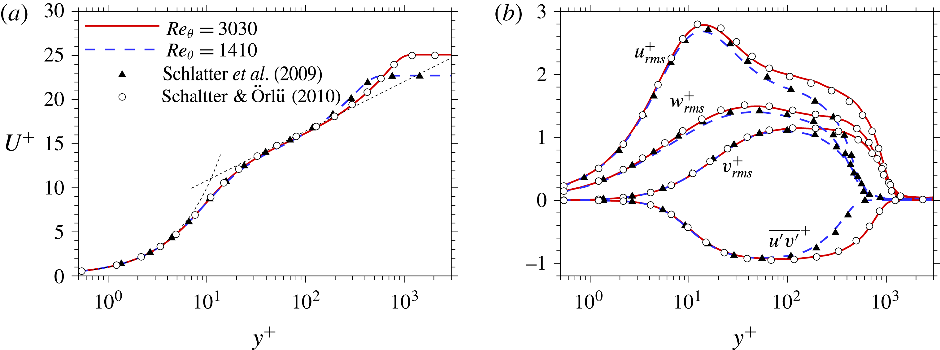
Profiles of (
 $a$
) mean streamwise velocity and (
 $b$
) turbulent stresses at
 $Re_{\unicode[STIX]{x1D703}}=1410$
and
 $3030$
. Note that the fluctuating components are evaluated relative to the conventional mean velocities.

The streamwise, wall-normal and spanwise directions are denoted
 $x$
,
 $y$
and
 $z$
, and the three components of velocity in those directions are
 $u$
,
 $v$
and
 $w$
. The computational domain was rectangular in shape, with periodic boundary conditions enforced in the span. The bottom wall was a no-slip surface, and a free-stress condition was enforced at the top of the domain as well as a suction velocity that maintained a zero streamwise mean pressure gradient. A convective outflow condition was applied at the exit plane.
Summary of simulation parameters.

The simulation was performed in two stages: a precursor simulation of laminar–turbulent transition and a main simulation for the fully turbulent regime; see table 1 for the parameters of both computations. The current dataset from the main simulation has similar or slightly finer resolution than the DNS by Kong, Choi & Lee (Reference Kong, Choi and Lee2000) of a TBL and by Min & Kim (Reference Min and Kim2004) of turbulent channel flow, which use a similar numerical scheme to the present work. The purpose of the precursor simulation was to generate realistic, time-dependent turbulent inflow data for the main computation. The Reynolds number based on the boundary-layer thickness at the inlet,
 $\unicode[STIX]{x1D6FF}_{0}$
, of the precursor simulation was
 $Re_{\unicode[STIX]{x1D6FF}}=800$
, which corresponds to
 $Re_{\unicode[STIX]{x1D703}}=108$
. Inflow perturbations with turbulence intensity less than 5 % were superimposed onto the Blasius profile in the region
 $0<y/\unicode[STIX]{x1D6FF}_{0}<2$
. Transition took place downstream via a bypass mechanism and the time-dependent flow field was stored in a cross-flow plane at
 $Re_{\unicode[STIX]{x1D703}}=1200$
, which is sufficiently upstream of the exit plane. The time-dependent plane data provided the inlet condition for the main computation at
 $Re_{\unicode[STIX]{x1D703}}=1200$
. Other boundary conditions were unchanged. The friction Reynolds number varies from
 $Re_{\unicode[STIX]{x1D70F}}=445$
to
 $1122$
. The
 $Re$
range is moderate in comparison with other DNS studies in recent literature. Nonetheless, the main results are evaluated at
 $Re_{\unicode[STIX]{x1D70F}}=1000$
, which is regarded as a fully turbulent state according to Schlatter & Örlü (Reference Schlatter and Örlü2012). Figure 1 shows the wall-normal profiles of the mean streamwise velocity and turbulent stresses, and demonstrates good agreement with previous results (Schlatter et al.
Reference Schlatter, Örlü, Li, Brethouwer, Fransson, Johansson, Alfredsson and Henningson2009; Schlatter & Örlü Reference Schlatter and Örlü2010). For the present study, a total of
 $1200$
instantaneous flow fields were stored in the region
 $300\leqslant x/\unicode[STIX]{x1D703}_{in}\leqslant 1050$
, where
 $x$
is measured from the inlet plane. This range corresponds to
 $1840\leqslant Re_{\unicode[STIX]{x1D703}}\leqslant 3190$
. The time interval between consecutive snapshots was
 $\unicode[STIX]{x0394}t=2\unicode[STIX]{x1D703}_{in}/U_{\infty }$
. Throughout the present work, overbar
 $\overline{\cdot }$
and angled brackets
 $\langle \cdot \rangle$
represent the unconditional and conditional statistics, respectively.
2.2 Structure identification
2.2.1 Turbulent/non-turbulent interface
The vorticity magnitude,
 $|\unicode[STIX]{x1D714}|\equiv (\unicode[STIX]{x1D714}_{i}\unicode[STIX]{x1D714}_{i})^{1/2}$
, was used as a detector function to identify the T/NT interface which demarcates rotational and irrotational regions of the flow (Jiménez et al.
Reference Jiménez, Hoyas, Simens and Mizuno2010; da Silva et al.
Reference da Silva, Hunt, Eames and Westerweel2014; Borrell & Jiménez Reference Borrell and Jiménez2016; Jahanbakhshi & Madnia Reference Jahanbakhshi and Madnia2016). The normalized vorticity magnitude is defined as
 $|\unicode[STIX]{x1D714}|^{\ast }\equiv |\unicode[STIX]{x1D714}|\sqrt{\unicode[STIX]{x1D6FF}^{+}}(\unicode[STIX]{x1D708}/u_{\unicode[STIX]{x1D70F}}^{2})$
, where
 $\unicode[STIX]{x1D6FF}$
and
 $u_{\unicode[STIX]{x1D70F}}$
are the local boundary-layer thickness and the friction velocity (Borrell & Jiménez Reference Borrell and Jiménez2016). The normalization is intended to provide a
 $Re$
-independent threshold, which was verified for the Reynolds number range considered here (see also appendix A for how this threshold relates to the vortical fluid fraction criterion). Due to the lack of a consensus on the
 $|\unicode[STIX]{x1D714}|^{\ast }$
threshold level, various studies have selected different thresholds,
 $|\unicode[STIX]{x1D714}|_{th}^{\ast }$
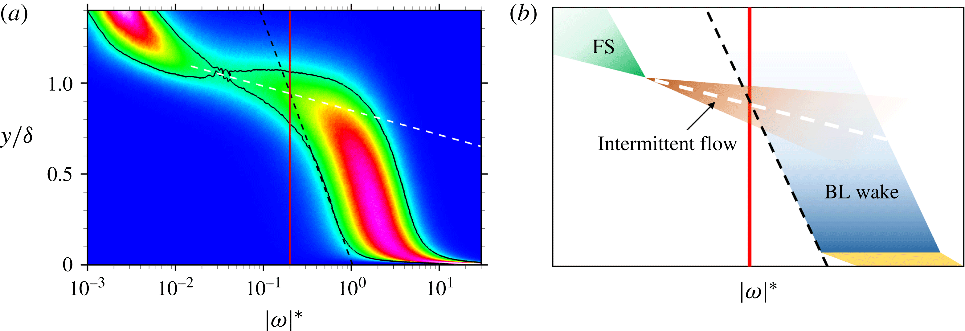
. We herein summarize our procedure for selecting its value. The starting point is the probability density function (p.d.f.) of
 $\log _{10}|\unicode[STIX]{x1D714}|^{\ast }$
at different heights from the wall (see figure 2). Two dashed lines are marked on the figure: the black dashed line marks the slope of the lowest p.d.f. contour, which captures the decay of vorticity in the outer boundary-layer flow. The white dashed line traces the ridge in the p.d.f., or the geometric centre of the contour, in the outer intermittent flow regime. The intersection of these two lines was selected as the vorticity threshold,
 $|\unicode[STIX]{x1D714}|_{th}^{\ast }=0.2$
, regardless of
 $Re$
. With this choice the average interface height is approximately
 $\unicode[STIX]{x1D6FF}$
.
(
 $a$
) Probability density function (p.d.f.) of
 $\log _{10}|\unicode[STIX]{x1D714}|^{\ast }$
at
 $Re_{\unicode[STIX]{x1D70F}}=1000$
: (red vertical)
 $|\unicode[STIX]{x1D714}|^{\ast }=0.2$
; (black) p.d.f.
 $=$
0.41; (black dashed) boundary-layer wake regime; (white dashed) intermittent flow regime. (
 $b$
) Schematic of the flow regimes. The symbols ‘FS’ and ‘BL’ denote the free stream and the boundary layer.

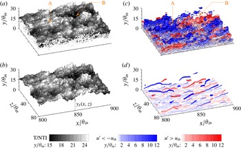
A sample result of the T/NT interface identification in an instantaneous flow field is shown in figure 3(
 $a$
). Originally, folds in the interface (or ‘pocket’ in the terminology by Borrell & Jiménez (Reference Borrell and Jiménez2016)) and irrotational blobs inside the turbulent region (or ‘bubble’) cause multiplicity of the interface height at a given (
 $x$
,
 $z$
) position. In the present work, focus is placed on the effect of LSM on the outer interface, and these folds in the surface were eliminated (see figure 3
 $b$
) by taking the interface envelope, similar to the approach by Bisset et al. (Reference Bisset, Hunt and Rogers2002). Irrotational regions surrounded by turbulent fluid and turbulent regions surrounded by irrotational fluid are excluded from the envelope. The height of the interface, measured relative to the bottom wall, is denoted
 $y_{I}$
.
Isosurfaces of (
 $a$
) the T/NT interface (
 $|\unicode[STIX]{x1D714}|_{th}^{\ast }=0.2$
) and (
 $b$
) interface envelope. (
 $c$
) Original fluctuating velocity field with
 $u^{\prime }=-0.1U_{\infty }$
(blue) and
 $0.1U_{\infty }$
(red). (
 $d$
) Detected cores for low- (blue) and high-speed (red) LSMs. Isosurfaces are coloured by wall-normal distance.

2.2.2 Large-scale motion
Large-scale coherence of the streamwise velocity fluctuations is a typical characteristic in wall-bounded turbulent flows (Adrian et al.
Reference Adrian, Meinhart and Tomkins2000). Figure 3(
 $c$
) shows an example of this large-scale coherence, identified by isosurface of
 $u_{th}^{\prime }=0.1U_{\infty }$
, which is the same threshold adopted by Dennis & Nickels (Reference Dennis and Nickels2011). Note that the fluctuating velocities
 $u_{i}^{\prime }$
are defined relative to the conditional turbulent,
 $\langle u_{i}\rangle _{T}$
, and non-turbulent,
 $\langle u_{i}\rangle _{NT}$
, mean values,
 $$\begin{eqnarray}u_{i}^{\prime }=\left\{\begin{array}{@{}ll@{}}u_{i}-\langle u_{i}\rangle _{T} & \text{if }|\unicode[STIX]{x1D714}|^{\ast }\geqslant |\unicode[STIX]{x1D714}|_{th}^{\ast }\text{(turbulent)},\\ u_{i}-\langle u_{i}\rangle _{NT} & \text{if }|\unicode[STIX]{x1D714}|^{\ast }<|\unicode[STIX]{x1D714}|_{th}^{\ast }\text{(non-turbulent)},\\ \end{array}\right.\end{eqnarray}$$
because only the conditional mean is a suitable reference in the intermittent region (Bisset et al.
Reference Bisset, Hunt and Rogers2002). Use of a conventional mean, e.g. unconditional time average, leads to artificial fluctuations in the non-turbulent free stream, which are effectively avoided by the present approach. The conditional mean in (2.1) is only a function of the streamwise and wall-normal locations,
 $\langle u_{i}\rangle _{T,NT}(x,y)$
. The mean can additionally be defined as a function of the distance of the interface,
 $\langle u_{i}\rangle (x,y,y_{I})$
, as proposed by Kwon et al. (Reference Kwon, Hutchins and Monty2016). Their approach is similarly effective in removing the free-stream artificial perturbations, but its statistical convergence is more difficult to achieve which led Kwon et al. (Reference Kwon, Hutchins and Monty2016) to apply local streamwise averaging despite the spatial inhomogeneity of the flow.
As demonstrated by figure 3(
 $c$
), the shape of the LSM in the instantaneous flow field is complex, and obfuscated by the small-scale features of turbulence. The LSMs can, however, be identified and tracked using the technique developed by Nolan & Zaki (Reference Nolan and Zaki2013) for transitional flows, and later extended for fully turbulent flows (Lee et al.
Reference Lee, Lee, Choi and Sung2014; Hwang et al.
Reference Hwang, Lee, Sung and Zaki2016). The algorithm consists of two steps. First, a Gaussian filter is adopted in the cross-flow plane to eliminate of the small-scale turbulence. The filtered velocity fluctuation
 $\hat{u}$
is defined as
 $$\begin{eqnarray}\hat{u} (x,y,z)=\mathop{\sum }_{z_{p}}\mathop{\sum }_{y_{p}}u_{i}^{\prime }(x,y_{p},z_{p})\underbrace{C(x,y,z)\exp \left(-\left(\frac{(y_{p}-y)^{2}}{2\unicode[STIX]{x1D70E}^{2}}+\frac{(z_{p}-z)^{2}}{2\unicode[STIX]{x1D70E}^{2}}\right)\right)\unicode[STIX]{x0394}y\unicode[STIX]{x0394}z}_{K(y_{p},z_{p};x,y,z)},\end{eqnarray}$$
where
 $y_{p}$
and
 $z_{p}$
are the grid locations within the window, centred at
 $(y,z)$
. The coefficients
 $C$
ensure that the summation of the Gaussian kernel,
 $K$
, is unity,
 $$\begin{eqnarray}\mathop{\sum }_{z_{p}}\mathop{\sum }_{y_{p}}K(y_{p},z_{p};x,y,z)=1.\end{eqnarray}$$
The standard deviation
 $\unicode[STIX]{x1D70E}(x,y)$
was determined from the spanwise width of the auto-correlation of
 $u^{\prime }$
, specifically
 $R_{u^{\prime }u^{\prime }}(\unicode[STIX]{x0394}z)=0.5$
, at every
 $(x,y)$
position. Earlier studies of streamwise periodic flows adopted a low-pass filter in that direction (Lee et al.
Reference Lee, Lee, Choi and Sung2014; Hwang et al.
Reference Hwang, Lee, Sung and Zaki2016), but the lack of homogeneity in the streamwise direction obviates this possibility. For this reason, we adopt the Gaussian filter in both the cross-flow plane and the streamwise direction.
From the filtered perturbation field,
 $\hat{u}$
, we proceed to identify the cores of the structures using local extrema and their connectivity in the streamwise direction. The spatial coordinates of high- and low-speed structure,
 $s$
, are denoted
 $\boldsymbol{x}^{s+}$
and
 $\boldsymbol{x}^{s-}$
, where
 $$\begin{eqnarray}\displaystyle \boldsymbol{x}^{s+}=\boldsymbol{x}\quad & \text{if }\unicode[STIX]{x2202}\hat{u} /\unicode[STIX]{x2202}z=\unicode[STIX]{x2202}\hat{u} /\unicode[STIX]{x2202}y=0\text{ and} & \displaystyle \hat{u} >\hat{u} _{th},\end{eqnarray}$$
 $$\begin{eqnarray}\displaystyle \boldsymbol{x}^{s-}=\boldsymbol{x}\quad & \text{if }\unicode[STIX]{x2202}\hat{u} /\unicode[STIX]{x2202}z=\unicode[STIX]{x2202}\hat{u} /\unicode[STIX]{x2202}y=0\text{ and} & \displaystyle \hat{u} <-\hat{u} _{th}.\end{eqnarray}$$
The threshold in the filtered field,
 $\hat{u} _{th}\equiv u_{th}^{\prime }(\langle u^{\prime }\hat{u} \rangle /\langle u^{\prime }u^{\prime }\rangle )$
, is equivalent to
 $u_{th}^{\prime }=0.1U_{\infty }$
in the original perturbation velocity. Connectivity of these local extrema has the appearance of elongated spines, which are the cores of the LSMs for low- (blue) and high- (red) speed structures (figure 3
 $d$
). In contrast to the raw turbulence field (figure 3
 $c$
), the detected cores clearly identify the characteristic position of the LSMs. By cross-correlating structures in consecutive flow fields, they can be tracked in time as Lagrangian objects (see movie 1, available at https://doi.org/10.1017/jfm.2017.170).
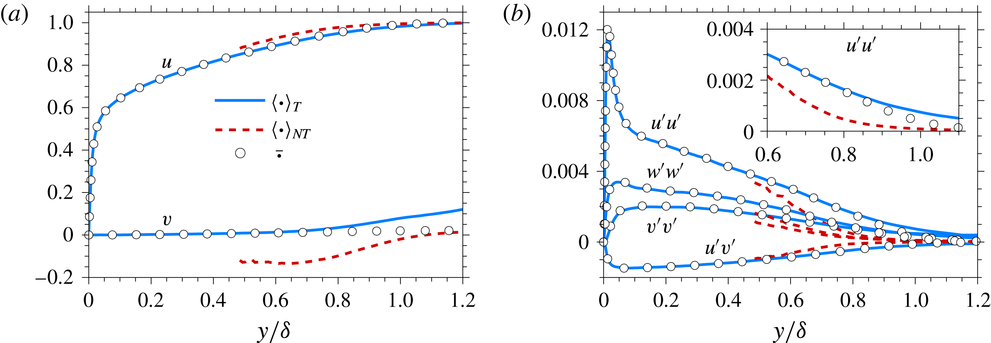
Profiles of conditionally averaged statistics by
 $|\unicode[STIX]{x1D714}|_{th}^{\ast }=0.2$
at
 $Re_{\unicode[STIX]{x1D70F}}=1000$
. (
 $a$
) Mean velocity and (
 $b$
) turbulent stresses. The number of samples is larger than
 $1\,\%$
of the total number of data at each
 $y$
-position.

3 Results
First, we evaluate conditionally sampled statistics based on the T/NT discrimination. Beyond the direct interest in these statistics, the conditional mean is also used to evaluate the perturbation field. Figure 4(
 $a$
) shows the conditional mean velocity,
 $\langle u_{i}\rangle _{T}$
and
 $\langle u_{i}\rangle _{NT}$
, at
 $Re_{\unicode[STIX]{x1D70F}}=1000$
. Because turbulence is persistent close to the wall, the unconditional (or conventional) mean,
 $$\begin{eqnarray}\overline{u_{i}}\equiv \unicode[STIX]{x1D6FE}\langle u_{i}\rangle _{T}+(1-\unicode[STIX]{x1D6FE})\langle u_{i}\rangle _{NT},\end{eqnarray}$$
and the turbulent conditional average,
 $\langle u_{i}\rangle _{T}$
, are identical in that region. In (3.1),
 $\unicode[STIX]{x1D6FE}$
is the intermittency factor. Near the boundary-layer edge, however, the unconditional statistics differ from both the turbulent and the non-turbulent profiles. The deviation is more evident in the vertical velocity than in the streamwise velocity. Inside the boundary layer, the non-turbulent conditioned
 $v$
profile,
 $\langle v\rangle _{NT}$
, is negative which signifies the entrainment of outer, or free-stream, non-turbulent fluid into the boundary layer. Conversely, the turbulent conditioned
 $v$
profile,
 $\langle v\rangle _{T}$
, is positive outside the boundary layer since the observation of turbulence beyond
 $y=\unicode[STIX]{x1D6FF}$
is associated with ejections. It is also important to note that the present results depend on the choice of the vorticity threshold for the identification of the T/NT interface. A higher threshold would move the interface deeper into the boundary layer and exaggerate the difference between the conditional and conventional averages (appendix B).
The conditional average of the turbulent stress,
 $$\begin{eqnarray}\langle u_{i}^{\prime }u_{j}^{\prime }\rangle _{T}\equiv \langle \left(u_{i}-\langle u_{i}\rangle _{T}\right)\left(u_{j}-\langle u_{j}\rangle _{T}\right)\rangle _{T},\end{eqnarray}$$
is shown in figure 4(
 $b$
). The stress at the turbulent side is similar to or slightly larger than the conventional average (see the inset of figure 4(
 $b$
) for the streamwise stress, for example),
 $$\begin{eqnarray}\displaystyle \overline{u_{i}^{\prime }u_{j}^{\prime }} & \equiv & \displaystyle \unicode[STIX]{x1D6FE}\langle u_{i}^{\prime }u_{j}^{\prime }\rangle _{T}+(1-\unicode[STIX]{x1D6FE})\langle u_{i}^{\prime }u_{j}^{\prime }\rangle _{NT}\nonumber\\ \displaystyle & & \displaystyle +\,\unicode[STIX]{x1D6FE}(1-\unicode[STIX]{x1D6FE})\left(\langle u_{i}\rangle _{T}-\langle u_{i}\rangle _{NT}\right)\left(\langle u_{j}\rangle _{T}-\langle u_{j}\rangle _{NT}\right).\end{eqnarray}$$
The degree of intermittency determines the deviation of the conventional and conditional averages and, for the present choice of
 $|\unicode[STIX]{x1D714}|_{th}^{\ast }$
, it is not sufficiently large to cause an appreciable disparity.
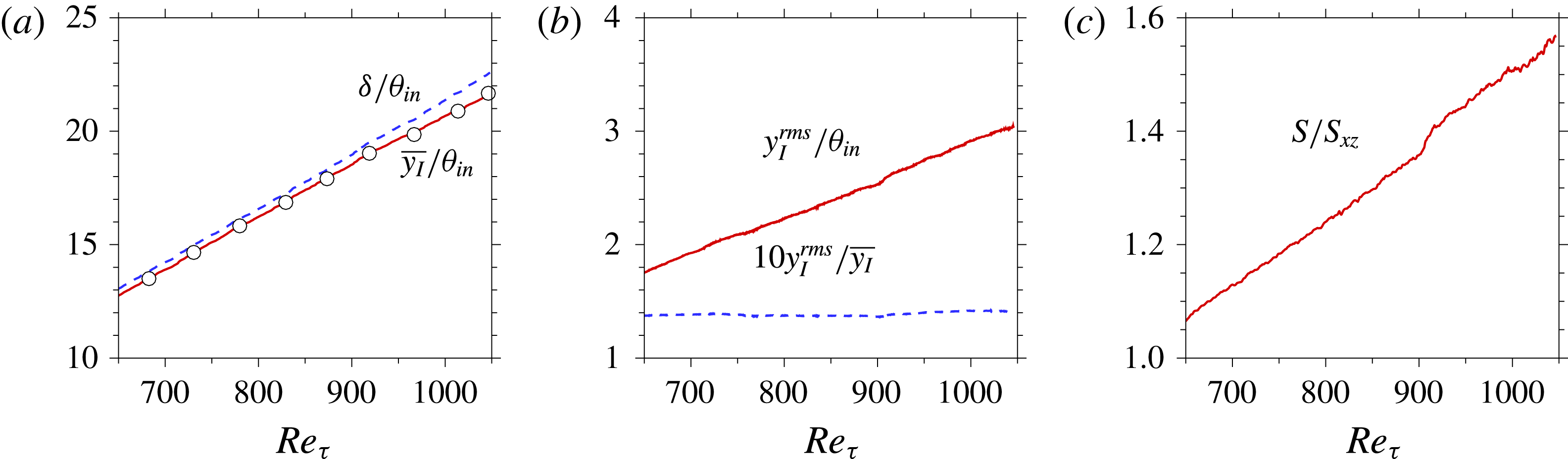
Streamwise distribution of (
 $a$
) mean height of the T/NT interface,
 $\overline{y_{I}}$
, (
 $b$
) the root-mean-square of the fluctuation,
 $y_{I}^{rms}$
and (
 $c$
) the interface area per unit projected area in the horizontal plane,
 $S/S_{xz}$
. (Circles) Intermittency factor
 $\unicode[STIX]{x1D6FE}=0.5$
.

3.1 Properties of the interface
The mean height of the T/NT interface,
 $\overline{y_{I}}$
, as a function of
 $Re_{\unicode[STIX]{x1D70F}}$
is shown in figure 5(
 $a$
). The boundary-layer thickness
 $\unicode[STIX]{x1D6FF}$
and the intermittency factor
 $\unicode[STIX]{x1D6FE}=0.5$
are also overlaid for comparison. The mean position of the interface (figure 5
 $a$
) coincides with the position of
 $\unicode[STIX]{x1D6FE}=0.5$
. On the other hand, the position of
 $\unicode[STIX]{x1D6FE}=0.425$
(not shown) is identical to the local 99 % boundary-layer thickness. The agreement between a constant
 $\unicode[STIX]{x1D6FE}$
and
 $\unicode[STIX]{x1D6FF}(x)$
is qualitatively similar to the results by Vinuesa et al. (Reference Vinuesa, Bobke, Örlü and Schlatter2016), although the
 $\unicode[STIX]{x1D6FE}$
value is not identical due to the difference in the detector function and threshold. In addition,
 $\overline{y_{I}}$
grows with
 $Re_{\unicode[STIX]{x1D70F}}$
at a slightly smaller rate than the boundary-layer thickness
 $\unicode[STIX]{x1D6FF}(x)$
. The boundary-layer thickness and the T/NT interface height are two flow thicknesses based on the mean streamwise momentum and the turbulence activity, respectively. Hence, the increasing gap between
 $\overline{y_{I}}$
and
 $\unicode[STIX]{x1D6FF}$
downstream suggests that the intermittency of the boundary-layer turbulence becomes more significant at higher Reynolds number, and as such, a larger region below the mean boundary-layer edge is encroached by sweeping free-stream laminar flow. The root-mean-square (r.m.s.) of the interface height fluctuation,
 $y_{I}^{rms}$
, is plotted in figure 5(
 $b$
). The excursions of the interface away from its mean location clearly increase in magnitude as the Reynolds number increases downstream. The increase is proportional to the growth of the interface height, or equivalently the boundary-layer thickness, and is most evident when
 $y_{I}^{rms}$
is normalized by the inlet momentum thickness. The more pronounced excursions of the interface at higher Reynolds numbers imply that larger regions of laminar free-stream fluid will encroach onto the TBL, and vice versa. Another outcome is an increase in the interfacial surface area (figure 5
 $c$
) and entrainment at higher Reynolds numbers, which is consistent with our understanding of high-
 $Re$
flows (de Silva et al.
Reference de Silva, Philip, Chauhan, Meneveau and Marusic2013; Chauhan et al.
Reference Chauhan, Philip, de Silva, Hutchins and Marusic2014b
), although the ratio is smaller than previous studies since we are only concerned with the LSM and envelope.
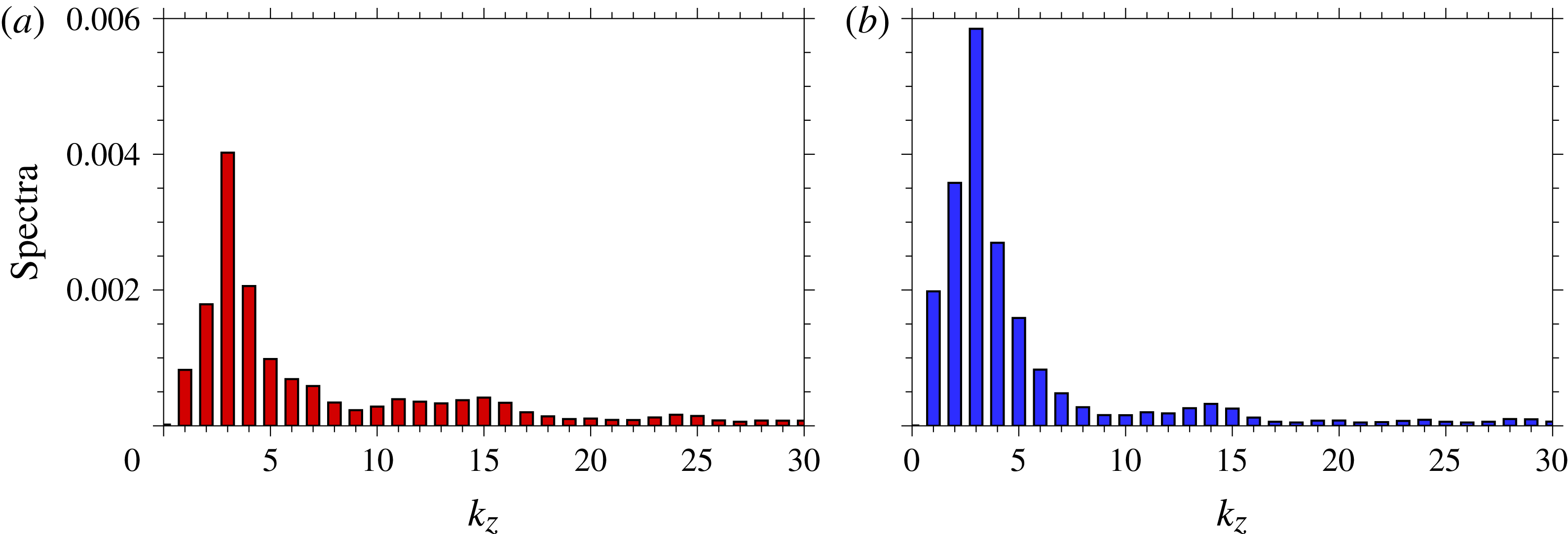
A spectral analysis of the interface height can effectively characterize its undulation. Figure 6 shows the spanwise spectra of the normalized fluctuation in the T/NT interface height,
 $$\begin{eqnarray}Y_{I}^{\prime }(x,z)=\frac{y_{I}(x,z)-\overline{y_{I}}(x)}{\overline{y_{I}}(x)}.\end{eqnarray}$$
Fourier coefficients of the spanwise spectra at both
 $Re_{\unicode[STIX]{x1D70F}}=680$
and
 $1000$
peak at spanwise wavenumber
 $k_{z}=3$
. As the Reynolds number increases, the Fourier coefficients of low-
 $k_{z}$
modes (
 $k_{z}\lesssim 10$
) become more pronounced, while higher wavenumbers of the normalized fluctuations (
 $k_{z}\gtrsim 10$
) become relatively less important. In other words, the large-scale deformation becomes dominant downstream. A significant aspect of the interface deformation in the span is thus of the order of the boundary-layer thickness. The spectra demonstrate the large-scale nature of the interface morphology and suggests a possible relationship between this morphology and the large-scale turbulent structures inside the boundary layer.
Spanwise spectra of the normalized interface height fluctuation
 $Y_{I}^{\prime }$
at (
 $a$
)
 $Re_{\unicode[STIX]{x1D70F}}=680$
and (
 $b$
)
 $Re_{\unicode[STIX]{x1D70F}}=1000$
.

Since the interface undulations intensify downstream with the growth of the boundary layer,
 $y_{i}^{\prime }\sim \unicode[STIX]{x1D6FF}(x)\sin (x)$
, spectra were not computed in that dimension. Instead, the two-point correlation,
 $$\begin{eqnarray}R_{Y_{I}^{\prime }Y_{I}^{\prime }}(r_{x},r_{z})=\frac{\langle Y_{I}^{\prime }(x_{ref},z)Y_{I}^{\prime }(x_{ref}+r_{x},z+r_{z})\rangle }{\unicode[STIX]{x1D70E}_{Y_{I}^{\prime }}(x_{ref})\unicode[STIX]{x1D70E}_{Y_{I}^{\prime }}(x_{ref}+r_{x})},\end{eqnarray}$$
was evaluated to examine the characteristics of the interface. In the above expression,
 $\unicode[STIX]{x1D70E}_{Y_{I}^{\prime }}$
is the standard deviation of the normalized fluctuation. For comparison, the auto-correlations of
 $u^{\prime }$
and
 $v^{\prime }$
at the wall-normal reference position
 $y_{ref}=\overline{y_{I}}$
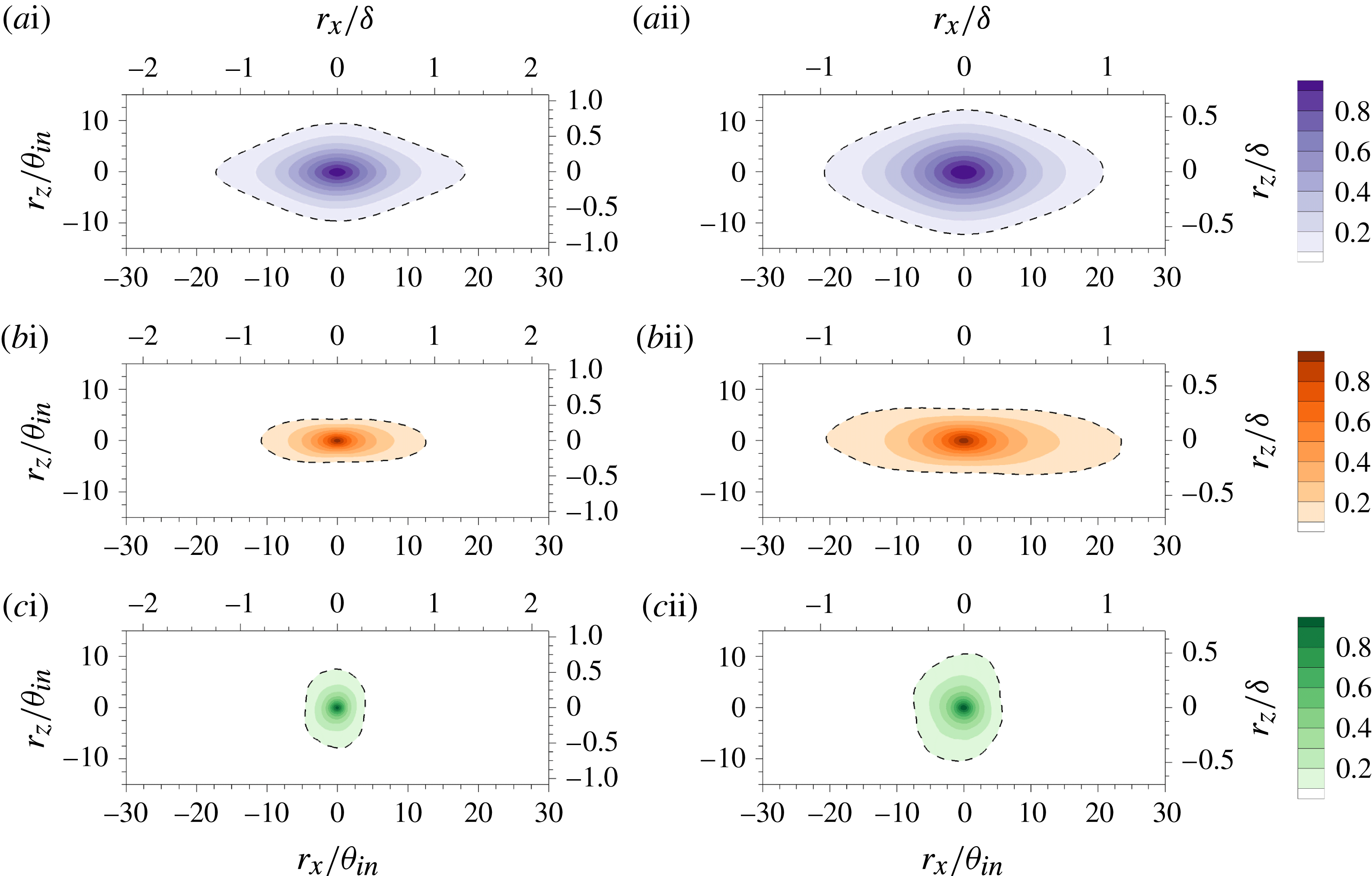
were also computed. The results are plotted in figure 7 at two downstream locations. The fluctuating interface height shows stronger correlation in the streamwise direction in comparison with the span. The shape of
 $R_{Y_{I}^{\prime }Y_{I}^{\prime }}$
(figure 7
 $a$
) resembles the two-point correlation of the streamwise velocity fluctuations
 $R_{u^{\prime }u^{\prime }}$
(figure 7
 $b$
), although the aspect ratio of
 $R_{Y_{I}^{\prime }Y_{I}^{\prime }}$
is smaller. Based on the contour of
 $R=0.1$
(dashed line), the streamwise extents of both
 $R_{Y_{I}^{\prime }Y_{I}^{\prime }}$
and
 $R_{u^{\prime }u^{\prime }}$
are approximately
 $2\unicode[STIX]{x1D6FF}$
, and their streamwise dimensions normalized by the reference length scale,
 $\unicode[STIX]{x1D703}_{in}$
, increase slightly with Reynolds number. The streamwise extent of the interface ridge (or groove), therefore, is as long as the large-scale turbulent motions. In contrast, the correlation of the wall-normal fluctuations
 $R_{v^{\prime }v^{\prime }}$
(figure 7
 $c$
) is shorter in streamwise extent, which is consistent with Ganapathisubramani et al. (Reference Ganapathisubramani, Hutchins, Hambleton, Longmire and Marusic2005) and Sillero, Jiménez & Moser (Reference Sillero, Jiménez and Moser2014). The shorter
 $v^{\prime }$
-coherence is dominated by the spanwise vortices in the intermittent region, which are clustered around large-scale
 $u^{\prime }$
-structures (Lozano-Durán, Flores & Jiménez Reference Lozano-Durán, Flores and Jiménez2012). The similarity between the streamwise size of the interface deformation and of the large-scale
 $u^{\prime }$
-coherence motivates study of the T/NT interface characteristics conditioned on the LSMs.
Two-point correlations in the wall-parallel plane. (
 $a$
) The interface height fluctuations
 $Y_{I}^{\prime }$
, (
 $b$
) the streamwise velocity fluctuations
 $u^{\prime }$
and (
 $c$
) the wall-normal velocity fluctuations
 $v^{\prime }$
. The reference streamwise positions are located at (i)
 $Re_{\unicode[STIX]{x1D70F}}=680$
and (ii)
 $Re_{\unicode[STIX]{x1D70F}}=1000$
. In (b,c), the reference wall-normal position is at
 $y=\overline{y_{I}}$
. The dashed contour marks
 $R=0.1$
.

3.2 Connection between interface deformation and LSM
The results in § 3.1 suggest a connection between the interface and the LSMs. Flow visualizations, such as in figure 3, which shows the LSMs and the deformed T/NT interface, also support the same view. For example, the interface is convex above the low-speed structure (marked ‘A’ in figure 3 a,b), and concave above high-speed structures (marked ‘B’). To clarify and generalize such observations, conditional sampling is used to evaluate the effects of the low- and the high-speed structures on the interface.
The wall-normal positions of the T/NT interface and of the core of the LSM are denoted
 $y_{I}$
and
 $y^{s\pm }$
, respectively. The latter can be further classified into the cores of low- and high-speed structures,
 $y^{s-}$
and
 $y^{s+}$
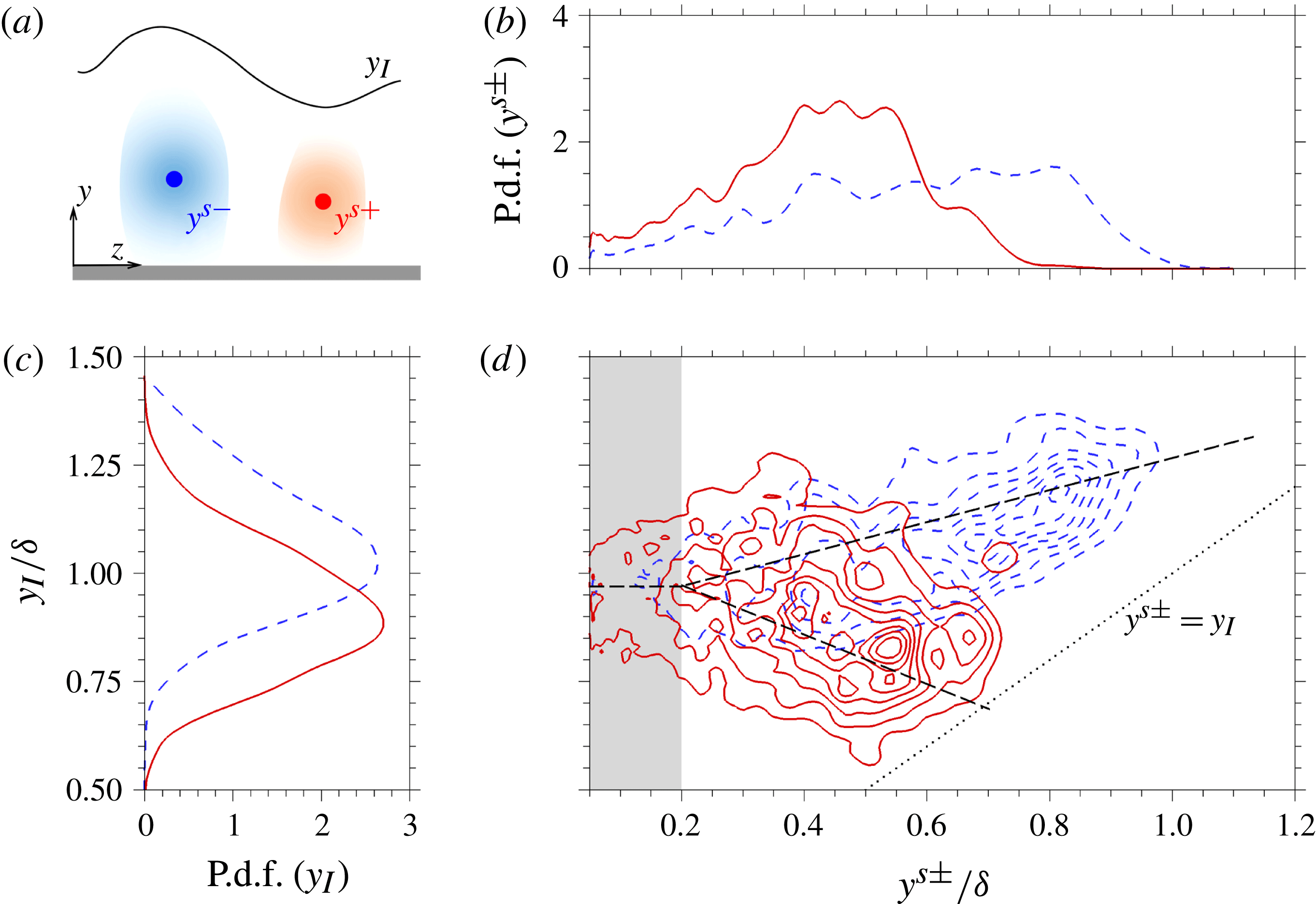
, according to (2.4) and (2.5). As shown schematically in figure 8(
 $a$
), the core represents a certain position within the structure in the cross-flow plane, while the full structure occupies a large wall-normal and spanwise area around that position. In order to evaluate the correlation between
 $y_{I}$
and
 $y^{s\pm }$
, the p.d.f. of each quantity alone (figure 8
b,c) and the joint p.d.f. are computed and visualized in figure 8(
 $d$
).
(
 $a$
) Schematic of the LSM and the detected core in the cross-flow plane. Probability density functions of the interface height
 $y_{I}$
and the vertical position of the detected cores
 $y^{s\pm }$
at
 $Re_{\unicode[STIX]{x1D70F}}=1000$
: (
 $b$
) p.d.f. of
 $y^{s\pm }$
; (
 $c$
) p.d.f. of
 $y_{I}$
; (
 $d$
) joint p.d.f. of
 $y^{s\pm }$
and
 $y_{I}$
. (Dashed) The low-speed LSM core
 $y^{s-}$
and (solid) the high-speed LSM core
 $y^{s+}$
. Bin sizes are
 $0.025\unicode[STIX]{x1D6FF}$
in
 $y_{I}$
and
 $\unicode[STIX]{x0394}y$
in local
 $y^{s\pm }$
.

The p.d.f. of
 $y^{s+}$
(figure 8
 $b$
, solid line) is finite in the range
 $y^{s+}\lesssim 0.8\unicode[STIX]{x1D6FF}$
only. The decay of the p.d.f. towards the edge of the boundary layer is symptomatic of the relatively small population of the high-speed LSMs away from the wall (Lee et al.
Reference Lee, Ahn and Sung2015). In contrast, the cores of the low-speed motions are more frequently observed near the boundary-layer edge, and thus their p.d.f. is finite throughout the range
 $y^{s-}\lesssim \unicode[STIX]{x1D6FF}$
(dashed line). In a previous study, Lozano-Durán et al. (Reference Lozano-Durán, Flores and Jiménez2012) evaluated the average perturbation fields conditional on the LSM. Their observation that sweeps are located away from the wall relative to ejections is consistent with the p.d.f. of
 $y^{s\pm }$
in the current study. Figure 8(
 $c$
) reports the p.d.f. of
 $y_{I}$
, conditioned on a finite value of
 $y^{s\pm }$
, or equivalently on the presence of a large-scale structure. The maximum probabilities of
 $y_{I}$
are recorded at
 $1.03\unicode[STIX]{x1D6FF}$
and
 $0.893\unicode[STIX]{x1D6FF}$
for the low- and high-speed structures, respectively. These values should be contrasted to the mean
 $\overline{y_{I}}=0.966\unicode[STIX]{x1D6FF}$
at the same streamwise position (see figure 5
 $a$
).
The joint p.d.f. of
 $y_{I}$
and
 $y^{s\pm }$
(figure 8
 $d$
) shows modulation of the interface height by the LSMs. When the detected core is located in the log region or more generally below
 $y^{s\pm }=0.2\unicode[STIX]{x1D6FF}$
(grey region in the figure), the median of the p.d.f. of the interface height is approximately equal to
 $\overline{y_{I}}$
for both low- and high-speed motions. In other words, there is no clear difference in the height of the T/NT interface when the underlying high- and low-speed structures are in the log region. However, the detected cores in the wake region (
 $y^{s\pm }>0.2\unicode[STIX]{x1D6FF}$
) have a noticeable impact on the interface, which is captured by the bifurcating dashed line in figure 8(
 $d$
). The interface height decreases, when the high-speed fluid is detected in the wake region, and increases in presence of low-speed structures. As a result, the vertical spacing between the interface and the cores of these large-scale structures is smaller for the high-speed ones than those at low speed. The difference is clear when contrasting the gap between the dotted line,
 $y^{s\pm }=y_{I}$
, and the two sets of contours in figure 8(
 $d$
). This result confirms that the wall-normal elevation of the T/NT interface is modulated by the underlying low- and high-speed LSMs in the wake region.
Conditional average of the normalized interface fluctuation based on the core of (
 $a$
) low- and (
 $b$
) high-speed LSMs. Reference position is located at
 $Re_{\unicode[STIX]{x1D70F}}=1000$
(
 $x_{ref}=963\unicode[STIX]{x1D703}_{in}$
) and
 $y_{ref}=0.5\unicode[STIX]{x1D6FF}$
, marked as a vertical line.

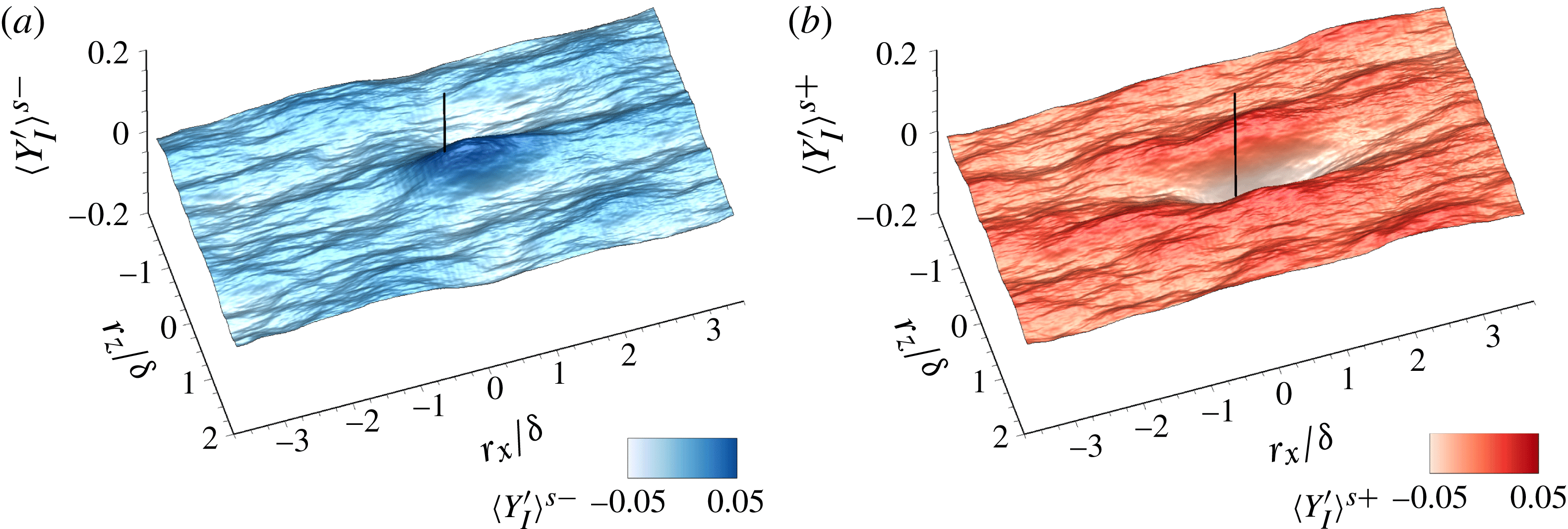
A statistical representation of the interface shape in the vicinity of positive and negative LSMs can be obtained by computing the conditional average,
 $$\begin{eqnarray}\langle y_{I}\rangle ^{s\pm }(r_{x},r_{z})=\langle y_{I}(x_{ref}+r_{x},z+r_{z})|x^{s\pm }=x_{ref},y^{s\pm }=y_{ref}\rangle .\end{eqnarray}$$
Figure 9 shows the isosurface of the result normalized by the mean interface height,
 $\langle Y_{I}^{\prime }\rangle ^{s\pm }\equiv (\langle y_{I}\rangle ^{s\pm }-\overline{y_{I}})/\overline{y_{I}}$
. The reference position is located at
 $x_{ref}=963\unicode[STIX]{x1D703}_{in}$
(or
 $Re_{\unicode[STIX]{x1D70F}}=1000$
) and
 $y_{ref}=0.5\unicode[STIX]{x1D6FF}$
. This wall-normal location is within the wake region, and therefore the probabilities of observing low- and high-speed streaks differ (figure 8
 $d$
). Above the low-speed structure (figure 9
 $a$
), the interface is displaced outward towards the free stream. Conversely, a depression in the interface height is observed above the high-speed structure at the reference position (figure 9
 $b$
). The streamwise dimension of the conditionally averaged interface elevation is approximately
 $2\unicode[STIX]{x1D6FF}$
which is consistent with that of
 $R_{Y_{I}^{\prime }Y_{I}^{\prime }}$
(figure 7
 $a$
ii) and
 $R_{u^{\prime }u^{\prime }}$
(figure 7
 $b$
ii). The displacements are not symmetric: the height of the crest above the low-speed structure is smaller than the depth of the trough associated with the high-speed motion. The figure also shows that the conditional interface shape is elongated in the streamwise direction and is narrow in the span. Similar to the two-point correlation
 $R_{Y_{I}^{\prime }Y_{I}^{\prime }}$
(figure 7
 $a$
ii), the spanwise dimension of the interface deformation, which is identified based on the location where
 $\langle Y_{I}^{\prime }\rangle ^{s\pm }=0$
, is approximately
 $1\unicode[STIX]{x1D6FF}$
. Beyond that width, an anti-correlated pattern is observed. Since the low-speed structure is flanked by high-speed structures and vice versa (e.g. Chung & McKeon Reference Chung and McKeon2010; Hwang et al.
Reference Hwang, Lee, Sung and Zaki2016), the alternating appearance of crests and troughs in the span is consistent with the arrangement and proposed influence of LSMs.
Conditionally averaged velocity fields based on the core of (i) low- and (ii) high-speed LSMs at
 $Re_{\unicode[STIX]{x1D70F}}=1000$
(
 $x_{ref}=963\unicode[STIX]{x1D703}_{in}$
) and
 $y_{ref}=0.5\unicode[STIX]{x1D6FF}$
. The figure is visualized in (
 $a$
) the cross-flow plane at
 $r_{x}=0$
and (
 $b$
) the side view at
 $r_{z}=0$
. Flood contour and velocity vectors are
 $\langle u^{\prime }\rangle ^{s\pm }$
and the in-plane velocity fluctuation vectors, respectively. (Solid) the position of the averaged T/NT interface; (dashed)
 $\langle u^{\prime }\rangle ^{s\pm }=\pm 0.02U_{\infty }$
.

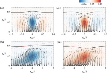
The local change of the T/NT interface height due to the underlying low- and high-speed motions is also examined by computing the conditional average,
 $$\begin{eqnarray}\langle u_{i}^{\prime }\rangle ^{s\pm }(r_{x},y,r_{z})=\langle u_{i}^{\prime }(x_{ref}+r_{x},y,z+r_{z})|x^{s\pm }=x_{ref},y^{s\pm }=y_{ref}\rangle .\end{eqnarray}$$
The reference position was again placed at
 $x_{ref}=963\unicode[STIX]{x1D703}_{in}$
(or
 $Re_{\unicode[STIX]{x1D70F}}=1000$
) and
 $y_{ref}=0.5\unicode[STIX]{x1D6FF}$
, and the results are shown in figure 10. The dashed line in the figure marks
 $\langle u^{\prime }\rangle ^{s\pm }=\pm 0.02U_{\infty }$
, and demonstrates that the shape of the LSM is comparable for both positive and negative velocity perturbations. The conditionally averaged velocity vectors confirm that the ejection event,
 $\langle u^{\prime }\rangle ^{s-}<0$
, is capped by a crest in the interface (figure 10
 $a$
i). In contrast, a sweep event,
 $\langle u^{\prime }\rangle ^{s+}>0$
, is clearly accompanied by a trough in the interface shape (figure 10
 $a$
ii). The subsidence of the interface is accompanied with the negative
 $\langle v^{\prime }\rangle ^{s+}$
. Also, although sweep events contribute favourably to the Reynolds shear stress and turbulence production, the associated T/NT interface is displaced towards the wall. As a result, the perturbation field associated with high-speed motion does not contribute to turbulence activity near the mean location of the boundary-layer edge.
In the side view (figure 10
 $b$
), the pitch angles of the interface and of the LSM are visible. The estimated angles of the latter (dash-dot line) are approximately
 $14^{\circ }$
for both the low- and high-speed structures. On the other hand, the inclination angle of the T/NT interface differs in the two configurations. Above the low-speed structures, the angle is positive and shallower, measuring
 $5.3^{\circ }$
(red solid line), which is in line with our understanding of wall-detached structures nearer to the edge of the boundary layer. Above the high-speed structure, the interface angle is negative, and is equal to
 $-4.9^{\circ }$
at the upstream position
 $-\unicode[STIX]{x1D6FF}\lesssim r_{x}\lesssim 0$
(figure 10
 $b$
ii).
Earlier work by Eisma et al. (Reference Eisma, Westerweel, Ooms and Elsinga2015), which did not differentiate the effect of low- and high-speed motion, showed a similarity in the turbulence statistics at the interface and at internal shear layers. In the present context, these layers correspond to the outer edges of the LSMs (Adrian et al. Reference Adrian, Meinhart and Tomkins2000; Christensen & Adrian Reference Christensen and Adrian2001; Adrian Reference Adrian2007). However, the conditionally sampled fields in figure 10 demonstrate the qualitative difference between the T/NT interface and the outer edge of the LSM, in particular for high-speed structures. This point is further emphasized by computing conditional statistics of the turbulence in the vicinity of the interface.
3.3 Conditional statistics in the vicinity of the interface
Previous studies have reported the turbulence statistics as a function of distance to the interface (e.g. Bisset et al. Reference Bisset, Hunt and Rogers2002; Chauhan et al. Reference Chauhan, Philip and Marusic2014a ; da Silva et al. Reference da Silva, Hunt, Eames and Westerweel2014). Since the low- and high-speed motions contribute differently to the conditional statistics in the bulk (Lee et al. Reference Lee, Ahn and Sung2015), it is anticipated that the near-interface statistics are also dependent on the adjacent LSMs. We therefore examine the low- and high-speed large scales, and evaluate their respective contributions to the near-interface dynamics.
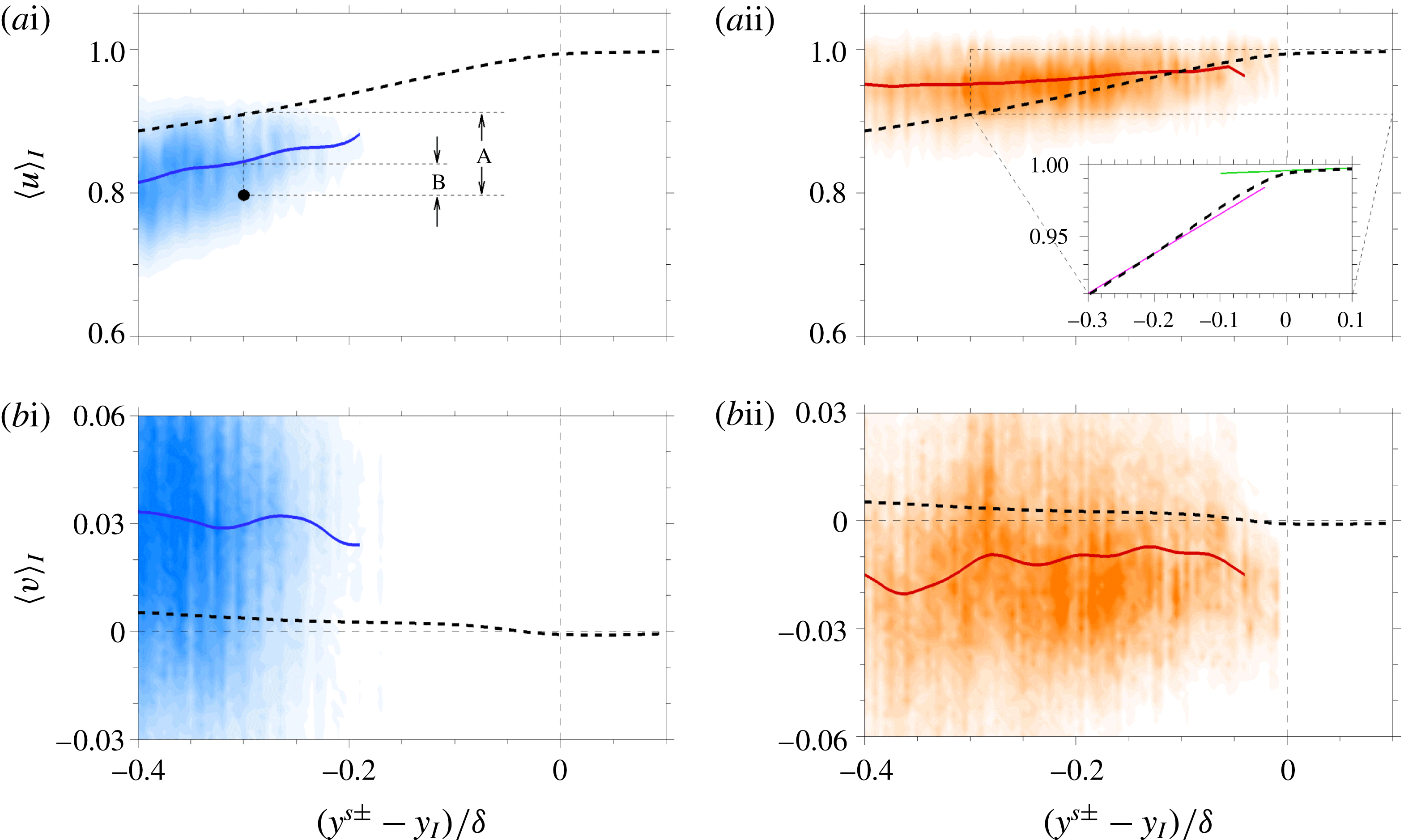
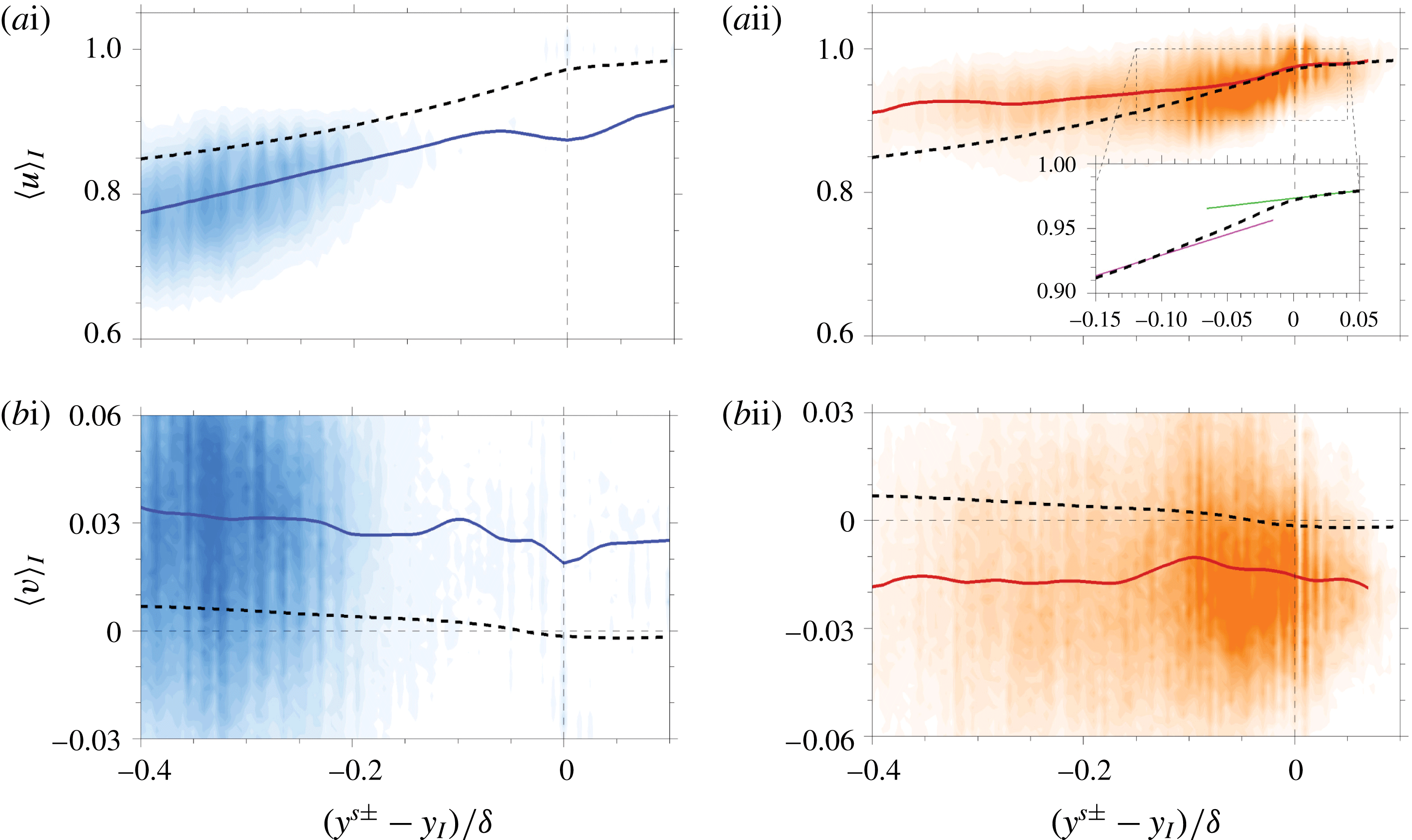
Joint p.d.f. of the conditional total velocity and the vertical distance of the LSM core from the interface (flood) at
 $Re_{\unicode[STIX]{x1D70F}}=1000$
. (Solid) The expected value of the p.d.f. of the conditional velocity at the LSM core. (
 $a$
) Streamwise and (
 $b$
) wall-normal velocities. (i) Low- and (ii) high-speed structures. The number of samples is larger than
 $1000$
at each
 $y$
-position. Dashed line indicates
 $\langle u_{i}\rangle _{I}$
.

Figure 11 shows the joint p.d.f. of the conditional total velocity and the vertical separation between the LSM core and the interface. The expected value of the probability distribution is also plotted. Similar to Ishihara et al. (Reference Ishihara, Ogasawara and Hunt2015), a local averaging in the streamwise direction is applied to improve convergence of the conditional mean,
 $$\begin{eqnarray}\langle u_{i}\rangle _{I}^{s\pm }(y^{s\pm }-y_{I})=\frac{1}{2\unicode[STIX]{x0394}L_{x}}\int _{x-\unicode[STIX]{x0394}L_{x}}^{x+\unicode[STIX]{x0394}L_{x}}\langle u_{i}(x,y-y_{I},z)|\boldsymbol{x}=\boldsymbol{x}^{s\pm }\rangle \,\text{d}x,\end{eqnarray}$$
where
 $\unicode[STIX]{x0394}L_{x}$
is set to
 $10\unicode[STIX]{x1D703}_{in}$
. Note that the average also includes points across the cores of the large-scale structures in the homogeneous spanwise direction. In addition to the conditional sampling based on the low- and high-speed structures separately, the mean velocity evaluated as a function of the vertical distance from the interface,
 $\langle u_{i}\rangle _{I}(y-y_{I})$
, is plotted for comparison (dotted line). The p.d.f. of the low-speed events (figure 11
 $a$
i) vanishes near the interface (
 $y^{s\pm }-y_{I}=0$
), while that of high-speed ones (figure 11
 $a$
ii) is finite. As such the expectation of observing a low-speed event, here defined with the core of LSM, is zero in the near-interface region, even though the structures are associated with ejections and their large volume can reach farther away from the wall than the high-speed counterparts. The p.d.f. of the positive LSM more closely shadows the unconditional mean profile near the T/NT interface.
Previous studies reported the presence of a rapid change in the mean streamwise velocity near the interface (e.g. Chauhan et al.
Reference Chauhan, Philip, de Silva, Hutchins and Marusic2014b
; Ishihara et al.
Reference Ishihara, Ogasawara and Hunt2015). As noted in the discussion of figure 4, such abrupt change is weak, e.g. in the inset of figure 11(
 $a$
ii), due to the small vorticity threshold
 $|\unicode[STIX]{x1D714}|^{\ast }$
adopted for the identification of the T/NT interface. The p.d.f. indicates that the jump in
 $\langle u\rangle _{I}$
coincides with the absence of low-speed events near the interface. High-speed events, on the other hand, do not contribute appreciably to the jump due to the weak shear near the outer edge of the boundary layer.
The p.d.f.s of the conditional vertical velocity are plotted in figure 11(
 $b$
). Consistent with the kinematics of ejections and sweeps (Wallace Reference Wallace2016), the low-speed LSM is mainly associated with positive
 $\langle v\rangle _{I}$
and the high-speed LSMs are due to negative
 $\langle v\rangle _{I}$
. The distinction here is that the origin of the vertical coordinate axis is attached to the interface, and we report the advection velocity of the boundary-layer, or vortical, flow only. In addition, the figure also shows the entraining motion beneath the interface, where the high-speed event is predominant.
Previous studies examined the sudden change in the turbulence stresses near the interface (Chauhan et al.
Reference Chauhan, Philip, de Silva, Hutchins and Marusic2014b
; Eisma et al.
Reference Eisma, Westerweel, Ooms and Elsinga2015; Ishihara et al.
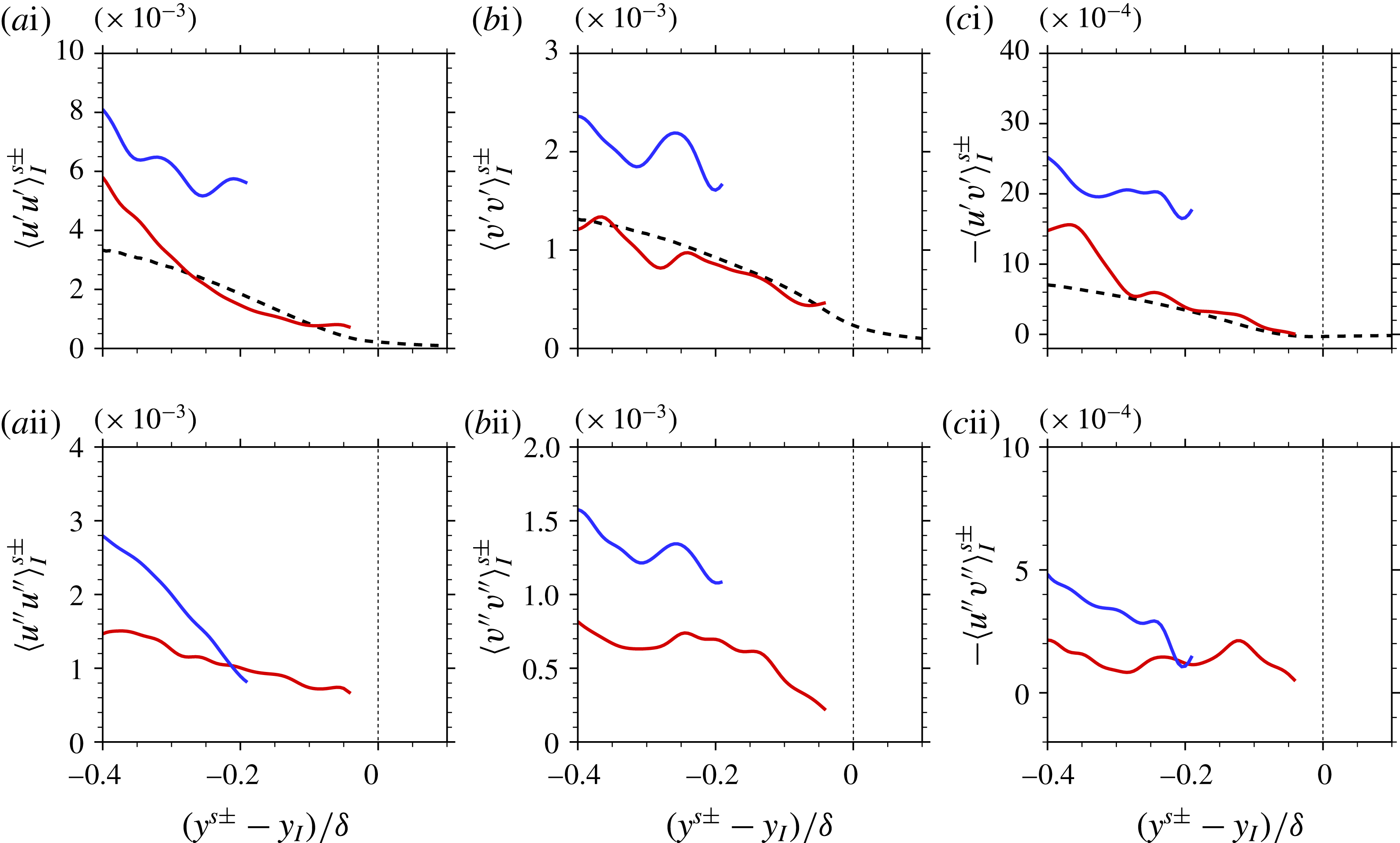
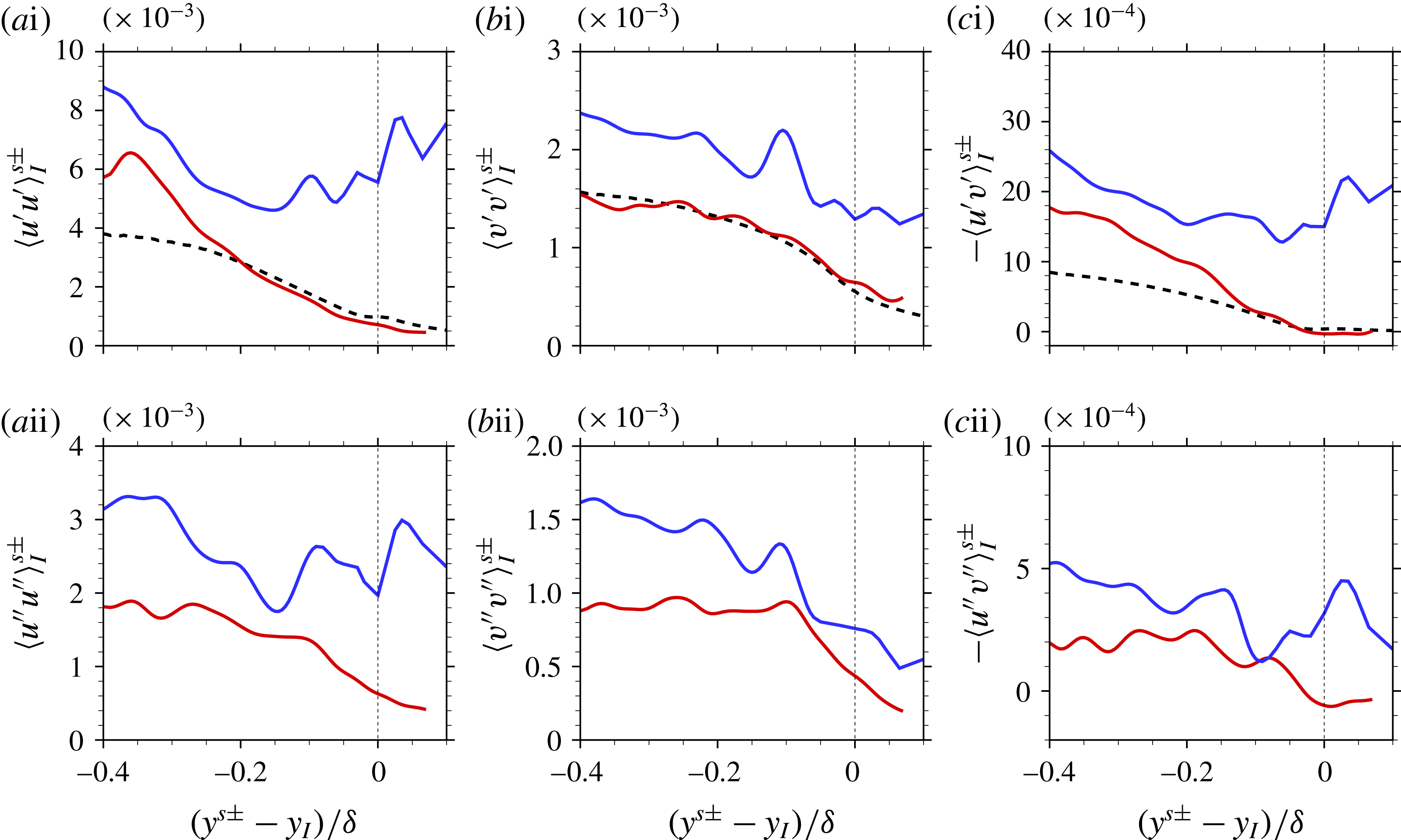
Reference Ishihara, Ogasawara and Hunt2015), which was interpreted as a viscous effect of the superlayer. Another interpretation is provided here based on the population and the intensity of the LSM. Figure 12(
 $a$
i–
 $c$
i) shows the conditional average
 $\langle u_{i}^{\prime }u_{j}^{\prime }\rangle _{I}^{s\pm }(y^{s\pm }-y_{I})$
, where the perturbations are evaluated relative to
 $\langle u_{i}\rangle _{I}$
. The spanwise stress is not shown because the spanwise perturbation is negligible at the centre of the LSM which is induced by counter-rotating streamwise roll cells (Hwang et al.
Reference Hwang, Lee, Sung and Zaki2016). All components of the conditional stresses at the cores of LSMs are generally stronger than their unconditional counterparts (dashed lines in the figure). The streamwise stress (figure 12
 $a$
i) shows stronger turbulence activity at the cores of the low-speed structures in comparison with the high-speed structures. Local averaging samples both low- and high-speed structures, as well as non-turbulent free-stream fluid that is engulfed into the boundary layer. In the present case, only the turbulent events are included. In addition, since the focus is placed on the T/NT interface, statistics are computed relative to the interface location. As a result, only high-speed events contribute appreciably to the stresses in the immediate vicinity of the interface. The wall-normal stress (figure 12
 $b$
i) conditioned on a high-speed event shadows the unconditional quantity, with the stress from low-speed events being dominant away from the interface. The unconditional Reynolds shear stress (dotted line in figure 12
 $c$
i) has a small negative value near the interface. However, the shear stress conditioned on a high-speed event remains positive value due to the finite strength of the sweep motion.
Conditional average of the turbulent stress at the LSM core.
 $Re_{\unicode[STIX]{x1D70F}}=1000$
. Reynolds (
 $a$
) streamwise, (
 $b$
) wall-normal and (
 $c$
) shear stress. (i) Velocity fluctuations relative to
 $\langle u_{i}\rangle _{I}$
and (ii) relative to
 $\langle u_{i}\rangle _{I}^{s\pm }$
. (Blue) Low- and (red) high-speed structures. The number of samples is larger than
 $1000$
at each
 $y$
-position. Dashed line indicates
 $\langle u_{i}^{\prime }u_{j}^{\prime }\rangle _{I}$
.

The conditional turbulence stresses are re-evaluated relative to the conditional mean velocity
 $\langle u_{i}\rangle _{I}^{s\pm }$
in figure 12(
 $a$
ii–
 $c$
ii), and exhibit similar trends as those in figure 12(
 $a$
i–
 $c$
i). Note that the velocity perturbation in
 $\langle u_{i}^{\prime \prime }u_{j}^{\prime \prime }\rangle _{I}^{s\pm }(y^{s\pm }-y_{I})$
is defined as
 $$\begin{eqnarray}u_{i}^{\prime \prime }=u_{i}-\langle u_{i}\rangle _{I}^{s\pm }.\end{eqnarray}$$
The results demonstrate that
 $\langle u_{i}^{\prime \prime }u_{j}^{\prime \prime }\rangle _{I}^{s\pm }$
is smaller than
 $\langle u_{i}^{\prime }u_{j}^{\prime }\rangle _{I}^{s\pm }$
. The reduction in the stress when the perturbation is measured relative to a different mean can be explained using figure 11(
 $a$
i). The markings ‘A’ and ‘B’ on the figure show an example of the moments relative to
 $\langle u\rangle _{I}$
and
 $\langle u\rangle _{I}^{s\pm }$
, at
 $(y^{s\pm }-y_{I})=0.3\unicode[STIX]{x1D6FF}$
. The latter is clearly smaller, and the more accurate measure which is reported in figure 11(
 $a$
i). Note that Kwon et al. (Reference Kwon, Hutchins and Monty2016) also remarked the importance of appropriately defining the mean profile in the computation of the turbulence stress in the intermittent region. Although the magnitude of the conditional turbulence stress can be affected by the choice of reference velocity, the current results clearly show that the stress in the low-speed event is stronger than the high-speed counterpart.
In general, the profiles of the Reynolds stresses due to the high-speed motion shadow the unconditional average near the interface. On the other hand, away from the interface, it is the Reynolds stresses due to the low-speed motion that contributes most to the unconditional average. Interpretation of the statistics based on the large scales is analogous to the attached eddy hypothesis (Townsend Reference Townsend1976), which anticipates the turbulence statistics using the intensity function and the probability of the large-scale structures. Here, however, the statistics were examined from the perspective of an observer located at the T/NT interface.
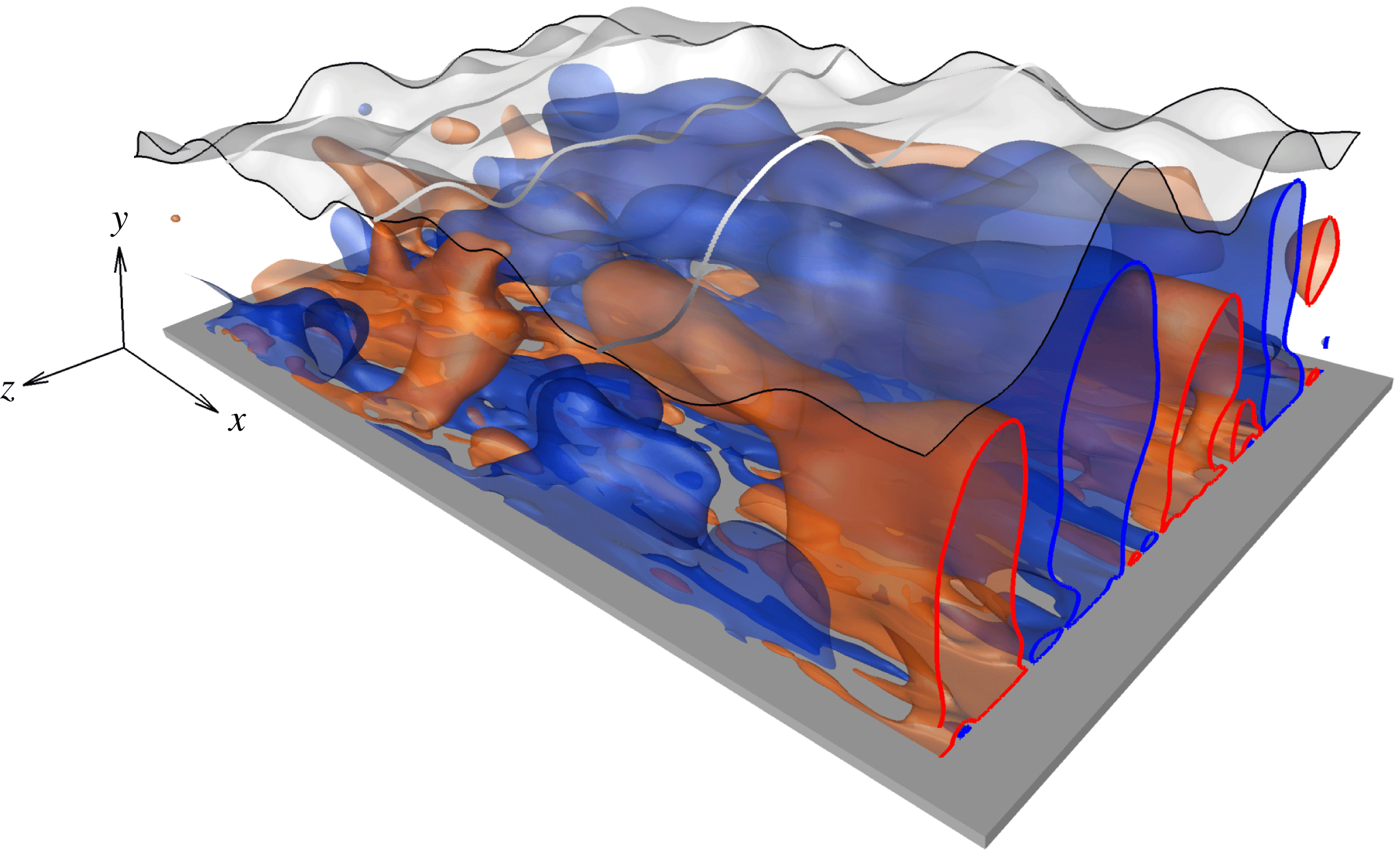
Large-scale deformation of the T/NT interface (white) and the underlying large-scale turbulent motions. Blue and red represent the low- and high-speed structures, respectively.

4 Summary and conclusions
The present study focused on the influence of LSM in a TBL at
 $Re_{\unicode[STIX]{x1D70F}}\simeq 1000$
on the T/NT interface and the near-interface statistics. Using a database of three-dimensional flow fields from DNS, the LSM was identified using a streak detection algorithm. The T/NT interface was identified using a vorticity threshold, which separates the vortical fluid motion within the boundary layer from the free stream. A summary of the results using the present criterion is presented.
The T/NT interface was first characterized by evaluating statistics of its height and fluctuations. Spectral analysis of the fluctuations showed progressively higher contribution in the wide spanwise modes with increasing Reynolds number. The spanwise dimension of the interface deformation is of the order of the local boundary-layer thickness. The two-point correlation confirms these results. It also predicts that the streamwise length scale of the interface deformations increases with Reynolds number, similar to the downstream elongation of LSMs in TBLs.
Conditional statistics provide evidence that the large scales modulate the interface height. Although both low- and high-speed structures are associated with strong turbulence activity, only the low-speed LSMs elevate the interface. The crest in the interface shape resembles the inclined shear layer associated with the low-speed LSM. On the other hand, since high-speed LSMs are associated with sweeps, they tend to lower the interface. In contrast to the shape of the LSM, the resulting valley in the interface shape has a negative inclination angle above at the location of maximum sweep.
The abrupt changes in turbulence statistics reported by previous studies were herein examined by evaluating the influence of large-scale structures on the flow field near the interface: a perspective which is consistent with the attached eddy hypothesis. The low-speed large-scale structures in the intermittent region yield a quantitatively slower mean velocity and stronger turbulent stresses than the high-speed counterparts. Figure 13 and movie 2 provide a representative visualization of the T/NT interface and the LSM in the TBL. The deformation of the interface captures its larger vertical separation from the low-speed structure, which weakens the contribution of low-speed events to the near-interface statistics. In addition, the rapid drop in turbulence stresses near the interface is coincident with the absence of the low-speed structures in that region.
The current study contrasted the effect of low- and high-speed LSMs on the deformation of the T/NT interface and on the near-interface turbulence statistics. The focus was placed on canonical zero pressure gradient TBL. Whenever the boundary layer is subjected to external forcing that alters the LSMs, the near-interface dynamics should also be reassessed. Future work should therefore examine the effects of changes in flow conditions, for example due to external pressure gradients or curvature.
Acknowledgements
This work is sponsored by the National Science Foundation (grant no. 1605404) and the Office of Naval Research (grant no. N00014-16-1-2542).
Supplementary movies
Supplementary movies are available at https://doi.org/10.1017/jfm.2017.170.
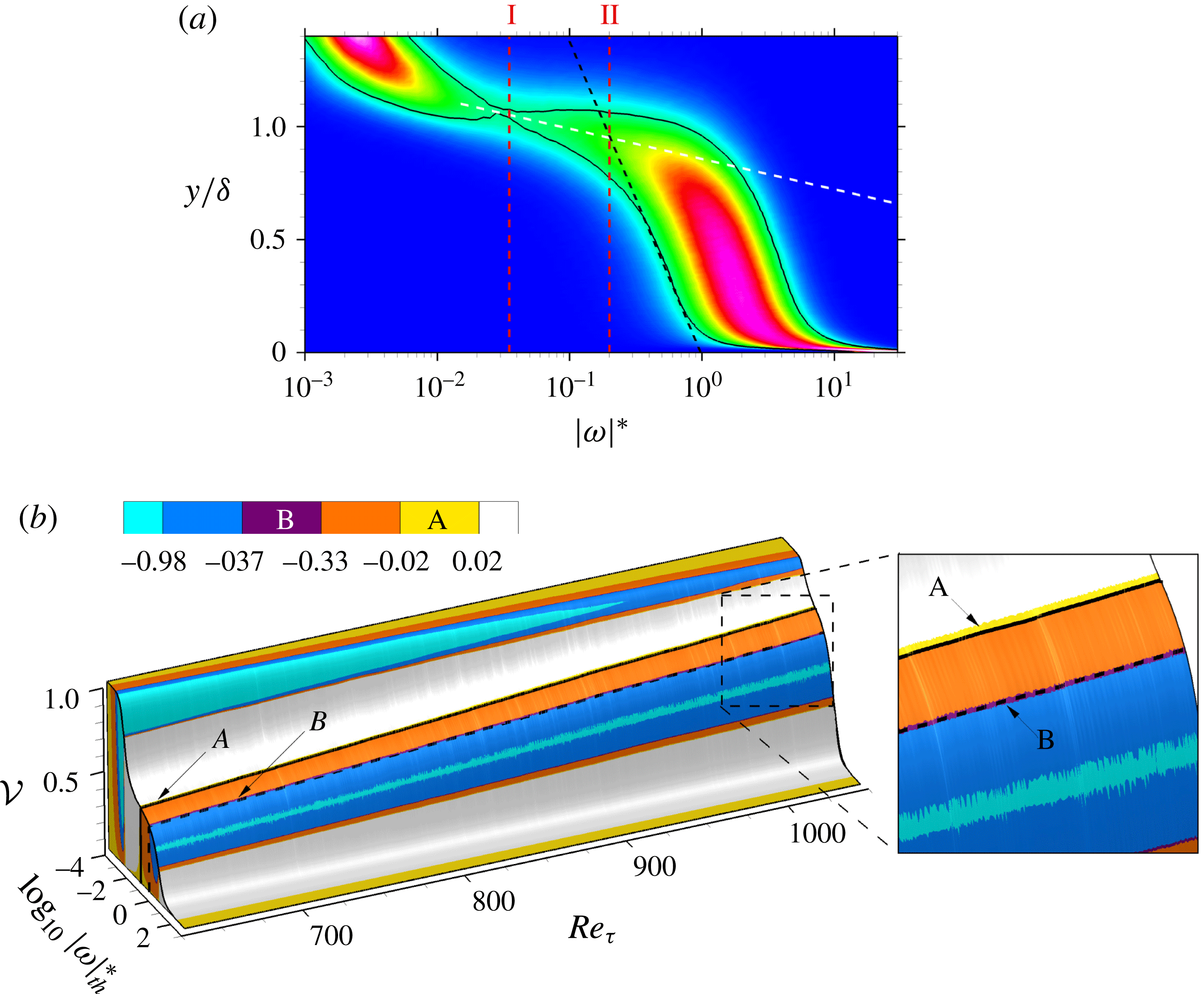
Appendix A. Volume of the vortical region
(
 $a$
) Probability density function of
 $\log _{10}|\unicode[STIX]{x1D714}|^{\ast }$
at
 $Re_{\unicode[STIX]{x1D70F}}=1000$
. Vertical lines (‘I’ and ‘II’) denote constant values of
 $|\unicode[STIX]{x1D714}|_{th}^{\ast }=0.035$
and
 $0.2$
. Definitions of black and white dashed lines follow figure 2(
 $a$
). (
 $b$
) Turbulent volume fraction as a function of the normalized vorticity magnitude. Colour indicates the second-order derivative of the volume fraction normalized by its minimum value. Black solid and dashed lines denote constant values of
 $|\unicode[STIX]{x1D714}|_{th}^{\ast }=0.035$
and
 $0.2$
.

In addition to the p.d.f. of
 $\log _{10}|\unicode[STIX]{x1D714}|^{\ast }$
(§ 2.2.1), the profile of the vortical fluid fraction is one of the often adopted measures for selection of the vorticity threshold (da Silva et al.
Reference da Silva, Hunt, Eames and Westerweel2014). The vortical fluid fraction
 ${\mathcal{V}}(|\unicode[STIX]{x1D714}|_{th}^{\ast })$
can be defined as
 $$\begin{eqnarray}\displaystyle {\mathcal{V}}(|\unicode[STIX]{x1D714}|_{th}^{\ast };~x) & \equiv & \displaystyle \frac{\displaystyle \int _{t_{0}}^{t_{0}+\unicode[STIX]{x0394}T}\int _{0}^{L_{z}}\int _{0}^{L_{y}}\unicode[STIX]{x1D6FC}\unicode[STIX]{x0394}x\,\text{d}y\,\text{d}z\,\text{d}t}{\unicode[STIX]{x0394}T~L_{z}~L_{y}~\unicode[STIX]{x0394}x},\quad \text{where }\unicode[STIX]{x1D6FC}=\left\{\begin{array}{@{}ll@{}}1 & \text{if }|\unicode[STIX]{x1D714}|^{\ast }\geqslant |\unicode[STIX]{x1D714}|_{th}^{\ast },\\ 0 & \text{if }|\unicode[STIX]{x1D714}|^{\ast }<|\unicode[STIX]{x1D714}|_{th}^{\ast },\\ \end{array}\right.\end{eqnarray}$$
 $$\begin{eqnarray}\displaystyle & = & \displaystyle \frac{1}{L_{y}}\int _{0}^{L_{y}}\unicode[STIX]{x1D6FE}(y;|\unicode[STIX]{x1D714}|_{th}^{\ast },x)\,\text{d}y,\end{eqnarray}$$
where
 $L_{y}$
and
 $L_{z}$
are the wall-normal and the spanwise sizes of the computational domain, and
 $\unicode[STIX]{x1D6FE}$
is the mean intermittency. The relationship between the two approaches, the p.d.f of
 $\log _{10}|\unicode[STIX]{x1D714}|_{th}^{\ast }$
and
 ${\mathcal{V}}$
, is demonstrated in figure 14. Note that the surface
 ${\mathcal{V}}(|\unicode[STIX]{x1D714}|_{th}^{\ast })$
in figure 14(
 $b$
) is coloured by the second-order derivative,
 $\unicode[STIX]{x2202}^{2}{\mathcal{V}}/\unicode[STIX]{x2202}(\log _{10}|\unicode[STIX]{x1D714}|_{th}^{\ast })^{2}$
, which is normalized by its minimum value. First, the minimum in the p.d.f. of the vorticity magnitude (marked ‘I’ in figure 14
 $a$
) corresponds to
 $|\unicode[STIX]{x1D714}|_{th}^{\ast }=0.035$
. In the vortical fluid fraction, the line contour of
 $|\unicode[STIX]{x1D714}|_{th}^{\ast }=0.035$
(black solid in figure 14
 $b$
) collapses onto the band for zero curvature,
 $\unicode[STIX]{x2202}^{2}{\mathcal{V}}/\unicode[STIX]{x2202}(\log _{10}|\unicode[STIX]{x1D714}|_{th}^{\ast })^{2}\approx 0$
(marked ‘A’; yellow band in figure 14
 $b$
) across the entire Reynolds number range. This criterion has been chosen as a suitable threshold in free shear flows. Second, the threshold of the current study
 $|\unicode[STIX]{x1D714}|_{th}^{\ast }=0.2$
(marked ‘II’ in figure 14
 $a$
) is the black dashed line in figure 14(
 $b$
). This threshold corresponds to approximately the normalized
 $\unicode[STIX]{x2202}^{2}{\mathcal{V}}/\unicode[STIX]{x2202}(\log _{10}|\unicode[STIX]{x1D714}|_{th}^{\ast })^{2}=-0.35$
(marked ‘B’; purple band in figure 14
 $b$
), between the plateau associated with the outer intermittent region (yellow band) and the boundary-layer wake regime (cyan band). The threshold
 $|\unicode[STIX]{x1D714}|_{th}^{\ast }=0.2$
(black dashed line) traces the constant value
 $\unicode[STIX]{x2202}^{2}{\mathcal{V}}/\unicode[STIX]{x2202}(\log _{10}|\unicode[STIX]{x1D714}|_{th}^{\ast })^{2}=-0.35$
across the entire Reynolds number range.
Appendix B. Conditional statistics for higher
 $|\unicode[STIX]{x1D714}|^{\ast }$
-threshold

Several previous studies adopted higher threshold level for the boundary-layer flow (e.g. Bisset et al.
Reference Bisset, Hunt and Rogers2002; Ishihara et al.
Reference Ishihara, Ogasawara and Hunt2015), which places the interface deeper inside the boundary layer. Corrsin & Kistler (Reference Corrsin and Kistler1955) placed their interface near
 $\overline{y_{I}}\approx 0.8\unicode[STIX]{x1D6FF}$
at
 $Re_{\unicode[STIX]{x1D703}}\approx 900$
, and Chauhan et al. (Reference Chauhan, Philip and Marusic2014a
) placed their T/NT interface near
 $\overline{y_{I}}\approx 0.67\unicode[STIX]{x1D6FF}$
at
 $Re_{\unicode[STIX]{x1D70F}}=14\,500$
. It is important to caution, however, that an artificially high threshold can place the interface through some of the internal high-shear regions within the boundary layer, which border the uniform momentum zones. In addition, such placement will affect the conditional turbulence statistics.
Same as figure 11 but
 $|\unicode[STIX]{x1D714}|_{th}^{\ast }=0.5$
.

Same as figure 12 but
 $|\unicode[STIX]{x1D714}|_{th}^{\ast }=0.5$
.

The influence of a higher vorticity threshold,
 $|\unicode[STIX]{x1D714}|_{th}^{\ast }=0.5$
, on the conditional mean velocity and turbulent stresses is reported in figures 15 and 16. The mean interface height is placed at
 $\overline{y_{I}}\approx 0.83\unicode[STIX]{x1D6FF}$
. In general, the statistics near the detected interface are qualitatively similar to the results from the lower threshold (figures 11 and 12). However, relatively larger gradients are observed near the T/NT boundary, which is consistent with the comparison of flow statistics near internal shear layers relative to the T/NT interface reported by Eisma et al. (Reference Eisma, Westerweel, Ooms and Elsinga2015).