

1. Introduction
It is more or less universally recognized that the marginal dollar of consumption generates a greater increase in welfare – or well-being, or quality of life – for an individual with relatively low income than for an individual with relatively high income, a phenomenon referred to as “diminishing marginal utility of income.” Conventional benefit–cost analysis (BCA) measures impacts in terms of dollars rather than welfare, so that, as a measure of aggregate individual welfare, it places too little weight on impacts affecting lower-income individuals and too much weight on impacts affecting higher-income individuals. In other words, conventional BCA assigns a smaller dollar value to a given increment of welfare when it accrues to a lower-income individual than when it accrues to a higher-income individual. Thus, as a measure of the welfare impact of a policy on the various affected groups, BCA is biased against the poor.Footnote 1
Utility weighting is an attempt to overcome the bias in a theoretically and empirically grounded way.Footnote 2 Many of the conceptual issues involved in utility weighting are addressed in Acland and Greenberg (Reference Acland and Greenberg2023a). It is not the goal of this article to defend utility weighting against its various detractors. Rather, this article contributes to the ongoing effort to establish rigorous methods for conducting utility weighting, address various sources of bias that can arise in the conduct of utility weighting, and expand the range of real-world settings in which utility weighting can be conducted.
To date, the literature on applications of utility weighting has been thin. Farrow (Reference Farrow2015), (Reference Farrow2023), and (Reference Farrow2024) use data on costs and benefits in bins of income, using methods that my coauthors and I have shown to be biased, potentially significantly so. Several studies in the environmental and disaster management literatures, as well as the Federal Emergency Management Agency, apply weights at the state, county, or census tract level, a method that suffers from the same biases as the binned method.Footnote 3 An extensive literature on the “weighted cost of carbon,” reviewed in Nurmi and Ahtiainen (Reference Nurmi and Ahtiainen2018), does essentially the same thing, applying weights at the country or regional level in Integrated Assessment Models.
Two articles that I am aware of apply weights to individual households using microdata, using a method that shares some of the features of the method I use in this article. Nurmi and Ahtiainen (Reference Nurmi and Ahtiainen2018) apply weights to willingness to pay values from contingent valuation surveys, but do not address all sources of bias. Hahn & Muller (Reference Hahn and Muller2023) come as close to my method as any other study in the literature, applying weights to households in census data, but failing to address some of the sources of bias. The method I use, developed in Acland and Raphael (Reference Acland and Raphael2025), goes beyond Hahn & Muller by using what Acland and Raphael refer to as “synthetic populations” and “impact proxies” to compute what they call “population weights,” as I explain below.
All of these studies use pre-tax and pre-transfer income, and none of them adjusts household income to account for household composition (so-called equivalization). Both of these omissions cause bias in favor of the poor. All of the studies that use data in income bins assign a weight to each bin that is based on some measure of the midpoint of the bin, usually average income within the bin, or the midpoint of the bin, while studies that assign weights to geographical units assign weights based on average or median income in each geographic unit. In both cases, the method of computing weights introduces an upward bias to the weights. All of these issues are addressed in Acland and Greenberg (Reference Acland and Greenberg2025), which also uses binned data, but applies novel methods to overcome these various sources of bias.
Reliance on binned or geographic-unit data results in two additional sources of bias which, to the best of my knowledge, cannot be addressed using binned or geographic data, both of which I address in a later section. These biases can be addressed by using microdata. This typically requires some approximating assumptions, as it is typically necessary to use data that do not represent the actual affected populations, but that can plausibly be treated as approximately representative of the affected populations.
To date, the only application of utility weighting that uses microdata and addresses all of the known sources of bias is Acland and Raphael (Reference Acland and Raphael2025), which applies weights to the costs and benefits of a proposed product safety rule of the Food and Drug Administration. In that article, the authors develop a set of methods for use with microdata that overcome all of the sources of bias that have been identified in existing studies and that, they argue, expand the range of feasible real-world applications of utility weighting. A key feature of this method is that it uses microdata, but in a way that extends the range of applications beyond what is possible in the existing studies that use microdata.
In this article, I apply these methods to another real-world regulation, one that affects a number of populations: a rule of the Administration for Children and Families (AFC) which, inter alia, provides salary and benefits increases to the staff of Head Start preschool programs.Footnote 4 This rule, and another which appears in an appendix, provide opportunities to explore a range of applications of weighting with microdata, in an effort to explore the feasibility of utility weighting in the real-world. The method is not new, but this article dramatically expands the range of impacts to which the method has been applied, and addresses a number of practical challenges that arise in the process of identifying and making use of appropriate data. I believe that the article will provide practitioners with the insights and guidance necessary to be able to apply the method in their own analysis.
2. Method
I begin with a brief presentation of the basic weighting method, which has been in currency for several decades. More detail can be found in Acland and Greenberg (Reference Acland and Greenberg2023a) and (Reference Acland and Greenberg2025). Standard practice is to derive the weight function (utility weight as a function of income) from an iso-elastic utility function, which is a classic and very widely used concave utility function: utility goes up with income, but more slowly as income goes up. The weighting function derived from this model is,

where
$ \varepsilon $
 is the income elasticity of marginal utility of income (the percent reduction in marginal utility of income caused by a 1% increase in income),
$ {w}_i $
 is the weight at income level
$ {y}_i $
 , and
$ {y}_m $
 is the median income. When these weights are multiplied by an individual’s willingness to pay(accept) for the benefits(costs) of a policy, the result can be thought of as the willingness to pay that they would have if they had income equal to the median.
At very low(high) incomes, the weights become very large(small), which can result in situations in which weighted net benefit is so heavily dominated by impacts at the very bottom of the income distribution that the welfare of the majority of the population is rendered essentially irrelevant. Acland and Greenberg (Reference Acland and Greenberg2025) have proposed a solution to this problem, which is to set thresholds on the weights. I currently use thresholds of
$ 5 $
 at the lower end of the income distribution and
$ \frac{1}{5} $
 at the upper end, which obtain, in the United States, at equivalized household income of approximately $15,000 and $149,000, respectively. This allows for sensitivity analysis using
$ k $
 and
$ \frac{1}{k} $
 for a range of values of
$ k $
 . My choice of
$ k=5 $
 is arbitrary. Some consensus among analysts is called for. I explore the effect of this parameter in sensitivity analysis.
Most applications of utility weighting use data on the proportion of the total unweighted value of any given impact (cost or benefit) that accrues to different bins of the income distribution of some affected population, often, but not always, quintiles.Footnote 5 The method typically used is that which is provided in the 2023 version of Circular A-4 (OMB, 2003b) (now rescinded by the Trump administration, but available in the National Archives) and in the U.K. Green Book (HM Treasury, 2022). First, multiply the proportion of impact for each bin by the total, unweighted impact to get the unweighted impact per bin. Then compute some measure of the midpoint of each bin – whether median or average income within the bin or just the midpoint between the upper and lower bounds of the bin – and compute the weight at that midpoint. Multiply the unweighted impact for each bin by the weight for the bin and sum over bins.
For example, suppose the bins are quintiles of the distribution of income in some affected population, that median income in the first quintile is $25,000 and members of that quintile are predicted to experience 15 % of the total unweighted benefit, that the total unweighted benefit is predicted to be $10 million and that median income in the population as a whole is $45,000. First one computes the weight at $25,000. With the value of
$ \varepsilon =1.4 $
 recommended by the 2023 Circular A-4, the weight for the bin is 2.28. Then one multiplies the total unweighted benefit (estimated in the unweighted BCA) by .15 to get the unweighted benefit on the first quintile, $150,000. Then one multiplies that number by the weight, to get the weighted benefit on the first quintile, $342,000. Repeat for the other four quintiles and sum over quintiles.
Acland and Greenberg (Reference Acland and Greenberg2025) have identified a number of limitations of this simple method. Bias is introduced by not accounting for the effect of the tax and transfer system or the effect of household composition on household income. Bias can also result from assigning weights to bins using bin-midpoint income. Acland and Greenberg provide solutions to these problems, but two other, potentially serious issues cannot be addressed using binned data: first, the possibility that either income or per-person cost or benefit may be non-uniform within bins, and second, the possibility that household composition may differ between different affected populations. The reader is referred to Acland and Greenberg (Reference Acland and Greenberg2025) for details of each of these issues. It is also the case that more often than not, binned data on affected populations is not available.
The solution to these challenges proposed by Acland and Raphael (Reference Acland and Raphael2025) – and used in this article – is to use microdata. Not only does the use of microdata overcome all of the problems identified in Acland and Greenberg (Reference Acland and Greenberg2025), when combined with the method developed by Acland and Raphael, it also significantly expands the range of potential applications of utility weighting. Microdata on the income, household composition and per-person cost or benefit is rarely available for specific affected populations, but Acland and Raphael demonstrate that it is possible in many cases to identify a subset of an existing dataset that can plausibly be treated as representative of the affected population – what Acland and Raphael call a “synthetic population” – and to find, in the data, some proxy for per-person cost or benefit that can plausibly be treated as proportional to the actual cost or benefit of the policy under analysis.
Acland and Raphael refer to their method as “population weighting.” Rather than computing the actual utility-weighted cost or benefit to an affected population, one computes the ratio of the total utility-weighted cost or benefit to total unweighted cost or benefit. This number is referred to as the “population weight” for the specific cost or benefit to the specific population. Multiplying this population weight by the total unweighted cost or benefit to the affected population, computed in the BCA to which utility weights are being applied, gives an estimate of the total utility-weighted cost or benefit.
Here is the math, followed by two illustrative examples. Let
$ {V}_i $
 be the true unweighted cost or benefit of some policy to individual
$ i $
 . Let
$ {P}_i $
 be the value of some proxy for the unweighted cost or benefit to individual
$ i $
 , and let
$ \rho $
 be some coefficient of proportion that is common across individuals, such that
$ {V}_i=\rho \bullet {P}_i $
 . For example, suppose
$ {V}_i $
 is the cost of regulatory compliance borne by an individual shareholder in a regulated firm, and that
$ {P}_i $
 is the market value of shares in regulated firms held by individual
$ i $
 . Then
$ \rho $
 is the cost of compliance per dollar of shareholdings, which is assumed to be constant across individuals. Similarly, suppose
$ {V}_i $
 is the dollar value of benefits that accrue to a household that has children in Head Start programs, and that
$ {P}_i $
 is the number of such children in the household. Then
$ \rho $
 is the dollar value of benefits per child.
The population weight on a particular cost or benefit to a particular affected population is the ratio of the total weighted cost or benefit to the entire affected population to the total unweighted cost or benefit to the entire affected population. If
$ {w}_i $
 is the weight on household
$ i $
 , then the total weighted cost or benefit to the affected population will be
$ \sum \limits_i{w}_i\bullet {V}_i=\sum \limits_i{w}_i\bullet \rho \bullet {P}_i=\rho \bullet \sum \limits_i{w}_i\bullet {P}_i $
 , and the total unweighted cost or benefit will be
$ \sum \limits_i{V}_i=\sum \limits_i\ \rho \bullet {P}_i=\rho \bullet \sum \limits_i{P}_i $
 . In the ratio that comprises the population weight,
$ \rho $
 drops out, so that the population weight,
$ W $
 is,

Again,
$ W $
 , the population weight, is the ratio of weighted to unweighted cost or benefit, or the weighted cost or benefit as a proportion of unweighted cost or benefit. If
$ C $
 is the total unweighted cost or benefit computed in the unweighted BCA to which utility weighting is being applied, then
$ W\times C $
 provides an estimate of the weighted cost or benefit. Table 1 lists the parameters involved in these computations.
Population-weighting parameters

Table 1. Long description
The table consists of two columns: Parameter and Definition.
* V sub i: Unweighted cost or benefit to individual i.
* P sub i: Proxy for unweighted cost or benefit to individual i.
* rho: Proportion of V sub i represented by P sub i.
* w sub i: Utility weight on individual i.
* W: Population weight on the cost or benefit to the affected population.
* C: Total unweighted cost or benefit across the affected population.
* W times C: Total weighted cost or benefit across the affected population.
To be valid, a proxy must satisfy the following requirements: (a) it must be observable at the individual or household level in the available microdata; (b) it must be plausible that the proxy is proportional to the actual dollar value of the impact – which is to say that the actual dollar value is the proxy multiplied by some (unobserved) term,
$ \rho $
 , that can be plausibly assumed to be constant across individuals or households.
It turns out that in many cases, with some (hopefully publicly available) microdata, some creativity, and some plausible assumptions (of the sort that are routinely made in unweighted BCA), population weights can be computed. This brings me to the two case studies referred to in the introduction. The first appears in the next section. The second is available as Supplementary Material.
3. Head Start case study
In 2024, the Administration for Children and Families (ACF) promulgated a rule that is expected to result in salary increases in Head Start-funded preschool programs, along with increased break time and fringe benefits.Footnote 6 The rule includes several additional components having to do with behavioral health provision, lead abatement, and eligibility criteria, among other things. (For the sake of clarity, I will refer to the Head Start program itself as “Head Start,” and actual preschool programs that are funded by Head Start – and thus bound by its rules – as “Head Start programs.”) The ACF, in its Regulatory Impact Assessment (RIA), estimated total expenditures on salary increases, break time, fringe benefits and a component of the rule referred to as “wage compression,” which allows programs to increase salaries for non-teaching staff to maintain internal pay hierarchies.
The RIA provided qualitative assessments of additional, unquantified benefits to workers and to children who attend Head Start programs, who I will refer to as “participants.” Thus, there are four affected populations: taxpayers, teaching staff, non-teaching staff and households with participant children, which I will refer to as “participant households.” I will present my method for each of these populations, focusing first on the synthetic population and then on the impact proxy.
3.1. Taxpayers
3.1.1. Synthetic population
The IRS has data on the actual population of taxpayers, but access to the data is severely restricted.Footnote 7 Access is given to academics but requires an extensive application process. (A separate study utilizing this data would allow for a more robust estimation of the population weight for federal taxation, which could be used widely in other studies.) Organizations such as the Tax Foundation and the Congressional Budget Office (CBO) make binned data available, but my goal is to reap the advantages of using microdata. One option, which I did not pursue, would be to start with Current Population Survey (CPS) data, which has more detailed information on household income, and feed the data into the National Bureau of Economic Research’s tax simulator, TAXSIM, to get a close approximation of the tax paid (or received, if tax credits lead to payments from the government) by each household in the dataset. This is an arduous process, and though I believe it would not be out of reach for some well-resourced agencies, I use a more straightforward, if less granular, option that uses the American Community SurveyFootnote 8 (ACS). Not all adults in the ACS pay taxes, but my proxy is based on average effective tax rate at different income levels, so assigning the average to all members of the population at any given income level allows me to use the entire adult population in the ACS as a synthetic sample.
3.1.2. Impact proxy
In the absence of information on the actual tax burden, or effective tax rate, for each household, I make use of data from CBO on the effective tax rate at different levels of the distribution of equivalized income. They report the average effective tax rate for each of the first four quintiles and then for the 81st–90th percentiles, 91st–95th, 96th–99th and then the top one per cent. I assign these effective tax rates to households in ACS data according to their place in the distribution of equivalized income and multiply by total household income. That number is my impact proxy. I do not know the actual cost of the program to each individual taxpayer, but I can plausibly assume that it is proportional to each individual’s total tax burden. (In some sense it has to be, because the money that funds the program is taken from the total pot of tax revenue, which is an undifferentiated mix of revenue from each tax-paying household.)
This approach has the unfortunate property of relying on binned data for one part of the process. The fact that the burden of taxation is actually increasing within each of the bins imparts an upward bias to the population weight on taxpayers. We shall see that this is actually a desirable bias, because the weighted benefit–cost ratio is above 1, so having an upward-biased estimate of weighted cost does not change the result qualitatively.Footnote 9
Summary.
Ideal data:
-
• Actual household tax burden, household income and household composition for all taxpayers.
Synthetic population:
-
• ACS 5 % sample, all adults not in group quarters.
-
• Assumes income and household composition are the same, within quintiles, among taxpayers as in the population as a whole.
Impact proxy:
-
• Average effective tax rate by quintile, with top quintile broken down more finely.
-
• Applying average rate to all adults is mathematically the same as identifying actual taxpayers and using their individual effective tax, under the assumption that income and household composition are the same among taxpayers as in the population as a whole.
-
• Assumes that household composition is constant across the income distribution within quintiles.
3.2. Teaching staff
3.2.1. Synthetic population
The National Survey of Early Childhood Education (NSECE) has a teacher survey, which includes an indicator for whether the program an individual teaches at is funded by Head Start. (A program is bound by the rules of Head Start if even a portion of its funding comes from Head Start.) However, income is top-coded at $60,000, making the data inadequate for utility weighting. Instead, I again use ACS data. I construct a synthetic population as follows.
First, in NSECE data, I identify five covariates that differ significantly between Head Start and non-Head Start teachers and that are correlated with income, so that a population that was representative of Head Start teachers on those covariates would likely be approximately representative with respect to income. The five characteristics are marital status, educational attainment (below or above the associate’s degree level), White or non-White, age (in three categories) and whether the teachers’ household received some kind of government assistance. Each of these is a categorical variable. I could have chosen more variables or more categories of each variable, but the number of teachers in each subcategory in the NSECE data would have gotten too small to be statistically reliable.
I create a categorical variable that has a separate value for each of the five-way intersections of the five categorical covariates, resulting in 48 categories. For example, a married, white individual in the lowest age category, with a bachelor’s degree, receiving government assistance would be in one category, and so forth. I then compute the frequency distribution of these categories among Head Start teachers – applying sample weights – identify the modal category, and compute the frequency in each category as a proportion of frequency in the modal category. Thus, if the modal category is the one mentioned above and there are 15,000 individuals in this category in NSECE data, and 7,500 individuals in some other category, that other category would be assigned a proportional frequency of .5. I use these proportions to select individuals in ACS data in the same proportions, as follows.
First I go into ACS data and identify individuals in teaching occupations in the childcare industry, which includes preschools and daycare centers. I assume, I believe innocuously, that individuals identified as having a teaching role are more likely to work in preschools than in daycare centers. I create the same categorical variable as in the NSECE data and select, for my sample, all of the individuals in the category that was the modal category in the NSECE data. I then randomly add to my sample, from each category, a number of individuals equal to the number in the modal category multiplied by the proportion computed for that category, as calculated above. (Sample weights from the ACS are applied throughout this procedure.)
A simplified example will help demonstrate. Suppose there were three categories of Head Start teachers in the NSECE data, 1, 2 and 3, and suppose that the sample-weighted number of teachers in the three categories in the NSECE data was 50, 75 and 100 respectively. I convert their frequencies to proportions of the modal category, so that the proportions are .5, .75 and 1, respectively. In ACS data, I find that there are, let us say, 200 teachers in category three and select all of them for my synthetic sample to maximize the size of the sample. Then, I identify teachers in category 2 and randomly select .75 × 200 = 150 of them, and then .5 × 200 = 100 of the teachers in category 1. Again, I apply sample weights throughout.
What I am left with is a sample of individuals in teaching occupations in preschools that is representative with respect to the five selected covariates: it has the same proportions of teachers in each of the five-way intersections of the five covariates as in the NSECE data on actual Head Start teachers, which is another way of saying that it has the same joint frequency distribution, in proportional terms, as the population of teachers in the NSECE. I assume that these individuals are approximately representative of Head Start teachers, particularly with respect to work and income-related characteristics.
3.2.2. Impact proxy
To construct my impact proxy, I take advantage of the fact that the various impacts of the rule on individuals are all functions of educational attainment, wages, hours worked, and local cost of living, all of which I have, or have proxies for, in ACS data. The rule sets a target wage that teachers must earn, and ACF has computed the average target wage and average baseline wage by occupation and educational attainment. I compute the difference (the wage increase) and average across occupations for individuals with and without a college degree. I assign a benefit from wage increase to individuals in ACS by multiplying the relevant wage increase by annual hours worked.
The RIA estimates the average break time that will be gained by teachers and estimates that 20 % of programs already provide the required break time, so that, provided that the programs in that 20 % are representative of all programs with respect to the number of teachers, there is an 80 % chance that any randomly selected teacher will receive the benefit of additional break time. ACF has estimated the average number of minutes of break time that will be gained by teachers. I value this increased break time at half the baseline wage for each individual, computing wage as the ratio of income from wages to annual hours worked, under the arbitrary assumption that time spent on a break from work is half as valuable as the marginal value of time spent outside work. I assign this benefit to 80 % of individuals, at random.
The rule requires that teachers be paid a wage that is at least what ACF considers a living wage in each location, even if this wage is above the target wage set by the rule. The RIA estimates that this will have a cost equivalent to the cost of 15 % of teachers receiving a salary increase of $2. I rank Public Use Microdata Areas (PUMAs) nationally, by cost of living, and select PUMAs in descending order of cost of living until I have a set of PUMAs that contains 15 % of the population of teachers. In other words, I select the top 15 % of the distribution of cost of living across teachers. I assign a $2 wage increase to teachers in these PUMAs. I apply sample weights for this procedure.
I use a proxy for cost of living in each PUMA that I create by regressing total housing cost on household income, a dummy for ownership versus rental, the number of bedrooms, and the number of other rooms. I conduct this regression for each PUMA. I normalize bedrooms, other rooms, and household income such that the constant term for each PUMA is the total cost of housing for a median income household renting a unit with two bedrooms and two other rooms. This is my proxy for PUMA cost of living.
I use estimates of fringe benefit rates from the RIA to assign a dollar value of fringe benefit increases to each worker. Finally, I assign each household an effective marginal tax rate (EMTR, the percentage of the marginal dollar of income that does not enter the household’s budget because of taxation and decreases in eligibility for government assistance) and multiply that by my estimate of the salary increases caused by the rule to compute the reduction in salary increases caused by taxes and loss of eligibility. (In an unweighted BCA this would be ignored as it is a transfer, but in weighted BCA transfers must be accounted for.) I use estimates of EMTR by poverty level from the Office of the Assistant Secretary for Planning and Evaluation at the Department of Health and Human Services.
The sum of all of these components of benefit comprises my benefit proxy. For the most part this is an estimate of the actual dollar value of benefit to each teacher, though not in the case of break time. It is still necessary to use the population weighting method instead of computing weighted benefit directly because the number of individuals represented by my synthetic population is unlikely to be the same as the number of Head Start teachers affected by the rule.
Summary.
Ideal data:
-
• Baseline wage rate, hours worked, and break time; local area wage for k/1 teachers; local area cost of living; household income and composition.
Synthetic population:
-
• ACS 5 % sample, not in group quarters.
-
• Randomly selected subset of individuals in teaching occupations in the childcare industry that is representative of actual Head Start teachers with respect to the joint distribution of five observables that are correlated with income and differ significantly between Head Start and non-Head Start teachers in NSECE data.
-
• Assumes that population identified in ACS data by joint distribution is representative of Head Start teachers with respect to income, household composition, and baseline wage rate, hours worked, and geographic location.
Impact proxies:
-
• Average wage increase predicted by ACF by education level, multiplied by baseline annual hours worked.
-
• Predicted average break time gained per teacher multiplied by half of baseline wage rate and then multiplied by .8 to simulate the omission of teachers in programs already receiving break time.
-
• Baseline wage multiplied by average fringe rate and predicted increase in fringe benefits.
-
• Two dollars multiplied by annual work hours, assigned to individuals living in PUMAs representing the top 15 % of workers by cost of living, using a constructed proxy for PUMA cost of living based on a regression of total housing cost on observables.
-
• Assumes actual individual wage increase, baseline break time, and baseline fringe rate are not correlated with income or household composition.
-
• Assumes error in assigning individuals to high cost of living PUMAs is not correlated with income or household composition.
-
• Assumes income and household composition are the same between programs that currently give break time and those that do not.
3.3. Non-teaching staff
3.3.1. Synthetic population
ACF has data on the non-teaching staff at Head Start programs, but it is not publicly available and my attempt to acquire it was unsuccessful. Thus, once again, I begin with ACS data. To identify individuals who would be affected by the wage compression component of the rule I restrict the sample to the childcare industry, but then need to identify occupations that programs would find it necessary to provide with salary increases in response to salary increases for teaching staff. First, I used generative AI (ChatGPT 5.1) to identify a set of non-teaching occupations that could potentially be employed at Head Start programs. I then reached out to individuals within several California county governments who are responsible for overseeing Head Start within their counties. I was able to get useable input from one county. I provided them with a spreadsheet containing the list of potentially relevant occupations and asked them to rate how likely they thought it would be that each occupation would need to have their salaries increased, on a 5-point scale, where 1 was “not likely at all” and 5 was “very likely.” My contact at the county presented this spreadsheet to her staff, who collaborated on a set of responses. This left me with a list of 8 occupations with a likeliness rating of 2 or above, to which I restrict my dataset. Note that I did not attempt to find workers who are most likely to work at Head Start programs in particular. I implicitly assume that, unlike teachers, there are no significant differences between workers in these occupations who work at Head Start programs and those that work at non-Head Start programs.
3.3.2. Impact proxy
The RIA assumes that wage compression will result in expenditures equal to 10 % of expenditures on target wages and fringe benefits to teachers. It does not comment on how this expenditure will be allocated across workers. For simplicity I assume that workers will receive a percentage increase in their pay, and that the percentage increase will be constant across workers. I do not need to know what that percentage will be, only that it will be proportional to total income from wages.
For each affected occupation I divide the one-to-five likelihood rating mentioned above by 5 to get an approximation of the probability of being affected by the rule. (I realize that treating an ordinal variable as a cardinal measure is incorrect, but I believe it is an acceptable approximation.) I multiply income from wages by one minus the EMTR, as above, to reflect the fact that workers will ultimately receive less than their full salary increase due to income taxes and reduced eligibility for government support. Then, I multiply that number by the probability of being affected by the rule, described above, which is mathematically the same as randomly selecting the appropriate number of workers in each occupation and giving them the full benefit. The result is my proxy. Without knowing anything about what each individual will actually receive, under the assumption of constant percentage salary increase I can plausibly argue that my proxy is approximately proportional to the true benefit to each individual, which is what I need for a valid proxy.
Summary.
Ideal data:
-
• Baseline wage rate, wage increase, household income, and household composition for individuals actually affected by the policy.
Synthetic population:
-
• ACS 5 % sample, not in group quarters.
-
• Individuals in childcare industry working in occupations identified by a group of Head Start experts.
-
• Assumes distribution of observables for affected workers in Head Start programs is the same as in the childcare industry as a whole.
-
• Assumes error in expert identification of affected occupations is not correlated with income or household composition.
Impact proxy:
-
• Income from wages multiplied by likelihood of occupation being affected by policy, as rated by a group of Head Start experts.
-
• Assumes error in expert estimation of probability of being affected is not correlated with income or household composition.
3.4. Participant households
3.4.1. Synthetic population
In this case I have data on the actual affected population, in the form of the family survey in the NSECE. I identify affected households as those with any child who attends any program that is a Head Start program.
3.4.2. Impact proxy
I do not know the benefit per participant, but I assume that it is the same for each child, regardless of how many children are in a household, so that my proxy is simply the number of children in the household. This is a case in which I conduct my analysis at the household level rather than the individual level. The result is the same as if I had assigned a proxy of 1 to each Head Start child and used individual rather than household sample weights.
Summary.
Ideal data:
-
• Number of children in Head Start programs, household income and household composition for families with children in Head Start programs.
Synthetic population:
-
• None. Ideal data is available, with the exception of unweighted benefit for each child.
Impact proxy:
-
• Number of children in household in Head Start programs.
-
• Assumes variation in benefit per child of Head Start participation is not correlated with household income or household composition.
3.5. Results
The population weights for the relevant costs and benefits to the affected populations appear in Figure 1. Ninety five per cent confidence intervals were computed using Monte Carlo simulation, described in the section on sensitivity analysis. Note that any given population weight reflects not only the income distribution of the affected population, but also the distribution of individual cost or benefit across the income distribution. For example, the monetary benefits of the Head Start rule are a function of hours worked, hours worked is correlated with labor earnings, and the labor earnings of the individual are correlated with the income of the household they live in. Thus, mechanically, individuals with higher household income will, on average, experience a greater benefit from the rule, driving down the population weight, because the benefit falls disproportionately on individuals with relatively high household income, and thus relatively low individual utility weights.
Population weights for populations affected by Head Start rule.

This is one part of the reason that the population weight on benefit to Head Start teachers, 0.828, is so far below 1. But the weight would not be anywhere below 1, the weight at median income, if a significant number of Head Start teachers were not living in households with income above the median. In fact, the teachers in my synthetic population of Head Start teachers disproportionately live in households that include relatively high earning individuals. It is true that there are a good number of Head Start teachers living alone, with quite low incomes, but the policy is not well targeted at them, and winds up benefitting a relatively large number of people who, purely on the basis of our concern for the welfare of lower-income individuals, might not be of such great concern to advocates.Footnote 10
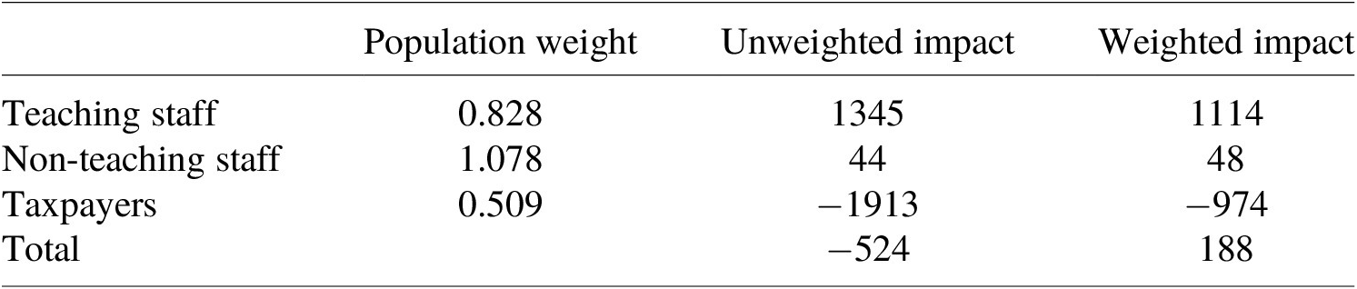
Now, one might think that when a policy is targeted at a population with a population weight below 1 unweighted BCA would actually be biased in favor of that population, but in this case, as Figure 1 reveals, the population weight on those who bear the cost of the rule, taxpayers, .509, is even smaller than the weight on teachers, because the bulk of federal taxes is paid by quite high-income households.Footnote 11 So, even though weighting drives down both cost and benefit, unweighted BCA is nonetheless biased against the population receiving the benefits. Meanwhile, the population weight on non-teaching staff (for whom the total unweighted benefit is relatively small) is 1.078.
The ACF, in its RIA, estimated the cost to taxpayers of all of the significant components of the rule, including monetary and non-monetary costs of salary and fringe-benefit increases, additional break time, and smaller costs such as the need for extra staffing to achieve reduced caseloads among social workers, and the lead abatement requirements built into the rule. The total cost computed by ACF was $1.68 billion. Some of this will come back to taxpayers in the form of income taxes and reduction in public benefits caused by decreased eligibility. Also, deadweight loss from taxation (so-called excess burden of taxation) must be included. I estimate the cost to society, when these values are accounted for, at approximately $1.91 billion.
ACF did not estimate benefits, but I have conducted a back-of-the-envelope analysis based on numbers from the RIA, and estimates of the EMTR, and find that, when the reduction in salary increase from income taxes and reduced public benefits is accounted for, the unweighted benefits to teaching and non-teaching staff are $1.35 billion and $44.3 million, respectively. Thus, the unweighted net benefit is approximately -$524 million. When population weights are applied, the weighted benefits to teaching and non-teaching staff are approximately $1.11 billion and $47.8 million, respectively, and the weighted cost to taxpayers is approximately .974 billion, leaving a weighted net benefit of approximately $188 million. Table 2 summarizes these results. Recall that the population weight on taxpayers was biased up by the fact that the distribution of tax burden within income bands is increasing with income. Without this bias the weighted net benefit would have been even greater.
Weighted and unweighted benefits and costs

Table 2. Long description
The table consists of four columns: Population category, Population weight, Unweighted impact, and Weighted impact.
* Teaching staff: Population weight 0.828, Unweighted impact 1345, Weighted impact 1114.
* Non-teaching staff: Population weight 1.078, Unweighted impact 44, Weighted impact 48.
* Taxpayers: Population weight 0.509, Unweighted impact minus 1913, Weighted impact minus 974.
* Total: Unweighted impact minus 524, Weighted impact 188.
Despite the fact that weighting deflated both costs and benefits, the effect was greater on costs, so the sign of net benefits was reversed. And, though ACF did not quantify any potential benefits that children participating in Head Start programs might receive – perhaps through increased teacher retention and attraction of higher-skilled teachers – the population weight on households with children in Head Start programs was 4.173, so that it would not take much benefit to participant households to increase the weighted net benefit considerably.
Note that while the change in sign of net benefits unambiguously tells us that the policy has net positive welfare impacts – despite failing the potential Pareto test – we cannot meaningfully say that the increase in net benefit caused by weighting is the difference between the weighted and unweighted net benefit, $748 million. The reason is that weighted and unweighted BCA are measured in different units. Both are measured in units of dollars, but a dollar’s worth of cost or benefit in unweighted BCA is based on the WTP of whoever the cost or benefit accrues to, which, for any given welfare impact, varies in value across the income distribution, whereas a dollar’s worth of cost or benefit in weighted BCA is based on the WTP of the median income individual, the value of which, for any given welfare impact, does not vary across the population. Thus, the -$560 million of unweighted net benefit and the $188 million of weighted net benefit cannot meaningfully be added to or subtracted from one another, any more than the length of an object measured in inches can be meaningfully added to or subtracted from the length of another object measured in centimeters.
What can be meaningfully compared is the weighted and unweighted benefit–cost ratios (BCRs), because in the ratio, the units of measure drop out. The unweighted BCR of the Head Start rule is .727 and the weighted BCR is 1.193, which means that unweighted BCA, were it to be taken as a measure of the welfare return on “investment,” was wrong by .466.
4. Sensitivity analysis
The results of utility weighting are sensitive to the parameters of the weighting process, most notably the income elasticity of marginal utility of income,
$ \varepsilon $
 . The empirical literature on this parameter is vast, and while meta-analyses have been conducted, these have, at best, narrowed the range of plausible values. Acland and Greenberg (Reference Acland and Greenberg2023b) found a 95 % confidence interval of approximately 1.2–2, but values well below that range continue to hold currency.Footnote
12 As
$ \varepsilon $
 gets bigger, weights above 1 get bigger and weights below 1 get smaller, pushing costs and benefits to lower-income populations up and costs and benefits to higher-income populations down.
Figure 2 shows the effect of
$ \varepsilon $
 on the population weights, and the weighted net benefit. I explore a range of values from 1 to 2. Going from the bottom to the top of that range increases the weighted net benefit by a factor of almost 3. The population weight on taxpayers goes down while those on teaching and non-teaching staff go up. It is interesting to note that while individual-level weights below 1 go down as
$ \varepsilon $
 goes up, the population weight on teaching staff goes up even though it is below 1. Population weights do not follow the same rules as individual weights. Among teaching staff, some have weights above 1 and some below, and the effect of increasing
$ \varepsilon $
 is greater in absolute terms on weights above 1 than on weights below 1, because the weight function is hyperbolic.
Sensitivity analysis on
$ \varepsilon $
 for Head Start rule.

The results might suggest that the weighting enterprise is quite fragile. What matters for policy analysis, however, is whether the variation in weighted net benefit caused by different values of
$ \varepsilon $
 is sufficient to change the ranking of policy alternatives. In this case the answer is a fairly resounding no.
My analysis includes a new feature in the weighting method, which is the thresholds I place on the weights. Intuitively, we would expect these thresholds to have a similar effect as
$ \varepsilon $
 , because relaxing the thresholds increases the weights at the bottom end of the income distribution and decreases those at the top end. Indeed, this is what Figure 3 reveals. I vary the upper threshold from 4 to 12, which has the effect of varying the lower threshold from .25 to .083. In proportional terms the effect is fairly large. Again, variation over a reasonable range of thresholds does not change the sign of weighted net benefit.
Sensitivity analysis on weight thresholds for Head Start rule.

Anytime the number of uncertain parameters and assumptions in a model increases, the range of uncertainty in the outputs of the model increases. This is no less true for weighting, which adds assumptions and parameters on top of those necessary to conduct unweighted BCA. For this reason, I conduct Monte Carlo simulations. I am not able to vary the parameters of the unweighted benefit–cost analyses, but I conduct Monte Carlo simulations on the weighted net benefit, varying each of the parameters in each of the models using a triangular distribution with min and max 25 % below and above my preferred parameter estimates. Table 3 shows the distributional parameters used in the simulation.
$ \alpha $
 and
$ \beta $
 are the parameters of the tax-and-transfer adjustment formula and are modeled as having normal distributions. All other parameters are modeled as having triangular distributions.
$ \varepsilon $
 is the income elasticity of marginal utility of income. LWP is the proportion of teachers assumed to require an increase in wage to match local cost of living. MOB is the minutes of break teachers are assumed to receive, and PWB is the proportion of teachers assumed to not currently receive break time. BWD is the wage deflator for valuing break time. Fringe 1 and Fringe 2 are the parameters used to calculate the benefit of increased fringe benefits. The ETR parameters are the effective tax rates for the eight income bins used, and the EMTR parameters are the EMTRs for the 10 deciles of the income distribution.
Distributional parameters used in Monte Carlo simulation

Table 3. Long description
The table is divided into two main sections.
1. Normal distributions section with columns for Mean and S D (Standard Deviation):
- alpha: Mean 2.1319, S D 0.01662.
- beta: Mean 0.07398, S D 0.0006813.
2. Triangular distributions section with columns for Min, Mode, and Max:
- varepsilon: Min 1.05, Mode 1.4, Max 1.75.
- L W P: Min 0.112, Mode 0.15, Max 0.187.
- M O B: Min 3786, Mode 5049, Max 6311.
- Proportion without break: Min 0.6, Mode 0.8, Max 1.
- Break wage deflator: Min 0.375, Mode 0.5, Max 0.625.
- Fringe 1: Min 0.024, Mode 0.032, Max 0.04.
- Fringe 2: Min 0.204, Mode 0.272, Max 0.34.
- E T R bins 1 through 8: Values range from E T R bin 1 (Min 0.225, Mode 0.3, Max 0.375) down to E T R bin 8 (Min 0.00375, Mode 0.005, Max 0.00625).
- E M T R d 1 through d 10: Values range from E M T R d 1 (Min minus 0.165, Mode minus 0.22, Max minus 0.275) to E M T R d 10 (Min 0.21, Mode 0.28, Max 0.35).
Figure 4 shows the results. The 95 % confidence interval is $109 million to $264 million. This is a fairly wide range, though perhaps not atypical for BCA as a whole. Again, the most important observation, from the standpoint of policy analysis, is that the confidence interval does not include zero.
Distribution of weighted net benefit from Monte Carlo simulation.

5. Conclusion
I have presented a new method for conducting utility weighting using microdata to compute what I call “population weights,” with synthetical populations and impact proxies. This method eliminates all of the known sources of bias that can arise when conducting weighting with binned income data and significantly expands the range of applications of weighting. I have applied the method to two real-world regulations for which unweighted benefit–cost analyses have been conducted.
Utility weighting deflated the monetized benefit of the Head Start rule, but by less than it deflated the burden of the rule on taxpayers, leading to an increase in the BCR from below 1 to above 1, indicating that the bias in BCA as a measure of net benefit to society was significant enough to generate what many people would consider to be an incorrect policy recommendation.
There is no doubt that conducting utility weighting of the sort I have reported in this article adds to the amount of time necessary to complete regulatory review. What I have concluded, however, is that data availability is significantly less of a concern than has been expressed to date by scholars and practitioners, most of whom have not actually conducted utility weighting, and the expertise and skills necessary to conduct the analysis are not prohibitive for many agencies and organizations.
My coauthors and I have now conducted a total of seven utility weighting analyses on real-world policies affecting a total of 17 different populations. It is my intention to write an instruction manual on the basis of these seven case studies, and the lessons we have learned in the process of conducting the analyses, as well as other existing literature. My own experience is that it can be hard to learn a new method from academic articles, and indeed, it is sometimes hard for an article that attempts to provide adequate methodological guidance to survive peer review, as reviewers and editors quite often call for significant cuts in the interest of brevity. It is my hope to provide all of the guidance that I am equipped to provide, in one place, with as much detail and explanation as necessary to enable a reasonably skilled analyst to conduct utility weighting in a range of real-world settings. The manual will be freely available at no cost.




 Open access

