Nomenclature
- BWB
-
blended wing body
- BLI
-
boundary layer ingestion
- APG
-
adverse pressure gradients
- AIP
-
aerodynamic interface plane
- Ma
-
Mach number
-
 ${D_{{\rm{out}}}}$
-
intake exit diameter
- L
-
aerofoil chord length
- L
-
distance from the upper wing surface to the intake lip
- X
-
dimensionless distance l/L
-
$DC\left( {150} \right)$
-
total pressure distortion
-
$SC\left( {150} \right)$
-
swirl distortion
-
$\overline {{P_{\rm{t}}}} $
-
average total pressure
-
$v$
-
flow velocity
-
${v_{{\rm{CF}}}}$
-
swirl velocity in 150° sector
-
${D_P}$
-
normalised wall pressure differential
-
$P$
-
static pressure
-
${C_\mu }$
-
jet momentum coefficient
-
${\dot m_j}$
-
jet mass flow rate
-
${U_{\rm{j}}}$
-
jet velocity
-
${P_{\rm{j}}}$
-
power consumption coefficient of jet area
-
${P_{\rm{s}}}$
-
power consumption coefficient of suction
-
$\Delta {P_{{\rm{suction}}}}$
-
pressure difference acting on the suction process
-
${\dot m_{\rm{s}}}$
-
suction flow rate
-
${U_{\rm{e}}}$
-
mainstream streamwise velocity


Greek symbol
-
$\sigma $
-
total pressure recovery coefficient
-
$\rho $
-
local atmospheric density


1.0 Introduction
In the domain of civil aviation design, advancements in the integration of airframe and propulsion systems have accelerated. The blended wing body (BWB) configuration stands out as a viable solution for achieving substantial performance benefits, including reduced noise emissions and improved fuel efficiency [Reference Hileman, Spakovszky, Drela and Sargeant1–Reference Plas, Crichton, Sargeant, Hynes, Greitzer, Hall and Madani6]. Its reduced wetted surface area minimises skin friction drag, while its seamlessly integrated, compact aerodynamic design effectively suppresses pressure drag [Reference Kim and Felder7–Reference Greitzer, Bonnefoy, DelaRosaBlanco, Dorbian, Drela, Hall and Wen9]. The core of this configuration is the S-shaped intake, which acts as a vital component for coupling the external airflow with the propulsion system and helps the engine to be embedded into the fuselage. This design synergistically enhances aerodynamic and propulsive efficiency by enabling boundary layer ingestion (BLI) from the fuselage surface through the S-shaped intake geometry [Reference Wick, Hooker and Zeune10–Reference Kawai, Friedman and Serrano12].
Significant coupling effects exist between the airframe and intake systems in distributed propulsion configurations. When the engine is tightly integrated with the aircraft, the ingestion of fuselage boundary layer airflow reduces upper-surface pressure and alters external flow patterns. Experimental and numerical studies by Aaron T. Perry [Reference Perry, Ansell and Kerho13] and Michael Kerho [Reference Kerho14] independently demonstrated that flow blockage and spillage phenomena occur at nacelle lips under BLI-affected conditions due to engine operating states. Vladislav et al. [Reference Mantič-Lugo, Doulgeris and Singh15] further coupled BWB aircraft configurations with propulsion systems, revealing that engine states actively modify wing pressure distributions and boundary layer development, directly influencing pressure recovery coefficient and lift generation. Their work also identified critical impacts of intake size/position on lift performance and intake losses. Kim [Reference Kim and Liou16, Reference Kim, Liou and Liou17] and Xiang [Reference Xiang, Wu and Xiong18] conducted nacelle and fuselage shape optimisation to address these coupled flow interactions: Kim implemented a volume force model for airframe-engine integration and applied adjoint-based methods to refine nacelle geometry, reducing shock intensity and boundary layer separation; Xiang quantified geometric sensitivities via Morris analysis, identifying maximum nacelle cross-section thickness as a dominant aerodynamic coupling parameter.
Meanwhile, the internal flow field undergoes significant alterations after engine ingestion of boundary layers. Plas et al. [Reference Plas, Crichton, Sargeant, Hynes, Greitzer, Hall and Madani6] experimentally demonstrated that BLI reduces fuel consumption by several percentage points, albeit with detrimental engine effects. Ferrar [Reference Ferrar and O’Brien19], Florea [Reference Florea, Reba, Vanslooten, Sharma, Stucky, O’Brien and Arend20] and Thouault [Reference Thouault, Breitsamter and Adams21] numerically studied S-shaped intake flow characteristics under BLI: Ferrar emphasised static pressure gradients as the governing factor for internal flow evolution, while Florea revealed that intake velocity deficits from fuselage boundary layers induce inhomogeneous intake conditions, generating severe total pressure losses. Near the inner wall of the S-intake, flow separation occurs under high-curvature conditions, amplifying total pressure loss regions to occupy ∼50% of the cross-sectional height at the fan inlet. Beyond flow separation, adverse pressure gradients along the duct reduce total pressure recovery coefficients at the outlet and exacerbate total pressure and swirl distortion – BLI further intensifies these distortions. Consequently, compressor performance degrades (reduced maximum pressure ratios and efficiency [Reference Frohnapfel and O’Brien22]) and the blades are subjected to cyclic loads from a circumferentially non-uniform flow, leading to forced vibration-induced fatigue failures. Thus, strategies are needed to mitigate these effects while retaining BLI advantages, and current efforts focus on flow control in S-ducts to promote mixing and weaken distortion impacts.
Researchers have developed passive and active flow control strategies to combat strong adverse pressure gradients and secondary flows in the S-intake. Passive control primarily employs vortex generators (VGs). As early as 1985, Vakili et al. [Reference Vakili, Wu, Liver and Bhat23] experimentally analysed secondary flow suppression mechanisms in S-intake using targeted VGs, revealing their roles in causing lateral flow in high/low-pressure zones, reducing secondary flow losses and delaying boundary layer separation. Optimal performance required coordinated design of vortex generator height, angle, quantity and boundary layer extraction height [Reference Pradeep and Sullerey24, Reference Küçük, Baran and Uzol25]. In contrast, active control introduces external energy into the flow. Ferrar et al. [Reference Ferrar and O’Brien19] designed a jet actuation system, demonstrating that placement at the BLI intake and duct exit (jet mass flow ≤2% of intake flow) achieved 30% reductions in outlet distortion, simultaneously improving stall margin and engine performance. Harrison et al. [Reference Harrison, Anderson, Fleming and Ng26] redistributed low-momentum boundary layer fluid via suction, showing that pure suction fails to mitigate distortion, but the blowing with a blowing ratio >1% enhances anti-distortion capabilities. Debiasi et al. [Reference Debiasi, Herberg, Zeng, Tsai and Dhanabalan27] validated consistent results through simulations: blowing/suction improved separation in dual-bend ducts, increased total pressure recovery coefficient and reduced distortion using only 2% mainstream energy. R. Mathis et al. [Reference Duke and Kitsios28] experimentally applied synthetic jet actuators (orifice outlets) to a 2D S-intake model with a high-curvature inlet. The particle image velocimetry (PIV) data showed that without control, a large boundary layer separation zone formed in the curved section, while synthetic jets induced complete boundary layer reattachment.
Despite these advancements, existing studies predominantly treat external wing aerodynamics and internal intake flows as isolated systems. However, in distributed propulsion configurations, the shock-induced boundary layer separation on the wing upper surface is strongly coupled with the secondary flow development within the S-shaped intake. This complex aerodynamic interaction renders isolated control strategies – relying solely on either external suction or internal jet injection – inefficient, as they fail to address the global flow physics.
This study proposes an integrated synergistic control strategy to address this critical gap. Moving beyond the simplistic superposition of suction and jet techniques, this work investigates the underlying mechanism of how external suction can fundamentally reconfigure the ingested boundary layer topology. By effectively mitigating the upstream shock-induced separation, the external control preconditions the flow, enabling the internal jets to suppress core separation and swirl distortion with a significantly reduced momentum coefficient. This research highlights the distinct innovation of coupled internal–external flow control over traditional single-domain approaches, offering a systematic framework for maximising the aerodynamic efficiency of distributed propulsion systems.
In conclusion, BLI propulsion systems offer clear advantages but face challenges in mitigating engine inlet distortions under strong airframe-propulsion coupling. While significant progress has been made in S-intake flow control, integrated analyses of distributed wings with S-intakes remain lacking. Fundamental understanding of coupled external–internal flow mechanisms is insufficient, and systematic design/optimisation frameworks are absent. This study addresses these gaps by numerically investigating wing-intake interactions using a large civil aircraft airframe-intake coupled model. Combined flow control strategies – wing boundary layer extraction and duct jet actuation – are applied to synergistically mitigate total pressure and swirl distortions at the aerodynamic interface plane (AIP), with subsequent optimisation of control mechanisms. Furthermore, an energy analysis is conducted to weigh the aerodynamic performance gains against the energy costs of the flow control system.
2.0 Methodology
2.1 Baseline model
The research object of this study is a coupled model of a geometric aerofoil section from a large commercial aircraft and its corresponding semi-embedded S-shaped intake. The selected 3D aircraft model is shown in Fig. 1, with multiple fans embedded in the rear fuselage and distributed along the spanwise direction. To simplify the model, a specific cross-section was extracted along the fuselage spanwise direction, and the aerofoil section was extended spanwise to form a coupled analysis model with the intake. Figure 2 illustrates the schematic of the coupled wing-intake structure. The intake model employs a D-shaped entrance semi-embedded S-intake, with its geometric configuration shown in Fig. 3 and dimensional parameters listed in Table 1. All geometric parameters are normalised by the intake exit diameter
 ${D_{{\rm{out}}}}$
.
Aircraft 3D model.

Coupling structure of the wing and intake.

Figure 2. Long description
The image depicts a technical diagram illustrating the coupling structure between a wing and an intake system. The diagram highlights the integration points and structural connections between the two components. The wing and intake are shown in a side view, emphasizing their aerodynamic and mechanical interface. The intake structure is designed to manage airflow efficiently, reducing pressure losses and improving engine performance. The diagram includes detailed annotations and labels that indicate key areas of interaction and flow characteristics within the intake system.
Intake model.

Figure 3. Long description
The diagram illustrates an intake model with various labeled dimensions. On the left side, the diagram shows the axial length extending horizontally and the eccentricity measured vertically. The outlet diameter is labeled as D_out. On the right side, the diagram displays the inlet height and inlet width, with the inlet having a semi-circular shape. The relationships between these dimensions are visually represented to show the geometric structure of the intake model.
The computational domain and mesh for the coupled aerofoil-intake system are displayed in Fig. 4. The far upstream serves as the inlet boundary, both sides are symmetric boundaries, and the remaining boundaries are open. Since no fan or nozzle structure was incorporated downstream of the intake outlet, the computational domains of the upper and lower parts of the aerofoil at the rear of the intake are disconnected. The distances to the upper, lower, front and rear boundaries of the computational domain are all set to 40 times the aerofoil chord length
 $L$
, while the lateral boundaries are located at 8
 $L$
.
2.2 Numerical method and independence check
Steady-state computational fluid dynamics (CFD) simulations were performed using ANSYS CFX (Release 18.2) to solve the Reynolds-averaged Navier-Stokes (RANS) equations. The governing equations for conservation of mass, momentum and total energy are expressed in Cartesian tensor form as follows:
 \begin{align}\frac{{\partial({\rho {u_i}})}}{{\partial {x_i}}} = 0\end{align}
 \begin{align}\frac{{\partial \left( {\rho {u_i}{u_j}} \right)}}{{\partial {x_i}}} = - \frac{{\partial p}}{{\partial {x_i}}} + \frac{\partial }{{\partial {x_j}}}\left[ {\mu \left( {\frac{{\partial {u_i}}}{{\partial {x_j}}} + \frac{{\partial {u_j}}}{{\partial {x_i}}} - \frac{2}{3}{\delta _{ij}}\frac{{\partial {u_k}}}{{\partial {x_k}}}} \right) - \rho \overline {u_i'u_j'} } \right]\end{align}
 \begin{align}\frac{\partial }{{\partial {x_j}}}\left[ {{u_j}\left( {\rho E + p} \right)} \right] = \frac{\partial }{{\partial {x_j}}}\left[ {\left( {\lambda + {\lambda _t}} \right)\frac{{\partial T}}{{\partial {x_j}}} + {u_i}\left( {{\tau _{ij}} - \rho \overline {u_i'u_j'} } \right)} \right]\end{align}
To close the compressible system, the ideal gas law is utilised:
 $p = \rho RT$
, where
 $\rho $
,
 $u$
,
 $p$
,
 $T$
and
 $E$
denote the fluid density, time-averaged velocity component, static pressure, temperature and total energy, respectively.
 $\mu $
and
 $\lambda $
are the dynamic viscosity and thermal conductivity, whereas
 ${\lambda _t}\;$
represents the turbulent thermal conductivity. The term
 $ - \rho \overline {u_i'u_j'} $
represents the Reynolds stress tensor, which is modeled to close the governing equations. In this study, the shear-stress transport (SST) turbulence closure model was employed to accurately capture the shock-boundary layer interactions and flow separation phenomena.
Basic geometric parameters of the intake

Grid of coupling structure.

Figure 4. Long description
The diagram illustrates the computational domain and mesh for the coupled aerofoil-intake system. The structure includes an inlet on the left side, two openings on the top and bottom, and an outlet on the right side. The mesh is detailed, showing a close-up view of the coupling structure with walls and openings. The diagram highlights the intricate grid used for computational analysis, with arrows indicating the flow direction from the inlet through the openings to the outlet.
The computational domain encompassing both the external flow field and integrated aerofoil-intake configuration was discretised using ANSYS ICEM CFD (Release 18.2) software, incorporating local grid refinement near the aerofoil leading edge and intake walls to maintain a first-layer grid height of
 $5 \times 10^{-6}$
m. To verify the near-wall resolution requirements for the SST turbulence model, the
 ${y^ + }$
distribution along the solid surfaces is evaluated. As illustrated in Fig. 5, the
 ${y^ + }$
values are strictly maintained below 2 across the entire computational domain, with the vast majority of the aerodynamic surfaces achieving
 ${y^ + } \lt 1$
. This fine near-wall resolution ensures that the viscous sublayer is accurately resolved, meeting the stringent requirements for predicting boundary layer separation and shockwave interactions.
The numerical setup replicated cruise conditions at an altitude of 11 km (Mach 0.85). To ensure clarity and convergence stability, the detailed boundary conditions are summarised in Table 2. The boundary positions and boundary types in Table 2 are shown in Fig. 4. The domain inlet was assigned a prescribed axial velocity of 250 m/s and a static temperature of 248 K. The far-field boundaries (including upper, lower and domain rear surfaces) were designated as Opening types (22,700 Pa, 217 K). For the intake exit, a fixed static pressure of 20,000 Pa was applied to match the design mass flow. Finally, adiabatic no-slip conditions were imposed on all solid walls.
Boundary conditions for the numerical simulation

Contour of
 ${{\rm{y}}^ + }$
distribution on the wing and S-shaped intake surfaces.

Figure 5. Long description
A heat map displays the distribution on the wing and S-shaped intake surfaces. The map uses a color scale ranging from blue to red, indicating varying values of y-plus. The highest values are shown in red, while the lowest values are in blue. The distribution forms an S-shaped pattern, with a concentration of higher values near the intake surfaces and a gradient spreading outward. The heat map provides a detailed visualization of the flow characteristics over these surfaces.
Notably, the far-field boundaries (including the upper, lower and rear surfaces of the domain) were designated as Opening types. In the ANSYS CFX solver, the Opening boundary is functionally equivalent to the Pressure Far-Field condition used in other general CFD solvers. Unlike a standard pressure outlet that may cause numerical divergence if reverse flow occurs, the Opening boundary allows fluid to freely cross the boundary in either direction (inflow or outflow) based on the local pressure gradient. This configuration was specifically selected to mimic the unconfined freestream environment and accommodate simultaneous inflow and outflow phenomena at the domain edges, thereby ensuring computational accuracy and numerical stability.
Grid independence was established through systematic refinement studies involving four mesh resolutions (3.01–5.78 million cells). Figure 6 demonstrates the convergence behaviour of the total pressure distribution at the AIP. The corresponding total pressure contours at the AIP are embedded next to each data point. It shows that both the quantitative values and the qualitative flow topology stabilise once the cell count exceeds 4.12 million, confirming a grid-independent solution.
Mass-averaged total pressure and corresponding total pressure contours at the AIP under different grid elements.

Figure 6. Long description
A scatter plot illustrates the relationship between the number of cells and total pressure, with embedded pressure contours. The x-axis represents the number of cells in the range of 2.5 to 6.0 times 10 to the power of 6, while the y-axis represents total pressure in Pascals, ranging from 27.5 to 29.5 times 10 to the power of 3. The plot includes four data points, each associated with a circular contour image indicating total pressure distribution. The contours use a color gradient from blue to red, representing pressure values from 20000 to 35448.3 Pascals. The data points show a trend of increasing total pressure with an increasing number of cells. The plot also features dashed lines connecting the data points, suggesting a progression or relationship between them. All values are approximated.
Additional aerodynamic parameters were extracted to verify convergence and further substantiate grid independence. As shown in Fig. 7, l denotes the distance from the fuselage upper surface to the intake lip. l is non-dimensionalised as X = l/L, where L represents the wing chord length. Figure 8 illustrates the static pressure distribution on the wing’s upper surface (a) and the streamwise velocity profile along the vertical axis at the intake lip (b) across different mesh resolutions. The results demonstrate that once the grid count exceeds 4.12 million, the variations in both the wing surface pressure and the intake inlet velocity profiles are negligible, indicating a grid-independent solution. This optimised mesh configuration was consequently adopted, providing an optimal compromise between numerical accuracy and computational efficiency.
Define the fuselage chord length L and the distance l in front of the intake lip.

Figure 7. Long description
The image presents a cross-sectional view of an aircraft fuselage, highlighting the S-shaped intake integrated into the design. The fuselage chord length L is marked from the front to the back of the fuselage, while the distance l is indicated in front of the intake lip. The S-shaped intake is a crucial component that connects the external airflow with the propulsion system, facilitating boundary layer ingestion (BLI) from the fuselage surface. This design enhances aerodynamic and propulsive efficiency by embedding the engine within the fuselage.
Comparison of wing surface static pressure and lip velocity distribution with different grids: (a) static pressure distribution on the wing upper surface, and (b) streamwise velocity profile along the vertical axis at the intake lip.

Figure 8. Long description
The image contains two line graphs comparing aerodynamic parameters across different grid sizes. The first graph (a) shows the static pressure distribution on the wing upper surface, with the x-axis labeled as X and the y-axis labeled as p (Pa). The graph includes four lines representing different grid sizes: 3.0 million, 4.0 million, 4.8 million, and 5.8 million. The second graph (b) displays the streamwise velocity profile along the vertical axis at the intake lip, with the x-axis labeled as u and the y-axis labeled as dimensionless height. This graph also includes four lines representing different grid sizes: 3.0 million, 4.0 million, 4.8 million, and 5.0 million. The graphs illustrate how the aerodynamic parameters vary with different grid sizes, providing insights into grid independence and convergence.
2.3 Validation of numerical method
Since experimental data for the specific coupled wing-intake configuration in this study is currently unavailable, the numerical method (including the turbulence model and mesh strategy) was validated against the standard RAE M2129 S-duct experimental data [Reference Wellborn, Reichert and Okiishi29] to ensure solver reliability. The RAE M2129 diffuser exhibits typical flow features of S-shaped intakes, including streamwise curvature-induced pressure gradients and secondary flow separation, which are consistent with the internal flow physics discussed in the present work.
The validation case utilised the same numerical setup described in Section 2.2: the ANSYS CFX solver with the SST turbulence model. The computational domain and boundary conditions replicated the experimental setup: an inlet Mach number of 0.6 and a Reynolds number of
 $2.6 \times {10^6}$
. The mesh topology and near-wall resolution (
 $y^{+} \lt 1$
) were kept consistent with the baseline model of this study to ensure grid similarity.
Figure 9 compares the computed wall static pressure distribution (where d is the inlet diameter, p is the wall static pressure,
 ${p_{{\rm{t}},{\rm{\;\;cl}}}}$
and
 ${p_{{\rm{cl}}}}$
are the inlet total pressure and static pressure, respectively). As shown in Fig. 9, the numerical results for the static pressure coefficient along the duct centreline show excellent agreement with the experiment, with a maximum deviation of less than 2%. The calculations provided a good prediction of the variation trend of the pressure curve, and they can capture the separated flow region accurately.
Comparison of axial distribution of surface static pressures for three circumferential positions.

Figure 9. Long description
The line graph compares axial distribution of surface static pressures for three circumferential positions. The x axis represents the normalized axial distance (x/d) ranging from 0 to 5, and the y axis represents the pressure coefficient (C_p) ranging from -0.2 to 0.7. The graph includes three sets of data points and lines for experimental (EXP) and computational fluid dynamics (CFD) results at angles of 10 degrees, 90 degrees, and 170 degrees. The data points are marked with different symbols: squares for 10 degrees, triangles for 90 degrees, and circles for 170 degrees. The experimental data is represented by solid lines, while the CFD data is represented by dashed lines. The graph also includes an inset showing a magnified view of a specific region and a diagram of a cylindrical object with axes labeled x, y, and z. All values are approximated.
The successful reproduction of the pressure distribution and secondary flow separation location in the Royal Aircraft Establishment (RAE) M2129 data confirms that the current numerical framework is capable of accurately capturing the complex internal flow structures and separation phenomena in S-shaped intakes.
2.4 Evaluating indicator
Two principal evaluation metrics are employed to quantitatively assess intake flow characteristics and flow control performance: the total pressure recovery coefficient (
 $\sigma $
) and flow distortion indices (
 $DC\left( {150} \right)$
and
 $SC\left( {150} \right)$
). The
 $DC\left( {150} \right)$
index is specifically adopted herein because the strong internal–external flow coupling induces a low-energy separation zone with a significant circumferential span at the AIP. Consequently, the wider 150° sector provides a more representative characterisation of the global distortion severity compared to narrower sector definitions (e.g.
 $DC\left( {60} \right)$
). The metrics are mathematically defined as follows:
Total pressure distortion (
 $DC\left( {150} \right)$
) evaluates the normalised total pressure deficit between the low-energy region (150° sector) and the main flow at the aerodynamic interface plane AIP, expressed as:
 \begin{align}DC\left( {150} \right) = \frac{{\overline {{P_{tAIP}}} - \overline {{P_{t150}}} }}{{0.5{\rho _0}{v_0}^2}}\end{align}
where
 $\overline {{P_{{\rm{tAIP}}}}} $
is the mass flow average total pressure at AIP,
 $\overline {{P_{{\rm{t}}150}}} $
is the average total pressure within the critical 150° sector,
 $0.5{\rho _0}{v_0}^2$
is the freestream reference dynamic pressure before the lip.
Swirl distortion (
 $SC\left( {150} \right)$
) characterises secondary flow intensity through circumferential velocity variations:
 \begin{align}SC({150}) = \frac{{{v_{CFMAX}} - {v_{CFMIN}}}}{{\overline {{v_{AIP}}} }}\end{align}
where
 ${v_{{\rm{CFMAX}}}}$
is the maximum swirl velocity in 150° sector,
 ${v_{{\rm{CFMIN}}}}$
is the minimum swirl velocity in 150° sector,
 $\overline {{v_{{\rm{AIP}}}}} $
is the mass flow average velocity at the AIP.
Total pressure recovery coefficient (
 $\sigma $
): the ratio of AIP total pressure (
 $\overline {{P_{{\rm{tAIP}}}}} $
) to total pressure at intake lip (
 ${P_{{\rm{t}}1}}$
):
 \begin{align}\sigma = \frac{{\overline {{P_{tAIP}}} }}{{{P_{t1}}}}\end{align}
Normalised wall pressure differential (
 ${D_P}$
): this parameter serves as an effective indicator of the longitudinal pressure gradient within S-shaped intake ducts, which represents the primary driving mechanism for secondary flow development in such configurations. Consequently, it provides a quantitative basis for assessing the evolution of internal secondary flows:
 \begin{align}{D_P} = ({{P_{upper}} - {P_{lower}}})/{P_{lower}}\end{align}
where
 ${P_{{\rm{upper}}}}$
and
 ${P_{{\rm{lower}}}}$
are the static pressure on the upper wall and the lower wall, respectively.
Jet momentum coefficient (
 ${C_\mu }$
) [Reference Xu and Zha30, Reference Xu and Zha31]: The relative momentum flux of control jets:
 \begin{align}{C_\mu } = {{{{\dot m}_j}{U_j}} \over {0.5{\rho _{AIP}}{{\overline {{v_{AIP}}} }^2}{A_{AIP}}}}\end{align}
where
 ${{{\dot m}_j}}$
denotes the jet mass flow rate,
 ${U_{\rm{j}}}$
represents the jet velocity, while
 ${\rho _{{\rm{AIP}}}}$
and
 ${A_{{\rm{AIP}}}}$
correspond to the air density and area at the AIP of the S-intake, respectively.
Power consumption coefficient (
 ${P_{\rm{s}}}$
): The normalised energy requirement for boundary layer suction:
 \begin{align}{P_s} = {{\Delta {P_{suction}}{{\dot m}_s}} \over {0.5{\rho _{AIP}}{{\overline {{v_{AIP}}} }^3}{A_{AIP}}}}\end{align}
where
 $9{\Delta {P_{suction}}}$
and
 ${{{\dot m}_s}}$
are the pressure difference acting on the suction process and the suction flow rate, respectively.
Global side-view of the flow field and local magnified views of (a) Mach number and (b) total pressure on the meridian plane.

Figure 10. Long description
The heat map illustrates the flow field around a blended wing body (BWB) configuration, highlighting the integration of airframe and propulsion systems. The top section shows a global side view with a color gradient representing Mach numbers, ranging from blue (low) to red (high). Two magnified views are provided: (a) displays the Mach number distribution, with a focus on the S-shaped intake and its interaction with the airflow, and (b) shows the total pressure distribution, indicating areas of high and low pressure. The color scale for Mach number ranges from 0.00 to 1.48, while the total pressure scale ranges from 20000 to 35448.27 pascals. The magnified views reveal detailed flow characteristics, such as the separation point and lip, which are critical for understanding the aerodynamic and propulsive efficiency of the BWB configuration.
Static pressure on the upper wing of the meridional plane along the streamwise direction.

Figure 11. Long description
A line graph showing static pressure on the upper wing of the meridional plane along the streamwise direction. The x-axis represents the streamwise direction with values ranging from -1.1 to 0.1. The y-axis represents the static pressure in Pascals, ranging from 10000 to 40000. The graph features two vertical dashed red lines labeled ’Separation point’ and ’Lip’ at approximately -0.4 and 0.0 on the x-axis, respectively. The pressure decreases sharply from left to right, reaching a minimum around -0.6, then increases slightly before the ’Separation point’, and continues to rise gradually towards the ’Lip’. All values are approximated.
3.0 Results and discussions
3.1 Result of wing suction control
3.1.1 Mechanism analysis of single-row distributed suction control
Figure 10 presents total pressure and Mach number contour plots near the wing upper surface upstream of the intake lip. As illustrated in the global side-view of the Mach contour, although the freestream cruise Mach number is 0.85, the convex curvature of the BWB fuselage profile strongly accelerates the incoming flow, causing local regions upstream of the intake to reach supersonic speeds. The local zoomed-in views detailed in Fig. 10 further show the total pressure and Mach number distributions ahead of the lip. Figure 11 shows the static pressure distribution along the wing upper surface meridian. A shock wave under the influence of high flight Mach number and wing surface profile creates a significant adverse pressure gradient (APG) in the flow approaching the intake. Concurrently, intake diffusion and lip blockage exacerbate this pressurisation effect, ultimately leading to the severe flow separation observed immediately downstream of the shock wave in Fig. 10.
According to flow field analysis and references [Reference Häberle and Gülhan32, Reference Sharma, Varma and Ghosh33], interaction between shock waves and boundary layers (Fig. 12: Mach number contours and streamlines with shockwave highlighted by red lines) causes low-momentum boundary layer fluid to separate under APG. Flow reversal in the boundary layer subsequently obstructs incoming flow, forming a recirculation zone ahead of the lip (Fig. 11). Effective control requires an increase in the momentum of the boundary layer in front of the shock wave to resist the change in flow direction caused by APG. By installing suction tubes on the wing surface, this study enhances wall-boundary layer momentum for external flow control. However, no universal research exists for optimising suction tube placement to achieve control objectives with minimal power consumption. Thus, comparative studies are conducted on suction layouts that minimise suction flow requirements and elucidate mechanisms for performance improvements.
Upper wing Mach number, streamline and boundary layer diagram.

Figure 12. Long description
The heat map illustrates the Mach number distribution over a blended wing body (BWB) configuration, with colors ranging from blue to red indicating increasing Mach numbers. The inset on the left shows a velocity profile diagram divided into three layers: Mainstream, Middle Layer, and Sticky Underlayer. The main heat map features streamlines that depict the airflow over the BWB surface. Higher Mach numbers, shown in red and yellow, are concentrated near the leading edges and the S-shaped intake region, while lower Mach numbers, shown in blue, dominate the trailing edges. The boundary layer is highlighted, showing the interaction between the airflow and the wing body surface. The overall trend indicates a smooth transition of airflow from the leading to the trailing edges, with the S-shaped intake playing a crucial role in managing the boundary layer ingestion.
Two distributed single-row configurations – tube *3 and tube *12 arrays (Fig. 13) – are tested, preserving equal total cross-sectional area and comparable mass flow rates (Table 3). Distributed suction tubes are arranged within the spanwise width of the intake’s upstream lip region, with their axial positions specifically located at the flow separation point identified in Fig. 10. It should be noted that the suction control in this study is implemented by physically modeling and meshing the actual tube structures on the wing surface, rather than using mathematical source terms in the solver. A prescribed mass flow outlet boundary condition is applied at the bottom end of these meshed tubes to extract the exact suction mass flow.
As illustrated in Fig. 14, the suction tubes shift the separation point downstream toward the intake lip and weaken the back flow phenomenon within the separation zone, increasing the average total pressure in the lip boundary layer, resulting in a drastic reduction in the boundary layer thickness ingested by the intake. At the AIP, total pressure magnitude and the high-pressure region area improve significantly. Table 4 compares the AIP total pressure recovery coefficient, demonstrating that both configurations enhance performance, with the 12-tube design showing superior results.
Suction tube *3 and *12 parameters

Location of the suction pipe and the schematic diagram of the two schemes.

Figure 13. Long description
The image presents a detailed diagram illustrating the placement of suction pipe inlets and the schematic representation of two different flow distribution schemes. The flow direction is indicated by an arrow pointing upwards. The first distribution scheme, labeled as Distribution *3, features three sets of suction pipe inlets arranged horizontally. Each set consists of a blue section on top of a red section. The second distribution scheme, labeled as Distribution *12, displays twelve sets of suction pipe inlets arranged in a similar horizontal pattern. Each set in this scheme also consists of a blue section on top of a red section. The diagram includes a zoomed-in view of the suction pipe inlets, highlighting their side length and span. Additionally, a bottom view of the structure shows a 50-degree angle and a measurement of 0.35 times the length (L).
As shown in Fig. 14 and Table 4, the 3-tube suction configuration exhibits a distinct recirculation zone downstream of the suction position and a thicker boundary layer compared to the 12-tube configuration. Additionally, the average total pressure in the AIP’s high-pressure region is lower, resulting in significantly reduced flowability. Conversely, the 12-tube configuration demonstrates superior improvement in the AIP’s total pressure recovery coefficient. These observations necessitate a comparative study of distributed suction control mechanisms.
Figure 15 illustrates total pressure comparisons on the wing’s upper surface at suction tube locations. Significant differences in boundary layer total pressure exist among the three configurations. The suction tubes in both schemes serve to draw in the boundary layer fluid, implying that their differing control effects stem from structural differences. The suction process not only removes the near-wall low-energy fluid, but also creates vortices at the tube inlet, enhancing mixing between the boundary layer gas and the main flow. This introduces high-momentum mainstream gas into the boundary layer. However, differing tube spacing produces distinct vorticity distributions, and it is necessary to introduce the near-wall axial vorticity for comparative analysis.
Total pressure recovery coefficient of AIP of no suction and two suction schemes

Total pressure of the meridian plane and
 ${\rm{\sigma }}$
of AIP: (a) no control, (b) tube *3, (c) tube *12.

Figure 14. Long description
The heat map illustrates the total pressure distribution in the meridian plane and at the Aerodynamic Interface Plane (AIP) under three different control conditions: (a) no control, (b) tube multiplied by 3, and (c) tube multiplied by 12. The color scale ranges from 20000 to 35448.273 pascals, with red indicating higher pressure and blue indicating lower pressure. Each subplot shows how the pressure distribution changes along the meridian plane and at the AIP. The circular insets on the right depict the pressure distribution at specific points in the plane. The overall trend shows significant variations in pressure distribution due to the different control conditions applied.
Near-wall total pressure: (a) nNo control, (b) distribution *3, (c) distribution *12.

Figure 15. Long description
A heat map displays near-wall total pressure across three different scenarios: no control, distribution *3, and distribution *12. The color scale ranges from blue to red, indicating pressure values from 20000 to 35448 pascals. The heat map is divided into three sections labeled (a), (b), and (c). Section (a) shows a gradient with higher pressure near the edges and lower pressure in the center. Section (b) exhibits a more uniform distribution with slightly higher pressure towards the center. Section (c) demonstrates an even more uniform pressure distribution compared to the other sections. The heat map visually represents the variations in total pressure under different control distributions.
The Q-criterion [Reference Chakraborty, Balachandar and Adrian34] is employed for flow visualisation to further elucidate the spatial topology of the vortex evolution and the mechanism of separation suppression, where Q > 0 indicates the dominance of rotational motion. Figure 16 presents the iso-surfaces (
 $Q = 1 \times {10^4}{{\rm{s}}^{ - 2}}$
) near the suction region for the baseline and controlled cases.
Iso-surfaces of Q-criterion (
 ${\rm{Q}} = 1 \times {10^4}{{\rm{s}}^{ - 2}}$
) near the suction region: (a) no control, (b) distribution *3, (c) distribution *12.

Figure 16. Long description
The image displays three iso-surfaces of the Q-criterion near the suction region of an aircraft intake system. Each subfigure illustrates different control distributions: (a) no control, (b) distribution *3, and (c) distribution *12. These visualizations highlight the complex flow interactions and the impact of control distributions on the airflow patterns around the intake region. The variations in the iso-surfaces indicate how different control strategies affect the flow characteristics, which is crucial for understanding and optimizing the performance of distributed propulsion configurations in aircraft design.
In the uncontrolled case (Fig. 16(a)), large-scale irregular vortex structures are observed hovering above the wing surface, corresponding to the massive separation zone induced by the shock wave. With suction control applied, regular vortex structures are generated in the near-wall region of the suction tube orifices. The mixing effect caused by these induced vortices promotes the breaking and decomposition of the large-scale separation vortex structure in the separation zone. Comparing the two suction schemes, the 12-tube configuration (Fig. 16(c)), with its tighter spanwise spacing, exhibits a stronger capability to break down large-scale vortices than the 3-tube scheme (Fig.16(b)). This intensified interaction effectively prevents the re-coalescence of large eddies, thereby significantly improving the downstream separation status.
Figure 17 depicts axial vorticity distributions within the suction region on the wing’s upper surface. The horizontal coordinate represents normalised distance from the meridional plane, while the vertical coordinate shows axial vorticity magnitude. Without control, the spanwise axial vorticity distribution is weak with no significant swirling structures. The 3-tube configuration exhibits higher peak axial vorticity, but it remains confined near suction locations with no interconnections and uneven magnitude distribution. In contrast, the 12-tube configuration displays multiple uniformly distributed vorticity pairs along the spanwise direction. This indicates that the mechanism of suction control is to produce multiple pairs of uniform vortex structures on the upper surfaces of the wings while sucking the boundary layer.
Vorticity distribution along the spanwise direction near the suction pipe on the upper wing surface.

Figure 17. Long description
The line graph displays vorticity distribution along the spanwise direction near the suction pipe on the upper wing surface. The x-axis represents the distance from the meridian plane, ranging from -0.6 to 0.6. The y-axis represents vorticity in units of 10^3 per second, ranging from -2000 to 2000. Three data lines are shown: one for no control, one for distribution multiplied by 12, and one for distribution multiplied by 3. The no control line remains relatively flat around zero vorticity. The distribution multiplied by 12 line fluctuates moderately around zero. The distribution multiplied by 3 line shows significant fluctuations, with peaks and troughs reaching values close to 1500 and -1500 respectively. An inset diagram illustrates the measurement setup, showing the distance from the meridian plane. All values are approximated.
As illustrated in Fig. 18, the detailed mechanism of suction-induced mixing is visualised. The coloured arrows along the streamwise direction represent the velocity vectors in the near-wall region. It is observed that the velocity magnitude remains relatively high with minimal decay directly above the suction port inlet (indicated by the blue tube region), whereas the velocity vectors on both lateral sides exhibit a drastic deceleration as they approach the wall. Furthermore, the spanwise slices across the suction tubes display vorticity iso-surfaces overlaid with black streamlines. These flow patterns reveal that the specific vorticity structures near the suction tubes drive the high-energy mainstream fluid from the lateral sides to converge toward the centre. This convective transport energises the local flow, resulting in a fuller boundary layer profile at the suction port interface (as schematically depicted at the bottom of the figure). Consequently, this secondary flow effectively introduces high-energy mainstream fluid into the boundary layer, increasing its saturation (kinetic energy fullness). However, maintaining this beneficial structure requires a balance between the induced secondary flows and the mainstream flow to prevent excessive blockage.
Schematic diagram of suction-induced mixing flow.

Figure 18. Long description
The schematic diagram illustrates suction-induced mixing flow with a focus on vorticity distribution and the effects of a suction pipe on airflow patterns. The top part of the diagram displays a color-coded vorticity scale ranging from -50 to 47 s^-1, with corresponding colors from blue to red. The airflow is depicted with lines of varying colors, indicating different vorticity levels. The bottom part of the diagram shows a suction pipe labeled ’Suction pipe’ with arrows indicating the direction of airflow. The suction pipe influences the airflow, altering the pressure distribution and boundary layer development. The diagram highlights the interaction between the suction pipe and the surrounding airflow, demonstrating how suction affects the flow patterns and pressure recovery.
Figure 19 reveals the wall streamline and static pressure development. It can be seen that when the spacing is too large (such as 3-tube case), the intensity of a single suction vortex is too high, which disrupts the continuity of the boundary layer. Near-wall static pressure increases significantly, and soon the near-wall streamlines downstream of the suction tube turn towards the wing spanwise direction. When the spacing is moderate (such as 12-tube case), the vortex array is more stable, achieving better momentum mixing. At the same downstream position, the streamline remains normal to the wing surface, indicating that momentum continues to transfer from the mainstream to the boundary layer. Consequently, boundary layer thickening occurs further downstream, enhancing suppression of the downstream boundary layer.
Near-wall streamline, static pressure and total pressure distribution on the meridian plane of no suction and two suction schemes: (a) no control, (b) distribution *3, (c) distribution *12 (contour slices on the meridian plane represent total pressure, while spanwise slices along the suction tubes depict static pressure).

Figure 19. Long description
A heat map displays the near-wall streamline, static pressure, and total pressure distribution on the meridian plane of no suction and two suction schemes. The map includes three subfigures: (a) no control, (b) distribution *3, and (c) distribution *12. Contour slices on the meridian plane represent total pressure, while spanwise slices along the suction tubes depict static pressure. The color scale ranges from blue to red, indicating varying pressure levels. The map highlights significant alterations in the internal flow field after engine ingestion of boundary layers, with notable regions of high and low pressure. The data illustrates the impact of different suction schemes on pressure distribution and flow characteristics.
3.1.2 Mechanism analysis of different double row suction positions
Through the research in 3.1.1, it is observed that the addition of suction tubes can cause the separation point to move. In actual flight, the separation point also shifts due to varying operational conditions. This study designed a second row of suction tubes to address this issue, aiming to broaden the range of operational conditions where suction control is effective and to optimise control performance. In addition to the existing single-row suction position B, the suction tubes are also placed at positions A (in front of the single-row suction tubes), C (near the shock wave close to the new separation point under single-row suction conditions) and D (behind the shock wave under single-row suction conditions) to analyse the effects of double-row suction.
Figure 20 presents the positions of the suction tubes and the total pressure comparison on the meridian plane for four different cases. Figure 21 shows the Mach number comparison on the meridian plane for four different cases. Figure 22 illustrates the static pressure distribution along the centreline of the upper surface of the wing. It can be seen that the suction effect can accelerate the local near-wall flow. Compared with single-row suction and no suction, the outlet pressure of double-row suction increases under the same flow rate, and the flow capacity is significantly improved.
Total pressure on the meridian plane for four suction tube arrangements: (a) single-row suction; (b) suction at positions B and D; (c) suction at positions B and C; (d) suction at positions A and B.

Figure 20. Long description
The heat map displays total pressure on the meridian plane for four different suction tube arrangements. The color scale ranges from 20000.000 to 35448.273 pascals, with red indicating higher pressure and blue indicating lower pressure. The four sub-images represent different suction positions: (a) single-row suction, (b) suction at positions B and D, (c) suction at positions B and C, and (d) suction at positions A and B. Each sub-image shows the flow field alterations due to the suction positions, with notable regions of high and low pressure. The dashed lines and labels indicate specific positions and measurements within the flow field.
Mach number on the meridian plane for four suction tube arrangements: (a) single-row suction; (b) suction at positions B and D; (c) suction at positions B and C; (d) suction at positions A and B.

Figure 21. Long description
A heat map displays Mach number variations on the meridian plane for four different suction tube arrangements. The map uses a color scale ranging from blue to red, indicating Mach numbers from 1.000 to 1.483. The four arrangements are labeled as (a) single-row suction, (b) suction at positions B and D, (c) suction at positions B and C, and (d) suction at positions A and B. Each arrangement shows distinct patterns of Mach number distribution, with higher values represented by warmer colors and lower values by cooler colors. The heat map highlights regions of varying Mach numbers, illustrating the impact of different suction tube configurations on the flow field.
Static pressure along the flow direction on the centreline of the upper wing surface.

Figure 22. Long description
The line graph displays static pressure along the flow direction on the centerline of the upper wing surface. The x-axis ranges from -1.1 to 0.1, and the y-axis ranges from 8 to 36 times 10 to the power of 3 Pascals. The graph includes five data lines representing different conditions: no control, single row suction, suction position B C, suction position B D, and suction position A B. Each line shows how static pressure changes along the flow direction. The inset zooms in on the region from -0.44 to -0.28 on the x-axis, highlighting detailed variations in static pressure for the different suction positions. The data lines indicate that suction positions B C and B D show higher static pressure compared to no control and single row suction. All values are approximated.
Dual-row suction demonstrates superior boundary layer thickness control at the intake, reducing ingested thickness while eliminating the supersonic region and associated shock wave losses. The AB and BC configurations achieve the most significant improvements, and the intake boundary layer thickness can be reduced to less than 50%. Their notable feature is the placement of suction tubes at or upstream of the shock wave, enabling the near-wall fluid to maintain greater kinetic energy to resist the APG passing through the shock wave. In contrast, when BD is arranged, the suction pipe at position D is located behind the shock wave, and the separation has already been initiated, so its participation in control is limited. Overall, the control effect is not much different from that of single-row suction (Fig. 23).
Table 5 presents the total pressure recovery coefficient (
 ${\rm{\sigma }}$
) and consumed power (
 ${P_s}$
) for single-row and three dual-row configurations, where
 $\Delta {\rm{\sigma }}$
denotes the relative difference between controlled and uncontrolled total pressure recovery coefficients. Energy analysis reveals suction consumes less than 0.3% of intake kinetic energy while delivering at least 5% improvement in total pressure recovery coefficient. Among dual-row configurations, the BC positioning achieves the maximum recovery coefficient gain (8.4%) with relatively low power consumption.
AIP parameters and suction power

 ${\rm{\sigma }}$
of AIP: (a) suction position BD, (b) suction position BC, (c) suction position AB.

Figure 23. Long description
The image displays three heat maps labeled (a), (b), and (c), each representing different suction positions in an S-intake. The color scale at the top ranges from blue to red, indicating values from 0.67 to 0.99. In each heat map, the circular area shows a gradient of colors, with red indicating higher values and blue indicating lower values. The heat maps illustrate the distribution of values across the circular area, with varying patterns of color intensity. The overall trend shows higher values concentrated in the upper and central regions, while lower values are more dispersed towards the edges.
When the total pressure recovery coefficient serves as the evaluation metric, the BC configuration demonstrates optimal performance. The single-row and BD arrangements exhibit comparable effectiveness, while the AB layout yields intermediate results. The near-wall velocity distribution is extracted from the intake lip and the upstream 0.24L as shown in Fig. 24. The height from the wall is 0.5D
out
. The dimensionless results are shown in Fig. 24 (where
 ${U_e}$
is the mainstream streamwise velocity). By combining the meridian plane total pressure contours, it can be found that the AB and BC configurations have fuller velocity profiles at the lip and upstream positions, with significantly reduced boundary layer thickness. These arrangements effectively suppress recirculation zones downstream of suction tubes. However, the suction position of the AB layout is relatively far from the intake, and this control effect cannot be well maintained. As a result, the velocity profile of the AB layout at the lip is closer to that of the less effective BD layout, and a thicker boundary layer is re-accumulated.
Near-wall velocity distribution: (a) 0.24L upstream of the lip, (b) at the lip.

Figure 24. Long description
The image contains two line graphs showing the near-wall velocity distribution in an S-intake. The graphs compare three data series labeled BC, AB, and BD. The x-axis represents the dimensionless velocity ratio u/Ue, while the y-axis represents the dimensionless height. The left graph (a) shows the velocity distribution 0.24L upstream of the lip, and the right graph (b) shows the velocity distribution at the lip. Each graph illustrates how the velocity varies with height for the different data series. The blue line (BD) consistently shows higher velocities compared to the red line (AB) and the gray line (BC). The graphs highlight the differences in velocity profiles at the specified positions, indicating the effectiveness of various flow control strategies in managing near-wall velocities.
Section 3.1.1 indicates that the primary aerodynamic effect of the suction on the wing surface arises from the mixing induced by interactions between counter-rotating vortex pairs. In the previous part of the discussion in this Section 3.1.2, the dual-row suction tubes maintain the spanwise-aligned positioning in one-to-one correspondence. This configuration amplifies vorticity mixing from leading-row tubes, enhancing flow control efficacy. However, spanwise-staggered arrangement of the second-row tubes relative to the first may intensify three-dimensional mixing and improve boundary layer kinetic energy replenishment, but may also disrupt symmetrical vortex pairs, leading to uneven mixing and possibly causing unexpected secondary swirl. The following analysis employs the BC configuration. Figure 25 illustrates parallel versus staggered arrangements, indicating that the second-row tubes are laterally shifted relative to the first row.
Schematic diagram of suction pipe: (a) parallel distribution, (b) staggered distribution.

Figure 25. Long description
The schematic diagram illustrates two configurations of suction pipe distributions. In the first configuration, labeled (a), the suction pipe inlets are arranged in parallel rows. The flow direction is indicated by an arrow pointing upward. In the second configuration, labeled (b), the suction pipe inlets are arranged in a staggered distribution. The diagram highlights the different spatial arrangements of the suction pipe inlets within the flow path.
Figure 26 compares total pressure distributions on the meridian plane and AIP section for parallel and staggered configurations. Relative to parallel distribution, the staggered arrangement exhibits intensified flow separation downstream of the second suction row, reduced near-wall total pressure and expanded low-pressure regions at the AIP, decreasing the total pressure recovery coefficient from
 $\sigma $
= 0.993 to
 $\sigma $
= 0.979 (
 $\Delta \sigma $
= 0.014). Figure 27 reveals that in staggered configurations, recirculation zones initiate further upstream and closer to the meridian plane. Meanwhile, the flow near the meridional plane is not as smooth as that in the parallel distribution. This indicates that the second-row suction tubes have a weak or even no mixing effect, as mentioned earlier.
Total pressure of the meridian plane and
 ${\rm{\sigma }}$
of AIP section: (a) parallel distribution, (b) staggered distribution.

Figure 26. Long description
The heat map displays total pressure distribution in a meridian plane and AIP section. It includes two subfigures: (a) parallel distribution and (b) staggered distribution. The color scale ranges from blue (20000 pascals) to red (35448.273 pascals), indicating varying pressure levels. The heat map shows regions of high and low pressure, with the parallel distribution exhibiting a more uniform pressure gradient compared to the staggered distribution. Additionally, two circular diagrams on the right represent pressure distribution in cross-sections, with color intensity indicating pressure magnitude.
Wing surface streamline: (a) parallel distribution, (b) staggered distribution.

Figure 27. Long description
The diagram illustrates two configurations of vortex generators (VGs) on a wing surface to control flow. In the left section (a), VGs are arranged in a parallel distribution, while in the right section (b), they are staggered. The flow direction is indicated by an arrow pointing upward. Each configuration shows streamlines around the VGs, demonstrating how they interact with the airflow. The parallel distribution creates a more uniform flow pattern, whereas the staggered distribution induces more complex interactions, potentially enhancing flow control.
Figure 28 demonstrates significant axial velocity reduction downstream of the first suction row in staggered arrangements due to spanwise misalignment. This accelerated transverse flow diminishes resistance to adverse pressure gradients compared to parallel configurations.
The axial velocity near the wall before and after the second row of the suction pipe and the total pressure on the meridian plane: (a) parallel distribution, (b) staggered distribution (contour slices on the meridian plane represent total pressure, while spanwise slices along the suction tubes depict axial velocity).

Figure 28. Long description
The heat map illustrates the total pressure and velocity in a suction pipe, comparing parallel and staggered distributions. The left side of the image shows total pressure in pascals, with a color scale ranging from blue (low pressure) to red (high pressure). The right side displays velocity in meters per second, with a similar color gradient. The image is divided into two sections: (a) parallel distribution and (b) staggered distribution. Each section includes contour slices on the meridian plane representing total pressure and spanwise slices along the suction tubes depicting axial velocity. The parallel distribution shows a more uniform pressure and velocity profile, while the staggered distribution exhibits more variation. Key measurements are indicated, such as 0.29L, 0.31L, and 0.33L, which likely refer to specific positions along the pipe. The heat map highlights areas of high and low pressure and velocity, providing insights into the flow dynamics within the suction pipe.
The impact of the arrangement on the vortex topology evolution is further visualised using Q-criterion iso-surfaces in Fig. 29. As the airflow passes through the first row of suction tubes, regular small-scale vortex structures are generated in the near-wall region for both configurations. However, significant distinct behaviours emerge as the flow encounters the second row.
Comparison of Q-criterion iso-surfaces (
 ${\rm{Q}} = 1 \times {10^4}{{\rm{s}}^{ - 2}}$
) for dual-row suction strategies: (a) parallel distribution, (b) staggered distribution.

Figure 29. Long description
The image presents a comparison of Q-criterion iso-surfaces for dual-row suction strategies. On the left, labeled as (a), the parallel distribution of suction points is shown. On the right, labeled as (b), the staggered distribution of suction points is depicted. Both images feature a three-dimensional view of the flow structures within a duct, with blue regions indicating areas of intense vortical activity. The coordinate axes labeled x, y, and z provide spatial orientation.
In the parallel distribution (Fig. 29(a)), the vortices generated by the second row constructively inherit the flow structures from the first row, maintaining the stream-wise continuity of the vortex pairs and further suppressing the formation of large-scale separation bubbles downstream. Conversely, in the staggered distribution (Fig. 29(b)), the second row of suction tubes disrupts this beneficial interaction to a certain extent. The spanwise misalignment interrupts the established vortex path, leading to the re-emergence of large, irregular vortex structures detaching from the wall in the downstream region, which effectively exacerbates the separation as indicated by the velocity deficit analysis.
As can be seen from Fig. 30, although staggered arrangements maintain spanwise counter-rotating vortices (with higher lateral vorticity magnitudes), their non-uniform scaling and structural incompatibility disrupt first-row symmetric vortical structures. Consequently, near-wall streamlines at the second-row deviate from wall-normal directions (Fig. 31), causing non-uniform mixing and elevated adverse pressure gradients downstream.
The vorticity distribution along the spanwise direction of the wall at the second row of suction pipe.

Figure 30. Long description
The image contains two graphs comparing vorticity distributions in parallel and staggered configurations along the spanwise direction of a wall. The top section features two color-coded heat maps labeled ’Parallel distribution’ and ’Staggered distribution,’ with a vorticity scale ranging from -50 to 47 s^-1. The bottom section presents a line graph with vorticity on the y-axis, ranging from -1500 to 1500 s^-1, and distance from the meridian plane on the x-axis, ranging from -0.6 to 0.6. The black line represents the parallel distribution, while the red line represents the staggered distribution. The graph shows fluctuations in vorticity for both distributions, with the staggered configuration exhibiting higher peaks and troughs. An inset diagram illustrates the measurement distance from the meridian plane.
3.2 Result of combined control of wing suction and intake jet flow
3.2.1 Scheme of wing suction and intake jet combination
Although external suction improves intake recovery, it cannot address the secondary swirl and total pressure distortion developing inside the duct. To overcome this limitation, building upon the outflow optimal control scheme (parallel distributed suction tubes at the BC location) presented in Section 3.1.2, this section introduces internal jet injection to form a coupled control system designed to augment external suction benefits and optimise internal flow quality. Figure 32 depicts the intake duct and jet tube configuration, and the jet tubes’ geometry is shown in Table 6. The jet tubes are arranged at the first bend of the intake, which is the separation point within the intake during suction control.
It should be noted that the jet tubes are oriented at a pitch angle of 20° (i.e. the angle with the local tangent plane of the lower wall surface, injecting downstream). Similar to the suction setup described previously, the jet control is realised by explicitly generating grids for the physical jet pipes, rather than using mathematical source terms. A prescribed mass flow inlet boundary condition is assigned at the entrance of these pipes to inject fluid.
3.2.2 Analysis of partition jet control mechanism
Figure 33 [Reference Wellborn, Reichert and Okiishi35] schematically depicts the generation of secondary swirl flow in the curved duct. The low-energy fluid mass at the intake outlet originates primarily from two sources: (1) flow separation due to adverse pressure gradients along the lower wall and (2) fluid cross-migration (secondary swirl) induced by centrifugal forces at the first bend and pressure gradients from differentials between sidewalls and the meridian plane. Consequently, the jet region can be divided into three zones, A, B and C, as shown in Fig. 34, which are just able to correspond to the zones where the above two types of losses occur. Zone B losses derive predominantly from the first source, while secondary flow losses result from synergistic interactions between lateral zones A/C and zone B. Building on this division, this research proposes a partitioned jet control strategy. The mechanisms governing partition jet influence are analysed subsequently.
Parameters of jet pipe

Static pressure along the flow direction on the centreline of the upper wing surface.

Figure 31. Long description
A line graph showing static pressure along the flow direction on the centerline of the upper wing surface. The x-axis represents the flow direction with values ranging from -1.1 to 0.1. The y-axis represents the static pressure in Pascals, ranging from 8,000 to 36,000 Pascals. Two data lines are plotted: one for parallel distribution in black and one for staggered distribution in red. The graph includes an inset zooming in on the region between x-values of -0.36 and -0.28, highlighting detailed variations in pressure. A rectangular box with dashed lines emphasizes a specific region around x = -0.3. All values are approximated.
Coupling structure of intake and jet pipe.

Figure 32. Long description
The image depicts a detailed technical diagram illustrating the coupling structure of intake and jet pipe. It includes Mach number contours and streamlines with shock waves highlighted by red lines. The diagram shows the interaction between shock waves and boundary layers, causing low-momentum boundary layer fluid to separate under adverse pressure gradient (APG). Flow reversal in the boundary layer forms a recirculation zone ahead of the lip. The diagram also indicates the placement of suction tubes on the wing surface to enhance wall-boundary layer momentum for external flow control. The study aims to optimize suction tube placement to achieve control objectives with minimal power consumption.
Secondary swirl in the curved section [Reference Wellborn, Reichert and Okiishi35].

Figure 33. Long description
The diagram depicts a curved duct section with arrows indicating the direction of fluid flow. The flow enters the duct in a straight path and begins to curve as it moves through the bend. A cross-sectional view of the duct is shown, highlighting the formation of secondary flow vortices. These vortices are depicted as swirling patterns within the cross-section, indicating the complex flow dynamics caused by the curvature of the duct. The interaction between the shock waves and the boundary layer leads to flow separation and the creation of a recirculation zone ahead of the lip. The diagram emphasizes the need for effective flow control to manage these vortices and improve aerodynamic efficiency.
Jet region division.

Figure 34. Long description
The image displays a cross-sectional view of a jet region divided into three distinct sections labeled A, B, and C. Each section is separated by vertical red dotted lines. Within the jet region, a series of small white squares are arranged horizontally, spanning across all three sections. The background of the jet region is black, while the outer area is white, creating a contrast that highlights the internal structure.
The initial investigation examines control mechanisms in the lateral AC zones. Two jet schemes are defined for comparative analysis: Scheme I (AC zones: 0.7% total flow, B zone: 0.6%) and Scheme II (AC zones: 1.3%, B zone: 0.6%), with percentages relative to intake flow rate.
Figure 35 compares AIP total pressure distributions for both schemes against baseline. Scheme II reduces the lower-wall low-pressure zone while generating high-pressure regions that disrupt low-energy fluid clusters, fragmenting the low-pressure domain. Table 7 quantifies a 1% decrease in total pressure recovery coefficient but significant improvements: 23% reduction in total pressure distortion and 4.6% decrease in swirl distortion.
 ${\rm{\sigma }}$
of AIP: (a) baseline, (b) scheme I, (c) Scheme II.

Figure 35. Long description
The image contains three heat maps labeled (a), (b), and (c), each representing different schemes of fluid flow in a curved duct. The color gradient ranges from blue to red, indicating varying energy levels of the fluid, with blue representing lower energy and red representing higher energy. The heat maps show the distribution of low-energy fluid mass at the intake outlet, which originates from flow separation due to adverse pressure gradients along the lower wall and fluid cross-migration induced by centrifugal forces at the first bend and pressure gradients. The jet region is divided into three zones: A, B, and C, corresponding to areas where different types of losses occur. Zone B losses are predominantly from flow separation, while secondary flow losses result from interactions between lateral zones A/C and zone B. The image illustrates the baseline flow pattern in section (a), scheme I in section (b), and scheme II in section (c), highlighting the differences in fluid dynamics under each scheme.
The dimensionless differential pressure distribution along the upper and lower wall surfaces is shown in Fig. 36, which is the driving source of the secondary flow in the S-shaped intake, with the abscissa taking the intake start position as the origin and dimensionless by intake length. Scheme I exhibits greater post-first-bend pressure differentials than the no-jet baseline, intensifying secondary flow development. Conversely, Scheme II reduces this differential relative to uncontrolled conditions, correlating with decreased outlet distortion.
Streamline visualisation of Scheme II’s AC and B zones (Fig. 37) reveals that in the B zone, only a minor fraction of ingested fluid attaches laterally to walls, while the majority energises separation zones near the central meridian plane, confirming primary action against the first loss mechanism. For the AC zone, in addition to the above effects, fluid integrates into vortex structures through pressure differentials between sidewalls and the meridian plane. This enhances mixing between wall-bounded and mainstream flows, suppressing bilateral lower-wall separation, reducing total pressure distortion and mitigating losses during wing suction control. The AC jet fluid disrupts pre-existing secondary flow by introducing high kinetic energy while intensifying mixing, thereby effectively controlling the second loss.
Scheme III is implemented with increased flow rates to further analyse B-zone jet control mechanisms: B zone 1.1% and AC zone 1.3%. Table 8 quantifies momentum consumption for total pressure recovery coefficient and distortion improvements under different flow conditions, with
 $\Delta {\rm{\sigma }}$
,
 $\Delta DC\left( {150} \right)$
,
 $\Delta SC\left( {150} \right)$
referenced to Scheme I. The momentum coefficient increased from Scheme I to II primarily results from AC zone flow augmentation, yielding substantial reductions in total pressure distortion and swirl distortion. Conversely, the increase from Scheme II to III originates from B zone flow increase, significantly improving pressure recovery coefficient with negligible swirl distortion change. This demonstrates that jet control requires the introduction of momentum ingestion in the appropriate region so as to achieve the best flow field improvement at the lowest possible cost.
AIP parameters

Static pressure difference of the upper and lower wall along the intake.

Figure 36. Long description
A line graph showing static pressure difference along the intake with three data lines labeled Baseline, I, and II. The x-axis represents the dimensionless axial position ranging from 0.0 to 1.0. The y-axis represents the static pressure difference (Dp) ranging from -0.15 to 0.25. The Baseline line is black, the I line is red, and the II line is blue. The Baseline line shows a peak around 0.1 on the x-axis and a trough around 0.6. The I line shows a similar pattern but with slightly lower values. The II line shows a significant spike around 0.2 on the x-axis and a trough around 0.6. All values are approximated.
The streamline from the AC and B region.

Figure 37. Long description
A heat map showing total pressure in Pascals for B region streamline and AC region streamline. The heat map features a color scale ranging from blue to red, indicating pressure values from 20000 to 35448 Pascals. The B region streamline and AC region streamline are depicted side by side, each showing a spherical shape with varying pressure levels. The highest pressure areas are marked in red, while the lowest are in blue. The streamlines at the bottom of each sphere show intricate patterns of pressure distribution.
Comparison of energy consumption and benefits of three jet schemes

The mechanism of the jet control in zone B can be analysed in combination with the total pressure distributions and streamline diagrams of the meridional plane of the intake and the AIP section, as shown in Fig. 38. Increasing the flow ratio in zone B from 0.6% to 1.1% elevates total pressure in lower-wall fluid adjacent to the meridional plane while significantly suppressing central-region separation. AIP concurrently show outward migration of bilateral vortex pairs with higher central-jet flow rates. Figure 39 presents the total pressure distribution along the meridian at 0.4D out upstream of the AIP section. The x-axis represents the ratio of the local total pressure on the meridian to the total pressure in the mainstream area of the section, and the y-axis represents the ratio of the local coordinate value to the total height of the section. This cross-section is located downstream of the first bend and the jet gas in the central area is basically in a wall-adhering flow state, which can reflect the effect of energy replenishment in the central area. The 1.1% jet case exhibits universally higher total pressure than other cases, while the 0.8% jet exceeds the 0.6% jet in most regions, confirming significant energy supplementation efficacy.
The total pressure of the meridian plane and
 ${\rm{\sigma }}$
of AIP under different jet flow rates in region B: (a) 0.6% jet, (b) 0.8% jet, (c) 1.1% jet.

Figure 38. Long description
The heat map displays total pressure distributions in a meridian plane and AIP under three different jet flow rates in region B. The color scale ranges from blue to red, indicating pressure values from 20000 to 35448.273 pascals. The three sub-images (a), (b), and (c) represent jet flow rates of 0.6%, 0.8%, and 1.1% respectively. Each sub-image shows variations in pressure distribution along the plane. The right side of the image features circular diagrams showing streamline patterns at different sections, with a color scale indicating values from 0.67 to 0.99.
The total pressure distribution along the height of the second bend under different jet flow rates in region B.

Figure 39. Long description
The line graph illustrates the total pressure distribution along the height of the second bend under different jet flow rates in region B. The x-axis represents the dimensionless total pressure ranging from 0.84 to 1.02, while the y-axis represents the dimensionless height ranging from -0.2 to 1.2. Three data lines are plotted: one for a 0.6% jet, one for a 0.8% jet, and one for a 1.1% jet. The 0.6% jet line is marked with black circles, the 0.8% jet line with red triangles, and the 1.1% jet line with blue squares. An inset diagram shows a section labeled AIP with a dimension of 0.4 times the outer diameter. The graph indicates that increasing the flow ratio in zone B from 0.6% to 1.1% elevates total pressure in the lower-wall fluid adjacent to the meridional plane while significantly suppressing central-region separation. AIP concurrently show outward migration of bilateral vortex pairs with higher central-jet flow rates. All values are approximated.
B-zone jets primarily energise separation zones near the meridian plane, significantly enhancing AIP total pressure recovery coefficient as quantified in Fig. 40.
The total pressure recovery coefficient of AIP at different jet flow rates in region B.

Figure 40. Long description
A line graph showing the total pressure recovery coefficient of AIP at different jet flow rates in region B. The x-axis represents the proportion of jet flow in percentage, ranging from 0.5 to 1.2 percentage. The y-axis represents the total pressure recovery coefficient, ranging from 0.978 to 0.994. The graph shows a positive correlation between the proportion of jet flow and the total pressure recovery coefficient. As the proportion of jet flow increases, the total pressure recovery coefficient also increases. The data points are marked with black squares, and the line connecting these points shows a steady upward trend. All values are approximated.
3.3 Energy benefit analysis
An energy benefit analysis was performed to assess engineering feasibility and balance the aerodynamic gains against the power consumption of the flow control system. Based on the suction power coefficient (
 ${P_{\rm{s}}}$
) and jet momentum coefficient (
 ${C_\mu }$
) defined previously, the total power consumption coefficient,
 ${C_{P\_{\rm{total}}}}$
, for the coupled control is defined as:
 \begin{align}{C_{P\_total}} = {P_s} + {P_j}\end{align}
 \begin{align}{P_j} = {{0.5{{\dot m}_j}{U_j}^2} \over {0.5{\rho _{AIP}}{{\overline {{v_{AIP}}} }^3}{A_{AIP}}}} = {1 \over 2}{C_\mu } \cdot {{{U_j}} \over {\overline {{v_{AIP}}} }}\end{align}
where
 ${P_{\rm{j}}}$
represents the jet power coefficient, and all other variables are consistent with the definitions in Section 2.4.
For the benefit assessment, the thrust generated by the intake serves as the reference metric. The analysis focuses on the configuration with the highest energy expenditure to provide a conservative estimate. Specifically, this corresponds to the dual-row suction at position BC combined with Jet Scheme III, which demonstrated superior flow control effectiveness. Table 9 presents the comparison between the thrust increment and total energy consumption for this configuration.
Comparison of thrust lift and energy consumption

The results indicate that while the control strategy incurs an energy penalty equivalent to 7.4% of the mainstream energy, it delivers a substantial 55.5% increase in intake thrust compared to the baseline. Moreover, as previously discussed, this configuration reduces total pressure distortion by 45.4% and swirl distortion by 18.9%, providing a critical safety margin for the compressor. These findings validate that the energy expenditure is well-justified by the performance improvements.
4.0 Conclusion
This study examines an integrated wing-body fusion configuration combining fuselage-section aerofoils and an S-shaped intake, and analysis distributed suction control on the fuselage and coupled internal/external flow control with intake jet injection. Key findings include:
-
(1) Under cruise conditions, the strong shock wave and intake blockage induce severe adverse pressure gradients, causing massive boundary layer separation. By positioning distributed suction tubes ahead of the shock wave and separation points, uniform near-wall vortex interactions are generated. This effectively redirects high-energy mainstream flow towards the wing surface, energising the boundary layer fluid to resist adverse pressure gradients. Consequently, the ingested boundary layer thickness is significantly reduced, improving the total pressure recovery coefficient.
-
(2) For thicker upper-surface boundary layers, a dual-row suction configuration outperforms single-row layouts. The optimal control occurs when tubes are positioned pre-shock near the separation initiation points. Compared to parallel layouts, staggered dual-row arrangements induce transverse flows that weaken axial momentum and intensify adverse pressure gradients, thereby triggering premature separation. Under the optimal parallel dual-row layout, the total pressure recovery coefficient (
$\sigma $
) increases by 8% versus the uncontrolled baseline and by 3.1% compared to single-row suction. -
(3) Internal intake losses mainly result from two distinct mechanisms: core separation at the lower wall, and secondary swirl induced by centrifugal forces and pressure differentials at the first bend. A partitioned distributed jet strategy effectively decouples their suppression. Central jets introduce high-energy fluid to mitigate core losses, while lateral jets reduce secondary losses through enhanced mixing. Specifically, increasing the central-jet flow ratio to 1.1% improves
$\sigma $
by 1.2%, while a 1.3% lateral-jet flow reduces lower-wall DC (150) by 23% and by SC (150) 4.6%. -
(4) In the synergistic configuration, external wing suction acts as an aerodynamic ‘pre-conditioning’ for the inflow, significantly alleviating the burden on the internal control system. Thus, internal partition jets can effectively suppress secondary swirl and core separation with minimal momentum. Overall, the coupled control increases the AIP recovery coefficient by 8.3% and reduces total and swirl distortions by 36% and 7.2%, respectively, compared to standalone suction. Energy analysis validates the system-level efficiency, confirming that a 55.5% intake thrust gain is achieved with a minor energy consumption equivalent to only 7.4% of the mainstream kinetic energy.


Acknowledgements
The authors acknowledge the support of the National Key R&D Program of China (2022YFB4301000).
Competing interests
The authors declare that they have no known competing financial interests or personal relationships that could have appeared to influence the work reported in this paper.




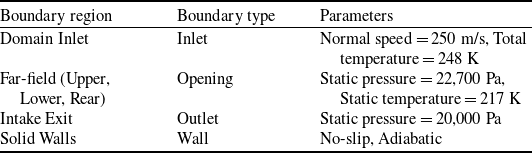

 y+


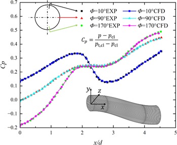


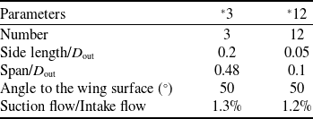

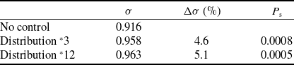

 σ


 Q=1×10⁴s−2


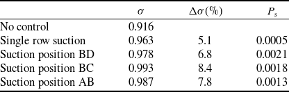

 σ


 σ


 Q=1×10⁴s−2

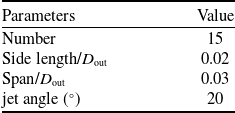


 σ
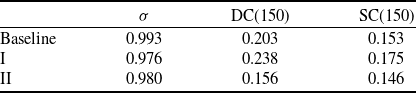




 σ