Phenotype and genotype data

Phenotypes and genotypes for sows of two purebred Landrace-origin lines (A and B) and their commercial cross (AB) were provided by Genus-Plc (Hendersonville, TN, USA).

Individual litter size (total number of piglets born per litter) records of sows genotyped were pre-corrected by fitting a linear mixed model with the lme4 (Bates et al., Reference Bates, Maechler and Bolker2012) R-package (R Core Team, 2012), to take into account the environmental random effects of number of services, mating type (natural or artificial insemination), parity order within farm, farm and month of farrow and age at first farrowing. Adjusted litter size records were obtained after subtracting the estimates of these environmental effects.

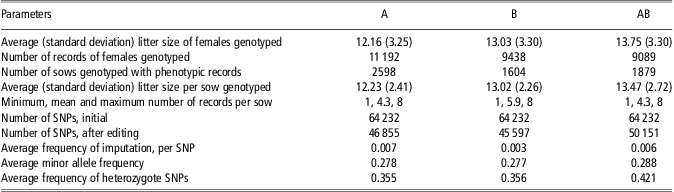
The average of adjusted litter size records per sow (PB) was the target phenotype to be predicted. Histograms of the raw litter size records, adjusted litter size records and average of adjusted litter size records are given in Supplementary Figure S1, suggesting that approximated normality holds. The number of sows with records was 2598, 1604 and 1879 in the A, B and AB lines, respectively. Sows were genotyped using the Illumina PorcineSNP60 BeadChip. SNPs with minor allele frequency <0.05 and missing genotype frequency >0.95 were removed. For the remaining loci, missing genotypes were imputed using a naïve method based on allele frequencies at each locus. Table 1 shows summary statistics of phenotypic and genotypic data for the animals in the A, B and AB lines.

Table 1

Summary statistics of phenotype and genotype data of the two purebred (A and B) and one crossbred (AB) pig lines

SNP = single-nucleotide polymorphism.

Models

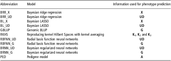
The predictive ability of six linear and five non-linear (either in the features or on the parameters) models was compared using cross-validation, with phenotypes in testing sets viewed as yet to be observed in the training sets. Comparisons were on a within line basis. A summary of these models is listed in Table 2.

Table 2

List of abbreviations for the models used

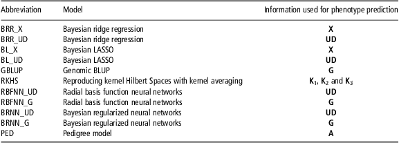
X = Matrix of marker genotypes; UD = Principal component scores of the matrix of marker genotypes; G = Genomic relationship matrix; K_i = Gaussian kernels (i = 1,2,3); A = pedigree-based numerator relationship matrix.

Linear genome-enabled models

Let y be a vector of average pre-corrected number of piglets per sow, following the linear regression model:

$$ {\bf y}\, = \,{\bf {{1}}}\mu \, + \,{\bf {{X\brbeta }}}\, + \,{\bf {{{\brepsilon}}}}$$

where $$${\bf {{y}}}\, = \,\{ {{{y}_i}\, = \,r_{i}^{{{\rm{ - 1}}}} \mathop{\sum}\nolimits_b {{{y}_{ib}}} } \},\,{{y}_{ib}}$$$ is an individual record, $$${{r}_i}$$$ is the number of records used for computing the average and b indexes an individual record; μ is an effect common to all records; $$${\bf {{\brbeta }}}\, = \,\{ {{{\beta }_j}} \}$$$ is the vector of allele substitution effects of p markers; $$${\bf {{X}}}\, = \,\{ {{{x}_{ij}}} \}$$$ is a matrix of marker covariates of dimensions n × p (j = 1,…,p and i = 1,…, n, with n being the number of phenotypes), and $$${\bf {{{\brepsilon}}}}\, = \,\left\{ {{{{\epsilon}}_i}} \right\}$$$ is the vector of residuals. In this model, the number of location parameters to be inferred largely exceeds the number of phenotypes. Hence, marker effects cannot be estimated uniquely from the likelihood function.

One approach for dealing with this issue is to use Bayesian shrinkage regression methods in which marker effects are treated as random variables. Assume that residuals follow the normal distribution, where $$$\sigma _{{\epsilon}}^{{\rm{2}}} $$$ is the residual variance of individual records. Residual correlation in the data was not accounted for in the analysis, whereas heterogeneity of residual variance was partially alleviated by weighting the residual variance by r_i (de los Campos et al., Reference de los Campos, Hickey, Pong-Wong, Daetwyler and Calus2012a). Then from equation (1), the likelihood function stems from the sampling model:

$$ p\left( {{\bf {{y}}}\left&#x007C; {{\bf {{\brbeta }}},\sigma _{{\epsilon}}^{2} } \right.} \right)\, = \,\prod _{{i\, = \,{\rm{1}}}}^{n} N({{y}_i}&#x007C;\mu \, + \,\mathop{\sum}\limits_{j\, = \,{\rm{1}}}^p {{{x}_{ij}}{{\beta }_j}}, \sigma _{{\epsilon}}^{2} /{{r}_i})$$

In the Bayesian framework prior assumptions are made about the unknown parameters, and differences in assumptions lead to different Bayesian regression models (de los Campos et al., Reference de los Campos, Hickey, Pong-Wong, Daetwyler and Calus2012a). In what follows, the two Bayesian linear regression models employed here are described.

Let all p marker effects be assigned identical and independent distributions with joint prior density $$$ p\left( {{\bf {{\brbeta }}}\left&#x007C; {\bf {{\bromega }}} \right.} \right)\, = \,\prod\nolimits_{j\, = \,{\rm{1}}}^p {p({{\beta }_j}\left&#x007C; {{\bf {{\bromega }}})} \right.} $$$ , where ω represents a collection of known parameters. Then, the posterior density of β is:

$$no{&amp; p\left( {{\bf {{\brbeta }}}\left&#x007C; {{\bf {{y}}},\sigma _{{\epsilon}}^{{\rm{2}}}, {\bf {{\bromega }}}} \right.} \right) \propto \,p\left( {{\bf {{y}}}\left&#x007C; {{\bf {{\brbeta }}},\sigma _{{\epsilon}}^{{\rm{2}}} } \right.} \right)p\left( {{\bf {{\brbeta }}}\left&#x007C; {\bf {{\bromega }}} \right.} \right)\cr &amp;\, = \,\prod _{{i\, = \,{\rm{1}}}}^{n} \,N({{y}_i}&#x007C;\mu \, + \,\mathop{\sum}\limits_{j\, = \,{\rm{1}}}^p {{{x}_{ij}}{{\beta }_j}}, \sigma _{{\epsilon}}^{{\rm{2}}} /{{r}_i})\prod _{{j\, = \,{\rm{1}}}}^{p} p({{\beta }_j}\left&#x007C; {{\bf {{\bromega }}})} \right.$$

Bayesian ridge regression (BRR) assumes that the prior density of a marker effect, $$$ p( {{{\beta }_j}\left&#x007C; {\bf {{\bromega }}} \right.} ) $$$ , is that of a Normal distribution with mean 0 and variance $$$\sigma _{\beta }^{{\rm{2}}} $$$ common to all markers, that is, $$$ p( {{{\beta }_j}&#x007C;\sigma _{\beta }^{{\rm{2}}} } \right)\, = \,N({{\beta }_j}&#x007C;0,\sigma _{\beta }^{{\rm{2}}} ) $$$ , with $$${\bf {{\bromega }}}\, = \,\sigma _{\beta }^{{\rm{2}}} $$$ . Bayesian LASSO (BL; Park and Casella, Reference Park and Casella2008), assigns a double-exponential (DE) distribution to marker effects, with mean zero and inverse scale parameter $$$\sqrt {\frac{{{{\lambda }^{\rm{2}}} }}{{\sigma _{{\epsilon}}^{{\rm{2}}} }}} $$$ , that is $$$ p( {{{\beta }_j}\left&#x007C; {\sigma _{{\epsilon}}^{{\rm{2}}} } \right.} \right)\, = \,{\rm{DE}}({{\beta }_j}\left&#x007C; 0 \right.,\frac{{{\rm{2}}\sigma _{{\epsilon}}^{{\rm{2}}} }}{{{{\lambda }^{\rm{2}}} }}) $$$ . Typically, λ ² (the square of the regularization parameter) is assigned a Gamma or a Beta distribution. The DE distribution assigns a larger mass near 0 than the Normal, but it also allows for larger marker effects because it has thicker tails. Statistically, the DE density can be represented as a mixture of scaled-normal densities, which allows structuring the original problem in terms of a hierarchical model that can be implemented via Gibbs sampling (e.g. Park and Casella, Reference Park and Casella2008; de los Campos et al., Reference de los, Naya, Gianola, Crossa, Legarra, Manfredi, Weigel and Cotes2009b).

Assuming additive allele substitution effects, SNP genotypes can be coded as –1, 0 and 1 for the homozygote for the minor allele, heterozygote and homozygote for the other allele. This leads to $$${\bf {{X}}}\, = \,\{ {{{x}_{ij}}} \} $$$ , a matrix of dimension n × p for all SNP genotypes of all individuals. For convenience, we denote BRR_X and BL_X as the Bayesian ridge regression and the Bayesian LASSO models, respectively, each using marker codes in X as the predictor variables. Aiming at reducing the number of parameters to be estimated, but without losing much of the information contained in X, we also used as covariates the principal component scores (UD) of X in our BRR and BL models. Here, UD is an n × n matrix, which is obtained from the singular value decomposition of X (Mandel, Reference Mandel1982):

$${\bf {{X}}}\, = \,{\bf {{UDV}}}&#x0027;$$

where the columns of U and V are the left and right singular vectors of X, respectively, and D is a diagonal matrix containing the non-zero-singular values of X (square roots of the non-zero eigenvalues of either XX′ or X′X). The cumulative percentage of variance explained by the components of the singular value decomposition for the three lines is shown in Figure 1. This figure illustrates the reason why we choose to keep all components of UD and not less. Since the square of the singular value is proportional to the variance explained by each singular vector, it can be seen from the histograms that each left singular vector kept in UD contributed a small amount to the variability of X.

Figure 1

Cumulative percentage of variance explained by the components of the singular value decomposition (SVD) of the marker matrix X in (a) A line, (b) B line and (c) AB line. Variance is obtained by squaring the singular values of X.

If UDV′ is used instead of X, model (1) can be re-parameterized as:

$${\bf {{y}}}\, = \,\mu {\bf {{1}}}\, + \,{\bf {{UDV}}}&#x0027;{\bf {{\brbeta }}}\, + \,{\bf {{{\brepsilon}}}}\, = \,\mu {\bf {{1}}}\, + \,{\bf {{UD}}}{{{\bf {{\brbeta }}}}^\ast} \, + \,{\bf {{{\brepsilon}}}}$$

Here, $$${{{\bf {{\brbeta }}}}^\ast} \, = \,{\bf {{V}}}&#x0027;{\bf {{\brbeta }}} $$$ , so that β* is assigned the same prior distribution as that of β in the BRR and BL models, for example, $$${{{\bf {{\brbeta }}}}^\ast} \sim N(0,{\bf {{I}}}\sigma _{{{{\beta }^\ast} }}^{{\rm{2}}} ) $$$ in ridge regression because $$${\bf {{V&#x0027;V}}}\, = \,{\bf {{I}}} $$$ . We use BRR_UD and BL_UD to represent BRR and BL models that use the UD matrix as inputs, respectively.

Intuitively, a genome-enabled best linear unbiased prediction model genomic BLUP (GBLUP) is obtained by replacing Xβ by u in model (1):

$${\bf {{y}}}\, = \,{\bf {{1}}}\mu \, + \,{\bf {{u}}}\, + \,{\bf {{{\brepsilon}}}}$$

where the residuals follow the normal distribution described previously. The vector of additive genomic effects, or genomic breeding values (GBV), $$${\bf {{u}}}\, = \,\left\{ {{{u}_i}} \right\}$$$ is assumed to be normally distributed, $$$p\left( {{\bf {{u}}}\left&#x007C; {\sigma _{u}^{{\rm{2}}} } \right.} \right)\, = \,N({\bf {{u}}}&#x007C;0,{\bf {{G}}}\sigma _{u}^{{\rm{2}}} )$$$ , where $$$\sigma _{{\rm{u}}}^{{\rm{2}}} $$$ is the additive genomic variance, and G is the genomic relationship matrix (VanRaden, Reference VanRaden2008).

$${\bf {{G}}}\, = \,\frac{{({\bf {{X}}}\,{\rm{ - }}\,{\bf {{E}}})({\bf {{X}}}\,{\rm{ - }}\,{\bf {{E}}})&#x0027;}}{{{\rm{2}}\mathop{\sum}\limits_{j\, = \,{\rm{1}}}^p {{{q}_j}(1\,{\rm{ - }}\,{{q}_j})} }}$$

Here, the G matrix can be viewed as a ‘standardized’ (co)variance matrix of genomic similarities among individuals, because genotypes in the X matrix are centered by subtracting their expected frequencies at each locus (E columns). VanRaden (Reference VanRaden2008) stated that allele frequencies at each locus q_j, for j = 1,…,p should be those of a base population under Hardy–Weinberg equilibrium, in order to avoid biased estimates of degrees of relationships and of inbreeding. However, such information was not available to us. Hence, allele frequencies were estimated from the available data. Prior distributions assigned to $$$\sigma _{\beta }^{{\rm{2}}} $$$ , $$$\sigma _{u}^{{\rm{2}}} $$$ and $$$\sigma _{{\epsilon}}^{{\rm{2}}} $$$ were proper scaled inverse χ² distributions with degrees of freedom parameter, df_l and scale parameter S_l, assigned arbitrarily so that $$$p(\sigma _{l}^{{\rm{2}}} \left&#x007C; {d{{f}_l},} \right.\,{{S}_l})\, = \,{{\chi }^{{\rm{ - 2}}}} (\sigma _{l}^{{\rm{2}}} \left&#x007C; {d{{f}_l}} \right.,{{S}_l}),\; \; {\rm{for}}\,l \in \{ \beta, u,{\epsilon}\} $$$ .

Non-linear genome-enabled models

The standard assumption made in linear methods, that is, fitting additive effects of markers only, prevents from capturing complex interactions that may exist, leading to incorrectly specified models. The use of non-parametric methods may deliver a higher predictive accuracy. In this study, three types of non-linear models were used: reproducing kernel Hilbert spaces (RKHS), Bayesian regularized neural networks (BRNN) and radial basis functions neural networks (RBFNN). RKHS is non-linear in the inputs (SNPs) but linear in the parameters; on the other hand, BRNN and RBFNN are doubly non-linear. The RKHS model was introduced in quantitative genomics by Gianola et al. (Reference Gianola, Fernando and Stella2006) and it can be represented as follows:

$${\bf {{y}}}\, = \,{\bf {{1}}}\mu \, + \,{\bf {{g}}}\, + \,{\bf {{{\brepsilon}}}}$$

where $$${\bf {{g}}}\, = \,{{\left[ {g({{{\bf {{x}}}}_1}), \ldots, g({{{\bf {{x}}}}_n})} \right]}^&#x0027;} $$$ the vector of conditional expectation functions, maps each input vector of marker information x_i of order p × 1, onto the real line. Here, the distribution of the residuals is as in model (1). The prior distribution for g is normal: $$$p({\bf {{g}}}&#x007C;\sigma _{g}^{2} )\, = \,N(0,{\bf {{K}}}\sigma _{g}^{2} )$$$ , where $$$\sigma _{g}^{{\rm{2}}} $$$ is an unknown variance and K is a n × n positive definite matrix, called the reproducing kernel matrix. K can be viewed as an expected correlation structure between pairs of points evaluated in the conditional expectation function: $$$cov({{g}_i},{{g}_{i&#x0027;}}) \propto \,K({{{\bf {{x}}}}_i},{{{\bf {{x}}}}_{i&#x0027;}})$$$ (de los Campos et al., Reference de los Campos, Gianola and Rosa2009a). Conveniently, K can be built using a Gaussian basis function: $$${\bf {{K}}}\, = \,K({{{\bf {{x}}}}_i},{{{\bf {{x}}}}_{i&#x0027;}})\, = \,\exp ({\rm{ - }}h{{\left\Vert {{{{\bf {{x}}}}_i}\,{\rm{ - }}\,{{{\bf {{x}}}}_{i&#x0027;}}} \right\Vert}^{\rm{2}}} )$$$ , where the bandwidth parameter h determines how fast the correlation between two points drops and $$$\left\Vert {{{{\bf {{x}}}}_i}\,{\rm{ - }}\,{{{\bf {{x}}}}_{i&#x0027;}}} \right\Vert$$$ is the Euclidean distance between pairs of marker genotypes. Note that the inputs (markers) enter non-linearly in K but that the RKHS model is linear in g. Prediction using RKHS methods is very sensitive with respect to values of the bandwidth parameter, making the choice of an appropriate h value important. This issue was addressed by de los Campos et al. (Reference de los Campos, Gianola and Rosa2009a), who proposed a Bayesian approach where several kernels are employed together in a model as if these represented different random factors in a linear model. Even though markers were coded for additive effects, this multi kernel approach should be capable of capturing some non-additivity (Gianola et al., Reference Gianola, Fernando and Stella2006). Following this idea, we fitted three different kernels (d = 1,2,3) each with a different h. The $$$\sigma _{{\epsilon}}^{{\rm{2}}} $$$ and the $$$\sigma _{{g,d}}^{{\rm{2}}} $$$ variances were assigned scaled inverse χ ²prior distributions.

Another type of non-linear model, both in marker covariates and parameters, that was considered for prediction was neural networks (NN). Unlike RKHS, where the basis functions used in the regression are imposed a priori, NN methods are more flexible because they are potentially capable of learning those functions from the data (González-Camacho et al., Reference González-Camacho, de los Campos, Pérez, Gianola, Cairns, Mahuku, Babu and Crossa2012). In this study, two types of single hidden layer NN were investigated: BRNN and RBFNN.

A single hidden layer feed forward NN can be seen as a two-step regression. First, information coming from the predictors or inputs (x_ij) is combined with a vector of connection strengths $$${\bf {{\brbeta }}}_{{}}^{{[t]}} \, = \,\{ {\beta _{j}^{{\left[ t \right]}} } \} $$$ at each of t hidden neurons (t = 1, 2, …, s), plus an intercept or ‘bias’ (b_t) giving the following linear score: $$$ v_{i}^{{[t]}} \, = \,{{b}_t}\, + \,\mathop{\sum}\nolimits_{j\, = \,{\rm{1}}}^p {\beta _{j}^{{\left[ t \right]}} {{x}_{ij}}} $$$ at neuron t. Each of the neuron scores is then transformed non-linearly using an activation function, $$$ z_{i}^{{[t]}} \, = \,{{g}_t}(v_{i}^{{[t]}} ) $$$ . In the output layer, the s data-derived functions are combined to yield the predicted phenotype (i.e. the output, y_i) and the model becomes:

$${{ y}_i}\, = \,\mu \, + \,\mathop{\sum}\limits_{t\, = \,{\rm{1}}}^s {{{w}_t}z_{i}^{{\left[ t \right]}} } \, + \,{{{\epsilon}}_i}$$

where w_t is the regression of the phenotype on the transformed score $$$z_{i}^{{[t]}} $$$ . The regression parameters are then $$${\bf {{\brbeta }}}\, = \,({{{\bf {{\brbeta }}}}^{[{\rm{1}}]}}, {{{\bf {{\brbeta }}}}^{[{\rm{2}}]}}, \ldots, {{{\bf {{\brbeta }}}}^{[s]}} )&#x0027;$$$ and $$${\bf {{w}}}\, = \,({{w}_{\rm{1}}},{{w}_{\rm{2}}}, \ldots, {{w}_s})&#x0027;$$$ . All neural network models used here employed the identity function in the output layer. The two variants of NN used here basically differed in the basis function used in the neurons of the hidden layer, and in the way the network was constructed and its parameters estimated. Although NN methods have a high ability of reproducing complex patterns when learning from data, they are prone to over fitting the training dataset, impeding good predictions once new data is presented to the network. This can be avoided, in part, by using regularized NN methods in which a compromise between model goodness of fit and complexity of the network is achieved (e.g. Gianola et al., Reference Gianola, Hayrettin, Weigel and Rosa2011; Okut et al., Reference Okut, Gianola, Rosa and Weigel2011).

Gianola et al. (Reference Gianola, Hayrettin, Weigel and Rosa2011) adapted the methodology for BRNN (e.g. MacKay, Reference MacKay1992) to the prediction of complex phenotypes through the use of pedigree and genomic data. The infinitesimal model and the linear regressions on markers are special cases. Let $$$\brPsi$$$ be the parameters in the neural network (connection strengths, hidden to output weights and hidden and output biases). Under a BRNN, estimates of parameters are obtained in two steps. In the first step, the posterior modes of $$$\brPsi$$$ given variance parameters $$$\sigma _{{\epsilon}}^{{\rm{2}}}, \sigma _{\psi }^{{\rm{2}}} $$$ are obtained. This is equivalent to minimizing the ‘augmented’ sum of squares, for example, Gianola et al. (Reference Gianola, Hayrettin, Weigel and Rosa2011),

$$ F({\bf {{\brPsi }}})\, = \,\eta \mathop{\sum}\limits_{i\, = \,{\rm{1}}}^n {e_{i}^{{\rm{2}}} } \, + \,\alpha \mathop{\sum}\limits_{i = {\rm{1}}}^m {\psi _{i}^{{\rm{2}}} } $$

where $$$\eta \, = \,{{(2\sigma _{e}^{2} )}^{{\rm{ - }}1}} $$$ , $$$\alpha \, = \,{{(2\sigma _{\psi }^{2} )}^{{\rm{ - }}1}} $$$ , and e_i is the model residual. Estimation of the variance components in the second step is via maximization of an approximation to the marginal likelihood of the data, $$$p({\bf {{y}}}\left&#x007C; {\sigma _{{\epsilon}}^{{\rm{2}}} } \right.,\sigma _{\psi }^{{\rm{2}}} )$$$ , a procedure known as empirical Bayes. Steps one and two are iterated until convergence.

RBFNN (Broomhead and Lowe, Reference Broomhead and Lowe1988) is another NN method that uses a Gaussian radial basis function in the hidden neurons:

$$ z_{i}^{{[t]}} \, = \,exp\left[ {{\rm{ - }}\,{{h}_t}\,{{{\left\Vert {{{{\bf {{x}}}}_i}\,{\rm{ - }}\,{{{\bf {{c}}}}_t}} \right\Vert}}^{\rm{2}}} } \right]$$

The function is defined by the Euclidean norm between the input vector x_i of the individual and a centroid vector c_t. Here, h_t is a bandwidth parameter that needs to be determined empirically. An algorithm was used to select orthogonal centroids sequentially in order to decrease the mean square error between the observed response and the predicted output (Chen et al., Reference Chen, Cowan and Grant1991). Number of centroids, that is, the number of neurons, grows up to a certain desired precision or up to the number of inputs. To make computations feasible, we used as inputs to the networks either the additive genomic relationship matrix (BRNN_G and RBFNN_G models, for Bayesian regularized neural networks and radial basis functions neural networks, respectively) or principal component scores of the SNP matrix (BRNN_UD and RBFNN_UD models, for Bayesian regularized neural networks and radial basis functions neural networks, respectively).

Pedigree-based linear model

As a benchmark, we also assessed the predictive ability of a pedigree-based linear mixed-effects model (PED), as follows:

$${\bf {{y}}}\, = \,{\bf {{1}}}\mu \, + \,{\bf {{a}}}\, + \,{\bf {{{\brepsilon}}}}$$

where a is the vector of additive genetic effects which, according to the standard assumptions of the infinitesimal model, is assumed to be normally distributed as: $$$N({\bf {{a}}}&#x007C;0,{\bf {{A}}}\sigma _{a}^{{\rm{2}}} )$$$ , where $$$\sigma _{a}^{{\rm{2}}} $$$ is the additive genetic variance and A is the numerator additive genetic relationship matrix among individuals, obtained from the pedigree. Residuals were normally distributed, as described previously. The prior distributions for $$$\sigma _{a}^{{\rm{2}}} $$$ and $$$\sigma _{{\epsilon}}^{{\rm{2}}} $$$ were scaled inverse χ ² distributions, each with 4 degrees of freedom and a scale parameter equal to 1.

Markov chain Monte Carlo (MCMC) implementation and software used

Hyper-parameters df_l and S_l of the scaled inverse χ ² distribution of $$$\sigma _{l}^{{\rm{2}}} $$$ , for $$$l \in \{ \beta, u,{\epsilon}\} $$$ , were set to 4 and 1 in each of the BRR, BL and GBLUP models; this gives a prior density with a prior expectation of one half of the sample variance of the standardized phenotypes (González-Camacho et al., Reference González-Camacho, de los Campos, Pérez, Gianola, Cairns, Mahuku, Babu and Crossa2012). The rate and shape parameters of the prior gamma distribution in the BL models were set to 1 × 10⁻⁴ and 0.6, respectively. More details regarding specifications, guidelines for choosing hyper-parameters and computational implementation of these models can be found in de los Campos et al. (Reference de los, Naya, Gianola, Crossa, Legarra, Manfredi, Weigel and Cotes2009b) and Pérez et al. (Reference de los, Naya, Gianola, Crossa, Legarra, Manfredi, Weigel and Cotes2010). The degrees of freedom and scale parameters of the scaled inverse χ ² distributions of $$$\sigma _{{\epsilon}}^{{\rm{2}}} $$$ and the $$$\sigma _{g}^{{\rm{2}}} $$$ of the RKHS models, were set to 5 and to half the variance of the phenotypes, respectively. The R-package (R Core Team, 2012) BLR (de los Campos and Pérez, Reference de los Campos and Pérez2012) was used to implement BRR and BL. All RKHS models and the PED model were implemented using a script provided by de los Campos et al. (Reference de los Campos, Gianola, Guilherme, Kent and Crossa2010). Briefly, single chains of 100 000 iterations were run, with the first 50 000 iterations discarded as burn-in. Samples drawn from the posterior distributions of the parameters of interest were saved every 100 rounds and then used for statistical inference, with means used as point estimates. The network architecture used in the BRNN models was a single hidden layer with four neurons, with the activation functions being hyperbolic-tangent. Models were run using a C++ program (written by the authors and available upon request) but an R-package (R Core Team, 2012) version is also available (BRNN; Pérez et al. Reference Pérez-Rodríguez, Gianola, Weigel, Rosa and Crossa2013). Radial basis functions NN models were implemented using the newrb neural network function from the MATLAB Neural Network Toolbox™ [MATLAB 7.11.0.584 (R2010b), The MathWorks Inc., Natick, MA, USA, 2000]. For each of the RBFNN, the median of the Euclidean distance between each pair of vectors of the input matrix (i.e. elements of G or from the UD) was the value used as bandwidth. A sum-squared error of 0.02 was the precision goal assigned for stopping the algorithm.

Assessment of predictive ability of yet to be observed phenotypes

A 10-fold cross-validation was used to test the predictive performance of these models within each of the lines A, B and AB. For each line, the dataset was randomly split into approximately 10 equal parts. Marker effects and the overall mean were estimated based on a collection of nine portions (90%) of the data, referred to as training set, and predictive ability was assessed in the remaining (10%), used as testing set. Such a training–testing cycle was repeated ten times in total by rotating the 10 portions for training and testing, with each portion used for testing only once and for training nine times. Predictive ability of each model for each dataset was evaluated via Pearson's correlation (r) between observed and predicted phenotypes in testing sets.

Predictive ability across models

The three panels in Figure 2 show the average correlations between observed and predicted litter size phenotypes in the testing sets from the 10-fold CV in lines A, B and AB, respectively. In general, the ability of predicting litter size was low (r ranged from 0.15 to 0.23 with a standard deviation across the 10-folds that ranged from 0.05 to 0.11 across models). This could be because of the low heritability and repeatability of litter size. Heritability estimates for average litter size obtained with the PED model were 0.21, 0.14 and 0.19 for A, B and AB lines, respectively. Reliabilities of genome-based predictions of fertility traits in dairy cattle have been lower than those obtained for more heritable traits, such as milk production and composition (Hayes et al., Reference Hayes, Bowman, Chamberlain, Verbyla and Goddard2009). Nevertheless, several authors have argued that genome-based prediction could be of special interest for increasing rate of genetic gain for lowly heritable traits if a sufficiently large number of records per individual is available for training the models (Ibañez-Escriche and Gonzalez-Recio, Reference Ibañez-Escriche and Gonzalez-Recio2011). If one assumes a repeatability of 0.15 for litter size, the correlation between one record or the average of three records of an individual and a future record (Falconer and MacKay, Reference Falconer and MacKay1996) is expected to range between 0.15 and 0.35, respectively. Hence, our correlations were similar to those expected from a repeatability model with only one or two records available for prediction of future litter size. However, genomic information allows obtaining predictions much earlier in life than when using phenotypic data only. Selection decisions for litter size are made before a progeny record is available, so a model with predictive ability equivalent to that from a record of one progeny represents significant cost-savings to the industry.

Figure 2

Average correlations between observed and predicted litter size phenotypes obtained from a 10-fold cross-validation for (a) A line (b) B line and (c) AB line. See Table 2 for model abbreviation.

Although genomic selection (GS) has been already applied in dairy cattle breeding programs, research on benefits for other species are scarce (Ibañez-Escriche and Gonzalez-Recio, Reference Ibañez-Escriche and Gonzalez-Recio2011). Lillehammer et al. (Reference Lillehammer, Meuwissen and Sonesson2011) reported that use of genomic information in pig breeding could improve genetic gain by reducing generation interval, increasing selection accuracy, and reducing inbreeding rate, when compared with conventional selection without progeny testing. Furthermore, there is early evidence from commercial data that pig breeding can benefit from GS as well. For example, Cleveland et al. (Reference Cleveland, Forni, Garrick and Deeb2010), using de-regressed EBVs as phenotypes, reported accuracies of GEBV of 0.65 and 0.50 for total number born and stillborn, respectively, which are similar to those reported in dairy cattle (VanRaden et al., Reference VanRaden, Van Tassell, Wiggans, Sonstegard, Schnabel, Taylor and Schenkel2009).

Predictive ability of genome-based linear models

The five linear genome-enabled prediction models showed small differences in predicting future litter size in the three datasets. On average, the correlation ranged from 0.20 to 0.23 (Figure 2). Within the linear models, BRR_UD had the lowest predictive performance in each of the three lines. In general, predictive ability was not affected much by type of shrinkage (i.e. prior distribution on substitution effects) or by type of genomic information (individual markers v. principal component scores).

Predictive ability of genome-based non-linear models

RKHS performed similarly to the linear models and, on average, the correlation was ∼0.23 in all three datasets. RKHS can be implemented easily using standard mixed model packages (de los Campos et al., Reference de los Campos, Gianola and Rosa2009a; Piepho, Reference Piepho2009), and it is computationally efficient because it has n + 1 unknowns only, which is typically much smaller than the p unknowns in marker-based BRR or BL. Use of RKHS maybe of special interest in crossbred populations, because dominance can be represented in an additional kernel, in which case there would be an additional n unknowns, as opposed to 2p effects in a model with additive and dominance effects of each of the SNPs. It has been shown that RKHS can outperform linear models in predictive ability in chickens (González-Recio et al., Reference González-Recio, Gianola, Long, Weigel, Rosa and Avendaño2008) and plants (Crossa et al., Reference Crossa, de los Campos, Pérez, Gianola, Burgueño, Araus, Makumbi, Singh, Dreisigacker, Yan, Arief, Banziger and Braun2010; González-Camacho et al., Reference González-Camacho, de los Campos, Pérez, Gianola, Cairns, Mahuku, Babu and Crossa2012). Heslot et al. (Reference Heslot, Yang, Sorrells and Jannink2012) compared the predictive performance of different linear and non-linear GS models for several traits in plants and found that, overall, linear and non-linear models performed similarly. RKHS seemingly gave the best predictive ability: for example, in 16 out of their 18 comparisons RKHS outperformed Bayes Cπ (Habier et al., Reference Habier, Fernando, Kizilkaya and Garrick2011).

The two neural network models gave mixed results. On average, the correlation ranged from 0.16 to 0.23 for RBFNN and BRNN. The predictive ability of BRNN varied drastically in the three lines. They delivered the worst predictions in A but were best in AB. The BRNN_UD and BRNN_G yielded the best predictive ability in the crossbred dataset, where non-additive genetic effects such as dominance are to be expected. Using different network architectures, Gianola et al. (Reference Gianola, Hayrettin, Weigel and Rosa2011) found that BRNN outperformed a linear model when predicting yield traits in dairy cows (Gianola et al., Reference Gianola, Hayrettin, Weigel and Rosa2011). By reducing the number of markers from all the SNPs available, Okut et al. (Reference Okut, Gianola, Rosa and Weigel2011), also found that BRNN could produce a predictive performance similar to linear regression models using mouse data. Pérez-Rodríguez et al. (Reference Pérez-Rodríguez, Gianola, González-Camacho, Crossa, Manès and Dreisigacker2012), evaluating a wheat population also found that the predictive ability of BRNN was similar to that of the BL and other linear models. These results suggest that NN models, which are flexible non-linear systems, may predict complex phenotypes better than linear models. Unfortunately our study with litter size could not corroborate this unambiguously, because of the large cross-validation uncertainty. Presumably use of dominance code inputs could enhance the prediction ability of BRNN and RKHS models even further. We found that the predictive abilities of the RBFNN models were higher when using UD than when using G as inputs to the network. González-Camacho et al. (Reference González-Camacho, de los Campos, Pérez, Gianola, Cairns, Mahuku, Babu and Crossa2012) assessed the predictive performance of BL, RKHS and RBFNN in simulated data and in several trait-environment combinations of maize datasets. They found similar predictive ability among different models, but RKHS and RBFNN performed more consistently across traits than BL. Our results indicate that NN have the potential of outperforming other linear and non-linear GS models when predicting litter size under certain conditions, but care must be taken to avoid overfitting. Semi-parametric genomic prediction methods can deliver a better predictive performance than the linear methods provided that kernels, network architecture and inputs are carefully selected (Gianola et al., Reference Gianola, Fernando and Stella2006).

Predictive ability by type of genomic information used

A model can be viewed as providing a direct GS approach if the genomic estimated breeding values (GEBV) are estimated directly, as the PED model does in a single step, or as an indirect GS approach if individual marker effects are estimated first, and then the GEBV are computed as the sum of marker effects (times genotype codes) for each individual. For example, GBLUP and RKHS are direct GS approaches, and BRR and BL are indirect. Several simulation studies have shown that the predictive ability may differ between these two types of approaches, depending on marker coverage of the genome and, perhaps, the genetic architecture of the target trait (de los Campos et al. Reference de los Campos, Hickey, Pong-Wong, Daetwyler and Calus2012a). However, some models that can be formulated in both manners, such as GBLUP and Ridge regression BLUP should not show differences in prediction ability. In our data, different GS models had similar predictive ability. Likewise, Maltecca et al. (Reference Maltecca, Parker and Cassady2012) did not found marked advantages of several direct GS models (BL, Bayes A and semi-parametric methods) over GBLUP in Holstein data. An advantage of direct GS methods is that they deal conveniently with the p >> n issue because the large number of SNP genotypes is used only for computing a (co)variance matrix of genomic kinships among individuals, of dimension n × n, before model fitting. In GBLUP, the G matrix was obtained here following VanRaden (Reference VanRaden2008), with kinships among individuals based on additive similarities at each locus. In RKHS, Euclidean norms between pairs of vectors of marker genotypes are used to compute kernels. Both types of relationships, that is, G and the kernel matrices, were constructed under the assumption that all SNPs had the same contribution toward explaining the degree of relatedness among individuals. This could create a possible ‘dilution effect’ of those that truly contribute to signal. For instance, alleles with a low allelic frequency that are present in a pair of individuals may be more informative of kinship than if the two individuals share common alleles.

A better predictive ability from using principal component scores instead of all original marker scores may be because of dimensionality reduction and elimination of redundancy of explanatory variables. However, we did not observe improvement in predictive ability when using principal component-based genomic models. Actually, the predictive ability was lower when principal component scores were used as explanatory variables in BRR (−3.4% on average), but this difference was smaller in BL. Use of the UD matrix as an input led to improved predictive ability (∼4% on average) in the RBFNN models, relative to what was observed when the G matrix was the input. Perhaps principal component scores are more informative as an input than the G matrix. However, this was not corroborated with the other type of NN used, since BRNN_G obtained the best predictive results in the B and AB lines and the worst in A. We did not construct a cross-validation distribution, so it may be that these differences are because of chance.

In most cases, the predictive ability of a genome-based model was higher than that from PED. This was probably because of the fact that realized relationships among individuals are captured by marker information. This is in agreement with previous findings (see e.g. de los Campos et al., Reference de los Campos, Hickey, Pong-Wong, Daetwyler and Calus2012a). For example, predictive accuracy using various types of genomic relationship matrices was higher than when using a pedigree-based kinship matrix in pigs (Forni et al., Reference Forni, Aguilar, Misztal and Deeb2010). Likewise, reliabilities for predicting daughter yield deviations of several traits for Holstein bulls were higher when genomic information was used than when only parent averages were employed (VanRaden et al., Reference VanRaden, Van Tassell, Wiggans, Sonstegard, Schnabel, Taylor and Schenkel2009). Our results are consistent with these observations, that is, predictive accuracy can be increased if genomic information is used for predicting the phenotypes of candidates.

Predictive ability in the different lines

The average correlation between observed and predicted phenotypes in testing sets from all models was higher in the crossbred (0.26) than in the purebred lines (0.15 and 0.22, for A and B lines, respectively). Posterior mean estimates of the additive genetic variance obtained with PED were 0.94, 0.50 and 1.02 for A, B and AB lines, respectively suggesting that the amount of genetic variance in crossbreds was larger. Within purebred lines, predictive ability for the B population was higher than in A, although the B line had fewer animals (1604 v. 2598 sows) and heritability was slightly lower than in A (0.21 and 0.14 for A and B lines, respectively). These differences in predictive ability may be because of differences between lines in effective sample size, or perhaps are related to hidden population structure. Summary statistics for the three datasets are given in Table 1. Raw average litter size per sow was slightly larger in the AB line. This is probably a consequence of inbreeding depression recovery, capture of heterosis and complementarity effects (Falconer and MacKay, Reference Falconer and MacKay1996) on reproductive performance. The average number of records per sow varied from 2.26 in the B line to 2.72 in the AB line. Average minor allele frequency was similar for the three lines. Sows from the AB line had a higher level of heterozygosity (7% more) than in purebred lines. This is also reflected by the size of diagonal elements of the G matrices of the three lines (Figure 3a). The magnitudes of the diagonal entries of G increase with the number of loci that are homozygote in an individual, and these elements were larger in the A and B lines than in AB. Possibly, selection for improvement of maternal traits may have may have caused fixation of favorable alleles at loci in chromosome regions in strong linkage disequilibrium with causal variants (Falconer and MacKay, Reference Falconer and MacKay1996). This would also contribute toward an increased degree of inbreeding in the purebred lines, which dissipates in their cross as it can be noticed in the magnitudes of the diagonal entries of A (Figure 3b).

Figure 3

Boxplots of the diagonal elements of (a) the genomic relationship matrices (G) and (b) the additive genetic kinship matrix obtained from the pedigree (A) for the two purebred (A and B) and the crossbred lines (AB).

Histograms of the off-diagonal elements of the G matrices (Figure 4a–c) indicated that these were larger and more variable in purebred lines than in AB, and the distribution was bimodal in B and skewed in A. Predictive ability should be better if individuals in training and testing have more molecular similarity or genetic relatedness (de los Campos et al., Reference de los Campos, Vazquez, Klimentidis and Sorensen2012b). However, if genomic similarity among individuals is high in a population, this reduces effective population size, accordingly (Falconer and MacKay, Reference Falconer and MacKay1996). If this is the case, a large sample size may be required for obtaining reliable predictions, impairing predictive ability within purebreds relative to what would be observed in crossbred lines. The bimodal or skewed distribution of off-diagonal elements of G in the purebred lines may be suggesting hidden population structure in these lines. Histograms of the off-diagonal elements of the A matrices (Figure 4d–f) were markedly bimodal. Although being more similar in their genome, the degree of relatedness among purebred individuals was lower than in the crossbreds. This could have also contributed to a weaker degree of genetic connectedness between training and testing sets in purebred lines, thus impairing predictive ability.

Figure 4

Histograms of the off-diagonal elements (values) of the (a to c) genomic relationship matrices (G) and (d to f) the additive genetic kinship matrix obtained from the pedigree (A) for the two purebred (A and B) and the crossbred (AB) lines.

We examined this issue further by plotting the first two principal components of G and A (Figure 5). Plots of the two first principal components of G showed the presence of clusters only in the A and B lines, but not in line AB. Within purebreds, clustering was more noticeable in A (where the worst predictions were attained) than in B. These clusters indicate that molecular similarity in sows of purebred lines was not homogeneous over individuals, probably resulting from family aggregation, given that clusters were also observed for the purebred lines in the plots of the 2 first principal components of the additive genetic kinship matrix obtained from the pedigree. This also suggests that a cross-validation distribution from random partitions into training and testing datasets may be misleading, as one would expect that predictive ability is larger within than between clusters (Habier et al., Reference Habier, Tetens, Seefried, Lichtner and Thaller2010). The level of linkage disequilibrium (LD) between markers and QTLs impacts prediction accuracy, and this is impaired if individuals in training and testing are not genetically related (de los Campos et al., Reference de los Campos, Vazquez, Klimentidis and Sorensen2012b). Random partitioning assumes that individuals are homogeneous with respect to genetic relationships, family structure, demography and linkage disequilibrium relationships (Cleveland et al., Reference Cleveland, Forni, Garrick and Deeb2010). In our study, the same 10-fold CV was used for assessing performance of all models, so hidden structure is not expected to influence the comparison among models. However, ignoring population structure may have hampered predictive ability in purebred lines relative to what was observed in the AB line. It would be of interest to develop strategies for improving predictive ability in purebred lines by properly accounting for population structure. Daetwyler et al. (Reference Daetwyler, Kemper, van der Werf and Hayes2012) stated that a large part of prediction accuracy was because of population structure, with LD between markers and QTL playing a smaller role. Methods for accounting for population structure in prediction were investigated by Janss et al. (Reference Janss, de los Campos, Sheehan and Sorensen2012).

Figure 5

Plots of the first two principal components (1st and 2nd PC) of (a to c) the genomic relationship (G) and (d to f) the additive genetic kinship matrix obtained from the pedigree (A) for the purebred (A and B) and crossbred (AB) lines.