1 Introduction
Cloud cavitation remains a significant area of research in hydrodynamic flows, where, due to its violent unsteady nature, it may cause lift reduction, vibration, noise and erosion. The mechanisms involved in cavity formation, detachment and condensation, or collapse, of shed clouds are not yet fully understood. These may involve several phenomena including free and surface nucleation, surface energy effects and cavity interfacial instabilities, cavity/boundary layer interaction, laminar to turbulent transition, large-scale turbulence, re-entrant jet formation and shockwave formation.
Interest in these phenomena has spanned more than half a century. With advances in both computational and experimental capabilities, more recent investigations have provided valuable insight into the underlying physics. Examples include Stutz & Reboud (Reference Stutz and Reboud1997, Reference Stutz and Reboud2000) and Coutier-Delgosha et al. (Reference Coutier-Delgosha, Stutz, Vabre and Legoupil2007) which provide detailed measurements on the internal flow and structures within the cavity, including the presence of a re-entrant flow. In particular, the work by Callenaere et al. (Reference Callenaere, Franc, Michel and Riondet2001) reported that large-scale instability and cavity shedding phenomena are shown to be associated with re-entrant jet formation.
The general phenomena of shockwaves in bubbly flows are now well understood, as reviewed and described by Brennen (Reference Brennen2005). However, substantial progress into the analysis of shock/acoustic phenomena in larger-scale cavitating structures has only been made in the last two decades with, in particular, the combined numerical and experimental work undertaken by Brennen and co-workers through the 1990s (Reisman, Wang & Brennen Reference Reisman, Wang and Brennen1998). Several groups have been developing X-ray imaging as a diagnostic tool for cavitating flows. Studies involving both internal converging–diverging type geometries and lifting-surface bodies are of current interest (see respectively Khlifa et al. (Reference Khlifa, Coutier-Delgosha, Fuzier and Roussette2016), Ganesh, Mäkiharju & Ceccio (Reference Ganesh, Mäkiharju and Ceccio2016a ) and Ganesh, Wu & Ceccio (Reference Ganesh, Wu and Ceccio2016b )). Concurrently, numerical methods are being developed, capable of analysing these complex unsteady flows, to complement these new experimental results (Gnanaskandan & Mahesh Reference Gnanaskandan and Mahesh2016a ). Ganesh et al. (Reference Ganesh, Mäkiharju and Ceccio2016a ) used time-resolved X-ray densitometry to investigate large-scale shedding mechanisms of cavitation forming on the apex of an asymmetric triangular prism within a rectangular duct flow. They showed that large-scale shedding may be due to re-entrant jet formation but also condensation shockwave propagation. From direct measurement of the cavity Mach number, they showed that, should this reach a threshold value, shockwaves may form, causing an additional mechanism for large-scale shedding. Ganesh et al. (Reference Ganesh, Mäkiharju and Ceccio2016a ) also provide a recent extensive review of the field of cloud cavitation.
Kawakami, Qin & Arndt (Reference Kawakami, Qin and Arndt2005) reported on cloud cavitation about a hydrofoil, where shedding resulted in periods of fully wetted flow and re-nucleation, such that nucleation may influence cloud formation. Brandner et al. (Reference Brandner, Walker, Niekamp and Anderson2010) made similar observations for cloud cavitation about a sphere, where shedding resulted in cycles of cavity extinction and re-nucleation over large circumferential regions. Guennoun (Reference Guennoun2006) showed that cavitation inception about a hydrofoil may be due to surface nucleation as well as free nucleation, and how this is dependent on surface topographical and chemical properties. The role of the boundary layer and interactions with nucleated bubbles, and their development into attached cavities, also formed part of this work. The influence of nucleation and initial cavity development on cloud cavitation, however, remains largely to be investigated.
While cloud cavitation about lifting surfaces is of particular interest, it also occurs about bluff bodies, although the latter case is little reported on, as was shown in the review by Brandner et al. (Reference Brandner, Walker, Niekamp and Anderson2010). A recent contribution by Gnanaskandan & Mahesh (Reference Gnanaskandan and Mahesh2016b ) has illustrated the present state of the art in the numerical modelling of these complex dynamic multiphase flows, although, being two-dimensional cylinder flows, they are not directly comparable to the present work.
Cloud cavitation about a sphere is of interest as a canonical flow for both computational and experimental investigation. Such bodies of revolution may be tested in a water tunnel free from direct wall effects and have sufficient volume for inclusion of instrumentation. The present study builds on earlier work by Brandner et al. (Reference Brandner, Walker, Niekamp and Anderson2010) on cloud cavitation about a sphere, involving several experimental improvements that enable greater insight. Experiments were performed in a water tunnel in which the dissolved gas and free bubble populations could be strictly controlled. Through tailoring of surface and water properties, inception could be restricted to either free or surface nucleation. For the present work, the test water was maintained depleted of microbubbles, such that any free nuclei were of sufficient strength not to be activated in the test flow. The model sphere was manufactured to provide a continuous consistent surface of known properties over the region of inception and leading edge detachment. Simultaneous surface pressure measurement and high-speed imaging were used to gain further insights into the shedding physics and to derive high-resolution power spectrograms of the shedding frequencies as a function of the cavitation number.
2 Experimental overview
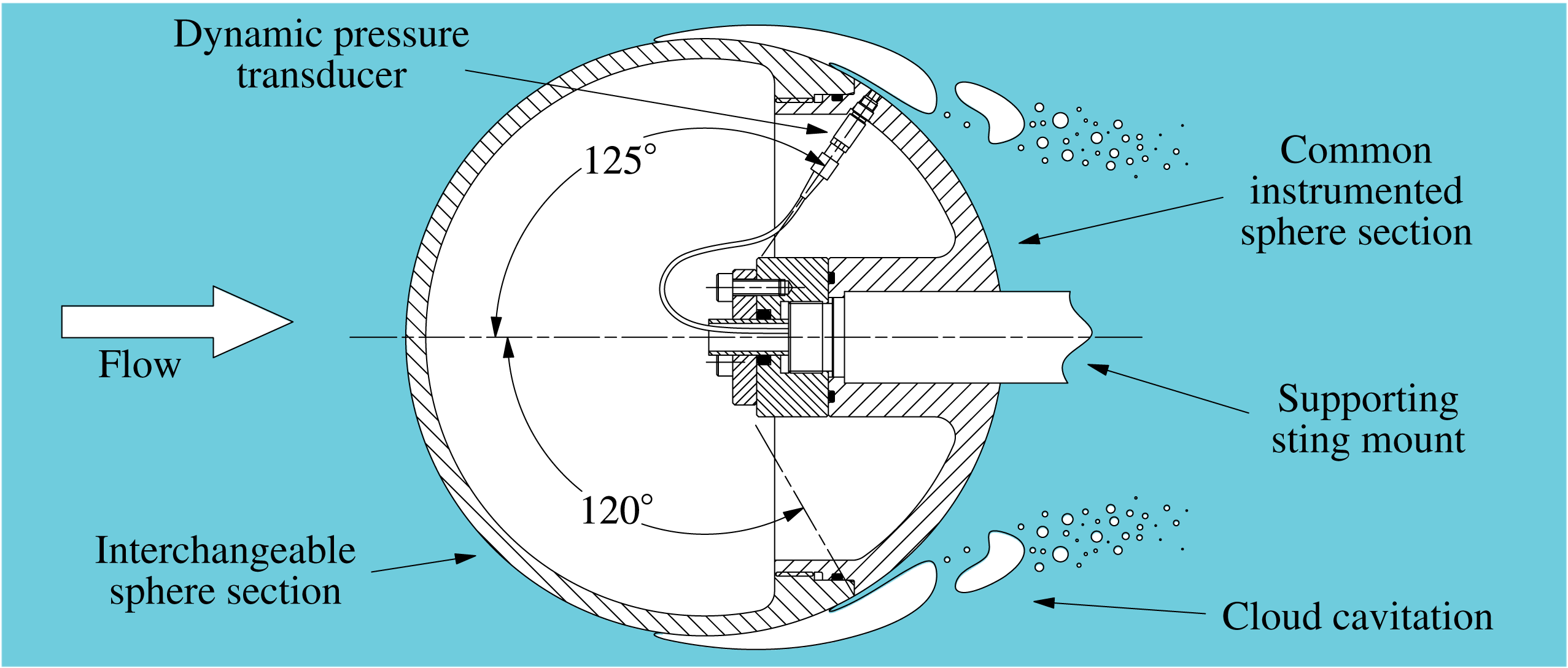
A 0.15 m diameter sphere was sting-mounted on the centreline of the variable-pressure water tunnel at the Cavitation Research Laboratory at the Australian Maritime College, University of Tasmania. The tunnel has a test section of 0.6 m square
 $\times$
2.6 m long, in which the pressure can be varied in the range 4–400 kPa and the velocity in the range 2–
 $12~\text{m}~\text{s}^{-1}$
. The sphere had a polyvinyl chloride (PVC) front section, extending
 $120^{\circ }$
from front stagnation, as shown in figure 1. A 3 mm diameter flush-mounted dynamic pressure sensor (PCB 105C02) was located within the stainless steel rear section
 $125^{\circ }$
from front stagnation. The sensor was located to be within the cavitation shedding zone. Data were recorded from the pressure sensor for 2 s at 7000 Hz using a National Instruments PXIe-4497 card. High-speed photography was recorded simultaneously with the pressure measurements using a LaVision HighSpeedStar8 camera with a Nikkor 50 mm f/1.8 lens, with illumination provided by two LED lamps. The sphere was oriented to have the pressure sensor in the camera field of view on the sphere horizontal centreline. Additional longer data series from the pressure sensor alone were recorded at 1024 Hz for 200 s. High-resolution images were captured using a Canon EOS 50D camera with a 24–70 mm f/2.8 lens illuminated with triggered stroboscopic lighting (DRELLO 1018/LE4040).
Pressure measurements and high-speed photography were recorded at a Reynolds number of
 $1.5\times 10^{6}$
and cavitation numbers ranging from 1.0 to 0.375 in 0.025 increments. The Reynolds number is defined as
 $Re=UD/\unicode[STIX]{x1D708}$
, where
 $D$
is the sphere diameter,
 $U$
is the test section velocity and
 $\unicode[STIX]{x1D708}$
is the kinematic viscosity of the water. The cavitation number is defined as
 $\unicode[STIX]{x1D70E}=2(p-p_{v})/\unicode[STIX]{x1D70C}U^{2}$
, where
 $p$
is the static pressure at the test section centreline,
 $p_{v}$
is the vapour pressure and
 $\unicode[STIX]{x1D70C}$
is the water density. The dissolved oxygen content of the water was maintained at 3.3 ppm. The susceptibility of the water, or strength of the natural or free nuclei, under these conditions was measured using a cavitation susceptibility meter (CSM), giving critical pressures of approximately
 $-100$
kPa (equivalent to bubbles of the order of
 $1\unicode[STIX]{x03BC}\text{m}$
diameter) at concentrations of
 $0.1~\text{cm}^{-3}$
. The operating principle of the CSM involves passing water continuously sampled from the tunnel through a venturi, with a centre body, to develop a controlled underpressure in the venturi throat. All viable nuclei with critical pressures greater than the throat pressure are activated and counted. The venturi geometry was that given by Pham, Michel & Lecoffre (Reference Pham, Michel and Lecoffre1997). No artificial nuclei were injected.
Schematic of the sphere experimental set-up, showing the PVC front section and stainless steel rear section. The 0.15 m diameter sphere is mounted from a 0.023 m diameter sting on the test section centreline. The PVC front section extends
 $120^{\circ }$
from front stagnation. The rear section has a flush-mounted dynamic pressure sensor located within the shedding zone (
 $125^{\circ }$
from front stagnation).

3 Results
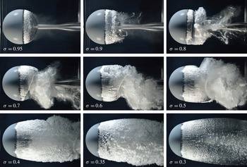
A set of still images depicting the development of cloud cavitation about the sphere with reduction in
 $\unicode[STIX]{x1D70E}$
from just below inception through to supercavitation is shown in figure 2. Excerpts from the high-speed photography at
 $\unicode[STIX]{x1D70E}$
values from 1.0 to 0.4 in 0.1 increments are available online at https://doi.org/10.1017/jfm.2016.819 (movies 1–7). Inception occurs at approximately
 $\unicode[STIX]{x1D70E}=1.0$
(not shown), where intermittent cavitation occurs around the circumference of minimum pressure. The minimum pressure coefficient,
 $C_{p\,min}=2(p_{min}-p)/\unicode[STIX]{x1D70C}U^{2}$
, is approximately
 $-1.0$
for a transcritical or supercritical sphere (Achenbach Reference Achenbach1972), implying
 $p_{min}\approx p_{v}$
, which is much greater than the measured critical pressure (approximately
 $-100$
kPa) of the free nuclei noted above. For the minimum pressure to reach the critical pressure of the free nuclei, for the present test conditions,
 $\unicode[STIX]{x1D70E}$
would need to be reduced to approximately
 $-1.0$
. This suggests that inception and re-nucleation associated with shedding are likely to be due to surface nucleation.
At
 $\unicode[STIX]{x1D70E}=0.95$
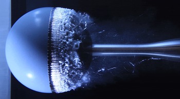
, a circumferential cavity is fully established, with the leading edge of the cavity composed of periodic laminar cells, as shown in figure 3 (for
 $\unicode[STIX]{x1D70E}=0.9$
). The overlying laminar flow in the separating boundary layer transitions to turbulence with the formation of transverse waves due to Kelvin–Helmholtz (K–H) instability. Brandner et al. (Reference Brandner, Walker, Niekamp and Anderson2010) show that the properties of these waves for the same conditions compare closely with those for free laminar shear layers and laminar boundary layers at cavity detachment from bluff objects, providing strong evidence that they are due to inviscid instability. As part of the present work, wavelength measurements were made for spheres of differing geometric scale for the same cavitation and Reynolds numbers, showing these waves to scale precisely with the physical scale or equivalently with the boundary layer thickness, providing further support that they are due to K–H instability in the overlying shear layer. In figure 3, evidence of these waves can be seen on the cavity surface. Cavity breakup at high
 $\unicode[STIX]{x1D70E}$
values, where cavity lengths are small, is due to the development of these transverse waves, which with intermittent roll-up are shed as coherent axisymmetric vortices.
High-resolution images depicting cavitation development about the sphere at
 $Re=1.5\times 10^{6}$
for
 $\unicode[STIX]{x1D70E}$
values ranging from just below inception through to supercavitation.

A photograph of cavity development at
 $\unicode[STIX]{x1D70E}=0.9$
, showing the leading edge to be composed of periodic laminar cells. The separated overlying boundary layer transitions to turbulence with the formation of transverse waves due to Kelvin–Helmholtz instability which with intermittent roll-up are shed as coherent axisymmetric vortices.

As
 $\unicode[STIX]{x1D70E}$
is reduced below 0.9 and cavity lengths increase, re-entrant jets form due to the strong adverse pressure gradient about the sphere. Re-entrant flow develops with initial cavity formation, accumulating with growth, to ultimately contact or impinge upon the growing cavity surface. This impingement initiates cavity breakup, from which condensation shockwaves propagate in every case, causing further cavity breakup. From the high-speed photography, it is not possible to discern the precise mechanism of shockwave initiation, but that they propagate from the region of re-entrant flow impingement in every shedding cycle. When the shedding is most energetic, upstream shockwave propagation may cause leading edge extinction, after which the cavity re-nucleates. Cavity lengths increase with
 $\unicode[STIX]{x1D70E}$
reduction, and the re-entrant jet forms further downstream, becoming detached from the sphere body at approximately
 $\unicode[STIX]{x1D70E}=0.675$
. As the cavity continues to increase in length, shedding events occur less often. For
 $\unicode[STIX]{x1D70E}<0.3$
, the cavity enters the supercavitating regime. The physics of these shedding regimes is described in greater detail below together with quantitative measurements.
3.1 Large-scale shedding mechanisms and correlation with surface pressure
Analysis of the high-speed photography and surface pressure measurements shows that large-scale shedding commences with reduction of
 $\unicode[STIX]{x1D70E}$
below approximately 0.9. At these
 $\unicode[STIX]{x1D70E}$
values, cavity lengths become sufficient (approximately
 $0.25D$
) for re-entrant jet flow to develop. As the cavity lengths are less than the sphere diameter, the shedding is near axisymmetric, as may be seen in figure 2. It was observed that for
 $\unicode[STIX]{x1D70E}<0.9$
, re-entrant jet flow always formed with each shedding cycle, the accumulation of which led to cavity impingement at approximately mid-length. In every case, a shockwave propagated from this region of impingement, condensing at least part or the full length of the cavity, causing leading edge extinction over large regions of the circumference. In the case of leading edge extinction, re-nucleation would rapidly follow, with the cavity growing anew. The delay to re-nucleation and cavity re-growth reduced with decreasing
 $\unicode[STIX]{x1D70E}$
, such that at low
 $\unicode[STIX]{x1D70E}$
values, approaching supercavitation, re-nucleation and re-growth were apparently instantaneous. As the cavity forms downstream of the sphere minimum pressure, the formation of re-entrant jet flow and its accumulation may be attributed to the large adverse pressure gradient acting over the closure region. As
 $\unicode[STIX]{x1D70E}$
is reduced and cavity lengths increase, the larger-scale re-entrant flows on opposing sides of the sphere begin to interact, creating instability and asymmetry in the shedding. This asymmetry leads to frequent occurrences of converging re-entrant flows, creating local jetting from which the shockwave can be seen to propagate both upstream and circumferentially (online movie 5).
This mechanism of shockwave initiation about a bluff body is in contrast to that observed for the flows reported by Ganesh et al. (Reference Ganesh, Mäkiharju and Ceccio2016a ), where shockwaves form probabilistically with Mach number increase beyond a critical value. This result may be attributable to the significant differences between these flows. As noted above, the strong adverse pressure gradient about the sphere always results in re-entrant fluid impinging upon the cavity surface, which does not occur in the flows with milder adverse pressure gradients investigated by Ganesh et al.
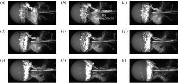
High-speed photographic sequence of part of a shedding cycle for
 $\unicode[STIX]{x1D70E}=0.75$
(every 10th image from a 7000 Hz recording). The re-entrant jet forms as the cavity grows (a), and initially impinges on the cavity surface locally (b), and then more generally (c). A shockwave propagates upstream (d), condensing the cavity (e). The cavity leading edge is reduced to a line of small bubbles (f), followed by complete extinction (g–h) over a portion of the visible circumference before re-nucleating and growing anew (i). This sequence is available in online movie 8.

A sequence of images from the high-speed photography of part of a typical shedding cycle at
 $\unicode[STIX]{x1D70E}=0.75$
is shown in figure 4, and a corresponding excerpt is available online (online movie 8). The sequence is of every 10th image from the photography recorded at 7000 Hz (1.429 ms intervals). The growing axisymmetric cavity (a) has a defined trailing edge, showing the development of the re-entrant jet flow. The jet fluid may be seen to initially contact the cavity surface locally (b) and then more generally along the visible circumference (c). A shockwave propagates upstream from the affected circumferential region, condensing the cavity (d), leaving only spanwise cavitating vortical filaments (e). These small-scale filaments are advected downstream and roll up with the large-scale shed cloud (f). The upstream shockwave propagation initially reduces the cavity to a peripheral line of small bubbles (f) which is apparently then fully condensed over a portion of the circumference (g–h). The new cavity then develops from re-nucleation or remnant small-scale cavities left after the shockwave passage (i).
The occurrence of shockwaves for every shedding cycle (large-scale shedding regime) suggests that the Mach number is consistently greater than a threshold, as described by Ganesh et al. (Reference Ganesh, Mäkiharju and Ceccio2016a
). The shock wave propagation speeds have been estimated from space–time plots extracted from a single horizontal row of pixels (on the sphere centreline) from the high-speed imaging. These were found to vary from cycle to cycle about a constant mean value of approximately
 $-1.1U$
for all cavitation numbers. These values are somewhat higher but similar to the values measured by Ganesh et al. for lower cavitation numbers generating free streamline flows with higher upstream void fractions. This is consistent with the case of flow about the sphere, where free streamline flows occur for all large-scale shedding.
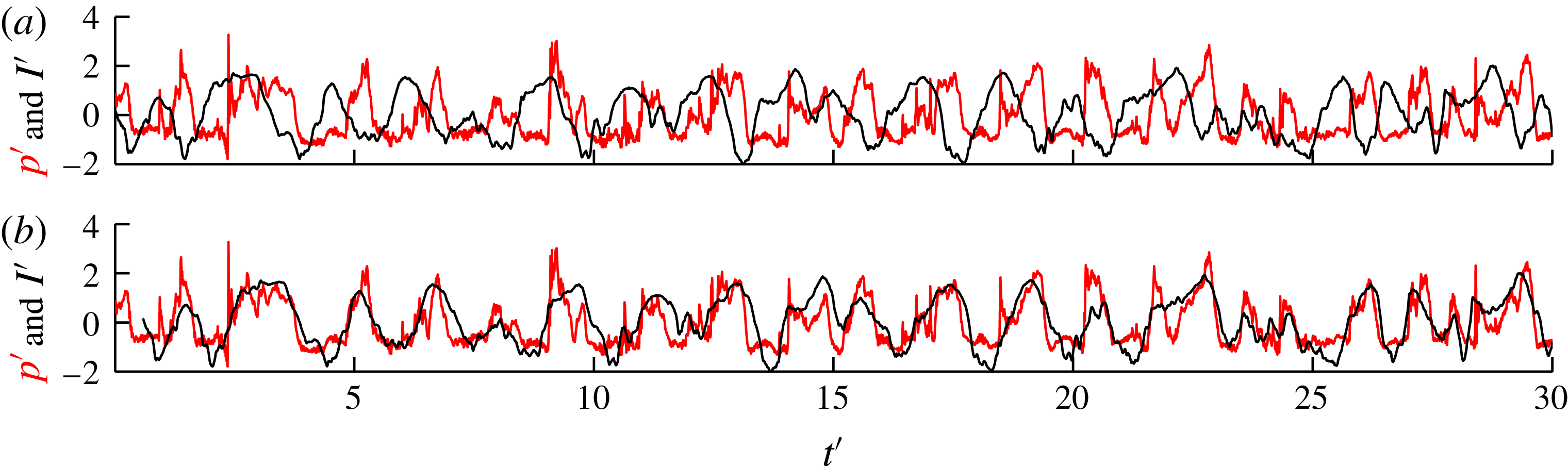
Time series of average light intensity over a
 $65\times 65$
pixel window, centred over the surface pressure sensor location, have been extracted from the high-speed photography for comparison with surface pressure measurements. The size of the sampled window was determined to minimise noise while providing the required spatial resolution. The time series were, however, found to be relatively insensitive to window size (de Graaf, Brandner & Pearce Reference de Graaf, Brandner and Pearce2014). An example of the simultaneously recorded intensity and surface pressure signals for
 $\unicode[STIX]{x1D70E}=0.8$
is shown in figure 5(a). Both signals have been normalised by subtracting the mean and dividing by the standard deviation, giving the normalised intensity,
 $I^{\prime }$
, and the normalised pressure,
 $p^{\prime }$
. Time,
 $t$
, has been non-dimensionalised by
 $t^{\prime }=Ut/D$
. The intensity signal has been inverted so that a low average pixel intensity (i.e. clear water) corresponds to a high pressure and a high average pixel intensity (i.e. white vapour cloud) corresponds to a low pressure. The phase difference between the two signals, with
 $I^{\prime }$
leading
 $p^{\prime }$
, may be attributed to the temporal variation between the streamwise position of the cavity and the pressure magnitude at the sensor due to the cycles of alternating re-entrant flow and vapour cavity growth. As the cavity grows over the sensor, the re-entrant flow induces a pressure maximum just prior to the intensity value reaching its maximum. As the coupled re-entrant jet and shockwave separate the cavity to form a shed cloud, the surface pressure returns to a minimum, after which the intensity also returns to a minimum with the passing of the cloud. The delay between the signals can be found using cross-correlation, and in this case is 8.3 ms (or
 $t^{\prime }=0.57$
). Figure 5(b) shows the two signals aligned with
 $I^{\prime }$
shifted by
 $t^{\prime }=0.57$
to become
 $I_{s}^{\prime }$
. Across the range of
 $\unicode[STIX]{x1D70E}$
studied, the delay varies from 8.1 to 11.0 ms (
 $t^{\prime }=0.56{-}0.77$
). For
 $0.9>\unicode[STIX]{x1D70E}>0.4$
, where shedding is most active, Pearson’s correlation coefficient for
 $p^{\prime }$
–
 $I_{s}^{\prime }$
time series was found to vary between approximately 0.6 and 0.8.
Simultaneously acquired time series of normalised surface pressure and light intensity at the surface pressure sensor location for
 $\unicode[STIX]{x1D70E}=0.75$
(a). The phase difference between the two signals is due to the temporal variation between the streamwise position of the cavity and the pressure magnitude. The intensity time series may be shifted,
 $I_{s}^{\prime }$
, (b) by the temporal difference from cross-correlation of 8.3 ms (or
 $t^{\prime }=0.57$
) to give improved correlation.

3.2 Spectral content and coherence
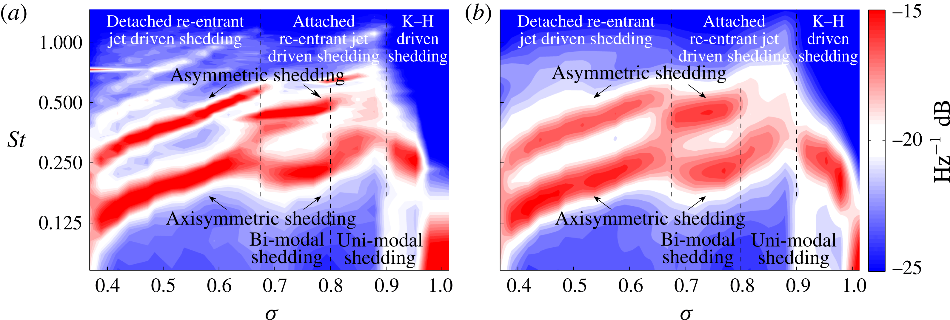
The power spectral densities of the long sampled normalised pressure signals were analysed using the Welch (Reference Welch1967) and wavelet (Torrence & Compo Reference Torrence and Compo1998) methods. Power spectrograms were obtained for
 $\unicode[STIX]{x1D70E}$
values ranging from 1.0 to 0.375 in 0.025 increments, as shown in figure 6. For the Welch method, these were derived using a Hamming window length of 1024 and 50 % overlap. The power spectrogram for the same data using a Morlet-6 wavelet is derived using a smallest wavelet scale of
 $2~\text{d}t$
and a scale spacing of 0.25, where
 $\text{d}t=1/1024~\text{s}$
is the sample period. The frequencies,
 $f$
, are non-dimensionalised as Strouhal numbers,
 $St=fD/U$
. Both plots show similar overall structure, with the Welch power spectrogram showing more defined peaks. The variation of root-mean-square pressure,
 $C_{p\,RMS}=2_{p\,RMS}/\unicode[STIX]{x1D70C}U^{2}$
, with
 $\unicode[STIX]{x1D70E}$
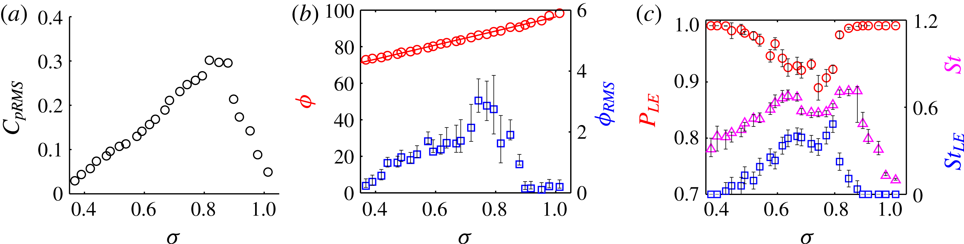
is shown in figure 8(a).
Power spectrograms of cavity shedding Strouhal number as a function of
 $\unicode[STIX]{x1D70E}$
for values ranging between inception (
 $\unicode[STIX]{x1D70E}\approx 1.0$
) and approaching supercavitation (
 $\unicode[STIX]{x1D70E}<0.3$
) in increments of
 $0.025\unicode[STIX]{x1D70E}$
. Spectra derived using the Welch method (a) and the Morlet-6 wavelet method (b). Three distinct shedding regimes are evident: one where shedding is uni-modal and two where it is bi-modal.

Three distinct regimes are evident in figure 6. For
 $\unicode[STIX]{x1D70E}>0.9$
, shedding is uni-modal at initially low
 $St$
values, increasing as
 $\unicode[STIX]{x1D70E}$
is reduced from 1.0 (inception) to 0.9. As noted in § 3.1, for this range of
 $\unicode[STIX]{x1D70E}$
values where cavity lengths are small, breakup is due to fine-scale K–H waves forming in the overlying separated laminar boundary layer (as shown in figure 3). With the development of these waves, the cavity trailing edge is broken up into small-scale cavitating vortices which with intermittent roll-up are shed as coherent axisymmetric vortices. As
 $\unicode[STIX]{x1D70E}$
is reduced and cavity lengths increase, greater vapour volumes are shed, increasing the frequency of the larger-scale shedding. The value of
 $C_{p\,RMS}$
increases in a linear trend with
 $\unicode[STIX]{x1D70E}$
reduction in this regime, as shown in figure 8(a).
As
 $\unicode[STIX]{x1D70E}$
is reduced below 0.9, cavity lengths increase sufficiently for re-entrant flow and large-scale shedding to develop. As discussed in § 3.1 for
 $\unicode[STIX]{x1D70E}<0.9$
, shedding is driven by coupled re-entrant jet and shockwave formation. This change in regime is also reflected in
 $C_{p\,RMS}$
, where a step increase occurs between
 $\unicode[STIX]{x1D70E}$
of 0.9 and 0.875, as shown in figure 8(a). Shedding in this regime is initially uni-modal (
 $0.9>\unicode[STIX]{x1D70E}>0.8$
), where cavity lengths are small and clouds are shed close to axisymmetrically. As
 $\unicode[STIX]{x1D70E}$
is reduced, cavity lengths increase downstream of the sphere and re-entrant flows either side of the sphere begin to interact, creating instability and asymmetric shedding. The high-speed and high-resolution photography show that the cavity circumferential length variation is generally limited to one wavelength, corresponding to axisymmetric or asymmetric modes. For
 $\unicode[STIX]{x1D70E}<0.8$
, bi-modal shedding ensues, corresponding to axisymmetric (lower frequency band) and asymmetric (upper frequency band) modes, as shown in figure 6.
Ganesh et al. (Reference Ganesh, Wu and Ceccio2016b ) observed for shedding about a hydrofoil that growing cavities may be affected by pressure pulses from the collapse of previously shed cavities. They also observed that with reduction of the cavitation number, shedding transitions from uni-modal to multi-modal simultaneous with the onset of shockwaves. These results are in contrast to the present work, where shockwaves, due to the re-entrant jet mechanism described above, are present for both uni-modal and bi-modal regimes. For the sphere also, no evidence of coupling between previously shed and growing cavities was apparent in the uni-modal regime. This would imply that for the sphere the strong adverse pressure gradients and consequent re-entrant flow dominate over other potential effects that may occur for flows with milder adverse gradients. The high-speed imaging and extracted space–time plots show collapse of shed clouds, although no influence of these was evident on growing cavities, or that this affected the mode or spectral content of the shedding.
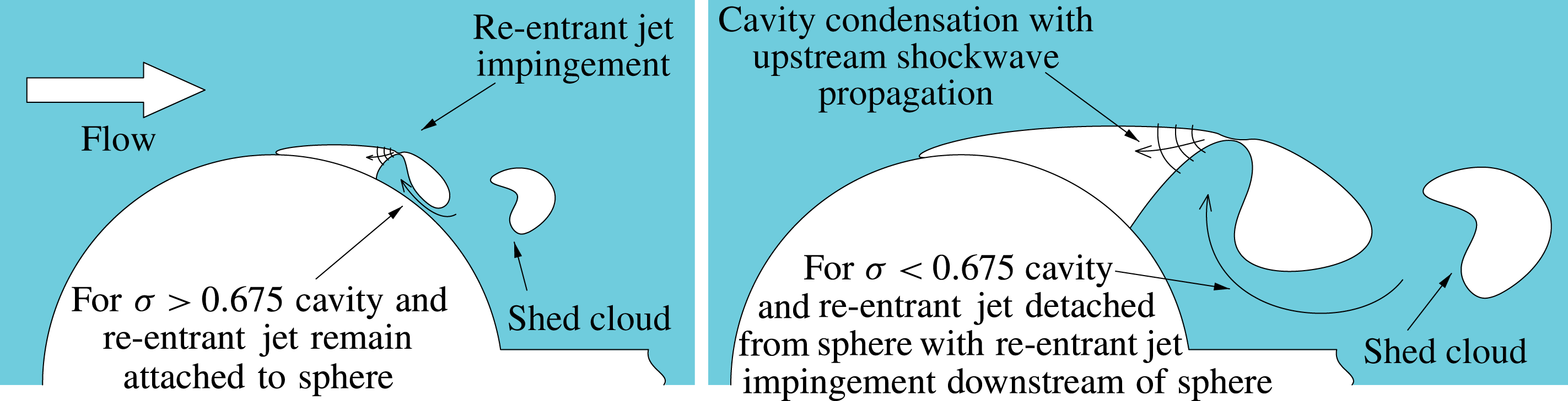
Schematic depiction of the cavity and re-entrant behaviour for the two large-scale shedding regimes in which bi-modal shedding occurs. In the first regime, for
 $\unicode[STIX]{x1D70E}>0.675$
, the cavity and re-entrant jet remain attached to the sphere, whereas in the second regime, for
 $\unicode[STIX]{x1D70E}<0.675$
, the combined cavity and re-entrant jet flow is detached from the sphere, with jet impingement occurring downstream of the sphere.

Both modes reduce in frequency with decreasing
 $\unicode[STIX]{x1D70E}$
(cavity length increase) until
 $\unicode[STIX]{x1D70E}\approx 0.675$
, where a frequency increase and discontinuity occurs in both modes despite increasing cavity lengths. The high-speed and high-resolution photography show that for
 $\unicode[STIX]{x1D70E}>0.675$
the growing cavity and re-entrant jet remain attached to the sphere, whereas for
 $\unicode[STIX]{x1D70E}<0.675$
the growing cavity is detached from the sphere and the re-entrant jet impinges upon the cavity downstream of the sphere, thereby no longer interacting with the sphere. This change is depicted schematically in figure 7. A comparison of typical asymmetric shedding events from the high-speed imaging at
 $\unicode[STIX]{x1D70E}=0.625$
and 0.7 shows both to have growth and collapse periods of approximately 19 and 11 ms respectively, or total periods of approximately 30 ms, corresponding to
 $St\approx 0.5$
. Cavity lengths at re-entrant jet impingement are approximately
 $0.70D$
and
 $0.60D$
for
 $\unicode[STIX]{x1D70E}=0.625$
and 0.7, giving cavity growth rates of 5.8 and
 $5.1~\text{m}~\text{s}^{-1}$
respectively. That is, the increase in cavity growth rates provides a sudden frequency increase despite the greater cavity length. The Welch derived power spectrogram in figure 6(a) shows an apparent overlap on the higher-frequency asymmetric mode, suggesting that either regime may occur at the transition depending on the cavity length. The location change of re-entrant jet impingement can be observed in the high-speed photography provided online, particularly online movie 4 (
 $\unicode[STIX]{x1D70E}=0.7$
), where the cavity and re-entrant jet remain attached to the sphere, and online movie 5 (
 $\unicode[STIX]{x1D70E}=0.6$
), where the cavity is detached and the re-entrant jet may be seen to impinge downstream of the sphere. Within this third regime, shedding frequencies decrease logarithmically with decreasing
 $\unicode[STIX]{x1D70E}$
, until supercavitation develops for
 $\unicode[STIX]{x1D70E}<0.3$
. The magnitude of
 $C_{p\,RMS}$
reduces linearly with decreasing
 $\unicode[STIX]{x1D70E}$
, as shown in figure 8(a), over both large-scale shedding regimes.
The variation of root-mean-square pressure,
 $C_{p\,RMS}$
, (a), the mean,
 $\unicode[STIX]{x1D719}$
, and root-mean-square,
 $\unicode[STIX]{x1D719}_{RMS}$
, of the cavity leading edge angular position measured from front stagnation (b) and the probability of leading edge presence,
 $P_{LE}$
, the leading edge extinction frequency,
 $St_{LE}$
, and the cavity shedding frequency,
 $St$
, (c).

3.3 Leading edge dynamics and statistics
Parameters describing cavity leading edge spatial and temporal behaviour as a function of
 $\unicode[STIX]{x1D70E}$
, derived from the high-speed photography, are presented in figure 8. These include the mean,
 $\unicode[STIX]{x1D719}$
, and root-mean-square,
 $\unicode[STIX]{x1D719}_{RMS}$
, of the cavity leading edge angular position measured from front stagnation, the leading edge extinction frequency,
 $St_{LE}$
, and the probability of leading edge presence,
 $P_{LE}$
. These data were derived from a sampled window 23 spanwise pixels by
 $\pm 40$
streamwise pixels either side of the leading edge mean detachment location. The presence of a leading edge is defined as an edge detection for at least one of the 23 spanwise pixels. A leading edge shedding event is counted for the first frame where no leading edge is found, if that frame is more than 100 frames from the last event, to prevent erroneous events from being counted during cavity re-establishment. The cavity shedding frequency,
 $St$
, derived from event counting, is also shown for comparison with
 $St_{LE}$
.
The variation of
 $\unicode[STIX]{x1D719}$
with
 $\unicode[STIX]{x1D70E}$
is apparently unaffected by changes in the shedding regime, reducing linearly from approximately
 $98^{\circ }$
at inception (
 $\unicode[STIX]{x1D70E}=1.0$
) to approximately
 $73^{\circ }$
approaching supercavitation (
 $\unicode[STIX]{x1D70E}=0.375$
). For
 $\unicode[STIX]{x1D70E}>0.9$
, where shedding is driven by small-scale features, the leading edge is stable and
 $\unicode[STIX]{x1D719}_{RMS}$
remains relatively small. With the onset of large-scale shedding for
 $\unicode[STIX]{x1D70E}<0.9$
,
 $\unicode[STIX]{x1D719}_{RMS}$
suddenly increases, with maximum values measured for
 $\unicode[STIX]{x1D70E}$
values ranging between 0.8 and 0.75. These maxima correspond to the onset of bi-modal shedding in the attached flow shedding regime (figure 6). This is in contrast to the maximum
 $C_{p\,RMS}$
values that occur for
 $\unicode[STIX]{x1D70E}$
values corresponding to the onset of uni-modal attached large-scale shedding. With further reduction of
 $\unicode[STIX]{x1D70E}$
,
 $\unicode[STIX]{x1D719}_{RMS}$
gradually decreases, reducing to pre-large-scale shedding values approaching supercavitation. As with
 $\unicode[STIX]{x1D719}$
, the variation of
 $C_{p\,RMS}$
with
 $\unicode[STIX]{x1D70E}$
shows no apparent changes that correspond with the changes in large-scale shedding regimes.
Cavity leading edge extinction only occurs for large-scale shedding due to shockwave formation, as measured by
 $St_{LE}$
and
 $P_{LE}$
. The general variation of
 $St_{LE}$
with
 $\unicode[STIX]{x1D70E}$
corresponds to that of
 $St$
, with the greatest ratio
 $St_{LE}/St$
occurring at
 $\unicode[STIX]{x1D70E}=0.8$
. The frequency
 $St_{LE}$
has two maxima at
 $\unicode[STIX]{x1D70E}$
values of approximately 0.8 and 0.675. Both maxima occur for bi-modal shedding. The first corresponds to the onset of bi-modal shedding in the attached flow regime and the second to the change between attached and detached regimes. With reduction of
 $\unicode[STIX]{x1D70E}$
beyond the second peak,
 $St_{LE}$
gradually reduces with increasing cavity speed and length. For
 $\unicode[STIX]{x1D70E}<0.45$
, condensation shockwaves and cavity shedding events do occur, but do not result in large-scale extinction of the leading edge, and/or the leading edge is re-nucleated so quickly that few extinction events are counted. Similar behaviour is reflected in the variation of
 $P_{LE}$
with
 $\unicode[STIX]{x1D70E}$
, although only a general minimum at approximately
 $\unicode[STIX]{x1D70E}=0.75$
occurs. The lack of correspondence of extreme values between the variation of
 $St_{LE}$
and
 $P_{LE}$
implies variations in the duration of extinction events with
 $\unicode[STIX]{x1D70E}$
or with shedding regime.
4 Conclusions
The spectral content and shedding mechanisms of cavitation about a sphere at a Reynolds number of
 $1.5\times 10^{6}$
were investigated using high-speed photography and unsteady surface pressure measurements. The variation and phase of surface pressure with the cycle of cavity growth, re-entrant jet formation and detachment were established from simultaneous high-speed photography and surface pressure measurement. Power spectrograms of surface pressure showed three shedding regimes depending on the cavitation number, ranging between inception (
 ${\approx}1$
) and supercavitation (
 ${\approx}0.3$
). These include a uni-modal regime at high cavitation numbers and two bi-modal regimes at lower cavitation numbers. At high cavitation numbers (
 ${>}0.9$
), where cavity lengths are small, breakup is driven by small-scale instabilities in the overlying boundary layer. At cavitation numbers below 0.9, greater cavity lengths allow large-scale shedding to develop driven by coupled re-entrant jet formation and shockwave propagation. Strong adverse pressure gradients about the sphere lead to accumulation and radial growth of re-entrant flow, initiating breakup from which in every case a condensation shockwave propagates, causing cavity collapse upstream. The bi-modal response is due to cavity shedding being either axisymmetric or asymmetric, with cavity circumferential length variation limited essentially to one wavelength. At intermediate cavitation numbers, where shedding is most energetic, shockwave propagation upstream causes cavity leading edge extinction, the extent of which depends on the shedding mode. The two bi-modal regimes correspond to cavitation numbers where the cavity and re-entrant jet remain attached or become detached from the sphere. This transition occurs at a cavitation number of approximately 0.675 and results in a distinct frequency offset between the two regimes in both shedding modes. The second bi-modal regime initially exhibits shorter shedding periods due to increased cavity growth rates that occur with cavity detachment. The shedding modes observed about the sphere are in contrast to those observed for flows with milder adverse gradients (Ganesh et al.
Reference Ganesh, Mäkiharju and Ceccio2016a
,Reference Ganesh, Wu and Ceccio
b
). No coupling between shed and growing cavities was observed. Changes in spectral content and shedding modes were associated with cavity length and flow symmetry rather than with the occurrence of shockwaves. Shockwaves were observed to occur in all large-scale modes, predominantly upstream for axisymmetric modes and both upstream and circumferentially in asymmetric modes.
Acknowledgements
The authors wish to acknowledge the support of the University of Tasmania and the Australian Defence Science and Technology Group. Wavelet software was developed by C. Torrence and G. Compo and was obtained at http://paos.colorado.edu/research/wavelets/.
Supplementary movies
Supplementary movies are available at https://doi.org/10.1017/jfm.2016.819.