1. INTRODUCTION
A single GPS receiver using only pseudoranges in C/A code is able to determine user position to an accuracy in the order of magnitude of 10 m; this depends on a number of error and noise sources that affect the system. The main factors responsible for accuracy reduction are: errors due to signal propagation through the ionosphere and troposphere, satellite ephemeris error, satellite and receiver clock synchronization errors and multipaths. These errors can be partially or completely removed using special techniques such as Differential GPS (DGPS, Kaplan and Hegarty, Reference Elliot and Christopher1996) based on using two receivers simultaneously. Thanks to the use of DGPS techniques it is possible to increase the accuracy of results provided by the standard GPS system in order to use them for special applications such as seismic surveillance (the Land Survey and cartography, “1994 Federal Radionavigation Plan”, 1995) and in the aerospace field because it can provide the level of accuracy required for aircraft instrument landing or, using two receivers, to determine the aircraft or LEO (Low Earth Orbit) satellite attitude.
There are different types of DGPS such as the Local Area DGPS (LADGPS) and the Wide Area DGPS (WADGPS), (Kaplan and Hegarty, Reference Elliot and Christopher1996), where a geo-referenced receiver calculates its position and compares it with the real position, in such a way that it can calculate the corrections which are transmitted to receivers in the surrounding area; finally there is a further type of DGPS which uses a mathematical approach for the reduction of the errors referred to as “Carrier phase tracking” based on interferometric relations between receivers and satellites, (Kaplan and Hegarty, Reference Elliot and Christopher1996). This method makes it possible to achieve a significant increase in accuracy combining the two sets of measurements available at the receivers: pseudorange and carrier phase measurements.
Many efforts have been devoted to searching for an algorithm able to solve the carrier-cycle ambiguities. That most frequently used is the LAMBDA method (Misra and Per Enge, Reference Patrap and Per2006), (Jonge and Tiberius, Reference Paul and Christian1996), (Teunissen et al. Reference Teunissen, De Jonge and Tiberius1996) and (Chang and Yang, Reference Chang, Yang and Zhou2005); this method solves the problem of determining carrier-cycle ambiguities but it is applicable only in post-processing analysis of data, because its convergence time is quite long. Other algorithms for carrier-cycle ambiguity resolution, such as the Wide Lane technique (Wolfe et al., Reference Jonathan, Jason and Soonsik2007), use simultaneously the dual frequency nature of the GPS signal structure. Using this technique, the process to determine the combination of carrier phase ambiguities is faster, but the requirements for a receiver able to receive both frequencies are very stringent; moreover the use of this technique is subject to errors due to the noise of the system which becomes six times greater (Kaplan and Hegarty, Reference Elliot and Christopher1996).
The new method proposed is inspired by the LAMBDA method, as formulated by Van Graas and Braasch (Kaplan and Hegarty, Reference Elliot and Christopher1996), (Graas and Braasch, Reference Van Graas, Braasch and Winter1992). This method for identifying carrier phase ambiguities was proposed, developed and tested and it shows both a short convergence time and highly accurate results even on data achieved with one moving receiver; moreover it does not require the use of dual frequencies.
In the second section of the paper the standard algorithm implemented and used for the determination of the relative position of two receivers using the Filtered Double Differences (FDD) is analysed. These FDDs are provided by the Kalman filter as a result of the combination of pseudoranges and carrier phase DDs. In the same chapter the results achieved for collected data are discussed, analyzing the influence on the position accuracy obtained using different combinations of satellites with different values of GDOP (Geometry Dilution Of Precision). This analysis was required in order to obtain the minimum optimum set of satellites to be used for receiver position determination. The number of the satellites used for DGPS should be kept low to guarantee brief calculation time.
In the third section the newly developed algorithm is explained and tested on the resolution of carrier phase ambiguity of data collected during static or moving receivers applications.
2. RESOLUTION OF BASELINE VECTOR USING FILTERED DDs
2.1. Double difference filtering method
This algorithm determines the baseline vector between the two receivers using the results provided by a standard Kalman filter. The algorithm reduces noise that characterizes the pseudorange DDs by using the carrier phase DDs; in particular, the filter predicts the values of smoothed DDs merging the inaccurate but unambiguous DDs derived from pseudoranges with the extremely accurate but ambiguous carrier phase DDs.
The application to collected data is based on DDs evaluated every second. The temporary unavailability of the satellites, resulting in data fragmentation, is estimated by using linear interpolation. The minimum combination of satellites to be used to calculate receiver positions through the Kalman filter is selected on the basis of the DOP indexes (Dilution Of Precision), (Kaplan and Hegarty, Reference Elliot and Christopher1996). The DOP indexes are calculated on the basis of the satellite position achieved by ephemeris and of the reference receiver position provided by the receiver itself. This makes it possible to choose the four independent DDs obtained by the combination of satellites with the lowest mean DOP index.
Once the DDs to be used have been chosen the Kalman filter is applied to evaluate the baseline vector (b); the algorithm used is well known but is given to complete the information in Appendix 1.
2.2. Filtering method application
The Kalman filter was applied to measurements collected at the same time by two static receivers to evaluate the effects of the GDOP on the random walk of the rover receiver positioning. This made it possible to establish a method to determine the minimum set of satellites to be used in the differential GPS application.
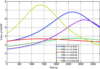
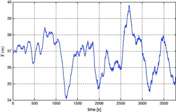
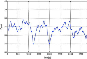
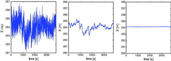
Figure 1 shows the values of the GDOP indexes obtained from the analysis of data obtained during the static acquisition. Sketched data refers to the six satellites simultaneously in view of both receivers during the whole experiment grouped by five as requested for the minimum set adaptation to evaluate DDs. The optimal set of satellites is given by PRN 1, 11, 19, 22 and 28 while the worst is given by PRN 11, 14, 19, 22 and 28. The resulting x coordinate of the baseline vector, evaluated in both cases, is sketched in Figures 2 and 3 as an example. The module of the standard deviation of the baseline vector length calculated by the satellite set with the worst GDOP is 1·92 m while that obtained from the satellite set with the best GDOP is 1·08 m.
Comparisons between GDOP indexes obtained from different combinations of satellites.

X coordinate of the baseline vector determined using the satellites set with the worst GDOP value.

X coordinate of the baseline vector determined using the satellites set with the best GDOP value.

It is evident that using the smoothed code provides better accuracy than a single GPS receiver can provide. Nevertheless these measurements are still affected by pseudorange noises, thus, to obtain more accurate positioning, it is necessary to solve the carrier phase ambiguity.
3. CARRIER PHASE AMBIGUITY RESOLUTION ALGORITHM AND ITS APPLICATION
3.1. Description and implementation of the algorithm for carrier phase ambiguity resolution
The way to increase the precision and accuracy of results provided by the DGPS system is to solve the carrier phase ambiguity. The algorithm used to determine the baseline vector (b) through ambiguity resolution is a second step, based on the results achieved by the smoothed code. The new algorithm is identical to the previous up to DDs filtering. The substantial difference is in the different use of the filtered DDs that, contrary to what happened before, are not used directly in the calculation of b, but are used to determine the carrier phase ambiguity. Once integer ambiguities are determined they are added to the carrier phase DDs which are used for the determination of b instead of filtered DDs.
The method for solving carrier phase ambiguity can be described by comparing, first of all, the expressions of the carrier phase and pseudorange DD (1 and 2):


where:
• p and q are the two satellites emitting the GPS signal,
• k and m are the two receiver antennas,
• DD km,cppq and DD km,prpq are respectively the carrier phase and pseudorange DDs,
• ɸkmpq is a combination of the fractional phase measured by the two receivers k and m with respect to satellites p and q,
• N kmpq is the integer number of wavelengths including the ambiguity,
• S kmpq are the noises affecting the carrier phase measurement,
• t kmpq is the time of flight DD evaluated considering both receivers k and m and the satellites p and q,
• Q kmpq are noises affecting the pseudoranges,
• c is the speed of light.
Multiplying equation (1) by the wavelength of the L1 (λ) it is possible to convert the DD km,cppq into metres:

It is possible to assume that the filtered DDs have the same structure as pseudorange DDs, but the error (R) in this case is much smaller than the error achieved by pseudorange DDs. The filtered DDs (pointed out only as DD S) are:

Theoretically the carrier phase DDs converted to metres should be identical in value to the filtered DDs without the errors that characterize them except for the ambiguity. So comparing t (3) and (4) it is possible to achieve:

Now substituting (5) into (3), it is possible to calculate an initial estimate of ambiguity based on carrier phase and smoothed DDs as follows:
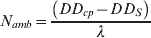
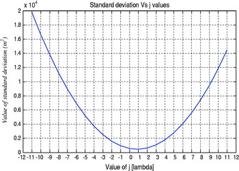
The estimate of integer ambiguity obtained is not yet reliable because it is affected by the oscillations of filtered DDs due to the low accuracy of the pseudoranges. To overcome this problem, a preliminary ambiguity guess value (GV) is achieved by choosing the mean value given applying (6) to a short acquisition (two minutes in example). Starting from this first estimate of the ambiguity and keeping in mind that the error on the smoothed code, as reported in literature (Kaplan and Hegarty) is about 2 m (±11λ), it can be stated that the real solution will be included in the range between DD cp+GV−11⋅λ and DD cp+GV+11⋅λ. Any of 23 cases included in this interval are analysed in a time interval longer than the interval used to achieve the GV.
The final ambiguity value is obtained applying the least squares technique to the deviations between smoothed and calculated DDs. In mathematical terms, the value of searched ambiguity is achieved by minimizing expression (7).

where:
• n is the length of the definition interval,
• DD cp are the carrier phase DDs,
• DD s are the smoothed DDs,
• N(j) is the value of the integer ambiguity estimated using the formula (6) with −11<j<+11 added where j∊Z.
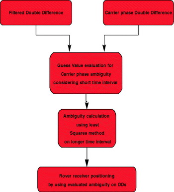
The block diagram of the algorithm presented is depicted in Figure 4 and in Figure 5 the deviation value is shown (argument of equation 7) given for different values of j in a real case. It is noted that the vertex of the parabola is given by the value of j equal to 1. In all the performed tests the vertex of parabola has been found for values of j ranging between ±2.
Algorithm for ambiguity resolution block diagram.

Standard deviation versus j.

Having identified the set of ambiguities (one for every DD) that provides the minimum standard deviation, it is used to calculate the baseline vector substituting smoothed DDs. Starting from this time for future positioning using the same set of satellites and within the same experiment, the ambiguities calculated are used with carrier phase double difference; pseudorange measurements are no longer required. This means that after a period of two minutes for GV evaluation, and after a period of about twenty minutes for ambiguity evaluation, the positioning can be obtained only by recording the carrier phase measurements.
3.2. Experimental results on static acquisition
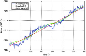
The proposed algorithm for solving carrier phase ambiguity was tested on a number of acquisitions performed simultaneously by two GPS receivers. The main results achieved are shown. First, in Figure 6, a comparison is sketched between pseudorange, smoothed and carrier phase with solved ambiguity DDs; the figure shows the different effect of noise in the three cases. From Figure 6 it is clear that the carrier phase DDs are less sensitive to noise than the smoothed ones. Moreover the latter are more accurate than the DDs evaluated by pseudoranges.
Comparisons between DDs evaluated by different methods.

In Figure 7 the x coordinate of GPS receivers baseline vector obtained with pseudorange DDs, with filtered DDs and with the ambiguity resolution on the carrier phase DDs, are sketched as an example showing the accuracies achievable on receiver positioning using these different methods. Figure 7 visualizes very well the increase in positioning accuracy achieved using smoothed or carrier phase double differences for DGPS. Even if the smoothing makes it possible to remove short period disturbances that affect pseudorange measurements it maintains the long period behaviour, affected by larger errors. Instead, the carrier phase DDs with solved ambiguities show a fixed value centred on smoothed DDs fluctuations. This is the main factor that influences the accuracy of results.
Details of the X coordinate of b obtained with pseudorange (left), smoothed (centre) and carrier phase (right) DDs.

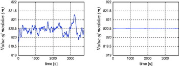
In Table 1 we show the calculated standard deviations of the three components of baseline vector derived from the pseudorange, filtered and carrier phase DD. The Table shows that the increase in accuracy achieved using smoothing with respect to simple pseudoranges is almost double. Using carrier phase ambiguity resolution the accuracy increases by two orders of magnitude! The final results, shown in Figure 8, are the random walk on the receivers module achieved by smoothing DDs and carrier phase DDs.
Modulus of b obtained by smoothed (left) and carrier phase (right) DDs.

Comparisons between the standard deviations obtained using different methods for DDs evaluation.

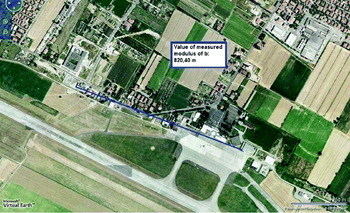
The baseline achieved module was compared to the value obtained through Google Maps (Figure 9) which confirmed the measurements achieved. In Figure 9 the effective positioning of the GPS receivers is also visible. One was positioned at the II Faculty of Engineering of the University of Bologna, the second one at the Ridolfi Airport of Forlì.
Modulus of b measured through Google Maps.

The standard deviations obtained on the calculation of the two modulus of baseline vector are:

3.3. Experimental results on dynamic acquisition
The proposed algorithm to solve the carrier phase ambiguity, after static tests, was verified on data provided during dynamic acquisition (rover GPS receiver moving). The GPS receiver located at the Forlì airport was chosen as reference receiver and the rover GPS receiver was mounted onboard a car. This experiment lasted about 45 minutes and was divided into six parts with:
• a preliminary static acquisition,
• a short tour of the car park, slow speed,
• a short tour of the car park, high speed,
• a long tour of the car park,
• a further static acquisition,
• an urban path.
Two static acquisitions were performed to test the calculation of ambiguities. The two short routes in the car park were used to set up the receiver hardware before the urban route. Moreover, the long car park tour was performed as a simulation of the urban route. Finally the real urban route was performed.
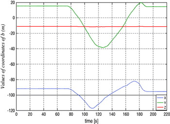
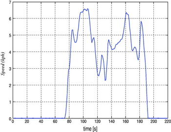
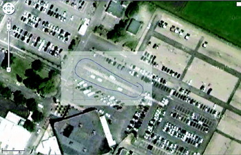
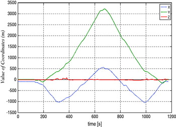
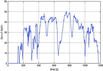
As an example, the components of the rover position with respect to a reference frame centred on the first receiver, the module of velocity and the reconstructed path superimposed on a terrain map are shown. Figure 10 shows the evolution of the coordinates of b and Figure 11 the velocity module during the test. Figure 12 shows the 2D reconstruction of the car trajectory. All results shown were achieved using only the carrier phase measurements and the ambiguities calculated during the first phase with the car not moving. The signal was sampled at a frequency of 1 Hz; the car speed was evaluated simply by determining the modulus of displacements between consecutive seconds.
Evolution of the coordinates of b during the short, low speed test tour.

Evolution of the car velocity module during the short, low speed test tour.

2D reconstruction of the car trajectory using carrier phase measurements and ambiguity resolution method proposed.

The final test was made by travelling along an urban route. Figure 13 shows the evolution of the coordinates of b and Figure 14 the car velocity. Some noise is present after about 300 seconds and after about 1000 seconds from the start. These positions correspond to a city tunnel where the contact with satellites was lost for a while.
Evolution of the coordinates of b during the urban route.

Car velocity measured during urban route experiment.

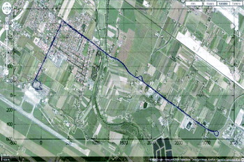
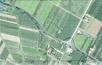
Figure 15 shows the 2D projection of the urban path. A zoom of the path is given in Figure 16 where the parallel lines of the two-way path are clearly visible. The roundabout in Figure 16 is lacking in the satellite terrain map (font: Google map) because the archive image is quite old.
Path of the urban route.

Detail of the trajectory of urban route.

4. CONCLUSIONS
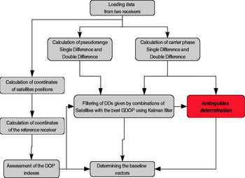
An algorithm able to determine the baseline vector (b) between two GPS receivers was presented. This algorithm first reduces noise that characterizes the pseudorange DDs using carrier phase DDs; in particular, the filter predicts the values of smoothed DDs merging the inaccurate but unambiguous DDs derived from pseudoranges with the extremely accurate but ambiguous carrier phase DDs. Then it calculates the carrier phase DDs ambiguities by applying a minimum square method to the first part of the acquired data. The main steps of this procedure are summarized in the flowchart in Figure 17.
Flowchart of developed algorithm.

The results achieved during algorithm application showed the limited accuracy of the results obtained from pseudorange measurements and the need for carrier phase measurements if high accuracy is required. In fact, using the pseudorange DDs for measuring the baseline, standard deviations ranging between 2 and 3 metres, depending on satellite GDOP, were achieved. Using the carrier phase DDs for filtering the pseudoranges the accuracy on baseline standard deviations increased by about 1 metre. Finally, using the algorithm presented for a rapid solution of carrier phase ambiguities an increase in accuracy of about two orders of magnitude was achieved. Standard deviations down to 2 centimetres were recorded during real applications.
All the conclusions in the paper were supported by the application to real cases and the data shown was derived from experiments carried out.
APPENDIX 1. RESOLUTION OF BASELINE VECTOR USING KALMAN FILTER FOR DDs
The smoothing of pseudoranges DDs through carrier phase DDs is achieved by applying the classical Kalman filter method as shown here.
This algorithm requires the mathematical model of the process to filter the measures; in this application the carrier phase DDs are used as the mathematical model of the measured pseudorange DDs. It is assumed that the carrier phase and pseudorange standard deviations can be described as white noise. It is then possible to assess:
• n the reference time,
• DD S− is the forecast of the value of filtered DD,
• DD cp is the carrier phase DD,
• DD pr is the pseudorange DD,
• q is the process noise evaluated from carrier phase standard deviation, obtained by multiplying cycles by the wavelength,
• r is the measured noise evaluated from pseudorange standard deviation,
• k is the filter gain,
• DD S+ is the value of filtered DD,
• p is the covariance.
The Kalman filter starts from:

In this equation, an estimate of the value of filtered DD at instant n is calculated by the sum of the value of filtered DD at time (n−1) plus the difference between the carrier phase DD, respectively, at time n and (n−1).
The second step of filtering is the evaluation of covariance at the instant of reference given by (A.2); this is achieved by taking into account both the predicted value of covariance and the process white noise:
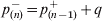
After the covariance evaluation, it is necessary to determine the filter gain (A.3) that assigns different weights to the measures (pseudorange DD) or to the mathematical model (carrier phase DD).
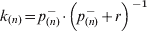
In the expressions A.4 and A.5 the value of filtered DDs and their estimated covariances are obtained:


After the smoothed DDs have been determined, it is necessary to calculate the matrix H that contains the differences of the satellite unit vectors referred to the corresponding filtered DDs; this is a matrix of 4 rows by 3 columns.
It is finally possible to determine the coordinates of the baseline vector (b) applying the following expression:

then, using the least squares, we obtain the value of b:

where:
• DD S is a column vector of four elements that consists of the filtered values of DD,
• H is the matrix (4×3) of unit vectors differences,
• b ECEF is the column vector whose three elements are the rover coordinates with respect to the reference receiver in the ECEF reference system.
The coordinate transformation from ECEF to SEU (South East Up) (Wertz, Reference James1980) reference system is given by A.8 where the reference GPS receiver latitude (L) and longitude (θ) are requested: