2.1. Description of GCP flow

A sketch of GCP flow is shown in figure 1 in a right-handed Cartesian coordinate frame $(x, y, z)$ with corresponding velocity components $(u,v,w)$. Here, $x$ is the wall-moving direction and $y$ is the wall-normal direction. The distance between the top wall and the bottom wall is $L_y = 2h$ while $L_x$ and $L_z$ are domain sizes in the $(x,z)$ directions, respectively. The top and bottom walls move in the $x$ direction with velocity components $(-U_c,0,0)$ and $(U_c,0,0)$, respectively. Misalignment between the pressure-gradient vector and the wall-velocity-difference vector results in volume flows in both the $(x,z)$ directions with characteristic velocities

(2.1a,b)\begin{equation} U_{Vx}=\frac{1}{2h}\int_{-h}^{h} U(y)\,{{\rm d}y},\quad U_{Vz}=\frac{1}{2h}\int_{-h}^{h} W(y)\,{{\rm d}y}, \end{equation}

with $U(y)$ and $W(y)$ volume-time-averaged mean-velocity profiles corresponding to velocity components $u$ and $w$. Other useful velocities are the resultant bulk velocity $U_V= ({{U_{Vx}}^2+{U_{Vz}}^2})^{1/2}$ and the general velocity scale $U_0= ({{U_c^2+ U_{Vx}}^2+{U_{Vz}}^2})^{1/2}$. The three velocities ($U_c \ge 0$, $U_{Vx}\ge 0$, $U_{Vz}\ge 0$) have associated Reynolds numbers

(2.2a–c)\begin{equation} Re_c = \frac{U_c h}{\nu},\quad Re_{Vx}=\frac{U_{Vx}h}{\nu},\quad Re_{Vz}=\frac{U_{Vz}h}{\nu}, \end{equation}

with $\nu$ the kinematic viscosity of the fluid.

Figure 1.

Sketch of generalized Couette–Poiseuille (GCP) flow. The separation distance between the top wall and the bottom wall is $L_y=2h$, while the domain sizes in $x$ and $z$ are $L_x$ and $L_z$, respectively. The wall-moving velocities of the top and bottom walls are $-U_c$ and $U_c$, as denoted by blue arrows. The angle $\phi =\arctan (Re_{Vz}/Re_{Vx})$ is the ratio of the volume flow in the $x$ and $z$ directions. The angle $\theta = \arctan [ (Re_{Vx}^2+Re_{Vz}^2)^{1/2}/Re_c ]$. Left and right blue lines show the projection of sketched velocity profiles in the $z$–$y$ plane and the $x$–$y$ plane.

The parameter set ($Re_c\ge 0$, $Re_{Vx}\ge 0$, $Re_{Vz}\ge 0$) forms the all-positive octant of a Cartesian space. It will be convenient to work with spherical coordinates $(Re, \theta, \phi )$ where

(2.3a–c)\begin{equation} Re_c = Re\cos \theta,\quad Re_{Vx} = Re\sin\theta\cos\phi,\quad Re_{Vz} = Re\sin\theta\sin\phi,\end{equation}

with inversion

(2.4a)$$\begin{gather} Re=\frac{U_0 h}{\nu}, \quad Re_V = \frac{U_V h}{\nu}, \end{gather}$$

(2.4b)$$\begin{gather}\theta=\arctan\left( \frac{Re_{V}}{Re_{c}}\right),\quad \theta \in [0^\circ, 90^\circ], \end{gather}$$

(2.4c)$$\begin{gather}\phi=\arctan\left( \frac{Re_{Vz}}{Re_{Vx}}\right),\quad \phi \in [0^\circ, 90^\circ]. \end{gather}$$

Here $Re_V$ is a Reynolds number corresponding to the resultant bulk velocity $U_V$ and $Re$ is taken as the defining global Reynolds number based on the general velocity scale $U_0$, $\tan \theta = U_V/U_c$ can be interpreted as the relative weighting of Poiseuille-type to Couette-type flow and $\phi$ denotes the angle made by the bulk velocity vector $(U_{Vx},0,U_{Vz})$ with the plate velocity-difference vector $(2U_c,0,0)$.

For $\theta =0^\circ$, $Re_{Vx}= Re_{Vz}= Re_V=0$ and the flow reduces to PC flow in the $x$ direction. When $\theta =90^\circ$, $Re_c =0$ and the flow becomes PP flow with net volume flow aligned with $\phi$. When $\phi =0^\circ$, both the plate velocity-difference vector and the volume-flow vector are aligned in the $x$ direction, as discussed by Cheng et al. (Reference Cheng, Pullin, Samtaney and Luo2023). This is PCP flow. When $\phi =90^\circ$, the volume-flow vector is perpendicular to the moving plates velocity-difference vector. This orthogonality results in a centrosymmetric ensemble-mean flow with the centre of symmetry at the origin of $(x,y,z)$ space, a property that exists only for $\phi =90^\circ$.

Sketches of typical mean-velocity profiles in both the $y$–$z$ plane and the $x$–$y$ plane are shown in figure 1. The flow along the $z$ direction behaves somewhat like a Poiseuille flow while the flow in $x$ resembles a $\phi =0^\circ$ flow described in previous studies of PCP flow. For the strictly laminar case, the flow degenerates to a linear combination of laminar Couette–Poiseuille flow in $x$ and Poiseuille flow in $z$. The exact solution and several typical profiles are described in Appendix A to illustrate the genuine three-dimensional feature of GCP flow.

Direct numerical simulations with specified $(Re, \theta, \phi )$ are expected to result in a statistically stationary turbulent flow with mean-velocity-profile vector $\boldsymbol {Q}=(U(y),0,W(y))$. For $\theta$ at or near zero, streamwise rolls exist and mean-velocity profiles can be defined that also depend on $z$, but this description is not considered presently. On the top and bottom walls, the shear stresses will each have vector form in the $(x,z)$ plane that can be expressed in skin-friction coefficient form $\boldsymbol {C_{ft}} = (C_{ft,x},C_{ft,z})$, $\boldsymbol {C_{fb}} = (C_{fb,x},C_{fb,z})$ with components

(2.5a–d)\begin{equation} C_{ft,x}=\frac{2\nu}{U_0^2}\eta_{t,x}, \quad C_{fb,x}=\frac{2\nu}{U_0^2}\eta_{b,x},\quad C_{ft,z}=\frac{2\nu}{U_0^2}\eta_{t,z},\quad C_{fb,z}=\frac{2\nu}{U_0^2}\eta_{b,z}, \end{equation}

where

(2.6a–d)\begin{equation} \eta_{t,x} = \left. \frac{\partial U}{\partial y} \right|_{t},\quad \eta_{b,x} = \left. \frac{\partial U}{\partial y} \right|_{b},\quad \eta_{t,z} = \left. \frac{\partial W}{\partial y} \right|_{t},\quad \eta_{b,z}= \left. \frac{\partial W}{\partial y} \right|_{b}, \end{equation}

and subscripts $t$ and $b$ refer to the top and bottom walls, respectively. These can also be expressed in polar form with magnitude and angle

(2.7a,b)\begin{equation} C_{ft}=\sqrt{C_{ft,x}^2 + C_{ft,z}^2},\quad \psi_t=\arctan\left( \frac{C_{ft,z}}{C_{ft,x}}\right),\quad \psi_t \in [0^\circ, 180^\circ], \end{equation}

where $\psi _t$ measures the angle between $\boldsymbol {C_{ft}}$ and the positive $x$ direction. Similarly, on the bottom wall,

(2.8a,b)\begin{equation} C_{fb}=\sqrt{C_{fb,x}^2 + C_{fb,z}^2},\quad \psi_b=\arctan\left(\frac{C_{fb,z}}{C_{fb,x}}\right),\quad \psi_b \in [0^\circ, 180^\circ]. \end{equation}

It is expected that when $\phi =0^\circ$, $C_{ft}$ and $C_{fb}$ reduce to $C_{ft,x}$ and $C_{fb,x}$, respectively. Cheng et al. (Reference Cheng, Pullin, Samtaney and Luo2023) define $C_{fb,x} > 0$ for Couette-type flow and $C_{fb,x} < 0$ for Poiseuille-type flow. Here there exists a special case with zero velocity gradient on the bottom wall (Coleman et al. Reference Coleman, Pirozzoli, Quadrio and Spalart2017) so that $C_{fb} =C_{fb,x} =0$ at a critical angle $\theta = \theta _t(Re)$. It will be seen that flows with $C_{bt,x} =0$ can be realized for non-zero $\phi$ but a resultant $C_{fb} =0$ exists only for $\phi =0^\circ$, which is parallel Couette–Poiseuille flow. All present GCP flows have $C_{ft}>0$.

We describe the mean-flow velocity $\boldsymbol {Q}(y)$ by its magnitude $Q(y)$ and angle $\psi _q(y)$ with respect to the $x$ axis as

(2.9a,b)\begin{equation} Q =(U^2+W^2)^{1/2},\quad \psi_q = \arctan\left(\frac{W}{U}\right),\quad \psi_q \in [0^\circ, 180^\circ]. \end{equation}

The resultant velocity vectors in the top- and bottom-wall reference frames can be defined as $\boldsymbol {Q_t}(y)=\boldsymbol {Q}(y)+(U_c,0,0)$ and $\boldsymbol {Q_b}(y)=\boldsymbol {Q}(y)-(U_c,0,0)$, respectively. The corresponding magnitudes and angles are given by

(2.10)\begin{equation} \left.\begin{gathered} Q_t(y)= \sqrt{(U(y)+U_c)^2+W^2(y)},\quad \psi_{q,t}(y)=\arctan\frac{W(y)}{U(y)+U_c},\\ Q_b(y)= \sqrt{(U(y)-U_c)^2+W^2(y)},\quad \psi_{q,b}(y)=\arctan\frac{W(y)}{U(y)-U_c}. \end{gathered}\right\} \end{equation}

We note, for consistency, that in the respective wall-stationary reference frames $\psi _{q,t}(-h)= \psi _t$ and $\psi _{q,b}(h)= \psi _b$.

The present DNS is implemented in terms of specified $(Re, \theta, \phi )$ corresponding to a global Reynolds number and specified volume-flow Reynolds numbers. The mean pressure-gradient vector is then a derived quantity. Its components in the $(x,z)$ directions, $\partial P/\partial x$ and $\partial P/\partial z$, can be obtained by time averages of the volume-integrated, wall-parallel momentum equations. In particular, the magnitude $d P/d r$ and the orientation of the mean pressure-gradient vector $\phi _P$ with respect to the $x$ axis are then given by

(2.11a,b)\begin{align} \frac{{\rm d} P}{{\rm d} r} =\sqrt{\left( \frac{\partial P}{\partial x}\right)^2 + \left(\frac{\partial P}{\partial z}\right)^2},\quad \phi_P(Re,\theta,\phi) = \arctan\left( \frac{\partial P}{\partial z}/ \frac{\partial P}{\partial x}\right) = \frac{ \eta_{z,t}+\eta_{z,b} }{ \eta_{x,t}+\eta_{x,b}}. \end{align}

For $\phi =0^\circ,\ \phi =90^\circ$, then $\phi _P = \phi$ but generally $\phi _P \ne \phi$.

2.2. Numerical methods and simulations performed

The DNS is performed by solving the incompressible Navier–Stokes equations

(2.12a,b)\begin{equation} \frac{\partial u_i}{\partial x_i} = 0,\quad \frac{\partial u_i}{\partial t}+ \frac{\partial u_iu_j}{\partial x_j} =-\frac{\partial p}{\partial x_i}+\nu\frac{\partial^2 u_i}{\partial x_j^2}, \end{equation}

within a box domain. Here $p$ is the instantaneous pressure divided by the constant fluid density. Boundary conditions in the $x$ and $z$ directions are spatially periodic, while Dirichlet boundary conditions $(u,v,w) = (U_c,0,0)$ at $y = -h$ and $(u,v,w) = (-U_c,0,0)$ at $y = h$ are used.

A third-order Runge–Kutta time marching technique is implemented combined with the fractional-step method to solve the equations. Conservation of kinetic energy is guaranteed using a staggered-grid strategy employing the skew-symmetric form of the convection term. The Fourier expansions in the $x$ and $z$ directions simplify the pressure-Poisson equation to a series of one-dimensional (1-D) linear Helmholtz equations while a dynamically adjusted time step of $\delta t$ satisfies the Courant–Friedrichs–Lewy condition. The overall numerical method has been validated by Cheng et al. (Reference Cheng, Pullin, Samtaney and Luo2023). The spatial domain $L_x \times L_y \times L_z = 8 {\rm \pi}\times 2 \times 8 {\rm \pi}$, with corresponding grid $1536 \times 160 \times 1536$, is square in the ($x$–$z$) plane owing to the presence of mean flow in both directions. A grid stretching strategy is adopted in the wall-normal direction as proposed by Cheng et al. (Reference Cheng, Pullin and Samtaney2022).

Cases implemented are shown as symbols in figure 2(a) within the spherical coordinate system $(Re, \theta, \phi )$. All lie on the surface of the sphere $Re=6000$ with uniform distribution in $(\theta,\phi )$ with an increment of $15^\circ$ in the range of $[0^\circ, 90^\circ ]$. When $\theta =0^\circ$, the total volume-flow rate is zero and the flow degenerates to a pure turbulent Couette flow in the $x$ direction.

Figure 2.

(a) Cases in spherical coordinates, with radius $Re$, polar angle $\theta$ and azimuthal angle $\phi$. All DNS have $Re = 6000$. (b) Summary of simulation parameters. Here $Re_{\tau }$ is the friction Reynolds number, $\Delta x^+$ is the dimensionless spacing in the $x$ direction and $\Delta y_{w}^+$ is the dimensionless spacing at both walls in the $y$ (wall-normal) direction. The subscripts $t$ and $b$ refer to the top and bottom walls, respectively, while the subscript $max$ refers to the maximum value across the range of $\theta$ cases at the particular $\phi$.

We also list some skin-friction-scaled flow parameters for cases in the table denoted figure 2(b). For every $\phi$, the maximum values for the skin-friction Reynolds number (defined below) are shown, and also the maximum dimensionless grid spacings, which are based on the skin-friction velocities. The relevant skin-friction velocities are defined by

(2.13)\begin{equation} \left.\begin{gathered} u_{\tau,t}= {\rm{sgn}}(-\eta_{t,x})\sqrt{ \nu\lvert \eta_{t,x} \rvert },\quad u_{\tau,b}= {\rm{sgn}}(\eta_{b,x})\sqrt{\nu \lvert \eta_{b,x} \rvert },\\ w_{\tau,t}={\rm{sgn}}(-\eta_{t,z}) \sqrt{\nu \lvert \eta_{t,z} \rvert },\quad w_{\tau,b}={\rm{sgn}} (\eta_{b,z}) \sqrt{\nu \lvert \eta_{b,z} \rvert }. \end{gathered}\right\} \end{equation}

Resultant skin-friction speeds can then be expressed as

(2.14a,b)\begin{equation} q_{\tau,t}= {\rm{sgn}}(u_{\tau,t}) \sqrt{(u_{\tau,t}^2+w_{\tau,t}^2)},\quad q_{\tau,b}= {\rm{sgn}}(u_{\tau,b}) \sqrt{(u_{\tau,b}^2+w_{\tau,b}^2)}. \end{equation}

Skin-friction Reynolds numbers and the dimensionless grid spacings on the top wall can be obtained as

(2.15a–d)\begin{equation} Re_{\tau,t}=\frac{q_{\tau,t}h}{\nu},\quad \Delta x^+_t=\frac{\Delta x q_{\tau,t}}{\nu},\quad \Delta y_{w,t}^+=\frac{\Delta y_{w} q_{\tau,t}}{\nu},\quad \Delta z^+_t=\frac{\Delta z q_{\tau,t}}{\nu}. \end{equation}

Quantities on the bottom wall, including $Re_{\tau,b}$, $\Delta x^+_b$, $\Delta y_{w,b}^+$, $\Delta z^+_b$, can be similarly defined. Tabulated values in figure 2(b) are for all cases with the particular $\phi$ shown. These indicate that the present DNS generally meets accepted criteria for pointwise convergence with respect to grid size. For example, the in-plane resolution is comparable to both Pirozzoli et al. (Reference Pirozzoli, Bernardini and Orlandi2014) and Lee & Moser (Reference Lee and Moser2018).

3.1. Skin-friction components

Figure 3(a) shows the skin-friction coefficient components $(C_{ft,x}, C_{ft,z})$ while figure 3(b) shows $(C_{ft}, \psi _t)$. Since the top wall moves in the negative $x$ direction, both $C_{ft,x}$ and $C_{ft,z}$ are positive. With increasing $\theta$, $C_{ft,x}$ is reduced as $Re_c$ decreases, while $C_{ft,z}$ increases with the increase of $Re_{Vz}$. The skin friction in PC flow $\theta =0^\circ$ is smaller than for PP flow $\theta =90^\circ$ owing to the definition of $Re$.

Figure 3.

Components of the skin-friction vector on the top wall for OCP flow with $\phi =90^\circ$. (a) In Cartesian coordinates $(C_{ft,x}$, $C_{ft,z})$. The black line is the skin-friction coefficient $C_{ft,x}$ in the $x$ direction, while the blue line is the skin-friction coefficient $C_{ft,z}$ in the $z$ direction. (b) In polar coordinates $(C_{ft},\psi _{t})$. The black line is the magnitude $C_{ft}$ calibrated by the left coordinate axis, while the blue line is the twist angle $\psi _{t}$ calibrated by the right axis.

In figure 3(b), $C_{ft}$ is the resultant skin friction and $\psi _{t}=\arccos ( C_{ft,x}/C_{ft})$ describes the angle between the top-wall skin-friction vector and the $x$ axis. As $\theta$ increases from $0^\circ$ to $15^\circ$, a small decrease of $C_{ft}$ is observed, which can be ascribed to the disappearance of large-scale roll structures observed in pure Couette flow ($\theta =0$). Further evidence will be discussed in § 6.2. When $\theta$ further increases from $15^\circ \to 90^\circ$, $C_{ft}$ generally increases with an increasing proportion or weighting of Poiseuille-type flow. It is interesting that the curve of $\psi _t$-$\theta$ is convex with $\psi _t>\theta$ except at $\psi _t=\theta =0^\circ$ for PC flow and $\psi _t=\theta =90^\circ$ for PP flow where $\psi _t =\theta$. This indicates coupling of the wall surface force and the externally applied pressure gradient for turbulent GCP flow, which is different to that for laminar flow.

3.2. Velocity profiles

Mean component velocity profiles scaled in outer variables using $U_0$ are shown in figure 4. When $\theta =0^\circ$, the $U/U_0$ mean-velocity profile conforms to pure Couette flow. As $\theta$ increases, $U(y)/U_0$ in figure 4(a) decreases with decreasing $Re_c$ eventually to zero for $\theta =90^\circ$. The mean spanwise velocity profile $W(y)/U_0$ is always symmetric, and approaches pure Poiseuille flow for $\theta =90^\circ$. As $\theta$ increases, the magnitude of $W(y)$ monotonically increases up to $\theta = 90^\circ$, when $Re_V = Re_{Vz}$.

Figure 4.

Mean-velocity profiles, $\phi =90^\circ$: (a) ${U}/{U_0}$. (b) ${W}/{U_0}$. Key: $\blacktriangle$: $\theta =0^\circ$, $\blacktriangledown$: $\theta =15^\circ$, $\blacktriangleleft$: $\theta =30$, $\blacktriangleright$: $\theta =45^\circ$, $\blacklozenge$: $\theta =60^\circ$, $\bullet$: $\theta =75^\circ$, $\blacksquare$: $\theta =90^\circ$. The black arrows indicate increasing $\theta$.

3.2.1. Mean-flow velocity magnitude $Q(y)$

The mean-flow velocity always lies in the $(x,z)$ plane but generally displays twist with respect to $(x,z)$ axes and with variation in the $y$ direction. In figure 5(a) the velocity magnitude is plotted as $Q_t^+$ vs $d_t^+$ with

(3.1a,b)\begin{equation} Q_t^+= \frac{Q_t}{q_{\tau,t}},\quad d_t^+= \frac{(h-y)q_{\tau,t}}{\nu}, \end{equation}

for $\theta = 0^\circ$–$90^\circ (15^\circ )$, where $q_{\tau,t}$ is defined by (2.14a,b). As $\theta$ increases from $0^\circ$ to $90^\circ$, the flow undergoes a change from PC to PP flow, and this is accompanied by some variation in the profiles in the nominal log region. According to some authors, parameters in the standard log law can differ for different canonical flows (Nagib & Chauhan Reference Nagib and Chauhan2008). In figure 5(a) the red dashed line is the log profile for PC flow, with $\kappa =0.41$ and $A=5.1$ obtained by Pirozzoli et al. (Reference Pirozzoli, Bernardini and Orlandi2014), while the red dash-dotted line is the component log law for PP flow, with $\kappa =0.384$ and $A=4.27$ as found by Lee & Moser (Reference Lee and Moser2015). When $\theta =0^\circ$ (pure Couette flow), $Q_t^+$ is in good agreement with the log law. When $\theta$ increases from $0^\circ$ to $15^\circ$, $Q_t^+$ first decreases and then increases as $\theta$ increases from $15^\circ$ to $90^\circ$. When $\theta =90^\circ$, the slope of the velocity profile is basically parallel to the reference line of a log law for Poiseuille flow.

Figure 5.

Inner-scaled velocity magnitude for OCP flow, $\phi =90^\circ$. (a) Scaled mean resultant velocity magnitude $Q_t^+$. Red dashed lines: log law with $\kappa =0.41$ and $A=5.1$ for Couette flow; red dash-dotted lines: $\kappa =0.384$, $A=4.27$ for Poiseuille flow. (b) Velocity gradient indicator function $\varXi _t$. Red dashed lines: reference lines of $1/0.41$; red dash-dotted lines: reference lines of $1/0.384$. See figure 4 for symbol key.

The velocity gradient indicator function $\varXi _t$ can be defined as

(3.2)\begin{equation} \varXi_t=d^+_t\frac{{\rm{d}}Q^+_t}{{\rm{d}}d^+_t}. \end{equation}

This is shown in figure 5(b) where there is a broad minimum value of approximately $1/0.41$ near $d_t^+\approx 60$ when $\theta =0^\circ$. This is interpreted presently as the onset of a log region. Our present $Re = 6000$ is perhaps not sufficiently large to see this more fully developed. When $\theta$ increases, this minimum first drops and then gradually rises.

The present computational domain is relatively shorter in the streamwise ($x$) direction and wider in the spanwise ($z$) direction, compared with typical PC flow simulation domains. To verify that the present domain provides accurate mean-velocity profiles, we compare the PC profile with $L_x\times L_y \times L_z = (8{\rm \pi} \times 2\times 8{\rm \pi} )$ at the same Reynolds number $Re=6000$ with data from Cheng et al. (Reference Cheng, Pullin, Samtaney and Luo2023) who used a similar computational domain to Lee & Moser (Reference Lee and Moser2018), $L_x\times L_y \times L_z = (20{\rm \pi} \times 2\times 6{\rm \pi} )$. As shown in figure 6, both the scaled mean resultant velocity $Q_t^+$ and the velocity gradient indicator function $\varXi _t$ agree well, providing validity of one-point diagnostics for the present simulations.

Figure 6.

Comparison of mean-velocity profile and indicator function for PC flow ($\phi =90^\circ$, $\theta =0^\circ$) at $Re=6000$ with Cheng et al. (Reference Cheng, Pullin, Samtaney and Luo2023). (a) Scaled mean resultant velocity magnitude $Q_t^+$. Dashed line: logarithmic law of $Q_t^+ = \ln d_t^+/0.41+5.1$. (b) Velocity gradient indicator function $\varXi _t$. Dashed line: reference line of $1/0.41$. Solid line: present DNS with $L_x\times L_y \times L_z = (8{\rm \pi} \times 2\times 8{\rm \pi} )$. Blue dotted symbols: Cheng et al. (Reference Cheng, Pullin, Samtaney and Luo2023) with $L_x\times L_y \times L_z = (20{\rm \pi} \times 2\times 6{\rm \pi} )$.

3.2.2. Component mean-flow profiles

The velocity components in the top-wall reference frame can be expressed in terms of $Q_t$ and the twisting angle $\psi _{q,t}$ as

(3.3a,b)\begin{equation} U+U_c= Q_t \cos \psi_{q,t},\quad W = Q_t \sin \psi_{q,t}, \end{equation}

while skin-friction velocities are related by

(3.4a,b)\begin{equation} u_{\tau,t}^2 = q_{\tau,t}^2\cos\psi_t,\quad w_{\tau,t}^2 = q_{\tau,t}^2\sin\psi_t, \end{equation}

where it is recalled that $\psi _t$ is the skin-friction angle at the wall. At the top wall $\psi _{q,t}(y=h)=\psi _t$ because the mean-flow streamlines are asymptotic to the skin-friction lines when $y\to h$.

We assume that a classical log region exists for $Q_t(y)$:

(3.5)\begin{equation} \frac{Q_t}{q_{\tau,t}}=\frac{1}{\kappa}\ln\left(\frac{ d_t q_{\tau,t}}{\nu}\right)+A.\end{equation}

We further make the approximation that the velocity-profile twist angle is constant and equal to its value at the wall, $\psi _{q,t}(y) = \psi _t$. This will be discussed later. From (3.3a,b), (3.4a,b) and (3.5) we can then obtain

(3.6)$$\begin{gather} U_t^+=\frac{\sqrt{\cos\psi_t}}{\kappa}\ln d_{x,t}^++{\sqrt{\cos\psi_t}}\left(A-\frac{\ln\sqrt{\cos\psi_t}}{\kappa}\right), \end{gather}$$

(3.7)$$\begin{gather}W_t^+=\frac{\sqrt{\sin\psi_t}}{\kappa}\ln d_{z,t}^++{\sqrt{\sin\psi_t}}\left(A-\frac{\ln\sqrt{\sin\psi_t}}{\kappa}\right), \end{gather}$$

where

(3.8a–d)\begin{equation} U_t^+=\frac{U+U_c}{u_{\tau,t}},\quad W_t^+=\frac{W}{w_{\tau,t}},\quad d_{x,t}^+= \frac{(h-y)u_{\tau,t}}{\nu},\quad d_{z,t}^+= \frac{(h-y)w_{\tau,t}}{\nu}.\end{equation}

These are referred to as modified component log relations.

Figure 7 shows mean-velocity components $U_t^+$ and $W_t^+$ scaled with $u_{\tau,t}$ and $w_{\tau,t}$, respectively, obtained from the DNS, each for $\theta = 0^\circ \unicode{x2013} 90^\circ (15^\circ )$. Also shown are red lines representing (3.6) and (3.7). These each use $(u_{\tau,t},w_{\tau,t})$ and $\psi _{q,t} = \psi _t$ obtained from the DNS for the various $\theta$ values. In figure 7(a) the red dashed lines are plotted with $\kappa =0.41$ and $A=5.1$ as discussed above for PC flow while in figure 7(b) the red dash-dotted lines are plotted with $\kappa =0.384$ and $A=4.27$ for PP flow.

Figure 7.

Mean-velocity components in the top-wall reference frame scaled with $u_{\tau,t}$ and $w_{\tau,t}$ for OCP flow with $\phi =90^\circ$. Plots of (a) $U_t^+$ vs $d_{x,t}^+$ and (b) $W_t^+$ vs $d_{z,t}^+$. See figure 4 for symbol key. The black arrows indicate increasing $\theta$.

In summary, the velocity magnitude exhibits a log region albeit, for the present $Re =6000$, with standard parameters that show a weak dependence on $\theta$ as the flow changes from Couette-like to Poiseuille-like as $\theta$ increases. The component mean-velocity profiles also exhibit log-like regimes with parameters that can be well estimated by approximating the mean-velocity angle of twist as the shear-stress angle at the wall in the reference frame where the wall is stationary.

4.1. Couette-type flow $90^\circ \leq \psi _{b} \leq 180^\circ$

Uppercase $U$ and $W$ denote model mean-velocity profiles in the laboratory reference frame. For Couette-type flow, we assume that the composite $U(y)$ mean-velocity profile comprises two pure log profiles relative to respective top and bottom walls, and then each transformed to the laboratory frame. These then join at a location $y=y_0$ to be determined. In the laboratory framework, the bottom-adjacent and top-adjacent profiles can then be expressed as

(4.1)$$\begin{gather} \text{I}: -h< y \le y_0: U(y) = U_c - q_{\tau,b} \cos\psi_b \left(\frac{1}{\kappa}\ln \left(\frac{( h+ y )|q_{\tau,b}|}{\nu}\right) +A \right), \end{gather}$$

(4.2)$$\begin{gather}\text{II}: y_0 \le y < h: U(y) =-U_c + q_{\tau,t}\cos\psi_t \left(\frac{1}{\kappa}\ln\left(\frac{(h - y )q_{\tau,t}}{\nu}\right) +A \right), \end{gather}$$

where $\kappa$ is the Kármán parameter and $A$ the offset constant.

For $W(y)$, we use the modelling profiles of Jones, Marusic & Perry (Reference Jones, Marusic and Perry2001) that here take the form

(4.3)\begin{align} & \text{III}: -h< y \le y_1: W(y)=-q_{\tau,b} \sin\psi_b \left[\frac{1}{\kappa}\ln\left(\frac{(h+y)|q_{\tau,b}|}{\nu}\right) +A \vphantom{\left(\frac{h+y}{h+y_1} \right)^2}\right. \nonumber\\ &\quad -\left. \frac{1}{3\kappa}\left( \frac{h+y}{h+y_1} \right)^3 +2\frac{\varPi}{\kappa} \left(\frac{h+y}{h+y_1} \right)^2 \left(3 - 2 \frac{h+y}{h+y_1}\right)\right], \end{align}

(4.4)\begin{align} & \text{IV}: y_1< y \le h: W(y)= q_{\tau,t} \sin\psi_t \left[\frac{1}{\kappa}\,\ln\left(\frac{(h-y)q_{\tau,t}}{\nu}\right) +A \vphantom{\left(\frac{h-y}{h-y_1} \right)^2}\right. \nonumber\\ &\quad -\left. \frac{1}{3\kappa}\left( \frac{h-y}{h-y_1} \right)^3 +2\frac{\varPi}{\kappa} \left(\frac{h-y}{h-y_1} \right)^2 \left(3 - 2 \frac{h-y}{h-y_1}\right)\right]. \end{align}

In the interests of constructing a relatively simple model, refinements such as pressure-gradient corrections in the wake function (Luchini Reference Luchini2018) have not been implemented. The two profiles join at the interior maximum point $y=y_1$, to be determined, where both have zero slope by construction. Cheng et al. (Reference Cheng, Pullin, Samtaney and Luo2023) found that this model profile worked well for $\phi =0^\circ$ except near $\theta - \theta _c$ small but non-zero where the flow near the bottom wall relaminarizes, before, as $\theta$ increases, transitioning back to turbulence. Since this effect is expected to be limited to a small region of $(\theta -\phi )$ space near $\theta = \theta _c$ and small $\phi$, and to shrink with increasing $Re$, then this is presently neglected.

When expressed in terms of Reynolds numbers, with $(Re,\theta,\phi )$ given, there are six unknowns: $Re_{\tau,b}$, $\psi _b$, $Re_{\tau,t}$, $\psi _t$, $y_0/h$ and $y_1/h$. Four equations are obtained from matching $U(y)$ and $\textrm {d} U/{\textrm {d}y}$ at $y=y_0$, $W(y)$ and $\textrm {d}^2W/{\textrm {d}y}^2$ at $y=y_1$ using the above profiles:

(4.5a,b)$$\begin{gather} U(y\to y_0^-) = U(y\to y_0^+),\quad \left.\frac{{\rm d} U}{{\rm d}y}\right|_{y_0\to y_0^-} = \left.\frac{{\rm d} U}{{\rm d}y}\right|_{y \to y_0^+}, \end{gather}$$

(4.6a,b)$$\begin{gather}W(y \to y_1^-) = W(y\to y_1^+),\quad \left.\frac{{\rm d}^2W}{{{\rm d}y}^2}\right|_{y\to y_1^-} = \left. \frac{{\rm d}^2W}{{{\rm d}y}^2}\right|_{y\to y_1^+}. \end{gather}$$

These give, respectively, after some algebra,

(4.7)\begin{gather} 2 \kappa Re \cos \theta - A\kappa (Re_{\tau,b} \cos\psi_b + Re_{\tau,t}\cos\psi_t ) - Re_{\tau,b} \cos\psi_b \ln (|Re_{\tau,b}| (1+Y_0)) \nonumber\\ -\,Re_{\tau,t}\cos\psi_t\ln (Re_{\tau,t}(1-Y_0)) =0, \end{gather}

(4.8)\begin{gather} Re_{\tau,b}\sin\psi_b [3 A K+6 P+3 \ln ( |Re_{\tau,b}| (Y_1+1))-1] \nonumber\\ \quad +\,[3A K+6 P+3\ln (Re_{\tau,t}(1-Y1))-1] Re_{\tau,t}\sin\psi_t=0, \end{gather}

(4.9)$$\begin{gather} Y_0 = \frac{Re_{\tau,b}\cos \psi_b - Re_{\tau,t}\cos\psi_t}{Re_{\tau,b} \cos\psi_b + Re_{\tau,t}\cos\psi_t}, \end{gather}$$

(4.10)$$\begin{gather}Y_1 = \frac{\sqrt{|Re_{\tau,b}|\sin \psi_b}-\sqrt{Re_{\tau,t}\sin\psi_t}}{\sqrt{|Re_{\tau,b}|\sin\psi_b}+\sqrt{Re_{\tau,t}\sin\psi_t}}, \end{gather}$$

where $Y_0 = y_0/h$ and $Y_1=y_1/h$. Two further closing equations are obtained by substituting (4.1), (4.2), (4.3) and (4.4) into (2.1a,b) to give $Re_{Vx}\equiv Re \sin \theta \cos \phi$ and $Re_{Vz}\equiv Re \sin \theta \sin \phi$. The mass-flux integration can be done and the resulting equations, with $Re$, $\theta$ and $\phi$ given, are

(4.11)\begin{align} & 2 \kappa Re ( \sin\theta \cos\phi - Y_0 \cos\theta) + Re_{\tau,b} (Y_0 + 1) \cos \psi_b ( A \kappa + \ln(|Re_{\tau,b}|(1 + Y_0)) - 1) \nonumber\\ &\quad + Re_{\tau,t} (Y_0 - 1) \cos \psi_t ( A \kappa + \ln(Re_{\tau,t}(1-Y_0)) - 1) = 0, \end{align}

(4.12)\begin{align} & 24 \kappa Re \sin \phi \sin \theta + Re_{\tau,b} (Y_1+1) \sin \psi_b (12 A\kappa +12 P+12 \ln (|Re_{\tau,b}| (Y_1+1))-13) \nonumber\\ &\quad +Re_{\tau,t} (Y_1-1) \sin \psi_t (12 A \kappa+12 P+12 \ln (Re_{\tau,t} (1-Y_1) ) -13)=0. \end{align}

Equations (4.7)–(4.12) describe Couette-type flow with $Re_{\tau,x,b}<0$. Near-wall viscous sublayer regions can be included at the cost of additional complexity, but the effect is negligibly small at values of $Re$ presently considered, even for near-bottom-wall flow when $|Re_{\tau,b}|$ is small.

For $\theta =0$, these equations have the exact solution $Re_{\tau,b} =-Re_{\tau,t}$, $Y_0=0$ and

(4.13)\begin{equation} Re_{\tau,t} = \frac{\kappa Re}{W ({\rm e}^{A\kappa} \kappa Re)}, \end{equation}

corresponding to pure Couette flow, where $W(Z)$ is the ProductLog function or Lambert function, which is the solution of $Z = W\ln (W)$. For given $Re$, $\theta$ and $\phi$, the six equations must generally be solved numerically with validity extended to $\psi _b = 90^\circ$, which is the limit of Couette-type flow in the streamwise direction.

4.2. Poiseuille-type flow $0^\circ \leq \psi _{b} \leq 90^\circ$

In this regime, all model profiles take the Jones et al. (Reference Jones, Marusic and Perry2001) log-wake form

(4.14)\begin{align} & \text{I}: -h< y \le y_0: U(y) = U_c + q_{\tau,b} \cos\psi_b \left[\frac{1}{\kappa}\ln\left(\frac{(h+y)q_{\tau,b}}{\nu}\right) +A \vphantom{\left(\frac{h+y}{h+y_0} \right)^2}\right. \nonumber\\ &\quad - \left. \frac{1}{3\kappa}\left( \frac{h+y}{h+y_0} \right)^3 +2\frac{\varPi}{\kappa} \left(\frac{h+y}{h+y_0} \right)^2 \left(3 - 2 \frac{h+y}{h+y_0} \right) \right], \end{align}

(4.15)\begin{align} & \text{II}: y_0 \le y < h: U(y) =-U_c + q_{\tau,t} \cos\psi_t \left[\frac{1}{\kappa}\ln\left(\frac{(h-y)q_{\tau,t}}{\nu}\right) +A \vphantom{\left(\frac{h-y}{h-y_0}\right)^2}\right. \nonumber\\ &\quad -\left. \frac{1}{3\kappa}\left( \frac{h-y}{h-y_0} \right)^3 + 2\frac{\varPi}{\kappa}\left(\frac{h-y}{h-y_0}\right)^2 \left(3 - 2 \frac{h-y}{h-y_0} \right) \right], \end{align}

(4.16)\begin{align} & \text{III}: -h< y \le y_1: W(y)= q_{\tau,b} \sin\psi_b \left[\frac{1}{\kappa}\,\ln\left(\frac{(h+y)q_{\tau,b}}{\nu}\right) +A \vphantom{\left(\frac{h+y}{h+y_1} \right)^2}\right. \nonumber\\ &\quad -\left.\frac{1}{3\kappa}\left(\frac{h+y}{h+y_1} \right)^3 +2\frac{\varPi}{\kappa} \left(\frac{h+y}{h+y_1} \right)^2\left(3 - 2 \frac{h+y}{h+y_1}\right)\right], \end{align}

(4.17)\begin{align} & \text{IV}: y_1< y \le h: W(y)= q_{\tau,t} \sin\psi_t \left[\frac{1}{\kappa}\ln\left(\frac{(h-y)q_{\tau,t}}{\nu}\right) +A \vphantom{\left(\frac{h-y}{h-y_1}\right)^2}\right. \nonumber\\ &\quad -\left. \frac{1}{3\kappa}\left( \frac{h-y}{h-y_1} \right)^3 +2\frac{\varPi}{\kappa} \left(\frac{h-y}{h-y_1}\right)^2\left(3 - 2 \frac{h-y}{h-y_1} \right) \right], \end{align}

and zero slope is automatic in both $U(y)$ and $W(y)$ profiles at $Y = Y_0, Y=Y_1$, respectively.

The velocity matching conditions for $U(y)$ and $W(y)$ are still $U(y\to y_0^-)= U (y\to y_0^+)$ and $W(y\to y_1^-)=W(y\to y_1^+)$, while the second-derivative matching conditions are now

(4.18a,b)\begin{equation} \left. \frac{{\rm d}^2 U}{{\rm d}y^2} \right| _{y\to y_0^-} = \left. \frac{{\rm d}^2 U}{{\rm d}y^2} \right| _{y\to y_0^+},\quad \left. \frac{{\rm d}^2 W}{{\rm d}y^2} \right| _{y\to y_1^-} = \left. \frac{{\rm d}^2 W}{{\rm d}y^2} \right| _{y\to y_1^+}. \end{equation}

Closure equations are again obtained by substituting (4.14), (4.15), (4.16) and (4.17) into (2.1a,b), and the mass flux integration can be done analytically. Details are omitted. A Poiseuille-type flow model is then obtained with six unknowns and six equations.

Numerical calculations were performed by first fixing $Re = 6000$ (but any large value can be used). For each $\phi$, with $\theta =0^\circ$, the solution strategy begins using the Couette-type model of (4.1). Solutions to the nonlinear equations were obtained numerically in a symbolic environment powered by MATHEMATICA$^{\circledR}$. As $\theta$ increases, the solution angle $\psi _b$ decreases from $\psi _b=180^\circ$ until, for some $\theta$, a solution with $\psi _b >90^\circ$ cannot be found. For this $\theta$, there is then a switch to the Poiseuille-type model equations of this section that are utilized until $\theta = 90^\circ$. This process is repeated for all $0\le \phi \le 90^\circ$ with $2.5^\circ$ increments. Numerical solutions were found without difficulty for all $(\phi,\theta )$ in the stated ranges. A quite small discontinuity in solution quantities exists in the change from the Couette-type to the Poiseuille-type equations as $\psi _b$ passes through $\psi _b=90^\circ$, but since this is expected to be smaller than the general accuracy of the model, it is ignored.

For $\theta =90^\circ$, the equations have $Re_{\tau,b}=Re_{\tau,t}$, $Y_0=Y_1=0$ and

(4.19)\begin{equation} Re_{\tau,t} = \frac{\kappa Re}{W (\exp({-13/12+ \varPi +A \kappa}) \kappa Re)}, \end{equation}

corresponding to pure Poiseuille flow.

5.1. Skin-friction components

Modelling results are calculated as described above, and then converted to skin-friction coefficients. Figure 8 shows the distributions of $C_{fb,x}$, $C_{fb,z}$, $C_{ft,x}$ and $C_{ft,z}$. Each red point denotes a DNS result while the blue surface is fitted to the model calculations. When $\theta =0^\circ$, the seven points contract to a single PC flow. Figure 8(a) shows $C_{fb,x}$ on the bottom wall. With $\theta =0^\circ$, $C_{fb,x}<0$ for PC flow. When $\theta$ increases, $C_{fb,x}$ crosses zero at a critical angle $\theta =\theta _c(\phi )\approx 37.5^\circ$. For $\theta >\theta _c$, $C_{fb,x}>0$ and increases with increasing $\theta$. Following Cheng et al. (Reference Cheng, Pullin, Samtaney and Luo2023), we define flow with $C_{fb,x}<0$ as Couette type and the flow with $C_{fb,x}>0$ as Poiseuille type. Figure 8(c) shows $C_{ft,x}>0$. When $\phi \ne 90^\circ$, the $x$ flow is driven by both moving walls and the $x$ component of the pressure gradient. With increasing $\theta$, $C_{ft,x}$ first increases and then decreases, consistent with the results of $Re_{\tau,t}$ in Cheng et al. (Reference Cheng, Pullin, Samtaney and Luo2023). This is not the case for $\phi = 90^\circ$, which shows a monotonic decrease in figure 3. Figure 8(b,d) shows $z$ skin-friction components. When either $\phi$ or $\theta$ gradually increase, both $C_{fb,z}$ and $C_{ft,z}$ increase with increasing volume flow in the $z$ direction. The modelling generally well predicts the trend of all these skin-friction components in the $(\phi,\theta )$ plane.

Figure 8.

Components of skin-friction coefficients in Cartesian coordinates. Red spherical points are from DNS at $Re =6000$. The blue is a surface fitted to model calculations with fine resolution in $(\theta -\phi )$ variables. Results are shown for (a) $C_{fb,x}$, (b) $C_{fb,z}$, (c) $C_{ft,x}$, (d) $C_{ft,z}$.

Figure 9 shows the skin friction at both walls in polar coordinates ($C_{fb}, \psi _b)$ and $(C_{ft},\psi _t)$. Symbols are DNS at discrete $(\phi,\theta )$, while the dashed lines are the corresponding model predictions. Figure 9(a) shows the skin-friction coefficient $C_{fb}$ on the bottom wall. For flows with small $\phi$, when $\theta$ is increased, $C_{fb}$ first decreases from the value for PC flow to a minimum, as a result of flow laminarization on the bottom wall near $\theta =\theta _c$ (Cheng et al. Reference Cheng, Pullin, Samtaney and Luo2023), and then increases to the PP limit. In contrast, on the top wall in figure 9(c), $C_{ft}$ first increases from the pure Couette–Poiseuille flow value to a maximum, and then decreases to pure Poiseuille flow as $\theta$ is increased, which is also consistent with the behaviour of $Re_{\tau,t}$ in Cheng et al. (Reference Cheng, Pullin, Samtaney and Luo2023). The limit $\theta \to 90^\circ$ corresponds to pure Poiseuille flow in the direction defined by $\phi$. Here $\psi _b, \psi _t \to \phi$, which is captured by both the DNS and the mean-flow model. There are quantitative discrepancies between the modelling and DNS for some components of $C_f$ over parts of $(\theta,\phi )$ space, which are attributable both to flow relaminarization near $\theta =\theta _c$, $\phi =0$ (not included in the model but implemented in Cheng et al. Reference Cheng, Pullin, Samtaney and Luo2023), and also to the fact that the model is a large-Reynolds-number approximation. But overall the modelling well captures the general trend of the DNS. The orientation angles $(\psi _b,\psi _t)$ are shown in figure 9(b,d), respectively. When $\phi =0^\circ$, we have PCP flow, where on the bottom wall at $\theta =\theta _c$, $\psi _b$ changes discontinuously from $180^\circ$ to $0^\circ$. When $\phi \ne 0^\circ$, the flow changes from PC-type flow to PP-type flow smoothly when $\psi _b = 90^\circ$ at an angle $\theta$ that depends on $\phi$ and that can be determined from figure 9(b).

Figure 9.

Skin friction in polar coordinates for both walls versus $\theta$ for different $\phi$. Filled symbols are from DNS and the dashed lines are the model results. Results are shown for (a) $C_{fb}$, (b) $\psi _b$, (c) $C_{ft}$, (d) $\psi _t$. Note that for $\theta = 90^\circ$, both $\psi _b, \psi _t \to \phi$. Key: ($\blacktriangle$, blue): $\phi =0^\circ$, ($\blacktriangledown$, blue): $\phi =15^\circ$, ($\blacktriangleleft$, blue): $\phi =30$, ($\blacktriangleright$, blue): $\phi =45^\circ$, ($\blacklozenge$, blue): $\phi =60^\circ$, ($\bullet$, blue): $\phi =75^\circ$, ($\blacksquare$, blue): $\phi =90^\circ$. The black arrows indicate increasing $\phi$.

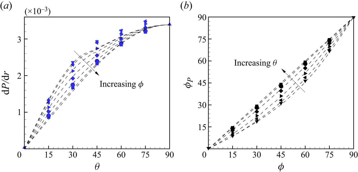
The DNS method fixes the volume-flow vector and not the mean pressure-gradient vector. Volume–time integration of (2.11a,b) shows that the resultant skin-friction forces are balanced by the mean pressure gradient. Figure 10 shows both the magnitude and direction $\phi _p$ of the mean pressure gradient, where the latter can be calculated using (2.11a,b). In pure Couette flow with $\theta =0^\circ$, there is a zero pressure gradient. When $\theta$ increases, $\textrm {d}P/\textrm {d}r$ increases with the growing proportion of Poiseuille flow, and reaches a maximum value at $\theta =90^\circ$. Except for relaminarization near $\theta =\theta _c$, the model captures the general trend of the DNS results. If Couette flow and Poiseuille flow are decoupled, as for laminar flow, the pressure-gradient vector is parallel to the mass-flow direction defined by $\phi$. But, as shown in figure 10(b), when $\phi \neq 90^\circ$, there is a small angle between $\phi$ and $\psi _p$, a result of ($x$–$z$) turbulent flow coupling.

Figure 10.

Magnitude and angle $\phi _P$ of the mean pressure-gradient vector. Filled symbols for DNS and dashed lines for model calculations. (a) Plot of $\textrm {{d}}P/\textrm {{d}}r$ vs $\theta$; see figure 9 for symbol key. (b) Plot of $\phi _P$ vs $\theta$; see figure 4 for symbol key.

5.2. Velocity profiles

Mean-velocity components scaled with $u_\tau$ and $w_\tau$ are shown in figure 11 for $\phi = 45^\circ$. The plots are in inner scaling relative to the respective top and bottom walls as defined by (3.8a–d). Also shown are modified log laws as red dashed and dash-dotted lines calculated with (3.6)–(3.7) using ($\psi _b,\psi _t$) values obtained from modelling and again assuming $\psi _{q,t} = \psi _t$ and $\psi _{q,b} = \psi _b$. The empirical log lines agree well with the DNS for the pure Couette flows and pure Poiseuille limits. Mean velocities $U_b^+$ and $U_t^+$ are shown in figure 11(a,c). When $\theta$ gradually increases from $0^\circ$ to $90^ \circ$, the DNS deviates from the log line for Couette flow and then returns to that for Poiseuille flow, which is consistent with the PCP flow DNS of Cheng et al. (Reference Cheng, Pullin, Samtaney and Luo2023). The $z$ mean-velocity profile $W_b^+$ is shown in figure 11(b), which first increases and then decreases with increasing $\theta$. Figure 11(d) shows $W_t^+$, which gradually increases with increasing $\theta$, and the log law fits well with all cases from $\theta =15^\circ$ to $\theta =90^\circ$.

Figure 11.

Mean-velocity components for top and bottom walls scaled with $u_\tau$ and $w_\tau$, respectively, for $\phi =45^\circ$. The modified log laws shown as red dash and dash-dotted lines are as calculated from (3.6), (3.7) using $\psi _b$, $\psi _t$ from the mean-flow modelling. Results are shown for (a) $U_b^+$, (b) $W_b^+$, (c) $U_t^+$, (d) $W_t^+$. Key: $\blacktriangle$: $\theta =0^\circ$, $\blacktriangledown$: $\theta =15^\circ$, $\blacktriangleleft$: $\theta =30$, $\blacktriangleright$: $\theta =45^\circ$, $\blacklozenge$: $\theta =60^\circ$, $\bullet$: $\theta =75^\circ$, $\blacksquare$: $\theta =90^\circ$. The black arrows indicate increasing $\theta$.

Figure 12 shows the resultant velocity magnitude scaled with $q_\tau$ and the velocity gradient indicator function for both walls. The log law is calculated in the same way as for figure 5. Figure 12(a,b) shows $Q_b^+$ and $Q_t^+$. Similar to the results of figure 11, deviation first from and then back to the empirical log law can be observed. The indicator functions $\varXi _b$ and $\varXi _t$ are plotted in figure 12(c,d). An incipient plateau near $1/0.41$ can be seen in pure Couette flow, while when $\theta =90^\circ$, the velocity gradient is around $1/0.384$, but the plateau is not well developed owing to the relatively low Reynolds number.

Figure 12.

Resultant velocity magnitude scaled with $q_{\tau }$ and velocity gradient indicator function for $\phi = 45^\circ$. The log relation is as for figure 5. Results are shown for (a) $Q_b^+$, (b) $Q_t^+$, (c) $\varXi _b$, (d) $\varXi _t$. See figures 4 or 11 for symbol key.

5.3. Mean-flow velocity vector twist

Twist behaviour of the resultant mean-velocity vector is a salient feature of GCP flow. The variation of the mean-velocity twist angle as a function of $y$ depends on the chosen frame of reference. For clarity, we denote twist angles by $\psi _q$ for the laboratory reference frame, $\psi _{q,t}$ for the reference frame with the top wall stationary and $\psi _{q,b}$ for the reference frame with the bottom wall stationary. In contrast, the shear-stress angles at each wall $(\psi _b,\psi _t)$ are frame independent. Owing to the boundary conditions at each wall, in the laboratory reference frame the twist angle limits are $\psi _q (y\to -h) \to 0^\circ$ while $\psi _q (y\to h) \to 180^\circ$ for almost all flows with the exception $\theta =90^\circ$ where $\psi _q (y)= \phi$.

5.3.1. Laboratory reference frame

For laminar flow, analysis of $\psi _q$ is straightforward and results are given in Appendix A. For turbulent flow, predictions of $\psi _q(y)$ in the laboratory reference frame can be obtained from the mean-flow modelling of § 4 by direct evaluation of the second equation of (2.5a–d), following numerical solution of the model equations for each $(\phi,\theta )$. Figure 13 shows the twist angle displayed as $\psi _q(y)$ for different $\theta$ at fixed $\phi$. Symbols are DNS values while the dashed lines show model results. Additional model results with $\theta = 1^\circ, 2.5^\circ, 5^\circ$ are also included outside the range of the DNS. The $\psi _q(y)$ plots show similar qualitative features to their equivalents for laminar flow as shown in figure 22 in Appendix A, but with different profile shapes.

Figure 13.

Mean-flow velocity twist angle $\psi _q$ as defined in (2.5a–d): (a) $\phi =90^\circ$, (b) $\phi =45^\circ$. Symbols, DNS results; see figures 4 or 11 for symbol key. Dashed lines, modelling results. Also shown are additional modelling results for $\theta =1^\circ$, $2.5^\circ$ and $5^\circ$ (from top to bottom with $y>0$). The black arrows indicate increasing $\theta$.

Results for antisymmetric flow in the $x$ direction ($u(-y) = -u(y)$) with $\phi =90^\circ$ are shown in figure 13(a) while figure 13(b) shows $\phi =45^\circ$ where the antisymmetry in $u(y)$ and symmetry in $w(y)$ are broken, In pure PC flow with $\theta =0^\circ$, then $\psi _q=0^\circ$ for $-1\le y<0$ and $\psi _q= 180^\circ$ in $0< y\le 1$, while for pure PP flows with $\theta =90^\circ$, $\psi _q=\phi$. On the centreline at $y=0$, $\psi _q=\phi$ can be observed for all flows. On the top channel half, at fixed $y>0$, $\psi _q$ reduces rapidly as $\theta$ is increased, a trend that is much stronger than for laminar flow at the same $\phi$. In the range $15^\circ \le \theta \le 75^\circ$, the strong variation in $\psi _q(y)$ at fixed $\theta$ is apparent. The modelling predictions fit quite well with DNS results with discrepancies mainly attributable to approximating $\psi _q$ by the top- and bottom-wall shear-stress vectors in the respective reference frames. This is now discussed.

5.3.2. Reference frame with wall stationary

Since, for $\phi =90^\circ$, the wall-moving velocity-difference vector is perpendicular to the volume-flow vector and the mean velocity shows symmetries, we consider only the top half-channel in the reference frame where the top wall is stationary. In this reference frame $\psi _{q,t} (y\to h) \to \psi _t$. In order to visually appreciate the twist behaviour, figure 14 illustrates the resultant mean-velocity vectors in $(U,W,y)$ space for $\phi =90^\circ$.

Figure 14.

(a–g) Mean-velocity vectors in the top-wall reference frame, $(U+U_c, W)$, for $\phi =90^\circ$ (OCP), with $\theta =0^\circ$, $15^\circ$, $30^\circ$, $45^\circ$, $60^\circ$, $75^\circ$, $90^\circ$. The red arrows denote DNS results, expanding an interpolating surface coloured red. The vertical blue plane aligns with $\psi _t$. (h) Twisting angle deviation ${\Delta }\psi _{q,t}(y)=|\psi _{q,t}(y)-\psi _t|$. Red dots are for numerical results and the blue surface for laminar flow.

In figure 14(a–g) three-dimensional velocity vectors $\boldsymbol {Q_t}(y)$ are shown as bundles of red arrows. These are interpolated with a red-coloured surface to show the twist behaviour, while the blue plane is a reference surface parallel to the wall skin-friction coefficient vector at angle $\psi _t$ on the top wall. When $\theta$ increases from the PC flow of figure 14(a), the surface deviates from the $x$–$y$ plane and finally approaches the $y$–$z$ plane at $\theta = 90^\circ$, which is PP flow in the $z$ direction. The reference skin-friction plane and the velocity plane are generally not parallel.

To quantify the twisting behaviour with wall distance, a twist angle deviation $\Delta\psi _{q,t}$ is defined as $|\psi _{q,t}(y)-\psi _t|$, the absolute angle difference between the velocity vector at $y$ and the wall skin vector. In figure 14(h) the red dots are the DNS results of ${\Delta }\psi _{q,t}(y)$ for $\phi =90^\circ$ and $Re=6000$, while the blue surface is the reference surface for laminar flow. The general trends of turbulent and laminar flows are similar, where ${\Delta }\psi _{q,t}$ gradually increases off from the wall. When $\theta$ increases from $0^\circ$, generally ${\Delta }\psi _{q,t}$ first increases and then decreases with increasing $\theta$, although the maximum value of $\Delta \psi _{q,t}$ in turbulent flows are much smaller compared with the laminar equivalents.

Figure 15 shows the three-dimensional resultant mean-velocity vector and deviation in the top-wall and bottom-wall reference frames for $\phi =45^\circ$. As in figure 14, the flow gradually changes from PC flow in the $x$ direction to pure PP flow at an angle of $45^\circ$. In figure 15(a,b) we plot only the mean-velocity vectors at $\theta =45^\circ$, which corresponds to the maximum deviation among cases with different $\theta$.

Figure 15.

Twist behaviour for GCP flow with $\phi =45^\circ$. (a) Mean-velocity vector $(U+U_c, W)$ in top-wall reference frame, (b) $(U-U_c, W)$ in bottom-wall reference frame, (c) twist angle deviation ${\Delta }\psi _{q,t}(y)$ in top-wall reference frame, (d) ${\Delta }\psi _{q,b}(y)$ in bottom-wall reference frame. See figure 14 for symbol key.

Figure 15(c,d) shows the deviation ${\Delta }\psi _{q,t}$ and ${\Delta }\psi _{q,b}$ for $\theta =0^\circ \sim 90^\circ$. In the top-wall reference frame (right), the rotation of mean-flow velocity vectors is substantially smaller and hard to recognize. In the bottom-wall reference frame (left), similarly as in figure 14, the deviation ${\Delta }\psi _{q,b}$ also first increases and then decreases with increasing $\theta$, while the maximum value is larger than that for $\phi =90^\circ$ flows.

6.1. Premultiplied one- and two-dimensional spectra

One-dimensional velocity spectra expressed in log-wavenumber coordinates have proven a powerful tool in the diagnostic analysis of canonical wall-bounded turbulent flows, suggesting the existence of $k^{-1}$ (Perry, Henbest & Chong Reference Perry, Henbest and Chong1986; del Álamo et al. Reference del Álamo, Jiménez, Zandonade and Moser2004; Lee & Moser Reference Lee and Moser2015) and $k^{-5/3}$ Kolmogorov-like regimes (see Perry et al. Reference Perry, Henbest and Chong1986). The premultiplied energy spectrum $k\varPhi (k)$ has the property that its integral with respect to the log-transformed wavenumber $\log_{10}k$ gives the turbulent kinetic energy. Premultiplied spectra are then useful in analysing the distribution of turbulent energy at different length scales. A striking example is the identification of very-large-scale, longitudinal structures at sufficiently large $Re_\tau$, as observed from their footprint in the wall-normal variation of the $k_x$ premultiplied spectrum of the streamwise velocity $\varPhi _{uu}(k_x)$ (Hutchins & Marusic Reference Hutchins and Marusic2007).

Although our $Re =6000$ is perhaps too low to produce the proposed $k^{-1}$ scaling range, we nonetheless explore premultiplied spectra for OCP flow with $\phi =90^\circ$ in order to investigate the scale distribution of kinetic energy and its changes with $\theta$ for this class of flows. For all cases, the centreline where $d_t^+ = h^+ = Re_\tau$ is on top of each coloured graph boundary. Figure 16 shows the $k_x$-premultiplied 1-D spectra as a colour-contour plot in ($\log _{10}d_t^+, \log _{10}(k_xh)$) coordinates for different $\theta$. Three columns show spectra of $(u,v,w)$ and the fourth shows the cross-spectrum of $u$ and $w$ computed as the magnitude of $\hat {u}(k)\hat {w}^*(k)+\hat {u}^*(k)\hat {w}(k)$, where the hat denotes the Fourier coefficient and the asterisk is the complex conjugate. The $k_x$-premultiplied 1-D spectra for PC flow with $\theta =0^\circ$ and PP flow with $\theta =90^\circ$ show similar features to the corresponding results of Lozano-Durán & Jiménez (Reference Lozano-Durán and Jiménez2014) and Lee & Moser (Reference Lee and Moser2018). As $\theta$ increases from $0^\circ \to 90^\circ$ in figure 16, spectra depict the transition from PC flow in the $x$ direction to PP flow in the $z$ direction. The $k_x\varPhi _{uu}$ spectrum shows a peak near $y^+\approx 15$ that moves in the increasing $k_x$ direction as $\theta$ increases, signalling the tendency towards smaller length scales as the $x$ axis changes from the effective longitudinal to the transverse direction. In figure 16(a,b) the width of the spectral humps for both $k_x\varPhi _{uu}$ and $k_x\varPhi _{vv}$ gradually decrease with increasing $\theta$, indicating that the distribution of energy is more concentrated over a narrower range of scales. The cross-spectrum $k_x\varPhi _{uw}$ shows a strong peak at $\theta = 45^\circ$.

Figure 16.

Contours of $k_x$-premultiplied 1-D spectra for OCP flow ($\phi =90^\circ$): (a) $k_xh\varPhi _{uu}/q_\tau ^2$, (b) $k_xh\varPhi _{vv}/q_\tau ^2$, (c) $k_xh\varPhi _{ww}/q_\tau ^2$, (d) $k_xh\varPhi _{uw}/q_\tau ^2$. From top to bottom: $\theta$ from $0^\circ$ to $\theta =90^\circ$ with increments of $15^\circ$.

The narrow low-wavenumber spike or band in $k_x\varPhi _{uu}$ that can be seen near $k_xh \approx 0.5$ for $\theta = 0^\circ$ corresponds to a length scale of about $12.5 h$. Direct numerical simulations at $Re_\tau =500$ by Lee & Moser (Reference Lee and Moser2018) show three similar low-wavenumber peaks with the strongest occurring at $k_xh \approx 0.4$. This agreement shows that the present computational domain, although relatively short in the $x$ direction, can nonetheless capture the principal features of streamwise flow structures.

One-dimensional $k_z$-premultiplied spectra are shown in figure 17. All spectra for pure Couette flow at $\theta =0^\circ$ show a narrow spike or band centred around small positive $\log_{10} (k_zh)$, which can be interpreted as the spectral signature of coherent streamwise rolls (Tsukahara, Kawamura & Shingai Reference Tsukahara, Kawamura and Shingai2006) whose mean spacing is of the order of several channel half-heights in the transverse (for $\theta =0^\circ$) $z$ direction, independent of the size of the computational domain (Cheng et al. Reference Cheng, Pullin and Samtaney2022). This spike persists slightly at $\theta = 15^\circ$ but is not present at larger $\theta$, indicating the attenuation of roll structures with increasing $\theta$.

Figure 17.

Contours of $k_z$-premultiplied 1-D spectra for OCP flows ($\phi =90^\circ$): (a) $k_zh \varPhi _{uu}/q_\tau ^2$, (b) $k_zh \varPhi _{vv}/q_\tau ^2$, (c) $k_zh \varPhi _{ww}/q_\tau ^2$, (d) $k_zh \varPhi _{uw}/q_\tau ^2$. From top to bottom: $\theta =0^\circ \unicode{x2013} 90^\circ$ with increments of $15^\circ$.

Premultiplied spectra $k_z \varPhi _{uu}$, $k_z \varPhi _{vv}$ and $k_z \varPhi _{ww}$ display a low-wavenumber peak. For $k_z \varPhi _{uu}$ and $k_z \varPhi _{vv}$, in pure PC flow with $\theta =0^\circ$, two peaks are visible. The greater peak in the narrow spike reaches a maximum value at the centreline, while for $k_x \varPhi _{ww}$, it reaches a maximum value at about $d_t^+=100$ and decreases to a smaller value at the flow centreline. When $\theta$ gradually increases from $0^\circ$, the peak in the narrow spike of all four spectra quickly disappears and can no longer be observed, which indicates the disappearance of the large-scale, streamwise oriented roll structures. In addition, it can also be observed that the shape of the energy spectrum changes from the Couette-type flow in the $x$ direction to the Poiseuille-type flow in the $z$ direction. For $k_z\varPhi _{uu}$ in figure 17(a), as $\theta$ increases, the flow in the $x$ direction gradually weakens, so the energy spectrum decreases correspondingly. In figure 17(b,c) showing $k_z\varPhi _{vv}$, $k_z\varPhi _{ww}$, as $\theta$ increases, the respective peaks near the wall gradually move in the direction of decreasing $k_z$, that is, towards of larger length scales, which accompanies a structural change in the spectra shape.

In the $\varPhi _{v-v}$ spectra portraits in both the $x$ and $z$ directions, for Couette-type flow at low $\theta$, the contours extend across the channel centreline, while in Poiseuille-type flow with large $\theta$, closed contours are observed. Similar phenomena have been shown by Lee & Moser (Reference Lee and Moser2018). These effects can be attributed to lower–upper half-channel flow symmetry changes and breaking that accompanies $\theta$ variations in the range $0^\circ < \theta < 90^\circ$, as the flow transitions from PC to PP flow with corresponding changes to flow structure. For pure PP flow ($\theta =90^\circ$), the mean-velocity profile is symmetric, resulting in zero turbulent shear stress at the channel centre and corresponding decreased wall-normal turbulent intensities. In contrast, for PC flow ($\theta =0^\circ$), the mean-$x$ velocity profile is antisymmetric about the flow centre plane. As a result, as shown in corresponding plots by Pirozzoli et al. (Reference Pirozzoli, Bernardini and Orlandi2014) in their DNS up to $Re_\tau =986$, the turbulent shear stress is finite at the centreline and the wall-normal turbulent intensity generally shows a plateau. For $\phi = 90^\circ$, for all $\theta$, the $x$-mean-velocity profile is antisymmetric while the mean $z$ profile is symmetric. For all other $(\theta,\phi )$, component mean-velocity profiles display no symmetry/anti-symmetry properties.

The $k_x$- and $k_z$-premultiplied two-dimensional (2-D) spectra at approximately $d_t^+=30$ are shown in figure 18. The peaks of both $k_xk_z\varPhi _{uu}$ and $k_xk_z\varPhi _{vv}$ reach respective maxima with respect to $\theta$ variation at $\theta \approx 30^\circ$, $k_xk_z\varPhi _{uw}$ achieves a maximum value at $\theta =45^\circ$, while $k_xk_z\varPhi _{ww}$ maximizes at $\theta =60^\circ$. With an increase in $\theta$, rotation of spectra footprints in the $(\log_{10} (k_xh)-\log_{10} (k_zh))$ plane can be clearly observed. For example, as $\theta$ increases, the elongated $k_xk_z\varPhi _{vv}$ hump rotates from near alignment with the $\log_{10} (k_zh)$ axis towards alignment with the $\log_{10} (k_zh)$. At $\theta =45^\circ$, the spectrum shape is almost symmetric about $\log_{10} (k_zh)=\log_{10} (k_xh)$. This demonstrates the reorientation of energetic structures during the transition from Couette to orthogonal Poiseuille flow.

Figure 18.

Contours of $k_x$- and $k_z$-premultiplied two-dimensional (2-D) spectra at around $d_t^+=30$: (a) $k_xk_zh^2\varPhi _{uu}/q_\tau ^2$, (b) $k_xk_zh^2\varPhi _{vv}/q_\tau ^2$, (c) $k_xk_zh^2\varPhi _{ww}/q_\tau ^2$, (d) $k_xk_zh^2\varPhi _{uw}/q_\tau ^2$. From top to bottom: $\theta$ from $0^\circ$ to $\theta =90^\circ$ with increments of $15^\circ$.

Centreline ($\kern0.09em y=0$) $k_x$- and $k_z$-premultiplied, 2-D spectra are shown in figure 19. The peaks of both $k_xk_z\varPhi _{uu}$ and $k_xk_z\varPhi _{vv}$ reach a maxima at $\theta =15^\circ$, while both $k_xk_z\varPhi _{uw}$ and $k_xk_z\varPhi _{ww}$ reach a maxima at $\theta =30^\circ$. The low-wavenumber peak of $k_xk_z\varPhi _{uu}$ can be clearly observed in figure 19(a,d), which is consistent with the result in figure 17. Compared with figure 18, the rotation of overall premultiplied spectra can still be observed, but the rotation angle is smaller.

Figure 19.

Contours of the $k_x$- and $k_z$-premultiplied 2-D spectra on the centre line $y=0$: (a) $k_xk_zh^2\varPhi _{uu}/q_\tau ^2$, (b) $k_xk_zh^2\varPhi _{vv}/q_\tau ^2$, (c) $k_xk_zh^2\varPhi _{ww}/q_\tau ^2$, (d) $k_xk_zh^2\varPhi _{uw}/q_\tau ^2$. From top to bottom: $\theta$ from $0^\circ$ to $\theta =90^\circ$ with increments of $15^\circ$.

6.2. Large-scale features in GCP flows

To observe the large-scale flows more clearly, visualization of time-averaged $Q$ fields coloured by vertical velocity $v$ are shown in figure 20 for OCP flows with $\phi =90^\circ$. Here,

(6.1)\begin{equation} Q=-\frac{1}{2}\left[\left(\frac{\partial u}{\partial x}\right)^2+ \left(\frac{\partial v}{\partial y}\right)^2+ \left(\frac{\partial w}{\partial z}\right)^2\right]- \frac{\partial u}{\partial y}\frac{\partial v}{\partial x}- \frac{\partial v}{\partial z}\frac{\partial w}{\partial y}- \frac{\partial w}{\partial x}\frac{\partial u}{\partial z}, \end{equation}

which is commonly used for vortex identification. The images are a time average of the instantaneous flow field. Four flows are illustrated, each viewed from above the top plate with $\theta =0^\circ,\ 15^\circ, 30^\circ,\ 45^\circ$. Each figure displays the whole computational domain with the same scale in the three coordinate directions. Isosurfaces with $Q=0.01$ are plotted and coloured by the wall-normal velocity over ranges tailored for each specific flow.

Figure 20.

Visualization of time-averaged $Q$ fields coloured by vertical velocity $v$ for OCP flow with $\phi =90^\circ$. Here $Q=0.01$ for all cases. Results are shown for (a) $\theta =0^\circ$, (b) $\theta =15^\circ$, (c) $\theta =30^\circ$, (d) $\theta =45^\circ$.

In figure 20(a) with $\theta =0^\circ$, which is pure Couette flow in the $x$ direction, large-scale roll structures, each of which extends to both walls, meander along the $x$ direction. In the $8{\rm \pi}$ domain in the $z$ direction, five roll pairs are captured, which is consistent with the DNS of Pirozzoli et al. (Reference Pirozzoli, Bernardini and Orlandi2014). Since the view is from above the upper wall, which is moving in the negative $x$ direction, then the mean-flow velocity angle for $y>0$ is $\psi _q = 180^\circ$. When $\theta$ increases to $\theta =15^\circ$ in figure 20(b), the rolls are obliterated and very-large-scale structures are not visible. Figure 13 shows a very rapid change (decrease) in $\psi _q$ from $180^\circ$ at a $y>0$ level in the upper half-channel (where structures are most visible in the view shown), when $\theta$ increases in the range $0^\circ \unicode{x2013} 45^\circ$. This can be seen in figure 20(b) where visible isosurfaces in $y>0$ are oriented at $\psi _q \approx 135^\circ \unicode{x2013} 140^\circ$, which is largely towards the viewpoint.

Further increase of $\theta$ implies increased volume flow in the $z$ direction. In figure 20(c), $\psi _q$ in the upper half-channel has rotated further towards the $z$ axis, which continues at $\theta = 45^\circ$ in figure 20(d). Here, owing to enhanced transparency within the view, an averaged orientation difference between $Q$ isosurfaces in the upper and lower half-channel subdomains can be perceived. Still further increases in $\theta$ show $Q$-isosurface fields (not shown) that, from the chosen viewpoint, resemble those obtained for pure PP flow.

Visualizations of GCP flows with $\phi \ne 90^\circ$ and varying $\theta$ show similar structural changes to those seen in figure 20 but with differing fine details. Their novel, salient features not seen in parallel wall-bounded flows is the wall-normal rotation in structure orientation. A detailed study of the physics underlying cross-flow interactions in the presence of wall-normal, mean-velocity twist would seem of interest to understanding the physics of three-dimensional, wall-bounded turbulent flows. This would require new diagnostic and interpretive techniques, which is beyond the scope of the present investigation.