

1 Introduction
There has been a dramatic increase in women's labor supply in the US and several developed countries since the beginning of the 20th century [Goldin (Reference Goldin2006)]. During this period, women's labor force participation rate (LFPR) increased by almost 70 percentage points, narrowing the gender gap in labor force participation (LFP), as women benefited from rising education accompanied by more favorable gender wage ratio, technological innovations which allowed them control over the timing of child-birth and reduced time in home production activities [Goldin and Katz (Reference Goldin and Katz2000), Greenwood et al. (Reference Greenwood, Seshadri and Yorukoglu2005)]. In contrast to the western experience, similar socio-economic transitions have not necessarily resulted in lowering the gap between female and male LFPR significantly in developing countries.Footnote 1 Furthermore, the low levels of women's LFP are often accompanied by a non-monotonic relationship between their workforce participation and education, unlike in the OECD [OECD (2012)].Footnote 2 In contrast, men's labor supply is typically high and unchanged across all education levels in both developed as well as in low-income economies.
We highlight these features of women's LFP observed in several developing countries—the wide gender gap and the non-monotonic relationship between women's workforce participation and education—by theoretically modeling a married couple's time allocation decisions. We incorporate not just home production, as in standard models of household decision-making, but also allow for home productivity to improve with education in a collective decision-making framework following Chiappori (Reference Chiappori1988). Thus, agents derive utility from consumption, leisure, and a home good which is enjoyed jointly by the two-member household. Individuals may differ in terms of their education level, which we assume is exogenously determined before agents form the household.
A crucial feature of our model, therefore, is that the education level of the agents not only determines market productivity or the wages that they earn, but also their productivity at home. Hence, there are two possible channels through which couples’ labor supply decisions could be affected in our model—market productivity (gender wage gap) and home productivity, as education changes.Footnote 3 We show theoretically that, with an increase in the education level of women, the gender wage ratio may also move in their favor. But while a favorable relative wage encourages women's LFP, the accompanying rise in home productivity due to women's higher education also demands greater participation in the production of the home good. The net effect on the labor supply of women to market work is then determined by the relative strength of these two opposing forces.
In addition, we borrow from the vast literature on status consumption [Duesenberry and Press (Reference Duesenberry1949)] to incorporate a social norm on production of the home good as a third channel that affects couples’ labor supply decisions. Specifically, we include individual preferences on the extent to which the household deviates from the social norm of a benchmark level of the home produced good—child quality characterized by household expenditure on education.Footnote 4 Thus, households build status through production of a good that society values—the higher the home good production relative to the social norm or benchmark, the higher the utility the individual derives. In this unrestrictive theoretical framework, we do not place any constraints on how much time either the husband or the wife devotes to home production. Thus the social norm on the home good is gender neutral.Footnote 5
We calibrate this model with time use and consumption expenditure data from urban India and simulate it to match the observed data on married women's and men's time on market work, home production, and leisure. In urban India, we observe a fall in married women's time spent in the labor market between illiterate and middle education levels and a slight increase thereafter for higher secondary and graduate and above education levels. We show that in our model with the social norm on home production, and improvements in both market and home productivity with education, we are able to replicate both the observed non-monotonicity or U-shaped LFPR of women—fall in women's labor supply to market work at low and moderate levels of education and a rise at higher levels of education. The calibration exercise shows that fall in relative female wage along with an increase in relative female home productivity between illiterate to less than primary explains the fall in wife's labor market time upto middle education. The muted increase in female labor time for higher education levels is explained by a large increase in relative female home productivity and bargaining power within the household between middle to higher education levels. Our theoretical predictions, therefore, match the observed data on market work and home production better than a standard model with constant home productivity and no social norm.
Our analysis suggests that home production and social norms on a benchmark level of the home good may act as a constraint on wives’ decision to supply labor for market work. While the gender wage ratio plays an important role in determining both married men and women's labor supply across the distribution of education, it alone is unable to match women's labor supply at high levels of education.Footnote 6 Besides several sensitivity checks through varying parameter values, we also test for alternative mechanisms such as non-availability of modern technology or of market goods for home production and wealth effects to explain the observed patterns in women's LFP in India. These mechanisms fail to explain the observed regularities in the data.
Existing theoretical models that incorporate home production focus on the experience of developed countries and suggest that a rise in women's wages [Attanasio et al. (Reference Attanasio, Low and Sánchez-Marcos2008), Siegel (Reference Siegel2017)] and education or human capital [Olivetti (Reference Olivetti2006), Gobbi (Reference Gobbi2018)], relative to men's, should be accompanied by higher time in the labor market, with ambiguous effects on their home production and leisure time. In contrast to this literature, which includes home production either broadly or as child care, we develop a model that allows for education to affect productivity at home of both husbands and wives. Our model, where households jointly derive utility from home good, is backed by micro evidence from developing countries that education makes women (and possibly men) more productive in the home. For instance, Behrman et al. (Reference Behrman, Foster, Rosenzweig and Vashishtha1999) find that because households with an educated male member earned larger farm profits during the green revolution period in India (1968–1982), the returns to investing in male education increased. This, in turn, increased the demand for educated women in the marriage market with children of more educated women spending greater time at home studying, relative to the less educated mothers. Lam and Duryea (Reference Lam and Duryea1999) show that as Brazilian women get more schooling, total fertility falls and wages rise, but the share of women working does not increase. They conjecture that home productivity effects may be large enough to offset increases in market wages up to the first eight years of education.
A relatively small but increasingly relevant literature suggests there can be social factors and norms that affect decision-making of agents in an economy and thereby impact economic development [Chakraborty et al. (Reference Chakraborty, Thompson and Yehoue2015), Bernhardt et al. (Reference Bernhardt, Field, Pande, Rigol, Schaner and Troyer-Moore2018)]. Contextually, social constraints are likely to be even more relevant in a developing country, particularly as income levels rise and households seek social mobility. Social norm and status goods have been analyzed extensively in the literature in various contexts [e.g., Abel (Reference Abel2006)]. Goldin (Reference Goldin1994), in her seminal work, indicates that social and cultural factors can play a large role in married women's labor supply decisions while Fernández (Reference Fernández2013) models the link between cultural change and the evolution of women's LFP in the United States. While the microeconomic literature has theorized on gender-specific norms where men derive disutility from their wives working [Fernández et al. (Reference Fernández, Fogli and Olivetti2004), Bertrand et al. (Reference Bertrand, Cortes, Olivetti and Pan2020)], to the best of our knowledge, this is the first paper that explicitly models a (gender neutral) norm on home good production in an aggregate macroeconomic framework. We are able to show that even in a framework with no constraints on gender preferences, with households deriving a disutility if the production of the home good falls below a social benchmark, we can closely approximate the observed labor supply of married men and women.Footnote 7
Our findings build on previous work by Afridi et al. (Reference Afridi, Dinkelman and Mahajan2018) and Lam and Duryea (Reference Lam and Duryea1999) who highlight the U-shaped relationship between women's LFP and own education, and provide suggestive evidence of the role of home productivity in explaining this observed pattern. In contrast, we provide a theoretical framework to explain the mechanism through which home productivity can influence women's LFPR and calibrate the model to see the extent to which it can explain the U-shaped pattern of female LFPR with education. Furthermore, our analysis is able to show that norms enforced by society on the production of the home good may be an additional factor that explain the variation in married women's labor supply with their education. Specifically, we focus on production of a benchmark minimum human capital of the child within marriage, and show that even in the absence of gendered division of time, women may spend more time on domestic work and less in the market.Footnote 8
The paper is organized as follows. In section 2 we present some of the key facts regarding women's labor supply in India and describe the data. The theoretical model, based on collective decision-making, is formulated in section 3. In section 4 we calibrate and simulate our theoretical models. Section 5 discusses the contribution of three channels—gender wage ratio, home productivity, and social norms—in explaining married men and women's labor supply across the entire education distribution. We examine alternative mechanisms that can explain changes in women's LFP with education in section 6, while sensitivity checks on the simulations are reported in section 7. Section 8 concludes.
2 Background and data
In this section we first present the stylized facts on married women's and men's labor supply in urban India. We use multiple rounds of the National Sample Survey (NSS) of India, which are conducted to capture employment every few years.Footnote 9 We restrict our attention to urban, married women, and men in the economically productive age group of 20–45 years throughout. Note, however, that the facts we highlight here are equally applicable to a wider demographic group of men and women in India.Footnote 10
Educational attainment has been increasing in India. In 1999, more than 30% of women were illiterate, while the majority of men had at least secondary or higher secondary education. Between 1999 and 2011, educational attainment improved for both men and women, but the improvement was more dramatic for women. The proportion of illiterate men and women (married and in age group 20–45) in urban India fell by 6% and 12%, respectively, during 1999–2011. On the other hand, during the same time period, the proportion completing secondary schooling or more increased by 8% for men compared to 13% for women. Hence, the gender gap in higher educational attainment narrowed significantly from 12% to 7%.
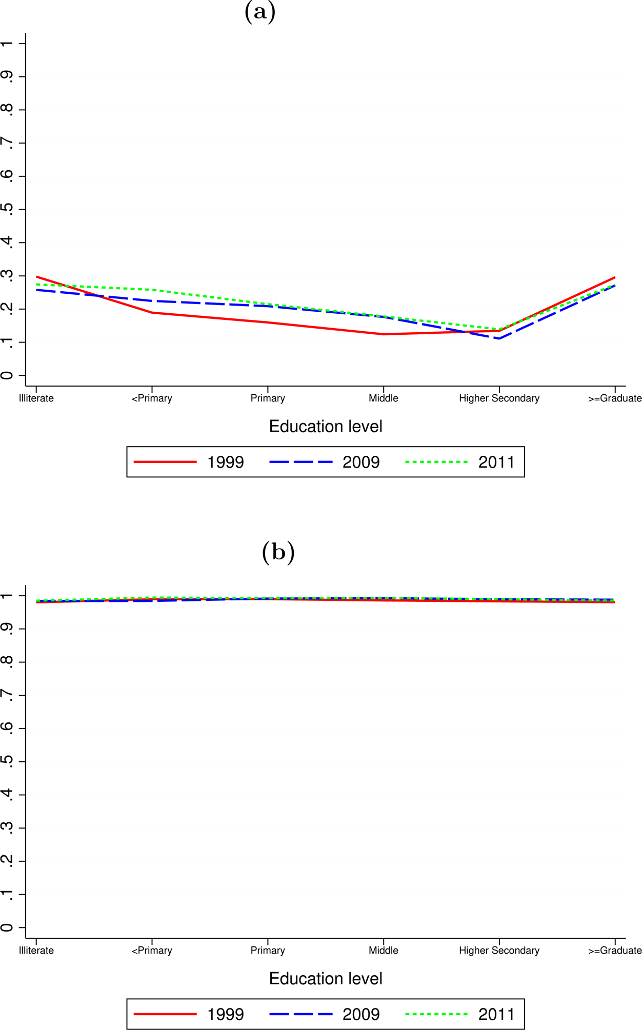
But while the gender gap in educational attainment has declined, there is almost no change in the LFPRs of women in urban India [Klasen and Pieters (Reference Klasen and Pieters2015)]. Married women in the 20–45 age group have shown very low levels of LFPR, at around 22%—unchanged across the last three decades. Typically, their LFPR declines marginally as education increases from illiterate to middle-higher secondary and then increases slightly at graduate and above (Figure 1). Overall, the LFPR of women is a U-shape, with a mild curvature, across education groups—a relationship that remains unchanged since the earliest data available in 1983.Footnote 11 Almost all married men on the other hand, were engaged in the labor market during the same period, irrespective of their education level (Figure 1).
LFPR by education (urban, married, age 20–45). (a) Women, (b) men. Source: National Sample Survey, Employment and Unemployment Schedules 1999, 2009, and 2011 (Authors’ own calculations). Note: LFPR is calculated using the usual status definition of employment in the NSS data. The sample size is 33,387 (in 1999), 26,103 (in 2009), and 25,864 (in 2011) for men and 37,732 (in 1999), 30,851 (in 2009), and 30,512 (in 2011) for women. See data appendix for details.
The above stylized fact may partly be explained by gender gap in market returns to education or market productivity (wages). However, as Figures 2(a–b) show the average real wages increase dramatically at higher levels of education for both married men and women. Moreover, the ratio of female to male wages rises (gender wage ratio) was significant at higher levels of education [Figure 2(c)]. This rise can also be seen in the ratio of female wage to the wage of their spouses (Appendix Figure A.2).Footnote 12 Thus, the non-responsiveness of more educated married women to the increase in their wages is puzzling. This non-responsiveness of married women becomes especially stark when we compare them to single women in the same age group (Figures A.3 and A.4, in Appendix A).Footnote 13 Single women not only have a higher level of LFPR than married women, but a larger proportion of these women work as their education levels and corresponding wages rise. On the other hand, married and single men do not behave very differently in terms of their LFPR across education groups.
Returns to education (urban, married, age 20–45). (a) Women, (b) men, (c) gender wage ratio. Source: National Sample Survey, Employment and Unemployment Schedules 1999, 2009, and 2011 (Authors’ own calculations). Note: Mean daily wage is calculated from the NSS data for each education-gender cell and deflated at 1999 price levels using the All India Consumer Price Index for Industrial Workers. The sample size is 17,466 (in 1999), 13,876 (in 2009), and 13,686 (in 2011) for men and 3569 (in 1999), 3064 (in 2009), and 3032 (in 2011) for women. The wage gap is calculated as the ratio of mean female and mean male wage rate.

These observations hold across each cross-section, indicating more or less stable, low levels of labor supply by women and almost no responsiveness to the improvement in the gender wage ratio in the cross-section and between 1999 and 2011. This is in sharp contrast to the western experience, elucidated by Goldin (Reference Goldin2006). To summarize, the following facts appear to be salient over the last few decades in urban India:
Fact 1: As women's education level increases in urban areas, the proportion of married women of age 20–45 working in the labor market decreases and then increases marginally. The overall labor force participation of women has been stagnant at 25%.
Fact 2: As men's education level increases in urban areas, the proportion of married men of the same age group who are working in the labor market stays very high (above 95%) and flat.
Fact 3: Real mean wages rise both for women and men with their education. But across the education categories, the largest increase is for graduate and above category of education, and more so for women.
Given the fact that men and women's labor force attachment, both overall and by education, isrelatively unchanged across the decades between 1999 and 2011, we henceforth focus on the urban sample of the nationally representative Time Use Survey (TUS) in 1998 for the same demographic group mentioned above.Footnote 14 The TUS data allow us to investigate the relationship between education and allocation of time to market work, home production, and leisure.
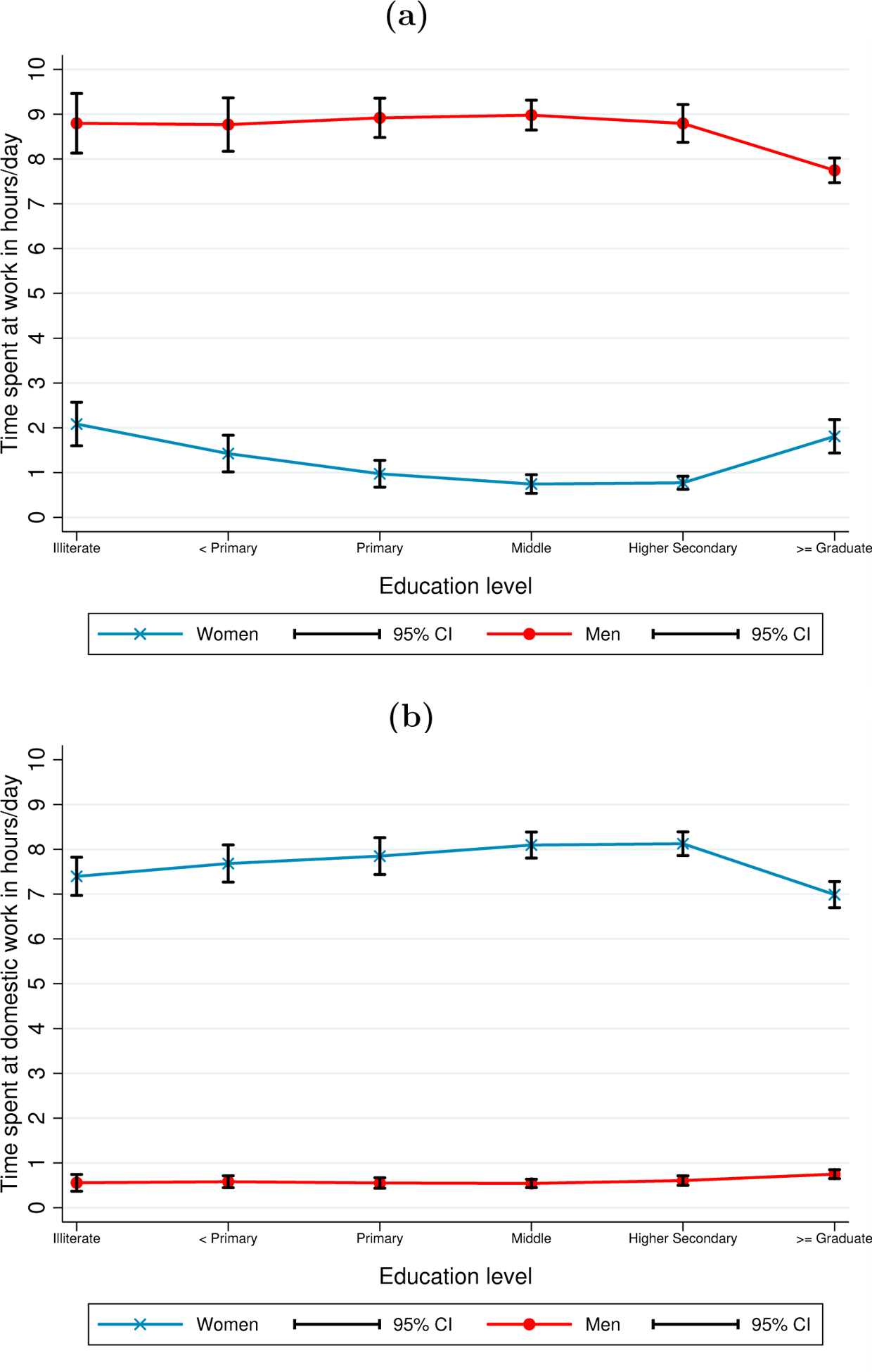
Not surprisingly, Figure 3 shows that average daily hours of work correlate with changes in education as they do at the extensive margin above. More pertinently, we see that the time spent on domestic work is almost the converse of time spent at work for both married men and women (Figure 3), highlighted previously in Afridi et al. (Reference Afridi, Dinkelman and Mahajan2018). Married women spend, on average, 1.33 hours per day in market work and 7.44 hours per day on domestic work (amounting to approximately 10% time being spent on market work by married urban women out of total time spent on all three activities). On the other hand, married men spend almost no time on domestic work (0.6 hours a day) as opposed to 8.36 hours in the labor market. Unconditional on work force participation status, women's time spent on market work decreases monotonically until higher secondary education and then rises marginally for the highest education level—graduate or above. Men spend almost four times more hours in a day on market work.Footnote 15 These pictures reverse when we look at the time spent on home production—increasing monotonically, albeit insignificantly, until highest education level for women and almost flat for men.Footnote 16
Time allocation by education: daily hours (urban, married, age 20–45). (a) Labor supply, (b) domestic work. Source: Time Use Survey 1998 (Authors’ own calculations). Note: Labor supply is calculated by summing up the time spent on labor market activities on the reference day. Domestic work is calculated by summing up the time spent on home production activities on the reference day. The sample size is 3859 and 4389 for men and women, respectively. See data appendix for details of activity classification in the time use data.
From the following section onwards, we focus entirely on the intensive margin of individuals’ time allocation.
2.1 Data
For our analyses we use the two nationally representative datasets discussed above—(1) TUS of 1998 and (2) the NSS, Employment and Unemployment Schedule 1999. In keeping with our previous discussion, the sample is restricted to individuals who are currently married and living in urban areas. We focus on women in the age group of 20–45 years and their husbands in the corresponding age group of 20–60 years.Footnote 17 We generate a dataset where each observation gives the time spent at work (n f and n m), on home production (h f and h m), on leisure (l f and l m), and education levels (i and j) for each married couple along with their weights in the population.Footnote 18 Since educational attainment is not reported in years, we use six different education levels—illiterate, less than primary, Primary, middle, higher secondary, graduate and above. As the TUS does not contain data on wages, the wage returns to education are estimated using the NSS (1999). Corresponding to the sample used in the TUS dataset we restrict the NSS data as well and estimate the median wage for men (w m) and women (w f) corresponding to each education category separately. Our final dataset comprises of 3725 couples (see Appendix B).
Our couples dataset indicates that the average time spent on home production (domestic work) in the household (sum of husband and wife's time) is high, at nearly 8.5 hours per day, equivalent to a full day of market work. There is remarkably little variation in the total home production time by households’ monthly per capita expenditure (MPCE)—8.3 hours for the bottom relative to 8 for the top 10% of MPCE. Of the time spent on domestic work, nearly 1/8th (1.4 hours daily) of this time is spent on exclusive child care, again with barely any variation in child care time across households’ MPCE (Figure A.5 in Appendix A).Footnote 19 This suggests a social benchmark on the time spent on producing the home good of “child quality”—minimum level of human capital of the child.
Additionally, data on households’ education expenditures from the NSS, Consumption Schedule (1999) show that education is one of the largest components of child quality expenditures by households.Footnote 20 Further, we find that child quality, measured by children's learning outcomes, increases with the level of education of their mothers. In the absence of data linking individuals to home-produced goods within the household in the TUS, we utilize the Indian Human Development Survey (IHDS) in 2004–05 to examine the relationship between mother's education and her child's learning. Conditional on a number of confounding factors (viz. household's economic status, father's education, and district of residence), a rise in mother's education is accompanied by higher reading, writing, and math attainment of her children (Table A.1 in Appendix A). This suggests that the productivity of more educated (married) women in home production activities may be higher than that of the less educated.
Based on the above observations, we build a theoretical model that focuses on three determinants of women's labor supply—returns to market, returns to home production, and a social norm represented by benchmarked minimum level of home good.
3 Theory: basics
We construct a variant of the collective decision-making model introduced by Chiappori (Reference Chiappori1988) where time allocation decisions are made at the household level. The model assumes that agents in the economy marry and form a household. Thus, a household consists of two agents, a wife (f) and a husband (m). Henceforth, the terms women/female and men/male will refer to the couple forming the household, i.e., the wife and the husband, respectively.
Individual agents derive utility from private consumption (c), leisure (l), and from a joint home good (H) which is produced and enjoyed by both the members in the household. The total time available to both agents is normalized to one, out of which they allocate time on market work (n), time on producing the home good (h), and leisure (l = 1 − n − h). Agents in the household may also differ in terms of their education level e which is assumed to be finite. While solving the model the education level is assumed to be a continuous variable. Education level of the woman in the household is denoted by i and that of the man by j. In our notation, subscript g ∈ {m, f} is used to represent gender and superscript i or j for education level. Further, we assume that when agents are matched and form a household, both of them derive utility from a common home good H. The utility function of an individual is assumed to be additively separable in its arguments.
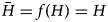
Crucially, following the vast theoretical literature on status building through utility adjustment [see Duesenberry and Press (Reference Duesenberry1949), Clark and Oswald (Reference Clark and Oswald1998), Ljungqvist and Uhlig (Reference Ljungqvist and Uhlig2000), Dupor and Liu (Reference Dupor and Liu2003), Abel (Reference Abel2006), Buraschi and Jiltsov (Reference Buraschi and Jiltsov2007), Barnett et al. (Reference Barnett, Bhattacharya and Bunzel2013), Bishnu (Reference Bishnu2013), among others], we model individual preferences as subject to a benchmark level of home good production. This social norm results in a utility cost that both household members incur if the home good produced is lower than the benchmark specified by society. Thus, while the home good provides utility to both members, the benchmark affects the household adversely. Precisely, unless the family members produce a level of home good H that is more than the social norm $\bar {H}$ , they do not derive any (net) utility from home good production.Footnote 21 We do not put any restriction on the hours worked on women or men on any of their activities directly, hence the social norm is gender neutral. In particular, the form of the utility function is given by,

with g ∈ {m, f}. Parameters ϕ L and ϕ H, both positive, represent the affinity toward leisure and home good, respectively.Footnote 22 Note that the home good (H) varies by education level of the matched couple too but for notational simplicity is represented by H throughout the paper.
We assume that agents’ education is exogenous to household decision-making because it is pre-determined before household formation.Footnote 23 We make the standard assumption that the prevailing market wage rate w is determined by the education level e where w′(e) ≥ 0. Further, we assume that the level of education also determines the productivity (a) of the agents in generating the home good H. In line with the above discussions, the home good H which is produced using a CES technology, is given by,

where h g = h f, h m are the time spent by the woman and the man of the household, respectively, on home production. The terms $a_{f}^{i}h_{f}^{i, j}$ and $a_{m}^{j}h_{m}^{i, j}$
 measure effective time of women and men in production of the home good H, respectively. Further, z g, g ∈ {m, f} represent the share factors in the production function with effective time, where $\sum _{g}{z_{g}} = 1$
 . The parameter ρ > 0 is the inverse of the elasticity of substitution between time spent by the man and woman in the production of the home good. The cost of the market input used in home production is denoted by q. With δ > 0, the model allows for substitution between the agent's time and use of market good available for the production of H. Thus, H measures the effective expenditure in home good production.Footnote 24
Once the agents are matched (married, in our setup) and form a household, they derive joint utility where the Pareto weights of the man and woman are given by θi,j and 1− θi,j , respectively. Pareto weights have a natural interpretation in terms of the relative power of decision-making within the household. These weights are assumed to change with the relative education of spouses. The Pareto weights are, therefore, determined by one's own education [e.g., Thomas (Reference Thomas1994)] and the education of the spouse with whom the agent is matched. The model of collective decision-making allows agents to optimally allocate their time to market work and home production along with leisure, given their relative advantages in market and home production.Footnote 25
3.1 Household optimization
As mentioned above, households solve a joint utility maximization problem by choosing {$c_{f}^{i, j}$ , $c_{m}^{i, j}$
 , $n_{f}^{i, j}$
 , $n_{m}^{i, j}$
 , $h_{f}^{i, j}$
 , $h_{m}^{i, j}$
 , $l_{f}^{i, j}$
 , $l_{m}^{i, j}$
 , q}. Precisely, household's utility maximization problem is given as follows:

subject to,

The first constraint is the income constraint of the household which ensures that the consumption of female and male agents and the expenditure toward market good for home production is equal to the total income of the household. Next, the time availability constraint, which holds for both females and males, guarantees that the total time on the three different activities adds up to one. The third constraint is the technology constraint for the household good production. The last constraint is the usual non-negativity constraint that will hold for both the agents. For notational simplicity, we do not put a superscript or subscript on H but it is denoted for the pair i, j. We introduce the parameter αi,j ∈ (0, 1) which represents the inverse of the responsiveness of home good production to a given social norm.Footnote 26 In our specification, if all households face the same social benchmark $\bar {H}$ , households that produce high H have low αi,j .Footnote 27
The optimization problem defined above guarantees unique interior solutions for the choice variables (see details in Appendix C). The solution to the above problem, using the first-order conditions, is given below:

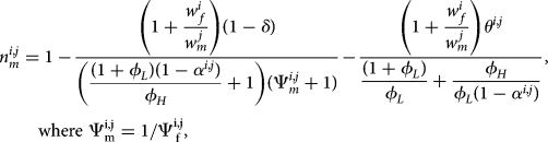


Using the above expressions, it is straightforward to verify that in this proposed theoretical setup, all the endogenous variables are affected by the social norm. More precisely, for a given level of education i, j, if αi,j is low, both members of the household provide lower labor time in home production and the level of leisure increases for both. However, the accompanying change in labor hours provided in the market remains ambiguous. Further, higher norm also results in higher expenditure on market input q required for home good production. The following two relationships are also, then, obvious from above:


Note that while θ affects the ratio of relative market labor supply ($n_f^{i, j}/n_m^{i, j}$ ) as well as leisure ($l_f^{i, j}/l_m^{i, j}$
 ), it does not affect the ratio of time provided for home good production ($h_f^{i, j}/h_m^{i, j}$
 ) because of the public nature of the home good. Also, in this setup relative market labor supply is affected by the benchmark $\bar {H}$
 . This statement follows directly from equations (2) and (3) above. This is a crucial feature of the model, since not only do we want to capture the effect of norm on individual market labor supply (i.e., in absolute terms) but also the variation in the relative labor supply with the benchmark level of $\bar {H}$
 . This implies that the norm affects the market labor supply of both agents, however the effects are not symmetric and therefore the relative market labor supply is not independent of the parameter αi,j .
3.1.1 Theoretical decomposition of effects
The following expression for the allocation of time to market work by a wife with education level i and husband's education level, j, is obtained in this model,

where $\Psi _{f}^{i, j} = ( {z_{m}\over z_{f}}) ^{1/\rho }( {w_{f}^{i}a_{m}^{j}\over w_{m}^{j} a_{f}^{i}}) ^{{1-\rho \over \rho }}$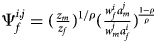 .
Note that Ψf falls with the relative home productivity ratio a f/a m but increases with the wage ratio w f/w m. Given that, the following three observations are clear from the above expression of $n_{f}^{i, j}$ . First, keeping other factors constant, $n_{f}^{i, j}$
 increases with the level of w f/w m, that is, a relative wage that favors women encourages FLFP. Second, $n_{f}^{i, j}$
 decreases with the Pareto weight on men (1 − θi,j ), ceteris paribus. This implies that the higher the bargaining power of women in household decision-making, the lower is the supply of market work by them (at the same time, they enjoy more consumption and leisure).Footnote 28
Third, $n_{f}^{i, j}$ decreases with the level of home productivity ratio a f/a m. As the home productivity of women relative to men increases, the supply of market work by women falls, holding other factors constant. Each of these three effects is for a given level of αi,j . As we have mentioned above, the effect of αi,j on $n_{f}^{i, j}$
 is ambiguous.
To understand how the labor supply of a wife at an education level i + 1, matched with a husband of education level k, is different from that chosen by a wife with a lower education level i, matched with a husband of education level j, we can take the difference between $n_{f}^{i + 1, k}-n_{f}^{i, j}$ which can be written as,

Equation (7) shows that the difference in the allocation of time to market work by a wife as her education level increases can be explained using the three components shown in the under-brackets. We first discuss the role of the three components, keeping αi,j constant across education levels. The first component (a) is clearly the effect of a change in Pareto weights when the wife's education increases (now matched to a husband having a different education level). The second component (b) reflects a combined effect of the Pareto weights and relative female wage. The third component (c) reflects the combined effect of relative female wage and relative female home productivity. All three factors in these components—Pareto weights, relative female wage, and relative female home productivity—vary with the education level for a fixed α. The next paragraph sheds some light on the sign of the expression $n_{f}^{i + 1, k}-n_{f}^{i, j}$ .
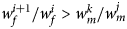
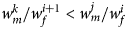
The effect of a change in Pareto weights through (a) on the marginal labor supply is straight forward: higher Pareto weights for women imply less time allocated by them in market work. To understand term (b) better, let us first assume that Pareto weights are invariant to education and equal 1 − θ. Then (b) can be written as $( 1-\theta ) ( {w_{m}^{j}\over w_{f}^{i}}-{w_{m}^{k}\over w_{f}^{i + 1}})$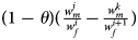 which says that if the relative wage in the higher education category is greater than the relative wage in the previous education group, that is if $w_{m}^{k}/w_{f}^{i + 1}< w_{m}^{j}/{w_{f}^{i}}$
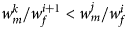 [or equivalently if $w_{f}^{i + 1}/{w_{f}^{i}}> w_{m}^{k}/w_{m}^{j}$
 , i.e., the relative gain in wage by a more educated woman is higher than the relative gain (or loss) in male wage], then this will increase the wife's labor supply. Thus, women's labor supply to market work will depend positively on a favorable movement of the gender wage ratio toward them. This inequality may not hold if (1 − θ) varies with education since $w_{m}^{k}/w_{f}^{i + 1}< w_{m}^{j}/{w_{f}^{i}}$
 does not necessarily imply $( 1-\theta ^{i + 1, k}) w_{m}^{k}/w_{f}^{i + 1}< ( 1-\theta ^{i, j}) w_{m}^{j}/{w_{f}^{i}}$
 . To understand the term (c), we first assume that the home productivity ratios are constant, that is, ${a_{m}}/{a_{f}} = {a_{m}^{j}}/{a_{f}^{i}} = {a_{m}^{k}}/{a_{f}^{i + 1}}$
 . Given that, a favorable wage movement, which means an improvement in the relative female wage in a higher education category, guarantees an increase in her labor supply. However, in our model home productivity varies with education. Hence as the gender ratio of home productivity improves in favor of the wife with her education level, the wife's labor supply may fall due to (c).
Briefly, when all the three factors are allowed to vary, the final effect of a change in education on labor supply depends on the direction and relative magnitudes of the movements in (a), (b), and (c). While the previous literature has focused on the role of gender wage ratio and Pareto weights, our model shows that varying home productivity with the level of one's education is important for this analysis. The above discussion clearly shows that the model is capable of generating both a rise and a fall in market labor supply (U-shape) of married women as their education increases. For instance, for women with higher levels of education who may have a favorable gender wage ratio, this model can generate little increase (or in fact a fall) in market work if the rise in the home productivity ratio is much larger than the rise in wage ratio at that education level.
The discussion above is for a fixed level of αi,j and αi+1,k. However, note that H is a normal good with respect to household (total) income and therefore with an increase in the level of education (hence wages), the level of home good production increases. Since in our theoretical model we assume a universal social norm $\bar {H}$ that is constant across all education groups, given the multiplicative relationship between H and $\bar {H}$
 (section 3.1 above), α is lower for the education group that produces a higher level of home good H. Thus a fall in α with increase in education reduces the market labor supply of the wife through the components (a) and (b). However, a fall in α through the component (c) results in an increase in her market labor supply. This means that keeping all else constant, when relative home productivity and its interaction with the relative market wage is taken into consideration, a decrease in α augments the market labor supply of the wife. Thus, the overall effect of a change in α due to a higher level of education of the wife suitably matched with a husband can be of either sign depending on the characteristics of the economy.Footnote 29
Table 1 summarizes the theoretical predictions in the movement of the four factors in equation (7)—relative wages (column 2), relative home productivity (column 3), relative Pareto weights on men (column 4), and relative change in responsiveness to social norms on home production (column 5)—on changes in wife's labor supply. Row 1, columns (2)–(4) show the effect on wife's labor supply for each factor when these factors increase across education levels, i.e., the direction of change in them is > 1. For instance, following the above discussion, a relative increase in female to male wage ratio as wife's education level increases, leads to an increase in wife's labor supply across education levels (denoted by > 0 in column 2, row 1). Row 2 shows the predicted effect when these factors decrease across education levels, i.e., the direction of change in them is < 1. For instance, in row 2, a relative decrease in female to male wage ratio as wife's education level increases, decreases wife's labor supply across education levels (denoted by < 0 in column 2, row 2). The effects of change in home productivity, Pareto weights, and norm responsiveness on wife's labor supply can be read in similar manner following the discussion above.Footnote 30 The last row shows that in the trivial case when none of the four factors change with wife's education (= 1), there is no change in her labor supply.
Theoretical predictions of effects on wife's labor supply
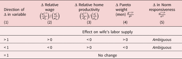
Note: Column 1 shows the direction of change in each of these four variables—relative wages (column 2), home productivity (column 3), Pareto weight (column 4), and norm responsiveness (column 5). Each cell in columns 2–5 shows the predicted direction of change in wife's labor supply for a given change in the corresponding variable (column 1) when her education increases. The predictions follow the theoretical decomposition of changes in wife's labor supply derived from equation (7). For example, an increase (> 1, depicted in row 1 in column 1) in the relative wage ratio when wife's education level increases, raises her labor supply (> 0, row 1 in column 2).
We now turn to calibrating and simulating our model on agents’ time allocation to market work, home production, and leisure.
4 Calibration and simulation
4.1 Calibration
The Pareto weights for each of the 36 combinations of spousal education are calibrated using the ratio of the first-order conditions. We have no a priori reason to assume that men and women have the same bargaining power within the household (θ = 0.5), and across education categories. Utilizing equation (6) from the model which relates the leisure ratio of men and women to θi,j and their wages, we have:

From the TUS couples data, we substitute for average values of time spent on leisure by a woman and a man, and for median wages received by a woman and a man, for each combination of education categories of spouses. This gives us 36 values of θs for each possible combination of spouses with different education levels.Footnote 31
Next, we discuss the calibration of the (inverse of) responsiveness to the social norm—the ratio of the benchmarked minimum home production to actual home production—for each spousal education group ($\alpha ^{i, j} = {\bar {H}\over H^{i, j}}$ ). As discussed earlier, the home production function in our setup measures the effective expenditure on the home good (expenditure adjusted for home productivity).Footnote 32 We use data on average household education expenditure per child in urban India [from NSS (1999)] as a proxy for effective expenditure on home good production.Footnote 33 We then compute the extent to which each education group exceeds the norm on home good production, i.e., the ratio of the minimum expenditure on education per child that must be incurred ($\bar {H}$
 ) to the actual education expenditure per child incurred by an education group (H). The first percentile value of education expenditure per child of the lowest spousal education group (e f = Illiterate and e m = Illiterate) denotes the benchmarked minimum level of home good production that must be incurred by all education groups, i.e., $\bar {H}$
 . We assume this minimum education expenditure, $\bar {H}$
 , to be fixed across all spousal education categories while the average household expenditure on education per child for each combination of spousal education (H) varies across spousal education groups. Using this procedure, we are able to calibrate the value of α for each of the 36 education groups.
The parameters of the home production function—home productivity ($a_{f}^{i}$ , $a_{m}^{j}$
 ) and share of female and male labor input into home production (z f, z m)—and the preference parameters (ϕ L and ϕ H) are estimated using the closed form solutions obtained in the model. The observed values of each couple's time spent in the market and in home production are fitted to the theoretical expressions in equations (2), (3), (4), and (5). This method gives the estimates for the 12 home productivity parameters (six each for men and women corresponding to each of the six education categories) and the three parameters—z m, ϕ L, and ϕ H—which do not change across education categories. We are able to obtain a set of unique solutions for all the calibrated parameters using non-linear least squares.Footnote 34
The calibrated parameters are shown in Table 2. For simplicity, the 36 calibrated Pareto weights (for each possible i, j education combination of wife and husband) are averaged for each education group of women in the table. The average household Pareto weight on wife's utility does not change significantly across lower education categories (on average it is 0.27 for illiterate—middle education women) but it increases drastically for women with more than higher secondary education (approximately 0.45). The change in bargaining power with wife's education is, therefore, unlikely to explain the initial decline in female LFPR and may reduce women's LFPR only at higher secondary education or above.
Calibrated parameters
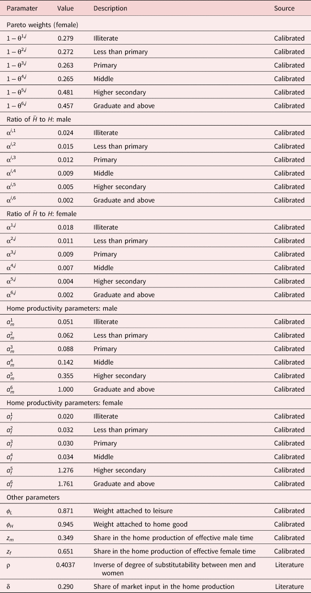
Note: To ease presentation the 36 calibrated Pareto weights and α values (for each possible i, j education combination of wife and husband) are averaged for each education group of women and men in this table.
As expected, α decreases as education increases since more educated women (men) produce a higher value of the home good (child quality) relative to the benchmarked minimum—in line with the theoretical analysis above. Thus α decreases from 0.018 (0.024) for illiterate women (men) to almost 0.008 (0.010) for primary-middle educated women (men) and further to 0.003 (0.002) for higher secondary and above educated women (men). Hence, on average women (men) in the highest education group produce almost 9 (12) times as much of the home good as illiterate women (men).
The estimated home productivity parameters show that home productivity increases with increase in education for both men and women, with the rate of increase being largest for the highest education categories. The increase is smaller and uneven, though, for lower levels of education. Across the disaggregated education levels, from less than primary to middle schooling, home productivity is very similar. It would then be more intuitive to look at the comparison across broad four categories of education—illiterate, women with some education (less than primary—middle classes), completed schooling, and graduate. Here, we do find an unambiguous increase in home productivity between illiterate women (0.02) and women with some education (0.034) by almost 70%.
The share parameters in the home production function show that men's effective time spent in home production is about 35% and that by women is 65%. Though, on an average women's share of overall time in home production is almost 90%, adjusted for home productivity this falls to 65%. This could be driven by a higher average home productivity of men relative to women up to middle education levels, as shown in the panel above of Table 2. We also find that the ratio of ϕ H and ϕ L is 1.1, indicating that households place a greater weight on home production than leisure. Two behavioral parameter values are borrowed from the literature for the US—(1) the inverse of the elasticity of substitution, ρ is set at 0.4037 and (2) δ, which measures the relative share of market inputs to labor in home production is set at 0.29.Footnote 35 Later we conduct sensitivity analyses to show that using different values of ρ or δ don't change the results significantly.
To summarize, our calibration results approximate the broad patterns observed in the Indian economy and also capture the household preferences in time allocation.
4.2 Simulation
In this section, we first verify the contribution of each channel toward the observed movements in wife's labor market time. To do this, we use data on wages and the calibrated parameters to calculate the movement of relative wages, home productivity, Pareto weights, and the (inverse of) responsiveness to the social norm (i.e., the extent to which the benchmarked minimum home production is lower than actual home production) across education levels. These are reported in Table 3 for changes across each consecutive education level in column (1), denoted by the following numeric codes: 0 − illiterate, 1 − less than primary, 2 − primary, 3 − middle, 4 − higher secondary, 5 − graduate and above.
Estimated changes in factors affecting wife's time allocation

Source: Time Use Data and NSS. Note: Numeric education codes denote the following education levels. 0 − Illiterate, 1 − less than primary, 2 − primary, 3 − middle, 4 − higher secondary, 5 − graduate and above. Average relative wage, relative home productivity, Pareto weight, and norm responsiveness is estimated for each level of wife's education using the calibrated parameter values from time use data for 3725 couples. Changes in estimated ratios across successive education levels are reported in columns 2–5.
It can be seen that the relative female wage ratio in column (2) of Table 3 declines (or increases by less than one) for each consecutive level between illiterate and middle schooling. This observed fall in relative female wages contributes toward reducing wife's labor supply with an increase in her education up to middle schooling. Thereafter, the relative female wage ratio increases (or change by more than one) for education levels from middle—graduate and above, which would raise wife's labor supply between these education levels. These findings are in line with the theoretical predictions in Table 1, column (2), which shows that wife's relative labor supply is positively related with relative female wages. Similarly, an increase in relative female home productivity from illiterate to less than primary and middle to higher secondary [denoted by a change of more than one in column (3) of Table 3 for these education levels] would contribute toward reducing female labor supply across these education levels [Table 1, column (3)]. Column (4) shows that bargaining power of men does not change much when wife's education increases from illiterate to middle schooling while it falls when wife's education increases from middle to higher secondary schooling. As predicted in Table 1, column (4), this should contribute towarddecreasing the wife's labor supply from middle to higher secondary schooling, holding other factors constant. Lastly, column (5) shows that α decreases across successive levels of wife's education, which has an ambiguous effect on wife's labor supply, as discussed theoretically earlier.
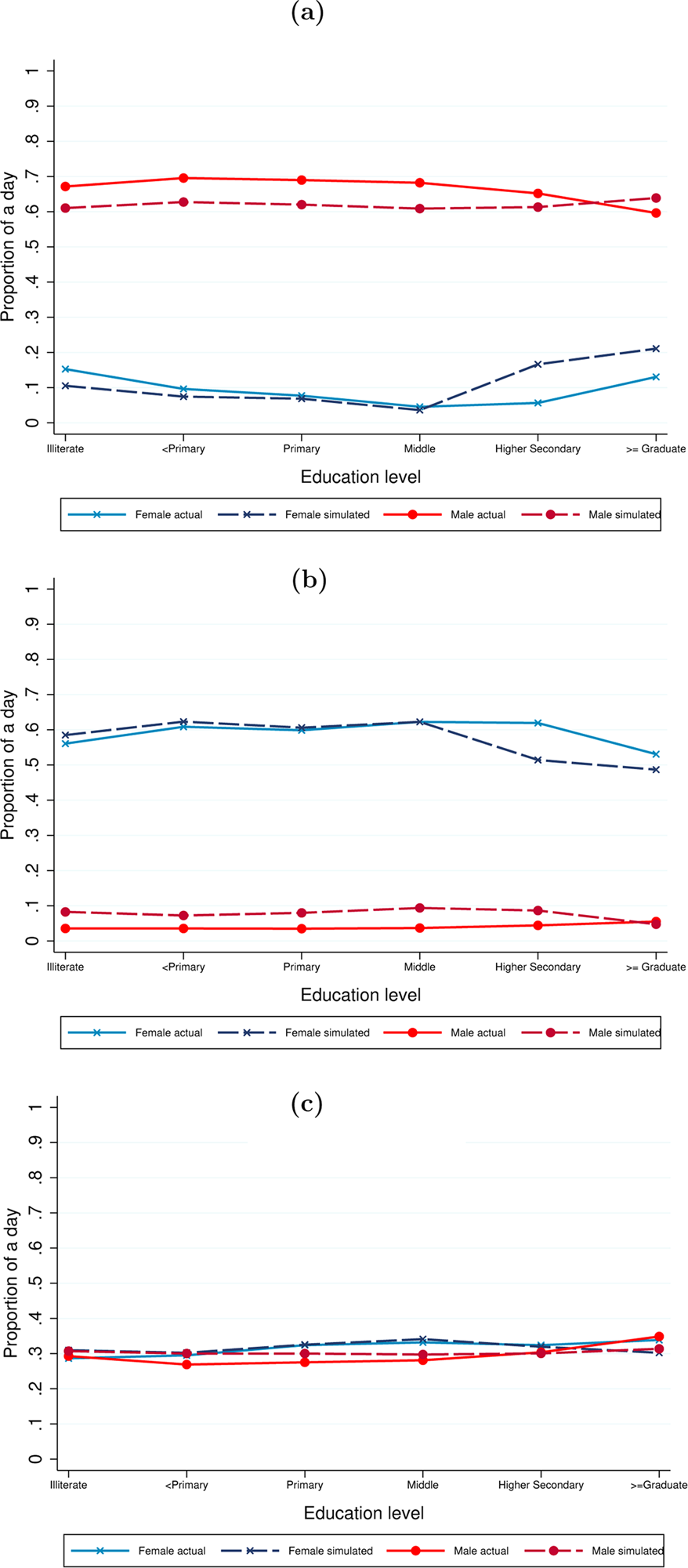
Using the estimated wages and the calibrated parameters we predict the time spent in the labor market, home production, and leisure for individuals in each education group in urban India, accounting for all the four factors simultaneously. Figure 4 plots the model's predictions against the actual time allocations observed in the data for women and men by education groups. The model is successful in generating a U-shaped female labor supply with respect to their education level—women's time allocation to market work falls from 11% for the illiterate to 7% for those with less than primary or primary levels of schooling and further to 4% at middle education level. It then rises to 17% and 21% for the two highest education levels, respectively. For men, the simulations mimic the relatively stable allocation of time to market work at over 60% across the education groups, though it somewhat under predicts market work at lower education levels. Overall the model does well for the time allocation variables that we are focusing on in this analysis, including the large gender gap in time devoted to home good production.
Simulations for time spent in labor market, home production, leisure. (a) Labor supply, (b) domestic work, (c) leisure. Note: Time spent in labor market, home production, and leisure is shown as a fraction of the total time endowment of one. See data appendix for details on time use data.
5 Discussion
In previous sections we constructed a theoretical model with changing market productivity, home productivity, and a norm on home good production. Using the TUS datasets for India we now calibrate and simulate the standard model—which allows only market productivity to vary across education groups (i.e., home productivity is constant and there is no additional utility from generating more home good than a basic minimum benchmark)—for comparison with our analysis.Footnote 36 We allow bargaining power to vary with education in both models.
Table 4 shows the allocation of time to work, home production, and leisure, predicted at each education level, in the data (column 1) standard model (column 2) and the model posited in this paper (column 3) for women (panel A) and men (panel B). In panel A varying market productivity and keeping home productivity constant (column 2) predicts a U-shaped relationship between women's education and market work but it does not reproduce the fall in labor supply from illiterate to less than primary education levels. The standard model also predicts 19–23 percentage points higher time allocation to market work for the two most educated groups of women—those having higher secondary education and those who are graduate and above. Moreover, it under predicts time spent in home production by women at all education levels but by much more at the highest education levels—24–32 percentage points—as shown in column (2) relative to column (3) in the middle panel. The time allocated to leisure by women reported in the bottom panel of Table 4 is consequently over predicted by the standard model across the education distribution, again more so for the two highest education levels when we compare columns (2) and (3). For men, the standard model somewhat under predicts their labor supply and overpredicts leisure (Table 4, panel B).
Comparison across models

Note: Column (1) shows the actual value of time spent in a particular activity. Column (2) shows the predicted time spent in an activity obtained by calibrating a model where home productivity is constant across education levels and there is no social norm imposed on home produced good. Column (3) shows the predicted time spent in an activity obtained by calibrating a model where home productivity varies across education levels and there is a social norm imposed on the amount of home good produced. Panel A shows these for women while panel B shows these for men.
In contrast, the model posited in this paper performs much better than the standard model as shown in column (3) of Table 4. First, it reproduces the fall in women's labor supply from illiterate to less than primary education levels and second, the gap between the predicted and actual labor supply for women with higher secondary and graduate or above education falls to 11 and 8 percentage points, respectively, relative to the standard model. The predicted time spent in home production by women increases and now matches closely with the actual time spent in domestic work. The match is almost perfect for lower education groups although we still under predict time spent in home production by women for the highest education group. Consequently, predicted time allocated to leisure by women in the bottom of panel A, Table 4 is lower and closer to the actual data, for the model posited in this paper as shown in column (3).
To summarize, the fall in relative female wage between illiterate to middle schooling combined with an increase in relative female home productivity between illiterate to less than primary explains the fall in wife's labor market time upto middle education levels. Thereafter, between middle to graduate and above education levels, the muted increase in female labor time is explained by a large increase in relative female home productivity and bargaining power within the household between these education levels. These findings are in line with the theoretical expositions discussed in Table 1, which show that relative female labor supply increases with a rise in relative female wage but decreases with increase in relative home productivity and relative female bargaining power. Further, social norms on a benchmark level of home good production play a role in explaining the low levels of women's time allocation to market work. Our model performs better than the standard model since it incorporates all the four channels—changes in relative wage, home productivity, bargaining power, and social norms toward home good production.
The model is able to explain the low and stagnant level of women's labor supply for the lower education groups and to a large extent, though not fully, for women having more than secondary education in India. Even after accounting for the supply side factors, an 8 percentage point gap remains between the predictions of our model and the actual labor supply of women who have graduate or higher education. This could possibly be explained by the low level of demand for women's labor or differences in the type of work demanded by women (for instance, flexible time schedule) and those available in the market at higher levels of education in India [Afridi et al. (Reference Afridi, Dinkelman and Mahajan2018)].
6 Alternative mechanisms
In this section we test for and reject alternative mechanisms that can explain the time allocation decisions of households, particularly for women at higher education levels.
6.1 Market goods for home production
In low or middle-income countries, limited supply of market goods can constrain women's time allocated to market work. This may be especially true for the more educated women, who are also more likely to belong to higher income households, and can afford to purchase market goods for home production. Hence the lack of or limited supply of market goods and services could be an alternative explanation of both low levels of women's time allocated to labor market and the muted response of women at higher levels of education to market wages.
Note that in our setup, households choose optimal amount of market good in home production. To test for the possible mechanism described above we constrain the usage of market goods in the model by imposing a restriction that q is same across education levels and that $q \leq \bar {q}$ . Here $\bar {q}$
 is defined to be strictly less than the minimum of the optimal q obtained across all education levels in the main model. This modification reduces wife's labor supply at higher education levels, in comparison to our model, but by a negligible amount. Since in our original setup q is chosen optimally, households respond to a constant amount of q (which is also lower relative to the optimal) by reducing the total H produced at higher education levels, while H still exceeds the minimum benchmark of $\bar {H}$
 for high education groups. Thus, even though the total H produced by the household rises with education, the level of H is now lower due to the constraint on the market good. Hence, instead of increasing time spent on home production by the wife and consequently reducing her labor supply, restricting q primarily results in lower production of the home produced good. Thus, the absence or low supply of market goods may not explain the observed levels of women's time spent on market work in India.Footnote 37
6.2 Household wealth
Another possible channel that could impact women's labor supply is household wealth. As female education levels increase, households are more likely to be wealthier, inducing a wealth effect which could lower women's LFP. We, therefore, incorporate exogenous increases in household wealth over the distribution of education using the 2003 National Sample Survey on Household Assets (NSS-HA) which collected information on assets owned by households. Appendix Figure A.6 plots the simulations for labor supply, domestic work, and leisure after incorporating the wealth effect. We do observe some reduction in labor supply but not substantially over and above our model's predictions. Overall, the estimated household wealth from land or residential property is too small to predict the muted allocation of time to market work by highly educated women.Footnote 38
7 Robustness checks
7.1 Sensitivity analyses
We conduct sensitivity analyses of the predicted paths of labor supply, home production, and leisure for the parameters which could not be calibrated and were taken from the existing literature on the US—the inverse of the degree of substitutability between men and women (ρ) and the share of market inputs in home production (δ). Under the assumption that men and women are imperfect substitutes in home production (i.e., 0 < ρ ≤ 1), we calibrate our model taking different values of ρ ∈ [0.2, 0.6] around the benchmark value of 0.4037 in the literature.Footnote 39 The predicted paths do not change much because the share of men's time in home production is smaller than women's. Similarly, we calibrate the model with δ ∈ (0, 0.29). The benchmark value of δ taken from the US data is 0.29 (an average across various studies). The calibrated value of δ for the US depends on whether housing is included as a market good or not. In the Indian context, since the share of market goods is likely to be smaller than that for a developed country, for sensitivity checks we take values less than 0.29. The predicted paths again do not change much. The results for these sensitivity checks are available on request.
7.2 Variation of social norm across education groups
Recall that our theoretical model assumes a single $\bar {H}$ for society, i.e., the minimum benchmark for the home good is the same for all education groups. However, it is possible that $\bar {H}$
 varies by education—higher education groups may desire higher minimum level of child quality. Notably, we calibrate the value of α, which represents the ratio of $\bar {H}$
 , to actual H. When higher education groups have a higher benchmarked level of home good, the ratio of the two (${\bar {H}\over H}$
 ) may not vary significantly across education groups, since they also produce higher levels of H.Footnote 40
We check the robustness of our results to calibrating α using the first percentile value of education expenditure per child for each education group as the $\bar {H}$ for that group. Indeed, Appendix Table A.2 shows that α does not vary much across education of women and men, except for the highest education group, when we allow $\bar {H}$
 to vary by education groups. Appendix Figure A.7 plots the simulations for labor supply, domestic work, and leisure using this alternative model. We do not find much difference from our previous predictions when $\bar {H}$
 is constant across education groups.Footnote 41
7.3 Recent employment data
We conduct our analysis by approximating individuals’ time allocations using the most recent, comparable employment data from the NSS 2011. The details of our assumptions for the approximation of time-allocation and the simulation results using the NSS 2011 are discussed in Appendix A and Figure A.8. Specifically, Appendix Figure A.9 shows that the labor supply simulation results for our model predicts well the U-shaped labor supply of women across education categories in 2011 as well.
8 Conclusion
Low and stagnant allocation of time to the labor market by women in India despite economic growth and higher educational attainment is a puzzle. While the decline in the gender gap in education is often accompanied by a more favorable gender wage ratio at higher levels of education, women exhibit little responsiveness in terms of increasing their labor market attachment. In this paper we develop a model that is capable of generating these observed regularities in women's labor supply by their education level. We use detailed individual time use data for urban India to show that a rise in home productivity with education along with a social norm on producing a minimum benchmarked level of the home good can explain the U-shaped relationship between married women's time allocation and their education. Importantly, the assumed social norm is not imposed on any particular gender, but rather on the entire household, therefore, our results are driven by differential home and market productivity of household members.
Our model predicts the observed patterns in the data more closely than a standard model with home production but without home productivity and social norms. The analysis, thus, contributes to the existing literature on women's labor supply, broadly, and to the ongoing debate on women's LFP in developing economies such as India. We show that multiple factors, and their interplay, can explain the persistent gender gap in LFP and the non-monotonic relationship between women's market labor supply and their education.
While we do not incorporate demand side factors affecting women's LFP explicitly, to the extent that labor demand is reflected in the equilibrium market wage, they are accounted for in the analysis. Nevertheless, it is possible that differences between the type of work demanded by women and those available in the market constrain their employment opportunities at higher education levels. Thus demand-side factors may account for the residual gap between women's predicted and observed time spent on market work in our analysis.
Supplementary material
The supplementary material for this article can be found at https://doi.org/10.1017/dem.2022.22.
Acknowledgments
The authors thank the editor and two anonymous referees for their feedback. Orazio Attanasio, Jere Behrman, Shankha Chakraborty, Seema Jayachandran, Alok Johri, David Lam, Rohini Pande, Christian Siegel, Morten Ravn, and participants at the ACGDE conference (ISI, Delhi), Women in the Economy workshop (ISI, Delhi), Economic Development in South Asia conference (CDES, Monash University), IZA/World Bank/NJD conference on Jobs and Development (Washington DC) and IUSSP conference on Population, Poverty and Inequality (Ann Arbor) provided useful insights. Bishakha Barman and Nitesh Yadav provided exceptional research assistance. Afridi acknowledges financial support from IWWAGE-IFMR, a Bill and Melinda Gates Foundation initiative.
Financial support
This study was funded by IWWAGE-IFMR (a Bill and Melinda Gates Foundation Initiative) through a sub-award to the Indian Statistical Institute, Delhi.
Conflict of interest
None.