1 Introduction
This paper provides a numerical analysis of the energy exchanges associated with the half-trace of the velocity fluctuation correlation tensor in a low Mach turbulent channel flow subjected to a strong temperature gradient. The investigation is relevant to the study of wall-bounded turbulent flows with variable fluid properties, provided that acoustic effects are small. Flows subjected to a large temperature gradient are characterized by a strong coupling between temperature and turbulence (Serra, Toutant & Bataille Reference Serra, Toutant and Bataille2012a ; Toutant & Bataille Reference Toutant and Bataille2013). The statistics of velocity and temperature means and fluctuations are modified by the temperature gradient, as an asymmetry between the turbulence statistics at both walls is generated. This asymmetry is more complex than a Reynolds number effect, as the scaled statistics of turbulence do not collapse with those of the isothermal channels at the turbulence Reynolds number corresponding to either wall of the anisothermal channel (Serra et al. Reference Serra, Toutant, Bataille and Zhou2012b ). The energy exchanges between the different parts of total energy are insightful for the fundamental understanding of the behaviour of flows subjected to a strong temperature gradient. They include in particular the energy exchanges associated with turbulence kinetic energy. The use of flow fields from direct numerical simulations has demonstrated its relevance to the investigation of energy exchanges. Indeed, this requires the knowledge of the instantaneous three-dimensional velocity, pressure and temperature fields, which cannot be easily obtained experimentally.
In incompressible flows with constant fluid properties, direct numerical simulations of homogeneous isotropic turbulence have validated Kolmogorov’s hypothesis on the locality of the energy transfer (Domaradzki & Rogallo Reference Domaradzki and Rogallo1990) and interacting scales (Zhou Reference Zhou1993a ,Reference Zhou b ). Reliable statistics of the terms of the evolution equation of the turbulence kinetic energy in a channel flow have been provided in the spatial domain by various authors, including Kim, Moin & Moser (Reference Kim, Moin and Moser1987), Moser, Kim & Mansour (Reference Moser, Kim and Mansour1999), Abe, Kawamura & Matsuo (Reference Abe, Kawamura and Matsuo2001), del Álamo & Jiménez (Reference del Álamo and Jiménez2003), Hoyas & Jiménez (Reference Hoyas and Jiménez2006), Kozuka, Seki & Kawamura (Reference Kozuka, Seki and Kawamura2009) and more recently Vreman & Kuerten (Reference Vreman and Kuerten2014). The analysis of the energy transfer processes in the incompressible channel flow has been pursued in the space of scales through the analysis of the second-order structure function by Marati, Casciola & Piva (Reference Marati, Casciola and Piva2004), Cimarelli, De Angelis & Casciola (Reference Cimarelli, De Angelis and Casciola2013), Cimarelli & De Angelis (Reference Cimarelli and De Angelis2014), Cimarelli et al. (Reference Cimarelli, De Angelis, Schlatter, Brethouwer, Talamelli and Casciola2015, Reference Cimarelli, De Angelis, Jiménez and Casciola2016) and in the spectral domain by Domaradzki et al. (Reference Domaradzki, Liu, Hartel and Kleiser1994), Bolotnov et al. (Reference Bolotnov, Lahey, Drew, Jansen and Oberai2010). In compressible flows with highly variable fluid properties, the turbulence kinetic energy may be defined in several manners according to the chosen decomposition of total energy. The main approaches are the density-weighted averaging decomposition (Favre Reference Favre1965), the mixed-weighted decomposition (Bauer, Zumwalt & Fila Reference Bauer, Zumwalt and Fila1968), the density square-root-weighted decomposition (Yih Reference Yih1960) and the classical averaging decomposition (Chassaing Reference Chassaing1985). The reader may find more details on these decompositions in Cousteix & Aupoix (Reference Cousteix and Aupoix1989), Aupoix (Reference Aupoix2000), Chassaing et al. (Reference Chassaing, Antonia, Anselmet, Joly and Sarkar2013), Gatski & Bonnet (Reference Gatski and Bonnet2013). Numerical analyses of the turbulence energetic behaviour may be carried out using any of the above-mentioned definitions of turbulence kinetic energy. Notable works include Ha Minh, Launder & MacInnes (Reference Ha Minh, Launder and MacInnes1982) for the mixed-weighted decomposition and Kida & Orszag (Reference Kida and Orszag1992), Cook & Zhou (Reference Cook and Zhou2002) for the density square-root weighted decomposition. To the knowledge of the authors, there is no such reference numerical analysis based on the classical averaging decomposition. By contrast, the density-weighted averaging decomposition has been used by many authors. In particular, the energy exchanges associated with turbulence kinetic energy in compressible channel flows with a high Mach number have been investigated extensively (Huang, Coleman & Bradshaw Reference Huang, Coleman and Bradshaw1995; Guarini et al. Reference Guarini, Moser, Shariff and Wray2000; Maeder, Adams & Kleiser Reference Maeder, Adams and Kleiser2001; Lechner, Sesterhenn & Friedrich Reference Lechner, Sesterhenn and Friedrich2001; Pirozzoli, Grasso & Gatski Reference Pirozzoli, Grasso and Gatski2004; Shahab et al. Reference Shahab, Lehnasch, Gatski and Comte2011; Shadloo, Hadjadj & Hussain Reference Shadloo, Hadjadj and Hussain2015). The density-weighted averaging is indeed well suited to the physics of compressible flows. The low Mach channel flow subjected to a strong temperature gradient has received less attention from the literature. The sole analysis has been carried out in the spectral domain with the density square-root-weighted decomposition by Aulery et al. (Reference Aulery, Toutant, Bataille and Zhou2015, Reference Aulery, Dupuy, Toutant, Bataille and Zhou2017) at a mean friction Reynolds number of 180 and 395. The two studies use a decomposition of the terms of the evolution equation of turbulence kinetic energy based on the work of Bolotnov et al. (Reference Bolotnov, Lahey, Drew, Jansen and Oberai2010). The literature thus lacks a detailed study of the effect of the temperature gradient on the spatial profiles of the energy exchanges associated with turbulence kinetic energy.
Thereupon, this paper analyses the energy exchanges associated with the half-trace of the velocity fluctuation correlation tensor using a decomposition of turbulence kinetic energy based on the classical averaging. One of the main advantages of the classical averaging is that it is the usual way to extend the study into the spectral domain. Within the formulation used, each term of the evolution equation of the half-trace of the velocity fluctuation correlation tensor is associated with an energy exchange. In that sense, each term is given a physical meaning. Each term is then decomposed in the particular case of a fully developed channel flow to isolate the parts that are formally identical to the terms remaining in flows with constant fluid properties, and the terms specific to flows with variable fluid properties. These terms are related to the flow dilatation, the variation or the fluctuation of the fluid properties or the presence of a mean wall-normal velocity. The decomposition is carried out in both the spatial and spectral domains. There is a one-to-one correspondence between the terms of the spatial and spectral decompositions.
In this paper, we use this property to investigate the energy exchanges associated with the half-trace of the velocity fluctuation correlation tensor in the spatial and spectral domains in a consistent manner. This ensures that the integration of the spectral term is exactly equal to the associated spatial term. To compute the terms, we carry out two direct numerical simulations of a fully developed low Mach turbulent channel flow: one isothermal and one anisothermal. In both cases, the mean friction Reynolds number of the simulation is 180. The effects of gravity are neglected. In the anisothermal simulation, the temperatures of the two channel walls are 293 K and 586 K. Compared to the isothermal simulation, the only new physical phenomenon is the variations of density, viscosity and conductivity with temperature. The numerical set-up is validated in the isothermal configuration with the data of Moser et al. (Reference Moser, Kim and Mansour1999), Bolotnov et al. (Reference Bolotnov, Lahey, Drew, Jansen and Oberai2010) and Vreman & Kuerten (Reference Vreman and Kuerten2014). The spatial and spectral amplitudes of each term are assessed. This allows us to determine the relative importance of each term, and in particular evaluate the importance of the terms specific to flows with variable fluid properties. Then, we study the effect of the temperature gradient on the energy exchanges. In the spatial domain, the results extend the existing literature in the isothermal configuration to the anisothermal configuration. In the spectral domain, the analysis provides new insights into the spectral energy exchanges in both the isothermal and anisothermal configurations, since the energy exchanges have not been studied with the same decomposition in the incompressible literature.
The ternary representation of the energy exchanges used in this paper is summarized in § 2. The detailed channel flow configuration, the numerical set-up and the data acquisition are presented in § 3. The results are discussed and analysed in § 4.
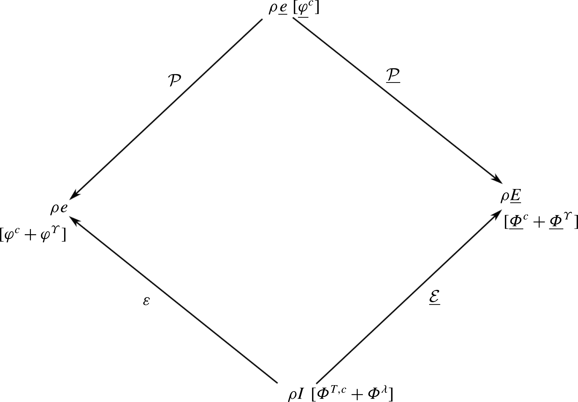
Schematic representation of the energy exchanges between the four parts of total kinetic energy in the ternary representation. An arrow represents an interaction between two quantities.

2 Energy exchanges associated with the half-trace of the velocity fluctuation correlation tensor in the ternary decomposition
The ternary representation of the energy exchanges is based on the decomposition of velocity into a mean and fluctuating part with the classical (non-density-weighted) averaging (Reynolds Reference Reynolds1894). Let us denote (
 $\overline{\phantom{ia}}$
) the statistical average operator and (
 $^{\prime }$
) the fluctuating part operator. The velocity is decomposed as
 $U_{i}=\overline{U}_{i}+u_{i}^{\prime }$
, where
 $U_{i}$
the
 $i$
th component of the velocity. We use a lowercase
 $u^{\prime }$
for the velocity fluctuation for a better visual differentiation but there are no further underlying differences. The instantaneous total energy per unit volume is the sum of the instantaneous kinetic energy per unit volume
 $\unicode[STIX]{x1D70C}E$
and the internal energy per unit volume
 $\unicode[STIX]{x1D70C}I$
, with
 $\unicode[STIX]{x1D70C}$
the density,
 $I$
the internal energy per unit mass and
 $E$
the half-trace of the instantaneous velocity correlation tensor
 $E=(1/2)U_{i}U_{i}$
. The classical averaging decomposition of velocity leads to the decomposition of kinetic energy into three terms:
-
(i) the mean kinetic energy
 $\unicode[STIX]{x1D70C}\text{}\underline{E}=(1/2)\unicode[STIX]{x1D70C}\overline{U}_{i}\,\overline{U}_{i}$
related to the mean motion;
-
(ii) the turbulence kinetic energy
$\unicode[STIX]{x1D70C}e=(1/2)\unicode[STIX]{x1D70C}u_{i}^{\prime }u_{i}^{\prime }$
related to the turbulent motion; and -
(iii) the mixed kinetic energy
$\unicode[STIX]{x1D70C}\text{}\underline{e}=\unicode[STIX]{x1D70C}u_{i}^{\prime }\overline{U}_{i}$
related to the interaction between the mean and turbulent motion.



Namely, we obtain
 $\unicode[STIX]{x1D70C}E=\unicode[STIX]{x1D70C}\text{}\underline{E}+\unicode[STIX]{x1D70C}e+\unicode[STIX]{x1D70C}\text{}\underline{e}$
, that is (Chassaing Reference Chassaing1985)
 $$\begin{eqnarray}{\textstyle \frac{1}{2}}\unicode[STIX]{x1D70C}U_{i}U_{i}={\textstyle \frac{1}{2}}\unicode[STIX]{x1D70C}\overline{U}_{i}\,\overline{U}_{i}+{\textstyle \frac{1}{2}}\unicode[STIX]{x1D70C}u_{i}^{\prime }u_{i}^{\prime }+\unicode[STIX]{x1D70C}u_{i}^{\prime }\overline{U}_{i}.\end{eqnarray}$$
The total energy per unit volume is a conservative quantity. However, the four parts of total energy,
 $\unicode[STIX]{x1D70C}I$
,
 $\unicode[STIX]{x1D70C}\text{}\underline{E}$
,
 $\unicode[STIX]{x1D70C}e$
,
 $\unicode[STIX]{x1D70C}\text{}\underline{e}$
and are not conservative. The non-conservative terms of the evolution equation of each part of total energy each can be interpreted as an energy exchange between two parts of total energy. The energy exchanges between the four parts of total energy are represented in a schematic form in figure 1. They are of three different kinds. The terms
 $\text{}\underline{{\mathcal{E}}}$
and
 $\unicode[STIX]{x1D700}$
represent an interaction between kinetic energy and internal energy. The terms
 $\text{}\underline{{\mathcal{P}}}$
and
 ${\mathcal{P}}$
are associated with an interaction between two parts of kinetic energy. The conservative energy transfer terms are convective or diffusive terms that account for a portion of the total energy transfer. The terms
 $\text{}\underline{\unicode[STIX]{x1D6F7}}^{c}$
,
 $\text{}\underline{\unicode[STIX]{x1D711}}^{c}$
,
 $\unicode[STIX]{x1D711}^{c}$
and
 $\unicode[STIX]{x1D6F7}^{T,c}$
are convective terms. The term
 $\unicode[STIX]{x1D6F7}^{\unicode[STIX]{x1D706}}$
is the transfer by conduction and the terms
 $\text{}\underline{\unicode[STIX]{x1D6F7}}^{\unicode[STIX]{x1D6F6}}$
and
 $\unicode[STIX]{x1D711}^{\unicode[STIX]{x1D6F6}}$
represent transfers by external force.
In order to obtain the evolution equation of the half-trace of the velocity fluctuation correlation tensor within this formulation, we further decompose the three parts of kinetic energy and internal energy in a constant and variable density part. We split to this intent the density
 $\unicode[STIX]{x1D70C}$
into a constant part
 $\unicode[STIX]{x1D70C}_{0}$
and a variable part
 $\unicode[STIX]{x1D70C}_{1}$
,
 $\unicode[STIX]{x1D70C}(\boldsymbol{x},t)=\unicode[STIX]{x1D70C}_{0}+\unicode[STIX]{x1D70C}_{1}(\boldsymbol{x},t)$
, where
 $\boldsymbol{x}$
is the position vector and
 $t$
the time. We consider the resulting decomposition of total energy into
 $\unicode[STIX]{x1D70C}_{0}\text{}\underline{E}$
,
 $\unicode[STIX]{x1D70C}_{0}e$
,
 $\unicode[STIX]{x1D70C}_{0}\text{}\underline{e}$
,
 $\unicode[STIX]{x1D70C}_{0}I$
,
 $\unicode[STIX]{x1D70C}_{1}\text{}\underline{E}$
,
 $\unicode[STIX]{x1D70C}_{1}e$
,
 $\unicode[STIX]{x1D70C}_{1}\text{}\underline{e}$
and
 $\unicode[STIX]{x1D70C}_{1}I$
. The energy exchanges between the eight parts of total energy include a new interaction, between the constant and variable density part of total energy. The formulation includes up to the constant scalar factor
 $\unicode[STIX]{x1D70C}_{0}$
the half-trace of the velocity correlation tensor
 $\unicode[STIX]{x1D65A}$
, as defined and extensively studied in the incompressible literature. This quantity is directly related to the Reynolds stress and the turbulence kinetic energy since
 $\overline{\unicode[STIX]{x1D70C}u_{i}^{\prime }u_{i}^{\prime }}\approx \overline{\unicode[STIX]{x1D70C}}\overline{u_{i}^{\prime }u_{i}^{\prime }}$
under Morkovin’s hypothesis (Morkovin Reference Morkovin1964), which is valid in the flow considered in this paper. It has a spectral equivalent,
 $\unicode[STIX]{x1D70C}_{0}{\check{e}}=(1/2)\unicode[STIX]{x1D70C}_{0}\widehat{u_{i}^{\prime }}^{\ast }\widehat{u_{i}^{\prime }}$
, which will be investigated in this paper. From now on, we will focus on the energy exchanges associated with its evolution equation. The formulation gives the relevant groupings of the terms of its evolution equation in the variable density case: the conservative energy transfers,
 $\unicode[STIX]{x1D711}^{c}$
and
 $\unicode[STIX]{x1D711}^{\unicode[STIX]{x1D6F6}}$
; the interaction with internal energy
 $\unicode[STIX]{x1D700}$
; the interaction with the other parts of kinetic energy
 ${\mathcal{P}}$
and the interaction with variable density kinetic energy,
 $\unicode[STIX]{x1D701}^{c}$
and
 $\unicode[STIX]{x1D701}^{\unicode[STIX]{x1D6F6}}$
. The first three are present in the incompressible case though with a simpler mathematical expression. The latter is unique to flows with variable density. We use the same notations for the constant density part of the energy exchanges as for the complete terms to avoid more cumbersome notations. The interaction with internal energy
 $\unicode[STIX]{x1D700}$
, the interaction with the other parts of kinetic energy
 $\unicode[STIX]{x1D701}^{\unicode[STIX]{x1D6F6}}$
and the transfer by external force
 $\unicode[STIX]{x1D711}^{\unicode[STIX]{x1D6F6}}$
can be seen as the sum of a viscous and pressure contribution. In particular, splitting the stress tensor
 $\boldsymbol{\unicode[STIX]{x1D6F6}}$
into the pressure and viscous stress leads to a clearly reversible pressure contribution, the pressure dilatation correlation (Sarkar Reference Sarkar1992), that exchanges energy in either direction, and an irreversible viscous contribution, called dissipation, which always transfers kinetic energy into internal energy. The energy exchanges associated with
 $\unicode[STIX]{x1D70C}_{0}e$
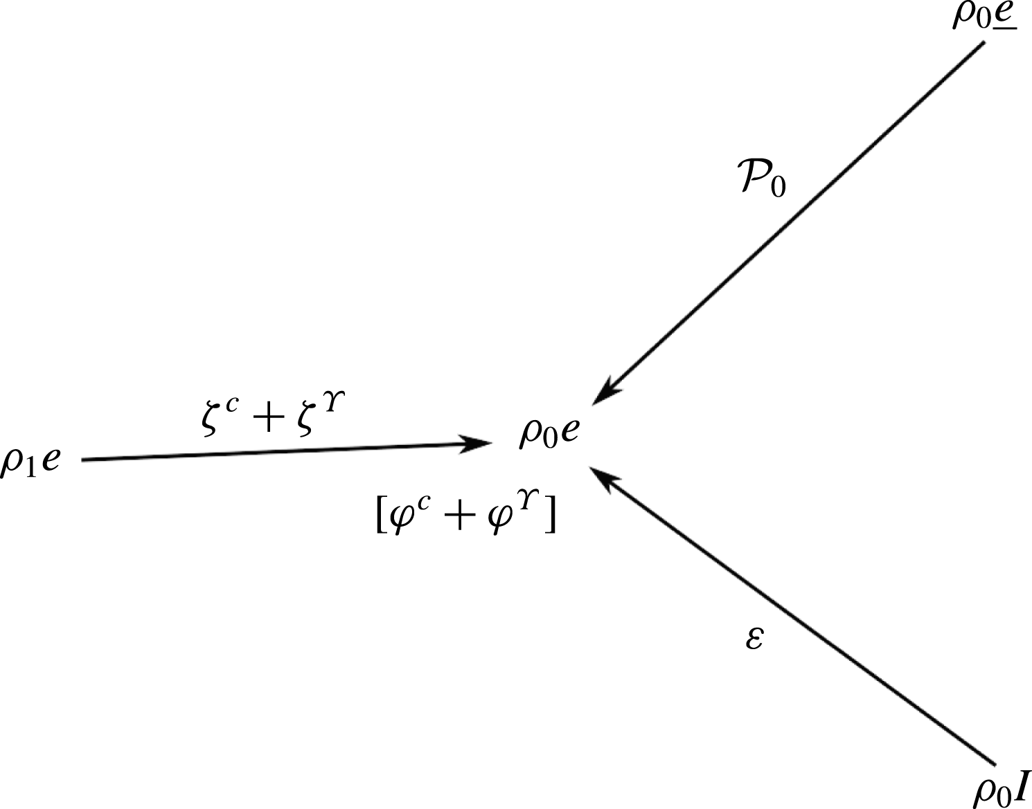
are represented in figure 2.
In this paper, the statistical average of these instantaneous energy exchanges are considered. This ensures the consistency of the formulation, in the sense that the energy exchanges in both the instantaneous and statistically averaged cases are well defined and are not conflicting. This consistency is important to give a physical interpretation to the energy exchange, as this lets us consider the statistically averaged energy exchanges as the statistical average of the associated instantaneous energy exchanges. The schematic representation of the energy exchanges in the statistically averaged case is not presented as it is identical, albeit with the addition of the statistical average.
Schematic representation of the energy exchanges associated with the ‘constant density turbulence kinetic energy’
 $\unicode[STIX]{x1D70C}_{0}e$
, identical to the half-trace of the velocity fluctuation correlation tensor
 $\unicode[STIX]{x1D65A}$
up to the constant scalar factor
 $\unicode[STIX]{x1D70C}_{0}$
.

The energy exchanges associated with the half-trace of the velocity fluctuation correlation tensor are decomposed in the particular case of a fully developed channel flow to recover the terms remaining in flows with constant fluid properties (here denoted with subscript
 $I$
). The terms specific to flows with variable fluid properties (here denoted with subscript
 $\unicode[STIX]{x1D6E4}$
) arise from the flow compressibility, the variations or fluctuations of the fluid properties and the presence of a mean wall-normal velocity. The mean wall-normal velocity
 $\overline{U}_{y}$
differs from zero in the compressible variable density channel with the classical averaging because it is in balance with the turbulent mass flux,
 $\overline{\unicode[STIX]{x1D70C}}\overline{U}_{y}=-\overline{\unicode[STIX]{x1D70C}^{\prime }u_{y}^{\prime }}$
. With a mass-weighted averaging, the mean wall-normal velocity is equal to zero. The study is then extended to the spectral domain. Since the flow is periodic in the streamwise and spanwise directions, any physical quantity
 $g(x,y,z)$
can be expressed as a Fourier series. We define and denote with the hat operator (
 $\widehat{\phantom{a}}$
) the Fourier coefficients of the Fourier series expansion of
 $g$
(see e.g. Lesieur Reference Lesieur2008):
 $$\begin{eqnarray}\widehat{g}(\boldsymbol{k},y,t)=\frac{1}{L_{x}L_{z}}\int _{0}^{L_{x}}\int _{0}^{L_{z}}g(\boldsymbol{x},y,t)\text{e}^{-\text{i}\boldsymbol{k}\boldsymbol{\cdot }\boldsymbol{x}}\,\text{d}\boldsymbol{x},\end{eqnarray}$$
where
 $\boldsymbol{x}=(x,z)$
is the position vector in the
 $xOz$
plane and
 $\boldsymbol{k}=(k_{x},k_{z})$
is the position vector in the
 $k_{x}Ok_{z}$
plane. In the spectral domain, we study the terms of the evolution equation of
 $$\begin{eqnarray}{\check{e}}={\textstyle \frac{1}{2}}\widehat{u_{i}^{\prime }}^{\ast }\widehat{u_{i}^{\prime }}.\end{eqnarray}$$
The spectral analysis extends each term of the spatial decomposition to the spectral domain, associating each of them with a corresponding term of the spectral decomposition. In addition, a purely spectral term is identified in the spectral decomposition, that is a spectral term with no spatial contribution.
To summarize the spatial and spectral decompositions, let us compare below the evolution equation of the half-trace of the velocity correlation tensor in the spatial and spectral domains. It is given in the spatial domain by
 $$\begin{eqnarray}\displaystyle {\displaystyle \frac{\unicode[STIX]{x2202}\overline{e}}{\unicode[STIX]{x2202}t}} & = & \displaystyle \overline{\unicode[STIX]{x1D711}}+\overline{{\mathcal{P}}}+\overline{\unicode[STIX]{x1D701}}+\overline{\unicode[STIX]{x1D700}}\nonumber\\ \displaystyle & = & \displaystyle \overline{\unicode[STIX]{x1D711}_{I}}+\overline{\unicode[STIX]{x1D711}_{\unicode[STIX]{x1D6E4}}}+\overline{{\mathcal{P}}_{I}}+\overline{{\mathcal{P}}_{\overline{U}_{y}}}+\overline{\unicode[STIX]{x1D701}}+\overline{\unicode[STIX]{x1D700}_{I}}+\overline{\unicode[STIX]{x1D700}_{\unicode[STIX]{x1D6E4}}}\end{eqnarray}$$
and in the spectral domain by
 $$\begin{eqnarray}\displaystyle {\displaystyle \frac{\unicode[STIX]{x2202}\overline{{\check{e}}}}{\unicode[STIX]{x2202}t}} & = & \displaystyle \overline{\check{\unicode[STIX]{x1D711}}}+\overline{\check{{\mathcal{P}}}}+\overline{\check{\unicode[STIX]{x1D701}}}+\overline{\check{\unicode[STIX]{x1D700}}}+\overline{\check{\unicode[STIX]{x1D6EF}}},\nonumber\\ \displaystyle & = & \displaystyle \overline{\check{\unicode[STIX]{x1D711}}_{I}}+\overline{\check{\unicode[STIX]{x1D711}}_{\unicode[STIX]{x1D6E4}}}+\overline{\check{{\mathcal{P}}}_{I}}+\overline{\check{{\mathcal{P}}}_{\overline{U}_{y}}}+\overline{\check{\unicode[STIX]{x1D701}}}+\overline{\check{\unicode[STIX]{x1D700}}_{I}}+\overline{\check{\unicode[STIX]{x1D700}}_{\unicode[STIX]{x1D6E4}}}+\overline{\check{\unicode[STIX]{x1D6EF}}},\end{eqnarray}$$
with
 $$\begin{eqnarray}\displaystyle \begin{array}{@{}rclrcl@{}}\overline{\unicode[STIX]{x1D711}_{I}}\ & =\ & \overline{\unicode[STIX]{x1D711}_{I}^{c}}+\overline{\unicode[STIX]{x1D711}_{I}^{p}}+\overline{\unicode[STIX]{x1D711}_{I,1}^{\unicode[STIX]{x1D708}}}+\overline{\unicode[STIX]{x1D711}_{I,2}^{\unicode[STIX]{x1D708}}}\qquad \qquad & \overline{\check{\unicode[STIX]{x1D711}}_{I}}\ & =\ & \overline{\check{\unicode[STIX]{x1D711}}_{I}^{c}}+\overline{\check{\unicode[STIX]{x1D711}}_{I}^{p}}+\overline{\check{\unicode[STIX]{x1D711}}_{I,1}^{\unicode[STIX]{x1D708}}}+\overline{\check{\unicode[STIX]{x1D711}}_{I,2}^{\unicode[STIX]{x1D708}}}\\ \overline{\unicode[STIX]{x1D700}_{I}}\ & =\ & \overline{\unicode[STIX]{x1D700}_{I,1}^{\unicode[STIX]{x1D708}}}+\overline{\unicode[STIX]{x1D700}_{I,2}^{\unicode[STIX]{x1D708}}}\qquad \qquad & \overline{\check{\unicode[STIX]{x1D700}}_{I}}\ & =\ & \overline{\check{\unicode[STIX]{x1D700}}_{I,1}}+\overline{\check{\unicode[STIX]{x1D700}}_{I,2}}\\ \overline{\unicode[STIX]{x1D711}_{\unicode[STIX]{x1D6E4}}}\ & =\ & \overline{\unicode[STIX]{x1D711}_{\overline{U}_{y}}^{c}}+\overline{\unicode[STIX]{x1D711}_{\unicode[STIX]{x2202}\overline{\unicode[STIX]{x1D70C}}}^{p}}+\overline{\unicode[STIX]{x1D711}_{\unicode[STIX]{x1D70C}^{\prime }}^{p}}+\overline{\unicode[STIX]{x1D711}_{\unicode[STIX]{x1D717}^{\prime },2}^{\unicode[STIX]{x1D708}}}\qquad \qquad & \overline{\check{\unicode[STIX]{x1D711}}_{\unicode[STIX]{x1D6E4}}}\ & =\ & \overline{\check{\unicode[STIX]{x1D711}}_{\overline{U}_{y}}^{c}}+\overline{\check{\unicode[STIX]{x1D711}}_{\unicode[STIX]{x2202}\overline{\unicode[STIX]{x1D70C}}}^{p}}+\overline{\check{\unicode[STIX]{x1D711}}_{\unicode[STIX]{x1D70C}^{\prime }}^{p}}+\overline{\check{\unicode[STIX]{x1D711}}_{\unicode[STIX]{x1D717}^{\prime },2}^{\unicode[STIX]{x1D708}}}\\ \ & \ & +\,\overline{\unicode[STIX]{x1D711}_{\unicode[STIX]{x2202}\overline{\unicode[STIX]{x1D708}},1}^{\unicode[STIX]{x1D708}}}+\overline{\unicode[STIX]{x1D711}_{\unicode[STIX]{x2202}\overline{\unicode[STIX]{x1D708}},2}^{\unicode[STIX]{x1D708}}}+\overline{\unicode[STIX]{x1D711}_{\unicode[STIX]{x1D708}^{\prime },1}^{\unicode[STIX]{x1D708}}}\qquad \qquad & \ & \ & +\,\overline{\check{\unicode[STIX]{x1D711}}_{\unicode[STIX]{x2202}\overline{\unicode[STIX]{x1D708}},1}^{\unicode[STIX]{x1D708}}}+\overline{\check{\unicode[STIX]{x1D711}}_{\unicode[STIX]{x2202}\overline{\unicode[STIX]{x1D708}},2}^{\unicode[STIX]{x1D708}}}+\overline{\check{\unicode[STIX]{x1D711}}_{\unicode[STIX]{x1D708}^{\prime },1}^{\unicode[STIX]{x1D708}}}\\ \ & \ & +\,\overline{\unicode[STIX]{x1D711}_{\unicode[STIX]{x1D708}^{\prime },2}^{\unicode[STIX]{x1D708}}}+\overline{\unicode[STIX]{x1D711}_{\unicode[STIX]{x1D6E9}}^{\unicode[STIX]{x1D708}}}\qquad \qquad & \ & \ & +\,\overline{\check{\unicode[STIX]{x1D711}}_{\unicode[STIX]{x1D708}^{\prime },2}^{\unicode[STIX]{x1D708}}}+\overline{\check{\unicode[STIX]{x1D711}}_{\unicode[STIX]{x1D6E9}}^{\unicode[STIX]{x1D708}}}\\ \overline{\unicode[STIX]{x1D701}}\ & =\ & \overline{\unicode[STIX]{x1D701}_{\overline{\unicode[STIX]{x1D6E9}}}^{c}}+\overline{\unicode[STIX]{x1D701}_{\unicode[STIX]{x1D717}^{\prime }}^{c}}+\overline{\unicode[STIX]{x1D701}_{\unicode[STIX]{x2202}\unicode[STIX]{x1D70C}}^{p}}+\overline{\unicode[STIX]{x1D701}_{\unicode[STIX]{x2202}\unicode[STIX]{x1D70C},1}^{\unicode[STIX]{x1D708}}}\qquad \qquad & \overline{\check{\unicode[STIX]{x1D701}}}\ & =\ & \overline{\check{\unicode[STIX]{x1D701}}_{\overline{\unicode[STIX]{x1D6E9}}}^{c}}+\overline{\check{\unicode[STIX]{x1D701}}_{\unicode[STIX]{x1D717}^{\prime }}^{c}}+\overline{\check{\unicode[STIX]{x1D701}}_{\unicode[STIX]{x2202}\unicode[STIX]{x1D70C}}^{p}}+\overline{\check{\unicode[STIX]{x1D701}}_{\unicode[STIX]{x2202}\unicode[STIX]{x1D70C},1}^{\unicode[STIX]{x1D708}}}\\ \ & \ & +\,\overline{\unicode[STIX]{x1D701}_{\unicode[STIX]{x2202}\unicode[STIX]{x1D70C},2}^{\unicode[STIX]{x1D708}}}+\overline{\unicode[STIX]{x1D701}_{\unicode[STIX]{x1D6E9}}^{\unicode[STIX]{x1D708}}}\qquad \qquad & \ & \ & +\,\overline{\check{\unicode[STIX]{x1D701}}_{\unicode[STIX]{x2202}\unicode[STIX]{x1D70C},2}^{\unicode[STIX]{x1D708}}}+\overline{\check{\unicode[STIX]{x1D701}}_{\unicode[STIX]{x1D6E9}}^{\unicode[STIX]{x1D708}}}\\ \overline{\unicode[STIX]{x1D700}_{\unicode[STIX]{x1D6E4}}}\ & =\ & \overline{\unicode[STIX]{x1D700}_{\unicode[STIX]{x1D717}^{\prime }}^{p}}+\overline{\unicode[STIX]{x1D700}_{\unicode[STIX]{x1D708}^{\prime },1}^{\unicode[STIX]{x1D708}}}+\overline{\unicode[STIX]{x1D700}_{\unicode[STIX]{x1D708}^{\prime },2}^{\unicode[STIX]{x1D708}}}+\overline{\unicode[STIX]{x1D700}_{\unicode[STIX]{x1D6E9}}^{\unicode[STIX]{x1D708}}}\qquad \qquad & \overline{\check{\unicode[STIX]{x1D700}}_{\unicode[STIX]{x1D6E4}}}\ & =\ & \overline{\check{\unicode[STIX]{x1D700}}_{\unicode[STIX]{x1D717}^{\prime }}^{p}}+\overline{\check{\unicode[STIX]{x1D700}}_{\unicode[STIX]{x1D708}^{\prime },1}}+\overline{\check{\unicode[STIX]{x1D700}}_{\unicode[STIX]{x1D708}^{\prime },2}}+\overline{\check{\unicode[STIX]{x1D700}}_{\unicode[STIX]{x1D6E9}}}\end{array} & & \displaystyle \nonumber\end{eqnarray}$$
and:


The terms are expressed using the symmetries of the flow and its homogeneity in the streamwise and spanwise directions to simplify the writing (
 $(\unicode[STIX]{x2202}\overline{\,\cdot \,}/\unicode[STIX]{x2202}x)=(\unicode[STIX]{x2202}\overline{\,\cdot \,}/\unicode[STIX]{x2202}z)=0$
and
 $\overline{U}_{z}=0$
). In particular, only the terms that do not have a zero theoretical value are considered. For instance, we only take into account the terms
 $(i=x,j=y)$
and
 $(i=y,j=y)$
of the production
 $\overline{{\mathcal{P}}}=-\overline{u_{i}^{\prime }u_{j}^{\prime }}(\unicode[STIX]{x2202}\overline{U}_{i}/\unicode[STIX]{x2202}x_{j})$
, since the other terms are theoretically equal to zero.
In the incompressible case, only the incompressible terms remain. The evolution equation of the half-trace of the velocity correlation tensor reduces in the spatial domain to
 $$\begin{eqnarray}{\displaystyle \frac{\unicode[STIX]{x2202}\overline{e}}{\unicode[STIX]{x2202}t}}=\overline{\unicode[STIX]{x1D711}_{I}^{c}}+\overline{\unicode[STIX]{x1D711}_{I}^{p}}+\overline{\unicode[STIX]{x1D711}_{I,1}^{\unicode[STIX]{x1D708}}}+\overline{\unicode[STIX]{x1D711}_{I,2}^{\unicode[STIX]{x1D708}}}+\overline{{\mathcal{P}}_{I}}+\overline{\unicode[STIX]{x1D700}_{I,1}^{\unicode[STIX]{x1D708}}}+\overline{\unicode[STIX]{x1D700}_{I,2}^{\unicode[STIX]{x1D708}}}\end{eqnarray}$$
and in the spectral domain to
 $$\begin{eqnarray}{\displaystyle \frac{\unicode[STIX]{x2202}\overline{{\check{e}}}}{\unicode[STIX]{x2202}t}}=\overline{\check{\unicode[STIX]{x1D711}}_{I}^{c}}+\overline{\check{\unicode[STIX]{x1D711}}_{I}^{p}}+\overline{\check{\unicode[STIX]{x1D711}}_{I,1}^{\unicode[STIX]{x1D708}}}+\overline{\check{\unicode[STIX]{x1D711}}_{I,2}^{\unicode[STIX]{x1D708}}}+\overline{\check{{\mathcal{P}}}_{I}}+\overline{\check{\unicode[STIX]{x1D700}}_{I,1}}+\overline{\check{\unicode[STIX]{x1D700}}_{I,2}}+\overline{\check{\unicode[STIX]{x1D6EF}}}.\end{eqnarray}$$
In flows with highly variable fluid properties, additional terms appear. Nevertheless, they originate from distinct flow characteristics. The thermal terms may appear because of the addition of a wall-normal mean velocity
 $\overline{U}_{y}$
, come from the flow dilatation
 $\unicode[STIX]{x1D6E9}$
, or lie in variations or fluctuations of the fluid properties, namely the viscosity and the density.
3 Study configuration
To provide the data necessary to compute the terms of the evolution equation of the half-trace of the velocity fluctuation correlation tensor, a direct numerical simulation of a fully developed channel flow is carried out. In the following, we describe the flow, the geometry, the numerical settings and the numerical tools used. Then, we validate the numerical method in the incompressible case.
3.1 Channel flow configuration
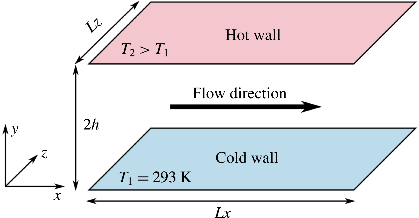
We consider a fully developed turbulent air flow under a strong temperature gradient in a rectangular channel, as represented in figure 3. The channel is periodic in both the streamwise (
 $x$
) and spanwise (
 $z$
) directions. The channel walls are at constant temperature. The temperature of the hot wall is
 $T_{2}=586$
K and the temperature of the cold wall is
 $T_{1}=293$
K. This creates a temperature gradient in the wall-normal direction (
 $y$
). The flow is fully developed despite non-adiabatic wall conditions because the heat flux at the hot and cold wall exactly balance out. The mean friction Reynolds number is
 $Re_{\unicode[STIX]{x1D70F}}=180$
. Let us define this quantity. The friction Reynolds number at each wall is defined as
 $$\begin{eqnarray}Re_{\unicode[STIX]{x1D70F}}=\frac{U_{\unicode[STIX]{x1D70F}}h}{\unicode[STIX]{x1D708}_{\unicode[STIX]{x1D714}}},\end{eqnarray}$$
with
 $h$
the half-height of the channel,
 $\unicode[STIX]{x1D708}_{\unicode[STIX]{x1D714}}$
the cinematic viscosity at the wall and
 $U_{\unicode[STIX]{x1D70F}}$
the friction velocity
 $$\begin{eqnarray}U_{\unicode[STIX]{x1D70F}}=\sqrt{\unicode[STIX]{x1D708}_{\unicode[STIX]{x1D714}}\left({\displaystyle \frac{\unicode[STIX]{x2202}\overline{U}_{x}}{\unicode[STIX]{x2202}y}}\right)_{\unicode[STIX]{x1D714}}}.\end{eqnarray}$$
The friction Reynolds numbers at the hot and cold wall are different, since the value of the friction velocity and the properties of the fluid differ. The mean friction Reynolds number is defined as the average of the friction Reynolds number computed at the cold and hot side.
The same channel is also studied in the isothermal case. In this case, both wall are at the cold temperature. The same friction Reynolds number is considered. This results in a 20 % lower mass flow rate. Hereafter, we will refer to the channel flow configuration in which the channel is subjected to a strong temperature gradient as the anisothermal configuration and the configuration in which both wall are at the same temperature as the isothermal configuration.
Biperiodic anisothermal channel flow.

3.2 Governing equations
The above-described flow is weakly turbulent. The mean Mach number is 0.008. Compressibility effects due to velocity are therefore negligible. Large variations of the fluid properties are generated by the temperature gradient. These considerations let us use Paolucci’s method (Paolucci Reference Paolucci1982) to remove acoustic effects from the Navier–Stokes equations. Each variable of the Navier–Stokes equations is written as a power series of the squared Mach number. Then, the smaller-order terms of each equation are kept. The resulting low Mach number equations split the pressure in two parts: the thermodynamical pressure
 $P_{0}$
and the mechanical pressure
 $P$
. The constant in space thermodynamical pressure
 $P_{0}$
is the mean pressure in the domain. The mechanical pressure is the pressure induced by momentum variations. The effects of gravity are neglected and air is considered as an ideal gas for the purpose of this study.
Since the channel flow is periodic in the streamwise direction, no pressure gradient appears through the boundary conditions to balance out the dissipative forces. A streamwise volume force
 $f$
is added to the momentum conservation equation in order to replicate the effect of a pressure gradient.
Given the above considerations, we use the following set of equations:
-
(i) mass conservation equation
(3.3)
$$\begin{eqnarray}{\displaystyle \frac{\unicode[STIX]{x2202}\unicode[STIX]{x1D70C}}{\unicode[STIX]{x2202}t}}+{\displaystyle \frac{\unicode[STIX]{x2202}\unicode[STIX]{x1D70C}U_{j}}{\unicode[STIX]{x2202}x_{j}}}=0;\end{eqnarray}$$
-
(ii) momentum conservation equation
(3.4)
$$\begin{eqnarray}{\displaystyle \frac{\unicode[STIX]{x2202}\unicode[STIX]{x1D70C}U_{i}}{\unicode[STIX]{x2202}t}}+{\displaystyle \frac{\unicode[STIX]{x2202}\unicode[STIX]{x1D70C}U_{j}U_{i}}{\unicode[STIX]{x2202}x_{j}}}=-{\displaystyle \frac{\unicode[STIX]{x2202}P}{\unicode[STIX]{x2202}x_{i}}}+{\displaystyle \frac{\unicode[STIX]{x2202}}{\unicode[STIX]{x2202}x_{j}}}\left[\unicode[STIX]{x1D707}\left({\displaystyle \frac{\unicode[STIX]{x2202}U_{i}}{\unicode[STIX]{x2202}x_{j}}}+{\displaystyle \frac{\unicode[STIX]{x2202}U_{j}}{\unicode[STIX]{x2202}x_{i}}}\right)\right]-\frac{2}{3}{\displaystyle \frac{\unicode[STIX]{x2202}}{\unicode[STIX]{x2202}x_{i}}}\left(\unicode[STIX]{x1D707}{\displaystyle \frac{\unicode[STIX]{x2202}U_{j}}{\unicode[STIX]{x2202}x_{j}}}\right)+f\unicode[STIX]{x1D6FF}_{ix};\end{eqnarray}$$
-
(iii) energy conservation equation
(3.5)
$$\begin{eqnarray}\unicode[STIX]{x1D70C}C_{p}\left({\displaystyle \frac{\unicode[STIX]{x2202}T}{\unicode[STIX]{x2202}t}}+U_{j}{\displaystyle \frac{\unicode[STIX]{x2202}T}{\unicode[STIX]{x2202}x_{j}}}\right)={\displaystyle \frac{\unicode[STIX]{x2202}P_{0}}{\unicode[STIX]{x2202}t}}+{\displaystyle \frac{\unicode[STIX]{x2202}}{\unicode[STIX]{x2202}x_{j}}}\left(\unicode[STIX]{x1D706}{\displaystyle \frac{\unicode[STIX]{x2202}T}{\unicode[STIX]{x2202}x_{j}}}\right);\end{eqnarray}$$
-
(iv) ideal gas law
(3.6)
$$\begin{eqnarray}P_{0}=\unicode[STIX]{x1D70C}rT;\end{eqnarray}$$
-
(v) thermodynamic pressure homogeneity
(3.7)
$$\begin{eqnarray}{\displaystyle \frac{\unicode[STIX]{x2202}P_{0}}{\unicode[STIX]{x2202}x_{i}}}=0,\end{eqnarray}$$


with
 $\unicode[STIX]{x1D70C}$
the density,
 $T$
the temperature,
 $\unicode[STIX]{x1D707}$
the dynamic viscosity,
 $\unicode[STIX]{x1D706}$
the thermal conductivity,
 $C_{p}$
the heat capacity at constant pressure,
 $r$
the ideal gas specific constant,
 $t$
the time,
 $P$
the mechanical pressure,
 $P_{0}$
the thermodynamical pressure,
 $U_{i}$
the
 $i$
th component of velocity and
 $x_{i}$
the Cartesian coordinate in the
 $i$
-direction. Einstein summation convention is used and
 $\unicode[STIX]{x1D6FF}_{ij}$
is the Kronecker delta.
We use Sutherland’s law (Sutherland Reference Sutherland1893) to compute the fluid properties
 $$\begin{eqnarray}\displaystyle & \displaystyle \unicode[STIX]{x1D707}(T)=\unicode[STIX]{x1D707}_{0}\left(\frac{T}{T_{0}}\right)^{3/2}\frac{T_{0}+S}{T+S}, & \displaystyle\end{eqnarray}$$
 $$\begin{eqnarray}\displaystyle & \displaystyle \unicode[STIX]{x1D706}(T)=\frac{C_{p}}{Pr}\unicode[STIX]{x1D707}(T), & \displaystyle\end{eqnarray}$$
with
 $\unicode[STIX]{x1D707}_{0}=1.716\times 10^{-5}$
,
 $S=110.4$
and
 $T_{0}=273.15$
K. The Prandtl number and the heat capacity at constant pressure are assumed constant, with
 $Pr=0.76$
and
 $C_{p}=1005~\text{J}~\text{kg}^{-1}~\text{K}^{-1}$
. The ideal gas specific constant is
 $r=287~\text{J}~\text{kg}^{-1}~\text{K}^{-1}$
.
3.3 Numerical setting
The mesh is regular in both homogeneous directions and follows a hyperbolic tangent law in the wall-normal direction. The wall-normal grid coordinates are symmetrical with respect to the plane
 $y=h$
. In the first half of the channel, they are given by
 $$\begin{eqnarray}y_{k}=h\left(1+\frac{1}{a}\tanh \left[\left(\frac{k-1}{N_{y}-1}-1\right)\tanh ^{-1}(a)\right]\right),\end{eqnarray}$$
where
 $a$
is the mesh dilatation constant and
 $N_{y}$
the number of grid points in the wall-normal direction.
The same mesh is used in the anisothermal and isothermal simulations. It contains
 $384\times 266\times 384$
cells. The resulting cell sizes in wall units are
 $\unicode[STIX]{x1D6E5}_{x}^{+}=5.8$
,
 $\unicode[STIX]{x1D6E5}_{y}^{+}=0.085$
at the wall and 2.9 at the centre and
 $\unicode[STIX]{x1D6E5}_{z}^{+}=2.9$
in the isothermal case;
 $\unicode[STIX]{x1D6E5}_{x}^{+}=8.5$
,
 $\unicode[STIX]{x1D6E5}_{y}^{+}=0.13$
at the wall and 4.2 at the centre and
 $\unicode[STIX]{x1D6E5}_{z}^{+}=4.2$
in the anisothermal case. Given the mesh precision, a no-slip boundary condition is used at the walls. The domain size is:
 $L_{x}=4\unicode[STIX]{x03C0}h$
,
 $L_{y}=2h$
and
 $L_{z}=2\unicode[STIX]{x03C0}h$
with
 $h=15$
mm.
To solve the set of (3.3)–(3.7), we use a finite difference method written in a divergence form in a staggered grid system (Morinishi et al. Reference Morinishi, Lundhomas, Vasilyev and Moin1998; Nicoud Reference Nicoud2000). The time scheme is a third-order Runge–Kutta (Williamson Reference Williamson1980). A fourth-order centred scheme is used for momentum convection and a third-order upstream scheme is used for temperature convection (Leonard Reference Leonard1979). This is performed using the TrioCFD software (Calvin, Cueto & Emonot Reference Calvin, Cueto and Emonot2002). This software was used in many direct numerical simulations of fluid flow coupled with other physical phenomena (Brillant et al. Reference Brillant, Husson, Bataille and Ducros2008; Toutant et al. Reference Toutant, Labourasse, Lebaigue and Simonin2008; Chandesris et al. Reference Chandesris, d’Hueppe, Mathieu, Jamet and Goyeau2013; Toutant & Bataille Reference Toutant and Bataille2013).
The value of the volume force
 $f$
is adjusted through a control loop to keep the mass flow rate constant,
 $$\begin{eqnarray}f_{t+1}=f_{t}+C_{0}\frac{D_{target}-2D_{t}+D_{t-1}}{\unicode[STIX]{x0394}t},\end{eqnarray}$$
with
 $C_{0}$
a damping constant,
 $D$
the mass flow rate,
 $D_{target}$
the targeted mass flow rate and
 $t-1$
,
 $t$
and
 $t+1$
indices related to the previous, current and next time step respectively. A term associated with the forcing term
 $\overline{u_{x}^{\prime }\,f/\unicode[STIX]{x1D70C}}$
appears in the transport equation of the half-trace of the velocity correlation tensor. This term has been computed from the result of the direct numerical simulation and was found to be insignificant.
3.4 Data acquisition
The data acquisition is carried out in two steps because the computation of different terms of the evolution equation of the half-trace of the velocity fluctuation correlation tensor requires knowledge of mean and fluctuating quantities. First, statistics on the mean velocities, temperature and pressure are acquired. Full convergence is attained after a total duration of
 $3.59$
s in the isothermal case (29 characteristic time
 $h/U_{\unicode[STIX]{x1D70F}}$
) and
 $2.86$
s in the anisothermal case (34 characteristic time, using the cold wall friction velocity). Once this prior step completed, the data collection is carried out and spans over a total duration of
 $7.95$
s in the isothermal case (64 characteristic time) and
 $3.16$
s in the anisothermal case (37 characteristic time).
To compute the spectral terms, we use the discrete two-dimensional Fourier transform
 $$\begin{eqnarray}\widehat{g}(k_{x,m},y,k_{z,n})=\frac{1}{N_{x}N_{z}}\mathop{\sum }_{p=0}^{N_{x}-1}\mathop{\sum }_{k=0}^{N_{z}-1}g(x_{p},y,z_{k})\exp \left(-2\unicode[STIX]{x03C0}\text{i}\left(\frac{mp}{N_{x}}+\frac{kn}{N_{z}}\right)\right).\end{eqnarray}$$
The Fourier transform is carried out in the streamwise and spanwise directions only. The time averaged spectral terms depends on the three parameters
 $k_{x}$
,
 $y$
and
 $k_{z}$
. In order to simplify the interpretation of the terms, only the dependence on the wavenumber norm at each wall-normal coordinate will be considered. This removes from the scope of this study the spectral directionality of the energy transfers.
3.5 Wavenumber bin
The two-dimensional spectral results are analysed using wavenumber bins following Bolotnov et al. (Reference Bolotnov, Lahey, Drew, Jansen and Oberai2010). The procedure used is as follows: the wavenumber space is divided in
 $N_{b}$
annulus-shaped wavenumber bins. The bin #
 $i$
contains every wavenumber vector
 $\boldsymbol{k}$
whose norm
 $k$
ranges between
 $k_{i}$
and
 $k_{i+1}$
, the lower and upper bound of the bin #
 $i$
. For each term, we then assign to the bin #
 $i$
(at its wavenumber centre
 $k_{c,i}$
) the sum of the values of the term computed at each wavenumber contained in the bin.
Wavenumber bins kill any directionality of the energy transfers since only the wavenumber norm is taken into account. This is only correctly done if the bin contains a large number of wavenumber vectors and the distribution of the wavenumber vectors is isotropic. Since the distribution of wavenumber bins is logarithmic and the distribution of wavenumber vectors is not, the number of wavenumber vectors per bin grows exponentially with the wavenumber bin number. This results in a low number of wavenumber vector per bin at low wavenumbers. To address this issue, a low pass filter was applied to the spectral data. This improves the quality of the statistics at low wavenumbers.
The use of wavenumber bins should be taken into account in the interpretation of the results. The values obtained are uniformly distributed on a logarithmic scale and integration over the wavenumber space is done by simple summation of the values. The use of wavenumber bins also reduces the dependence of the results on the domain size and mesh. On the other hand, the results are entirely determined by the bins construction.
Thereupon, in order to compare our results with Bolotnov et al. (Reference Bolotnov, Lahey, Drew, Jansen and Oberai2010), we use the same wavenumber bins. We define
 $N_{b}=24$
wavenumber bins of uniform length in logarithmic scale, with
 $$\begin{eqnarray}k_{i}=k_{min}\left(\frac{k_{max}}{k_{min}}\right)^{i/N_{b}},\end{eqnarray}$$
where
 $k_{min}=1~\text{m}^{-1}$
and
 $k_{max}=73~\text{m}^{-1}$
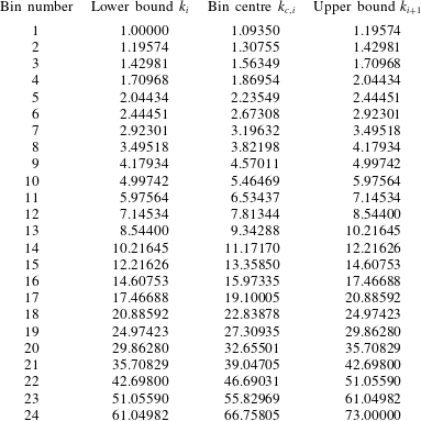
are the minimum and maximum bound across all bins. The bounds and centre of the wavenumber bins are given in table 1. Note that since the wavenumber bins are constructed with respect to the domain and mesh sizes of the direct numerical simulation of Trofimova et al. (Reference Trofimova, Tejada-Martínez, Jansen and Lahey2009) used by Bolotnov et al. (Reference Bolotnov, Lahey, Drew, Jansen and Oberai2010), they do not span over our entire computable wavenumber space. This excludes very small and very large wavenumbers. Nonetheless, we verified that no energy exchanges were located outside of the range of wavenumber bins.
Construction of the wavenumber bins.

3.6 Validation
The numerical set-up is validated in the isothermal configuration through a mesh convergence study. The simulation is carried out with three meshes later referred to as coarse mesh, medium mesh and fine mesh. The coarse mesh has
 $192\times 118\times 96$
cells. The cell sizes in wall units are
 $\unicode[STIX]{x1D6E5}_{x}^{+}=11.5$
,
 $\unicode[STIX]{x1D6E5}_{y}^{+}=0.17$
at the wall and 6.7 at the centre and
 $\unicode[STIX]{x1D6E5}_{z}^{+}=11.5$
. The medium mesh has
 $384\times 190\times 288$
cells. The cell sizes in wall units are
 $\unicode[STIX]{x1D6E5}_{x}^{+}=5.8$
,
 $\unicode[STIX]{x1D6E5}_{y}^{+}=0.16$
at the wall and 3.7 at the centre and
 $\unicode[STIX]{x1D6E5}_{z}^{+}=3.9$
. The fine mesh is described in § 3.3. The results are compared to the three following references from the literature: Moser et al. (Reference Moser, Kim and Mansour1999) and Vreman & Kuerten (Reference Vreman and Kuerten2014) in the spatial domain and Bolotnov et al. (Reference Bolotnov, Lahey, Drew, Jansen and Oberai2010) in the spectral domain. The three references are at the same friction Reynolds number of 180. The consistency of the spectral results is ensured by making sure that the integrated spectral data reduces to the correct spatial value.
3.6.1 Validation of the spatial turbulence kinetic energy terms
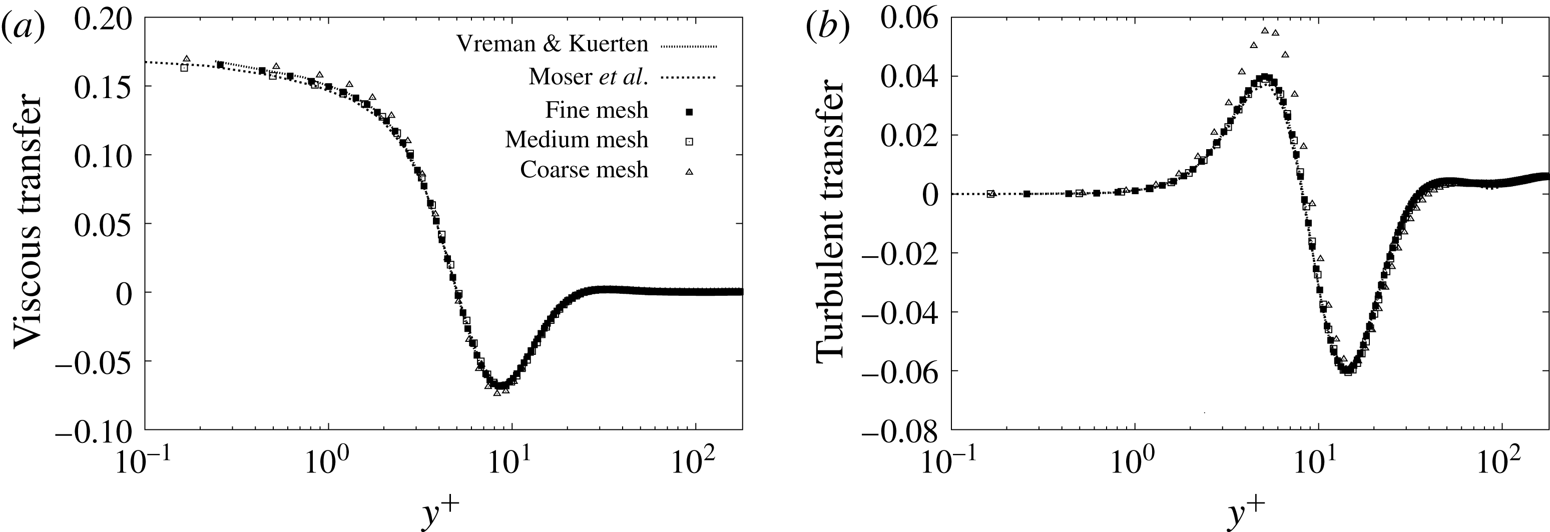
The turbulence kinetic energy is given in the incompressible case by the half-trace of the velocity fluctuation correlation tensor. The viscous transfer and the turbulent transfer, two terms of its evolution equation, are compared in the isothermal case to the results of Moser et al. (Reference Moser, Kim and Mansour1999) and Vreman & Kuerten (Reference Vreman and Kuerten2014) in figure 4. The values are scaled by
 ${U_{\unicode[STIX]{x1D70F}}}^{4}/\unicode[STIX]{x1D708}_{\unicode[STIX]{x1D714}}$
, where
 $U_{\unicode[STIX]{x1D70F}}$
is the friction velocity and
 $\unicode[STIX]{x1D708}_{\unicode[STIX]{x1D714}}$
the cinematic viscosity at the wall. The results show two things. First, the profiles associated with the medium and fine meshes are very close, indicating that the mesh convergence is attained. Second, the fine mesh profiles are nearly identical to the reference profiles of Vreman & Kuerten (Reference Vreman and Kuerten2014). The profiles of Moser et al. (Reference Moser, Kim and Mansour1999) deviate slightly from the profiles of Vreman & Kuerten (Reference Vreman and Kuerten2014) for the viscous transfer near to the wall. The results of Vreman & Kuerten (Reference Vreman and Kuerten2014) are believed to be the most accurate as they use a finer mesh and a longer averaging time. Hence, the data of Vreman & Kuerten (Reference Vreman and Kuerten2014) will from now on be used exclusively for the validation of the spatial terms.
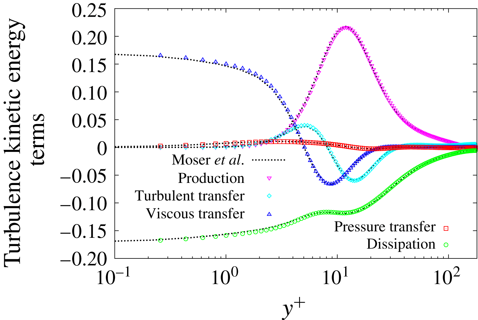
The mesh convergence study shows similar results for the other terms (not shown here). The comparison of the fine mesh profiles with the results of Vreman & Kuerten (Reference Vreman and Kuerten2014) is shown for each term in figure 5. The profile of each term is equal to the reference profile. This validates the spatial profiles of the terms of the evolution equation of the half-trace of the velocity fluctuation correlation tensor at the incompressible limit.
Validation of the profile of the viscous transfer
 $\overline{\unicode[STIX]{x1D708}}(\unicode[STIX]{x2202}^{2}\overline{e}/\unicode[STIX]{x2202}y^{2})$
(a) and of the turbulent transfer
 $-(\unicode[STIX]{x2202}\overline{eu_{y}^{\prime }}/\unicode[STIX]{x2202}y)$
(b).

Validation of the spatial turbulence kinetic energy terms. The terms are: the production
 $-\overline{u_{x}^{\prime }u_{y}^{\prime }}(\unicode[STIX]{x2202}\overline{U}_{x}/\unicode[STIX]{x2202}y)$
, the turbulent transfer
 $-(\unicode[STIX]{x2202}\overline{eu_{y}^{\prime }}/\unicode[STIX]{x2202}y)$
, the viscous transfer
 $\overline{\unicode[STIX]{x1D708}}(\unicode[STIX]{x2202}^{2}\overline{e}/\unicode[STIX]{x2202}y^{2})$
, the pressure transfer
 $-(1/\overline{\unicode[STIX]{x1D70C}})(\unicode[STIX]{x2202}/\unicode[STIX]{x2202}y)\overline{Pu_{y}^{\prime }}$
and the dissipation
 $-\overline{\unicode[STIX]{x1D708}}\overline{(\unicode[STIX]{x2202}u_{i}^{\prime }/\unicode[STIX]{x2202}x_{j})(\unicode[STIX]{x2202}u_{i}^{\prime }/\unicode[STIX]{x2202}x_{j})}$
.

3.6.2 Validation of the spectral turbulence kinetic energy terms
The numerical properties of the discrete Fourier transform used ensure that the summation of over all wavenumber bins of a spectral term for a given wall-normal coordinate
 $y$
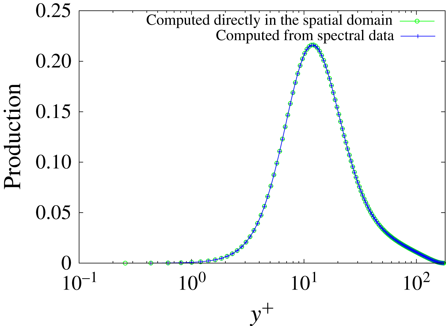
is equal to the value of the associated spatial term. This property is used to verify the consistency of the spectral and spatial data. The profiles of production computed from the spectral data and computed directly in the spatial domain are compared in figure 6 and are shown to be identical. This was verified to be true for all terms in the isothermal case and in the anisothermal case.
Production profile computed directly in the spatial domain,
 $-\overline{u_{x}^{\prime }u_{y}^{\prime }}(\unicode[STIX]{x2202}\overline{U}_{x}/\unicode[STIX]{x2202}y)$
, and computed from the spectral data,
 $\text{Re}(-\overline{\widehat{u_{x}^{\prime }}^{\ast }\widehat{u_{y}^{\prime }}}(\unicode[STIX]{x2202}\overline{U}_{x}/\unicode[STIX]{x2202}y))$
.

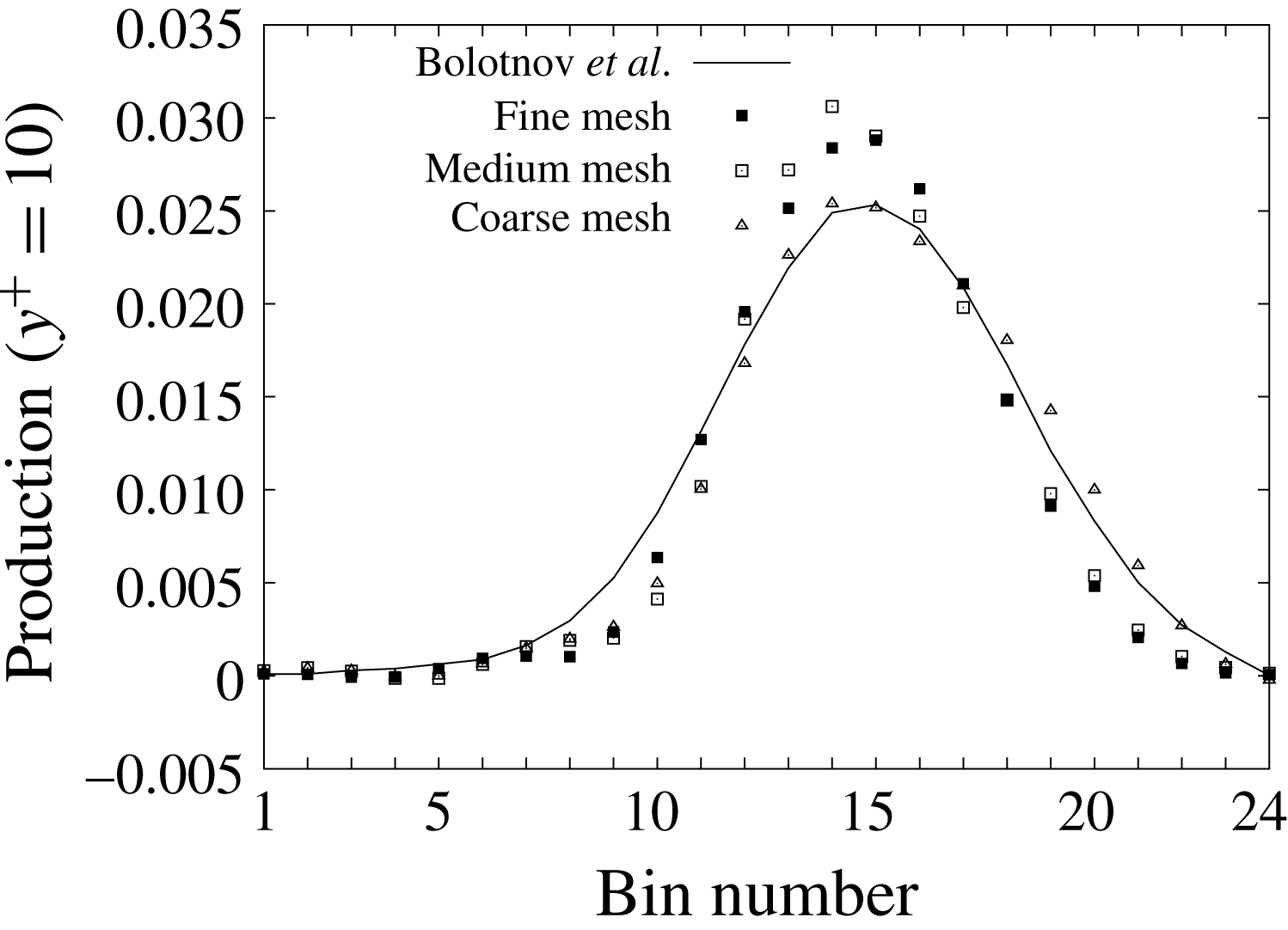
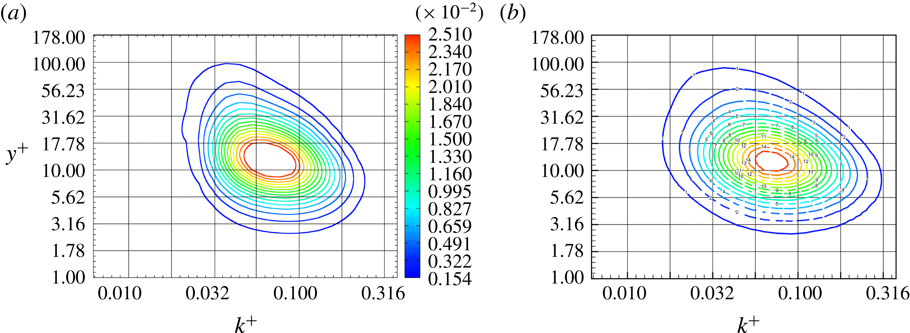
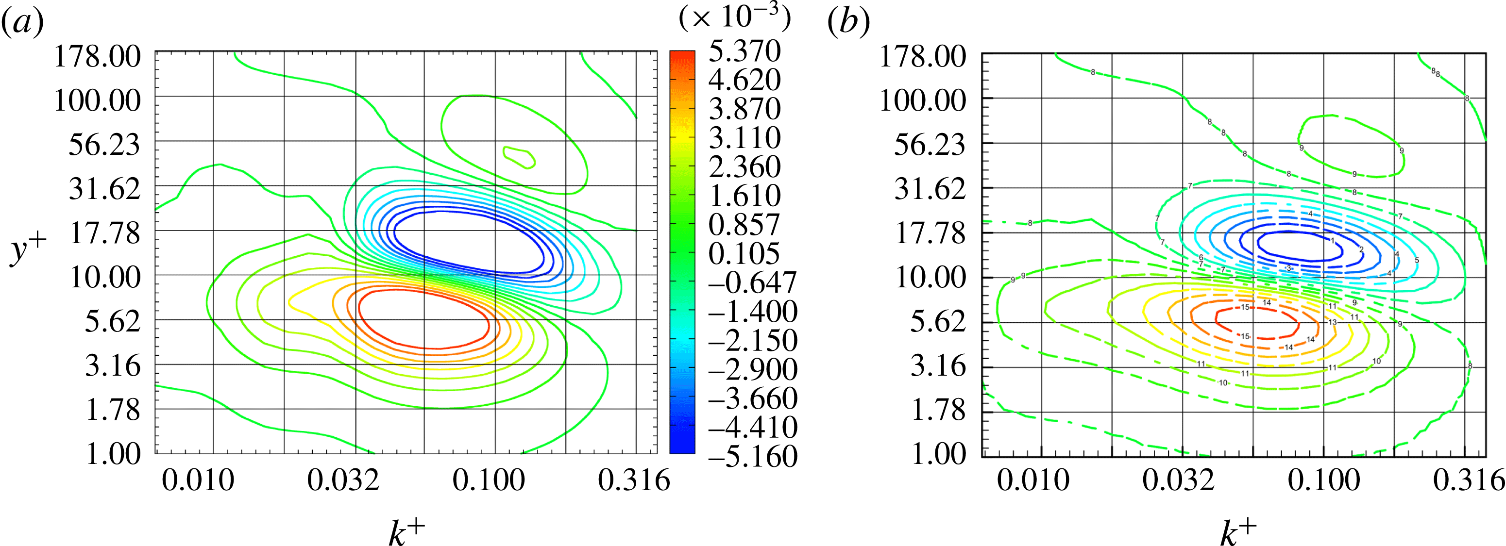
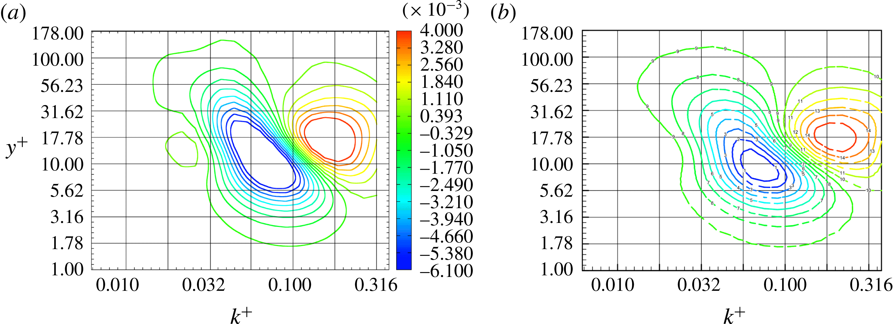
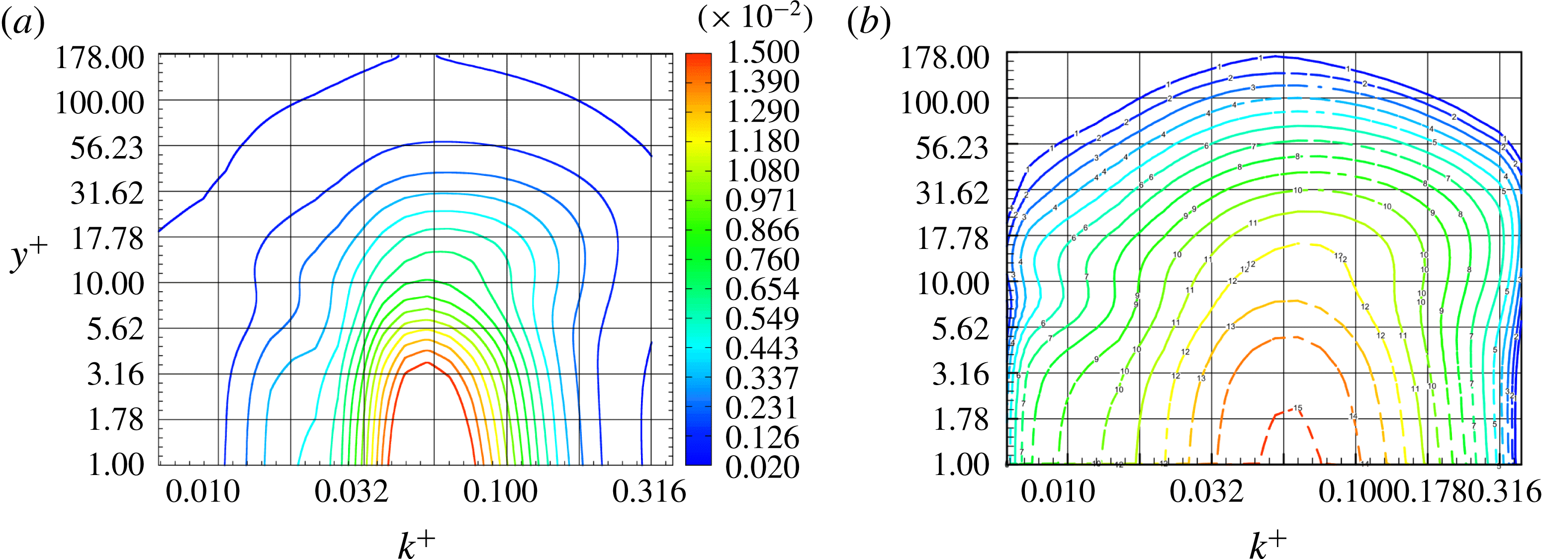
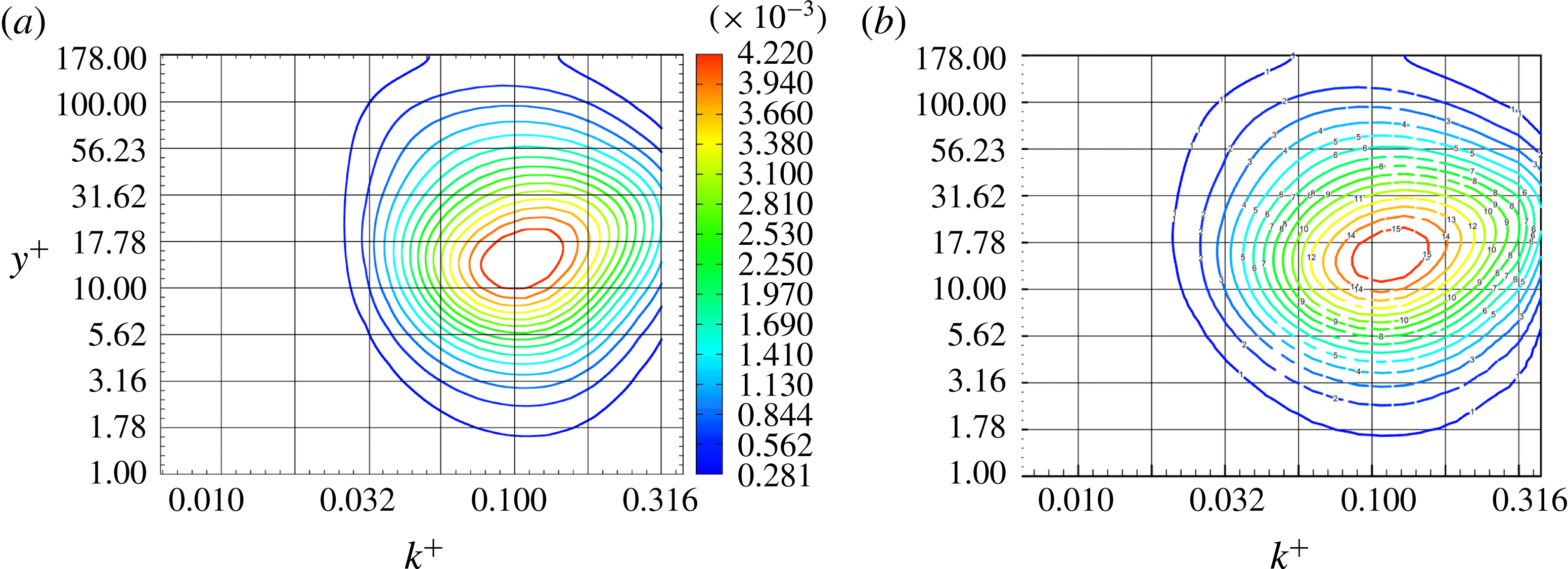
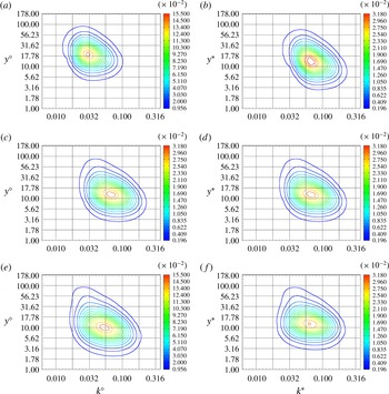
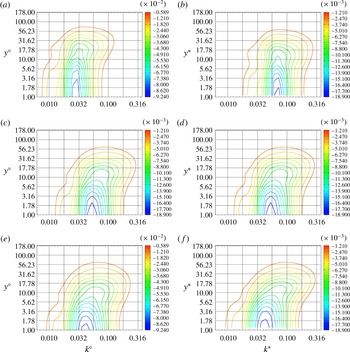
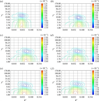
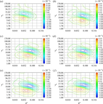
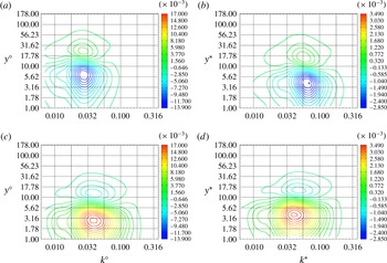
The spectral data are compared in the isothermal case to the results provided by Bolotnov et al. (Reference Bolotnov, Lahey, Drew, Jansen and Oberai2010). The figure 7 compares the spectral profiles of the production computed from the coarse, medium and fine meshes with Bolotnov et al. (Reference Bolotnov, Lahey, Drew, Jansen and Oberai2010) at a distance of 10 in wall units from the wall. The fine and medium profiles are very close showing a good convergence of the production statistical profile in the spectral domain. The results are in agreement with those of Bolotnov et al. (Reference Bolotnov, Lahey, Drew, Jansen and Oberai2010). The spectral profiles have the same shape and predict the same spectral location of the maximum value. There are however some differences. The profile of Bolotnov et al. (Reference Bolotnov, Lahey, Drew, Jansen and Oberai2010) has a lower amplitude and is more spread out in wavenumber. This leads to a very similar total integrated value, though not exactly identical. Unfortunately, there are no further data on the spectral turbulence kinetic energy terms in the literature to decide between the two profiles. Therefore, we compare the spatial integrated value of the two spectra. There is 3.5 %–4 % difference between the spatial integrated value of Bolotnov et al. (Reference Bolotnov, Lahey, Drew, Jansen and Oberai2010) and the results of Moser et al. (Reference Moser, Kim and Mansour1999) or Vreman & Kuerten (Reference Vreman and Kuerten2014), whereas the difference is less than 1 % for our spectrum. Our results are thus more accurate with regard to their total integrated value.
Validation of the spectral profile at
 $y^{+}=10$
of the production,
 $\text{Re}(-\overline{\widehat{u_{x}^{\prime }}^{\ast }\widehat{u_{y}^{\prime }}}(\unicode[STIX]{x2202}\overline{U}_{x}/\unicode[STIX]{x2202}y))$
.

Production,
 $\text{Re}(-\overline{\widehat{u_{x}^{\prime }}^{\ast }\widehat{u_{y}^{\prime }}}(\unicode[STIX]{x2202}\overline{U}_{x}/\unicode[STIX]{x2202}y))$
: (a) this paper; (b) Bolotnov et al.

Interplane triadic,
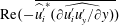 $\text{Re}(-\overline{\widehat{u_{i}^{\prime }}^{\ast }\widehat{(\unicode[STIX]{x2202}u_{i}^{\prime }u_{y}^{\prime }/\unicode[STIX]{x2202}y)}})$
: (a) this paper; (b) Bolotnov et al.

Inplane triadic,
 $\text{Re}(-\overline{\widehat{u_{i}^{\prime }}^{\ast }\widehat{(\unicode[STIX]{x2202}u_{i}^{\prime }u_{x}^{\prime }/\unicode[STIX]{x2202}x)}-\overline{\widehat{u_{i}^{\prime }}^{\ast }\widehat{(\unicode[STIX]{x2202}u_{i}^{\prime }u_{z}^{\prime }/\unicode[STIX]{x2202}z)}}})$
: (a) this paper; (b) Bolotnov et al.

Interplane dissipation,
 $\text{Re}(-\overline{\unicode[STIX]{x1D708}}\overline{\widehat{(\unicode[STIX]{x2202}u_{i}^{\prime }/\unicode[STIX]{x2202}y)}^{\ast }\widehat{(\unicode[STIX]{x2202}u_{i}^{\prime }/\unicode[STIX]{x2202}y)}})$
: (a) this paper; (b) Bolotnov et al.

Inplane dissipation,
 $\text{Re}(-\overline{\unicode[STIX]{x1D708}}\overline{\widehat{(\unicode[STIX]{x2202}u_{i}^{\prime }/\unicode[STIX]{x2202}x)}^{\ast }\widehat{(\unicode[STIX]{x2202}u_{i}^{\prime }/\unicode[STIX]{x2202}x)}}-\overline{\unicode[STIX]{x1D708}}\overline{\widehat{(\unicode[STIX]{x2202}u_{i}^{\prime }/\unicode[STIX]{x2202}z)}^{\ast }\widehat{(\unicode[STIX]{x2202}u_{i}^{\prime }/\unicode[STIX]{x2202}z)}})$
: (a) this paper; (b) Bolotnov et al.

Viscous transfer,
 $\text{Re}(\overline{\unicode[STIX]{x1D708}}(\unicode[STIX]{x2202}^{2}\overline{{\check{e}}}/\unicode[STIX]{x2202}y^{2}))$
: (a) this paper; (b) Bolotnov et al.

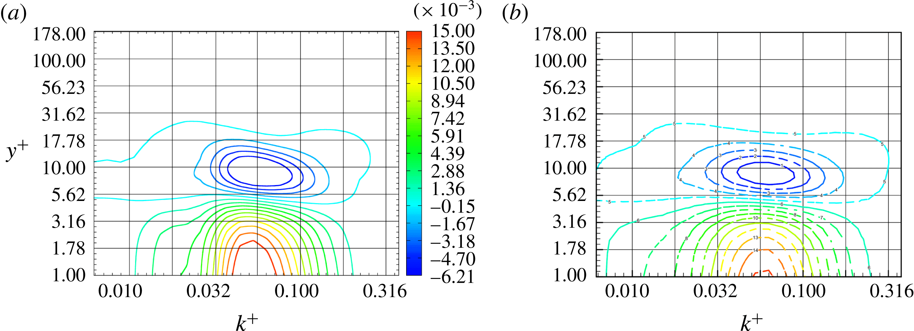
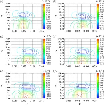
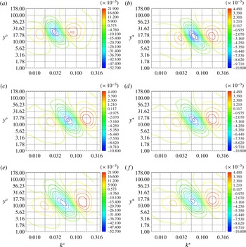
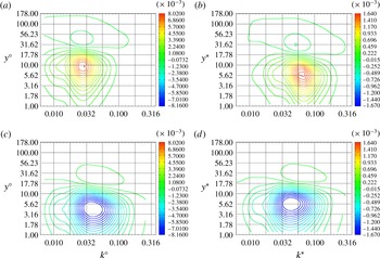
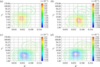
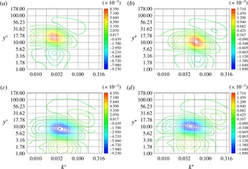
This applies to all wall-normal positions and all terms investigated by Bolotnov et al. (Reference Bolotnov, Lahey, Drew, Jansen and Oberai2010), as shown by the comparison of the two-dimensional spectra of the production in figure 8, the interplane triadic transfer in figure 9, the inplane triadic transfer in figure 10, the inplane triadic transfer in figure 10, the interplane dissipation in figure 11, the inplane dissipation in figure 12 and the viscous transfer in figure 13. In each case, both plot uses the same normalization and the colour scales are identical. For each plot, our results agree very closely with the results of Bolotnov et al. (Reference Bolotnov, Lahey, Drew, Jansen and Oberai2010). The two spectra follow the same general behaviour. They also are in a very good agreement on the spatial and spectral location of the terms. Nevertheless, there are some differences. The results of Bolotnov et al. (Reference Bolotnov, Lahey, Drew, Jansen and Oberai2010) tends to have a lower amplitude and be more spread out in wavenumber. This is the same behaviour as previously discussed for the spectral profile of production and the same remarks may apply.
4 Results
The numerical results with regard to the terms of the evolution equation of the half-trace of the velocity fluctuation correlation tensor are discussed in this section.
The energy exchanges associated with the half-trace of the velocity fluctuation correlation tensor are investigated in the spatial and spectral domains. In both cases, the analysis is carried out in two configurations as described in § 3.1: the isothermal configuration and the anisothermal configuration. In the isothermal configuration, the flow is incompressible as there is no temperature gradient. In the anisothermal configuration, the strong temperature gradient generates large variations of the fluid properties. In the spatial domain, the terms of the half-trace of the velocity fluctuation correlation tensor have been studied in the literature in the isothermal configuration (see e.g. Moser et al. Reference Moser, Kim and Mansour1999; Vreman & Kuerten Reference Vreman and Kuerten2014), but has not been documented in the anisothermal configuration. In the spectral domain, the analysis is novel in both the isothermal and anisothermal configurations with the decomposition used in this study. The spatial results in the isothermal configuration are used solely to validate the numerical method. In this section, we discuss the results in the isothermal configuration in the spectral domain and in the anisothermal configuration in both the spatial and spectral domains.
The effect of the temperature gradient on the terms of the evolution equation of the half-trace of the velocity fluctuation correlation tensor is decomposed in two separate effects. The first effect is the behaviour modification of the terms of the incompressible evolution equation, here called incompressible terms. The second effect is the addition of terms specific to flows with variable fluid properties, here called thermal terms. Each term is associated with an energy exchange, that is either a conservative energy transfer or an interaction with another part of total energy. The incompressible energy exchanges are modified by the temperature gradient both through the incompressible terms and the addition of thermal terms to their expression. Additionally, a new thermal energy exchange is added, composed only of thermal terms.
In both the spatial and spectral domains, the analysis of the energy exchanges in the anisothermal configuration first investigates the effect of the temperature gradient on the incompressible energy exchanges. Then, we investigate the contribution of the thermal terms to the energy exchanges. This analysis includes the thermal terms of the incompressible energy exchanges and of the thermal energy exchange.
4.1 Scalings
For later use, we define here the four following scalings: the constant scaling, the classical scaling, the semi-local scaling and the integral scaling. With the constant scaling, all profiles are scaled identically thus keeping the same relative behaviour as the raw profiles. The scaling uses a combination of the friction velocity
 $U_{\unicode[STIX]{x1D70F}}^{\circ }$
and the cinematic viscosity at the wall
 $\unicode[STIX]{x1D708}_{\unicode[STIX]{x1D714}}^{\circ }$
in the isothermal configuration. This scaling uses the results of the isothermal configuration even for profiles in the anisothermal case since the scaling should always be the same. The constant scaling is denoted with a superscript circle (
 $^{\circ }$
),
 $$\begin{eqnarray}\displaystyle & \displaystyle y^{\circ }=\frac{yU_{\unicode[STIX]{x1D70F}}^{\circ }}{\unicode[STIX]{x1D708}_{\unicode[STIX]{x1D714}}^{\circ }}, & \displaystyle\end{eqnarray}$$
 $$\begin{eqnarray}\displaystyle & \displaystyle k^{\circ }=\frac{k\unicode[STIX]{x1D708}_{\unicode[STIX]{x1D714}}^{\circ }}{U_{\unicode[STIX]{x1D70F}}^{\circ }}, & \displaystyle\end{eqnarray}$$
 $$\begin{eqnarray}\displaystyle & \displaystyle U^{\circ }=\frac{U}{U_{\unicode[STIX]{x1D70F}}^{\circ }}, & \displaystyle\end{eqnarray}$$
 $$\begin{eqnarray}\displaystyle & \displaystyle e^{\circ }=\frac{e}{{U_{\unicode[STIX]{x1D70F}}^{\circ }}^{2}}, & \displaystyle\end{eqnarray}$$
 $$\begin{eqnarray}\displaystyle & \displaystyle \left({\displaystyle \frac{\unicode[STIX]{x2202}e}{\unicode[STIX]{x2202}t}}\right)^{\circ }=\frac{1}{{U_{\unicode[STIX]{x1D70F}}^{\circ }}^{4}/\unicode[STIX]{x1D708}_{\unicode[STIX]{x1D714}}^{\circ }}\left({\displaystyle \frac{\unicode[STIX]{x2202}e}{\unicode[STIX]{x2202}t}}\right). & \displaystyle\end{eqnarray}$$
With the classical scaling, the profiles are scaled using the results at the same side of the channel. All quantities are scaled by a combination of the friction velocity
 $U_{\unicode[STIX]{x1D70F}}$
and the cinematic viscosity
 $\unicode[STIX]{x1D708}_{\unicode[STIX]{x1D714}}$
at the closest wall. The classical scaling is denoted with a superscript plus sign (
 $^{+}$
),
 $$\begin{eqnarray}\displaystyle & \displaystyle y^{+}=\frac{yU_{\unicode[STIX]{x1D70F}}}{\unicode[STIX]{x1D708}_{\unicode[STIX]{x1D714}}}, & \displaystyle\end{eqnarray}$$
 $$\begin{eqnarray}\displaystyle & \displaystyle k^{+}=\frac{k\unicode[STIX]{x1D708}_{\unicode[STIX]{x1D714}}}{U_{\unicode[STIX]{x1D70F}}}, & \displaystyle\end{eqnarray}$$
 $$\begin{eqnarray}\displaystyle & \displaystyle U^{+}=\frac{U}{U_{\unicode[STIX]{x1D70F}}}, & \displaystyle\end{eqnarray}$$
 $$\begin{eqnarray}\displaystyle & \displaystyle e^{+}=\frac{e}{U_{\unicode[STIX]{x1D70F}}^{2}}, & \displaystyle\end{eqnarray}$$
 $$\begin{eqnarray}\displaystyle & \displaystyle \left({\displaystyle \frac{\unicode[STIX]{x2202}e}{\unicode[STIX]{x2202}t}}\right)^{+}=\frac{1}{U_{\unicode[STIX]{x1D70F}}^{4}/\unicode[STIX]{x1D708}_{\unicode[STIX]{x1D714}}}\left({\displaystyle \frac{\unicode[STIX]{x2202}e}{\unicode[STIX]{x2202}t}}\right). & \displaystyle\end{eqnarray}$$
With the semi-local scaling, the profiles takes into account the mean local fluid properties instead of the fluid properties at the wall. The semi-local scaling is denoted with a superscript asterisk (
 $^{\ast }$
),
 $$\begin{eqnarray}\displaystyle & \displaystyle y^{\ast }=\frac{yU_{\unicode[STIX]{x1D70F}}^{\ast }}{\overline{\unicode[STIX]{x1D708}}(y)}, & \displaystyle\end{eqnarray}$$
 $$\begin{eqnarray}\displaystyle & \displaystyle k^{\ast }=\frac{k\overline{\unicode[STIX]{x1D708}}(y)}{U_{\unicode[STIX]{x1D70F}}^{\ast }}, & \displaystyle\end{eqnarray}$$
 $$\begin{eqnarray}\displaystyle & \displaystyle U^{\ast }=\frac{U}{U_{\unicode[STIX]{x1D70F}}^{\ast }}, & \displaystyle\end{eqnarray}$$
 $$\begin{eqnarray}\displaystyle & \displaystyle e^{\ast }=\frac{e}{{U_{\unicode[STIX]{x1D70F}}^{\ast }}^{2}}, & \displaystyle\end{eqnarray}$$
 $$\begin{eqnarray}\displaystyle & \displaystyle \left({\displaystyle \frac{\unicode[STIX]{x2202}e}{\unicode[STIX]{x2202}t}}\right)^{\ast }=\frac{1}{{U_{\unicode[STIX]{x1D70F}}^{\ast }}^{4}/\overline{\unicode[STIX]{x1D708}}(y)}\left({\displaystyle \frac{\unicode[STIX]{x2202}e}{\unicode[STIX]{x2202}t}}\right), & \displaystyle\end{eqnarray}$$
with,
 $$\begin{eqnarray}U_{\unicode[STIX]{x1D70F}}^{\ast }=\sqrt{\frac{\unicode[STIX]{x1D707}_{\unicode[STIX]{x1D714}}}{\overline{\unicode[STIX]{x1D70C}}(y)}\left({\displaystyle \frac{\unicode[STIX]{x2202}\overline{U}_{x}}{\unicode[STIX]{x2202}y}}\right)_{\unicode[STIX]{x1D714}}}.\end{eqnarray}$$
The semi-local scaling is part of the current paradigm of scalings for compressible wall turbulence (Trettel & Larsson Reference Trettel and Larsson2016). While it was first proposed using heuristic arguments (Rotta Reference Rotta1959; Coleman, Kim & Moser Reference Coleman, Kim and Moser1995; Huang et al. Reference Huang, Coleman and Bradshaw1995), two different mathematical frameworks were developed recently to support the validity of the semi-local scaling by Patel et al. (Reference Patel, Peeters, Boersma and Pecnik2015) and Trettel & Larsson (Reference Trettel and Larsson2016).
With the integral scaling, the profiles are scaled using an integral length scale as in Brun et al. (Reference Brun, Boiarciuc, Haberkorn and Comte2008). The integral scaling is denoted with a superscript (
 $^{B}$
),
 $$\begin{eqnarray}\displaystyle & \displaystyle y^{B}=\int _{0}^{y^{+}}\frac{\unicode[STIX]{x1D707}_{\unicode[STIX]{x1D714}}}{\overline{\unicode[STIX]{x1D707}}(y)}\,\text{d}y^{+} & \displaystyle\end{eqnarray}$$
 $$\begin{eqnarray}\displaystyle & \displaystyle U^{B}=\frac{U}{U_{\unicode[STIX]{x1D70F}}^{B}} & \displaystyle\end{eqnarray}$$
 $$\begin{eqnarray}\displaystyle & \displaystyle e^{B}=\frac{e}{{U_{\unicode[STIX]{x1D70F}}^{B}}^{2}} & \displaystyle\end{eqnarray}$$
 $$\begin{eqnarray}\displaystyle & \displaystyle \left({\displaystyle \frac{\unicode[STIX]{x2202}e}{\unicode[STIX]{x2202}t}}\right)^{B}=\frac{1}{{U_{\unicode[STIX]{x1D70F}}^{B}}^{4}/\unicode[STIX]{x1D708}_{\unicode[STIX]{x1D714}}}\left({\displaystyle \frac{\unicode[STIX]{x2202}e}{\unicode[STIX]{x2202}t}}\right), & \displaystyle\end{eqnarray}$$
with,
 $$\begin{eqnarray}U_{\unicode[STIX]{x1D70F}}^{B}=\frac{y^{B}}{y^{+}}\frac{\overline{\unicode[STIX]{x1D707}}(y)}{\unicode[STIX]{x1D707}_{\unicode[STIX]{x1D714}}}\sqrt{\frac{\unicode[STIX]{x1D70C}_{\unicode[STIX]{x1D714}}}{\overline{\unicode[STIX]{x1D70C}}(y)}}U_{\unicode[STIX]{x1D70F}}.\end{eqnarray}$$
In particular, note that the terms of the evolution equation of the half-trace of the velocity fluctuation correlation tensor are scaled by
 ${U_{\unicode[STIX]{x1D70F}}^{\circ }}^{4}/\unicode[STIX]{x1D708}_{\unicode[STIX]{x1D714}}^{\circ }$
with the constant scaling,
 ${U_{\unicode[STIX]{x1D70F}}}^{4}/\unicode[STIX]{x1D708}_{\unicode[STIX]{x1D714}}$
with the classical scaling,
 ${U_{\unicode[STIX]{x1D70F}}^{\ast }}^{4}/\overline{\unicode[STIX]{x1D708}}(y)$
with the semi-local scaling and
 ${U_{\unicode[STIX]{x1D70F}}^{B}}^{4}/\unicode[STIX]{x1D708}_{\unicode[STIX]{x1D714}}$
with the integral scaling.
We remark that the values of
 ${U_{\unicode[STIX]{x1D70F}}}^{4}/\unicode[STIX]{x1D708}_{\unicode[STIX]{x1D714}}$
at the hot and cold sides are the same within 0.5 % accuracy. The classical scaling thus does not modify the relative amplitude of the hot and cold sides. We do not see any physical reason for the equality of
 ${U_{\unicode[STIX]{x1D70F}}}^{4}/\unicode[STIX]{x1D708}_{\unicode[STIX]{x1D714}}$
at the two sides, that is of the relation
 $$\begin{eqnarray}\unicode[STIX]{x1D708}_{\unicode[STIX]{x1D714}_{1}}\left({\displaystyle \frac{\unicode[STIX]{x2202}\overline{U}_{x}}{\unicode[STIX]{x2202}y}}\right)_{\unicode[STIX]{x1D714}_{1}}^{2}=\unicode[STIX]{x1D708}_{\unicode[STIX]{x1D714}_{2}}\left({\displaystyle \frac{\unicode[STIX]{x2202}\overline{U}_{x}}{\unicode[STIX]{x2202}y}}\right)_{\unicode[STIX]{x1D714}_{2}}^{2},\end{eqnarray}$$
where the subscript
 $\unicode[STIX]{x1D714}_{1}$
denotes the value at the cold wall and the subscript
 $\unicode[STIX]{x1D714}_{2}$
the value at the hot wall. Further analyses at different friction Reynolds number and temperature ratios are required to verify the possible generality of the property.
4.2 Assessment of the amplitude of the terms
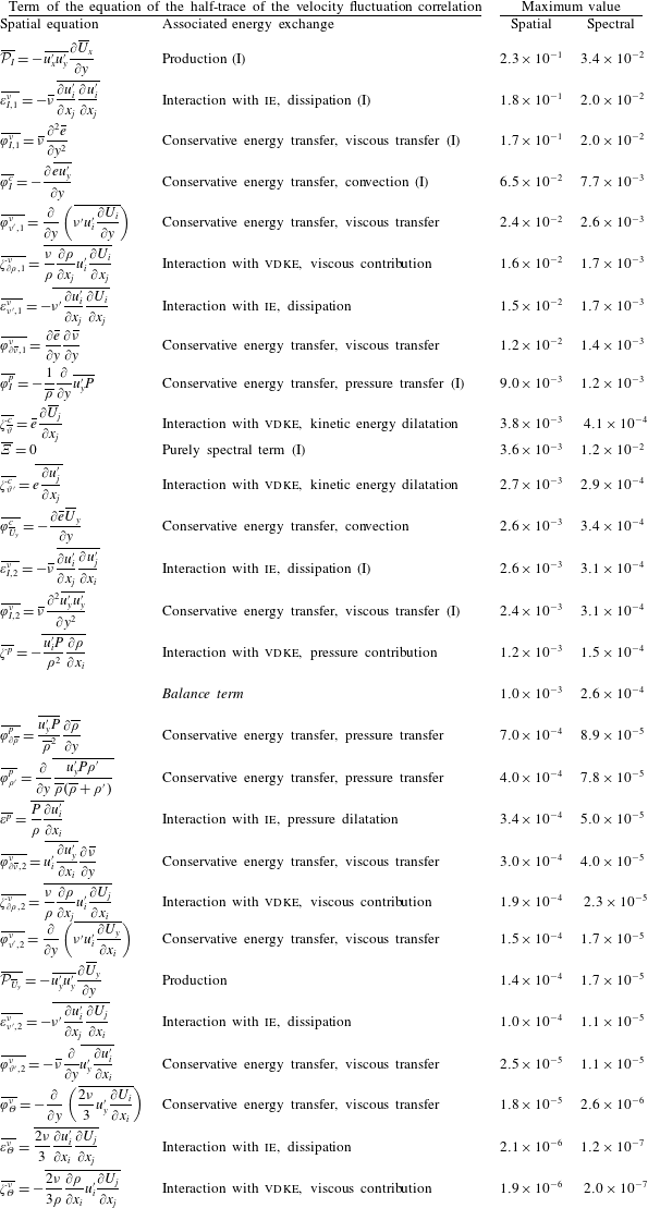
The maximum amplitude of each term of the evolution equation of the half-trace of the velocity fluctuation correlation tensor is reported in table 2. The purpose of this is twofold. First, this gives an estimate of the relative importance of each term. Second, the importance of each term compared to the balance term indicates whether the term has reliable statistics.
Maximum value of the terms of the evolution equation of the half-trace of the velocity fluctuation correlation tensor in the spatial and spectral domain. For the sake of conciseness, the expression of each term is given in the spatial domain only. The type of each term refers to the four energy exchanges associated with the half-trace of the velocity fluctuation correlation tensor according to the ternary representation: the conservative energy transfer, the interaction with internal energy (ie), the production, interaction with the other parts of kinetic energy and the interaction with variable density kinetic energy (vdke). The symbol (I) is appended to the terms that do no vanish in the incompressible case. The results are given with the classical scaling.
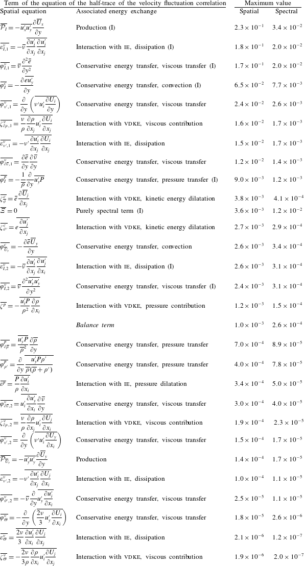
The most significant terms in the low Mach anisothermal channel flow remain the incompressible terms, namely terms that do not vanish in the incompressible case. For each energy exchange, the most important term of the decomposition is an incompressible term, with the obvious exception of the interaction with variable density kinetic energy which vanish in the incompressible case. The only incompressible terms that have a very low maximum amplitude are the two terms
 $\overline{\unicode[STIX]{x1D700}_{I,2}^{\unicode[STIX]{x1D708}}}$
and
 $\overline{\unicode[STIX]{x1D711}_{I,2}^{\unicode[STIX]{x1D708}}}$
, which cancel each other out in the incompressible case. The purely spectral term is found to be a major part of the energy exchanges in the spectral domain.
The amplitudes of the thermal terms do not follow those of the associated incompressible terms. For instance, while the incompressible production is the term with the highest amplitude, the thermal production is one of the smallest terms. Instead, it depends primarily on the underlying physical origin of the terms. The most significant thermal terms are terms associated with the viscous shear stress, and more specifically the part associated with the product with the velocity gradient. Though, they differ in the energy exchange they are associated with (conservative energy transfer, interaction with internal energy or with variable density kinetic energy) and the source of their thermal character (fluctuation of the viscosity, variation of the mean viscosity or of the density). With regard to the terms associated with the other parts of the viscous shear stress, the terms associated with the product with the transpose of the velocity gradient are very small compared to the terms associated with the product with the velocity gradient. The terms associated with the product with the velocity divergence are the smallest terms of all. This is only true for the viscous terms as the kinetic energy dilatation correlation and to a lesser extent the pressure dilatation correlation have larger amplitude.
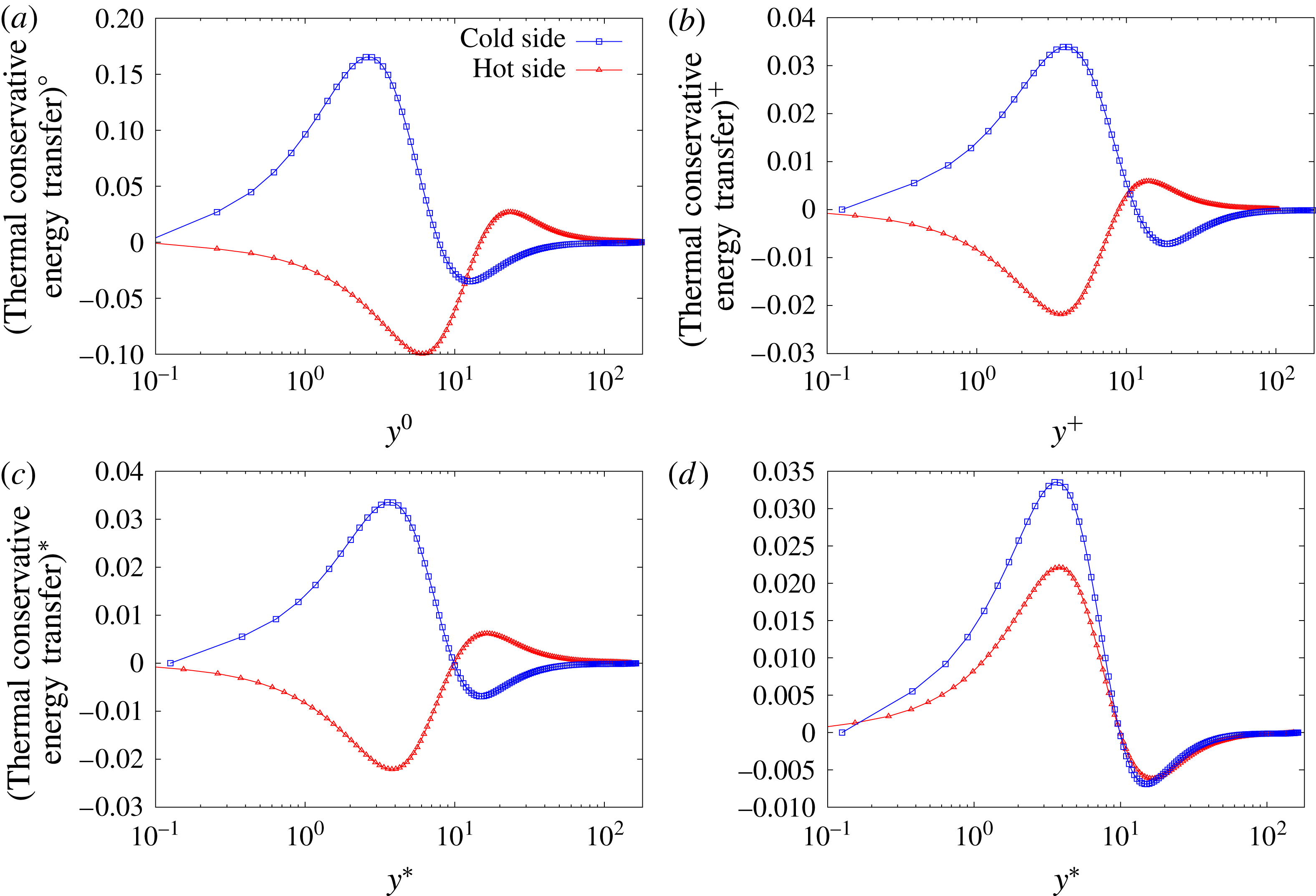
Hence, the effect of the thermal terms with regard to the energy exchanges is the largest on the conservative energy transfer and the interaction with internal energy. The two most significant terms of the thermal conservative energy transfer
 $\overline{\unicode[STIX]{x1D711}_{\unicode[STIX]{x1D6E4}}}$
are
 $\overline{\unicode[STIX]{x1D711}_{\unicode[STIX]{x1D708}^{\prime },1}^{\unicode[STIX]{x1D708}}}$
and
 $\overline{\unicode[STIX]{x1D711}_{\unicode[STIX]{x2202}\overline{\unicode[STIX]{x1D708}},1}^{\unicode[STIX]{x1D708}}}$
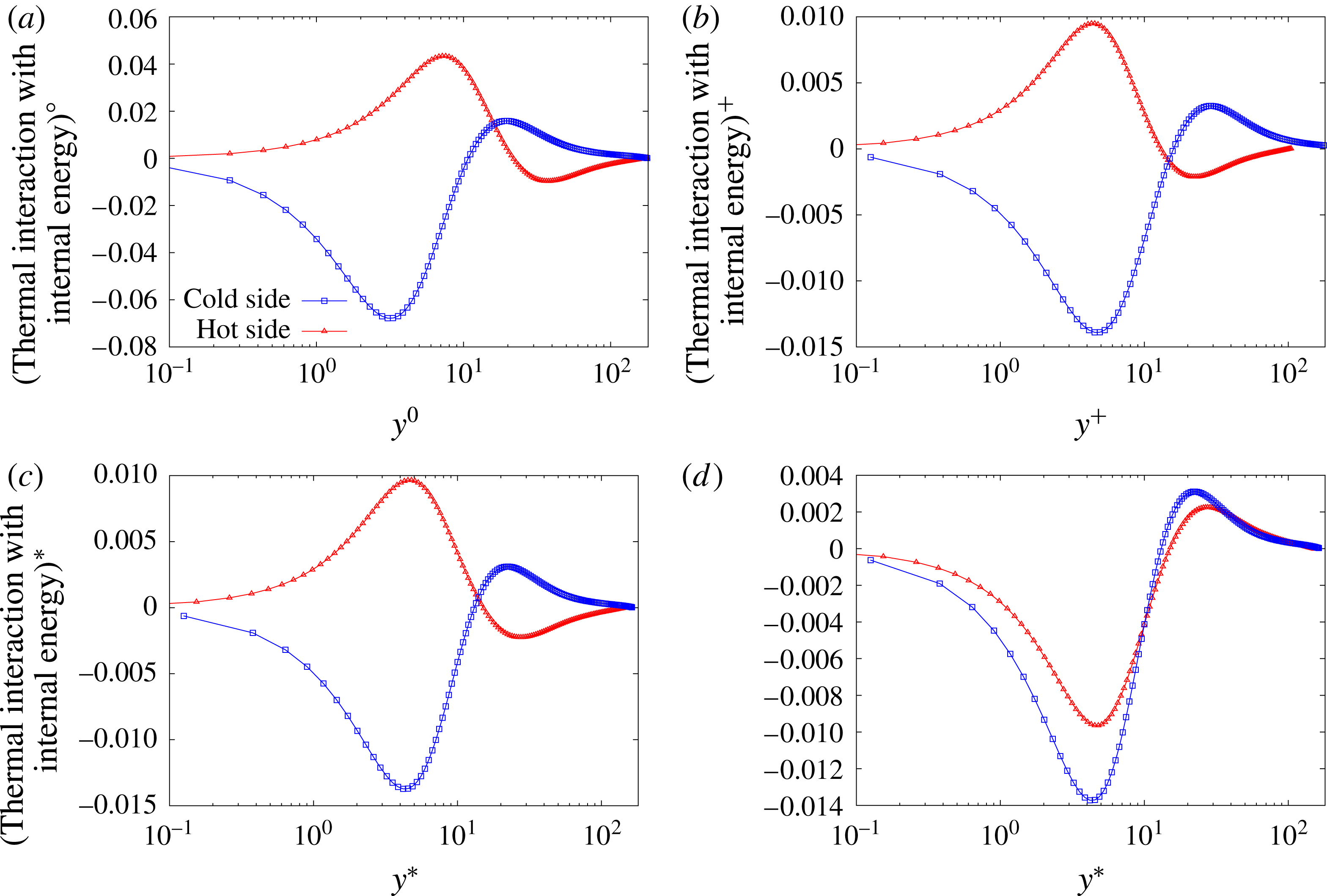
, both part of the thermal viscous transfer. In the thermal interaction with internal energy
 $\overline{\unicode[STIX]{x1D700}_{\unicode[STIX]{x1D6E4}}}$
, the term
 $\overline{\unicode[STIX]{x1D700}_{\unicode[STIX]{x1D708}^{\prime },1}^{\unicode[STIX]{x1D708}}}$
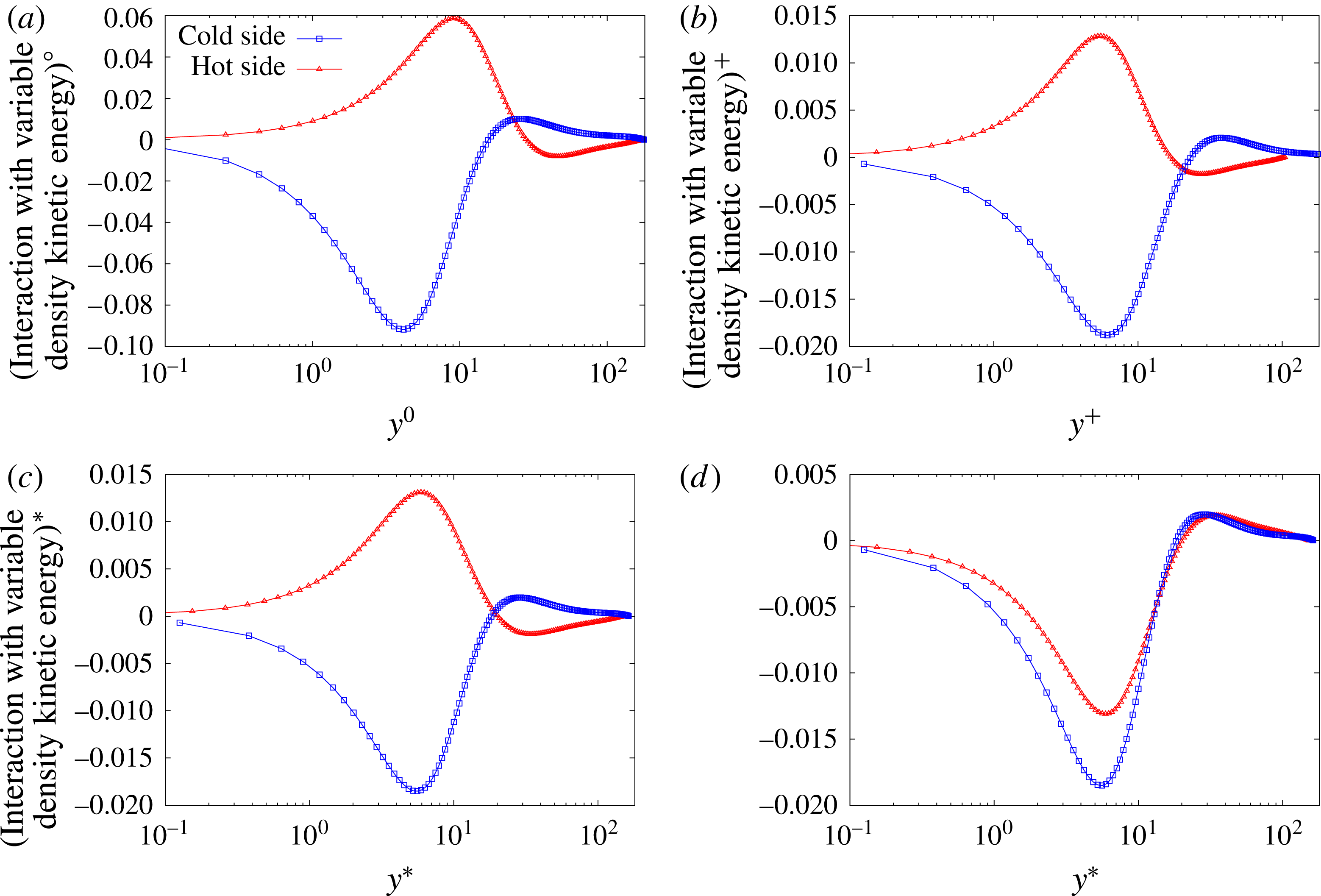
predominates. The additional energy exchange with variable density kinetic energy
 $\overline{\unicode[STIX]{x1D701}}$
is substantial. It acts primarily through its viscous contribution and secondly through the kinetic energy dilatation correlation. For the three interactions, the pressure contribution is not significant. Note however that the data provided in the table are mute towards the local importance of the terms, which may be larger or lower than what the maximum amplitude make it appears to be.
For the purpose of this paper, a term is considered statistically reliable if its maximum amplitude is at least ten times larger than the maximum amplitude of the kinetic energy balance. This leaves the eight following statistically reliable terms:
-
(i)
$\overline{{\mathcal{P}}_{I}}$
, the incompressible production, -
(ii)
$\overline{\unicode[STIX]{x1D700}_{I,1}^{\unicode[STIX]{x1D708}}}$
, a part of the incompressible dissipation, -
(iii)
$\overline{\unicode[STIX]{x1D711}_{I,1}^{\unicode[STIX]{x1D708}}}$
, a part of the incompressible viscous transfer, -
(iv)
$\overline{\unicode[STIX]{x1D711}_{I}^{c}}$
, the convection by turbulent motion, -
(v)
$\overline{\unicode[STIX]{x1D711}_{\unicode[STIX]{x1D708}^{\prime },1}^{\unicode[STIX]{x1D708}}}$
, a part of viscosity fluctuation viscous transfer, -
(vi)
$\overline{\unicode[STIX]{x1D701}_{\unicode[STIX]{x2202}\unicode[STIX]{x1D70C},1}^{\unicode[STIX]{x1D708}}}$
, a part of the density variation viscous interaction with variable density kinetic energy, -
(vii)
$\overline{\unicode[STIX]{x1D700}_{\unicode[STIX]{x1D708}^{\prime },1}^{\unicode[STIX]{x1D708}}}$
, a part of the viscosity fluctuation dissipation, -
(viii)
$\overline{\unicode[STIX]{x1D711}_{\unicode[STIX]{x2202}\overline{\unicode[STIX]{x1D708}},1}^{\unicode[STIX]{x1D708}}}$
, a part of the mean viscosity variation viscous transfer.


In the following, the behaviour of those eight terms is analysed. The remaining 18 terms are not discussed individually as their amplitude is too low to ensure that their profile is correctly described. In particular, the pressure transfer and the pressure contribution to the interaction with variable density kinetic energy and the interaction with internal energy will not be studied.
Production, total
 $\overline{{\mathcal{P}}}$
and incompressible
 $\overline{{\mathcal{P}}_{I}}$
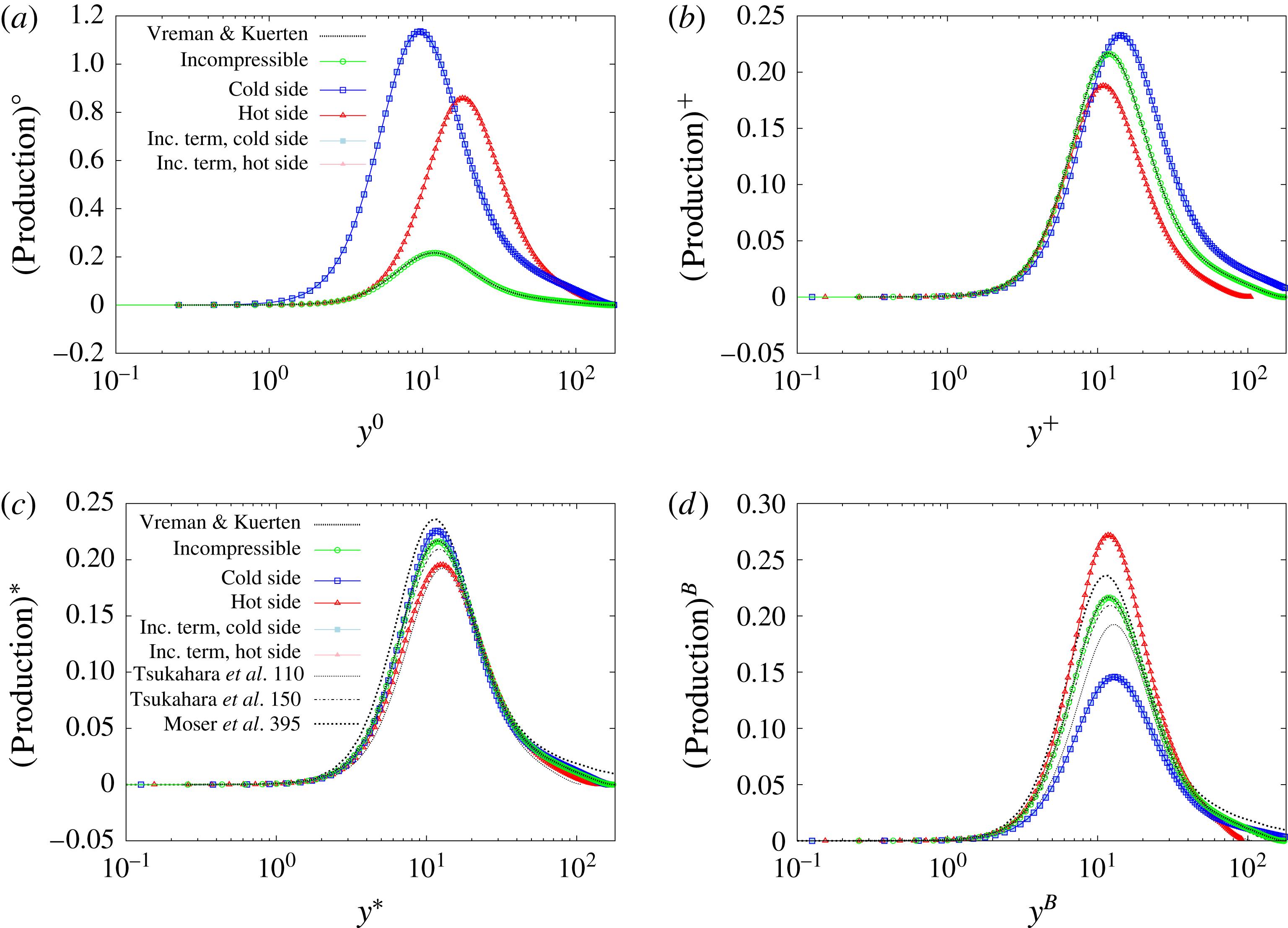
: (a) constant scaling; (b) classical scaling; (c) semi-local scaling; (d) integral scaling (Brun et al.
Reference Brun, Boiarciuc, Haberkorn and Comte2008).

Conservative energy transfer, total
 $\overline{\unicode[STIX]{x1D711}}$
and incompressible
 $\overline{\unicode[STIX]{x1D711}_{I}}$
: (a) constant scaling; (b) classical scaling; (c) semi-local scaling; (d) integral scaling (Brun et al.
Reference Brun, Boiarciuc, Haberkorn and Comte2008).

Interaction with internal energy, total
 $\overline{\unicode[STIX]{x1D700}}$
and incompressible
 $\overline{\unicode[STIX]{x1D700}_{I}^{\unicode[STIX]{x1D708}}}$
: (a) constant scaling; (b) classical scaling; (c) semi-local scaling; (d) integral scaling (Brun et al.
Reference Brun, Boiarciuc, Haberkorn and Comte2008).

4.3 Results in the spatial domain
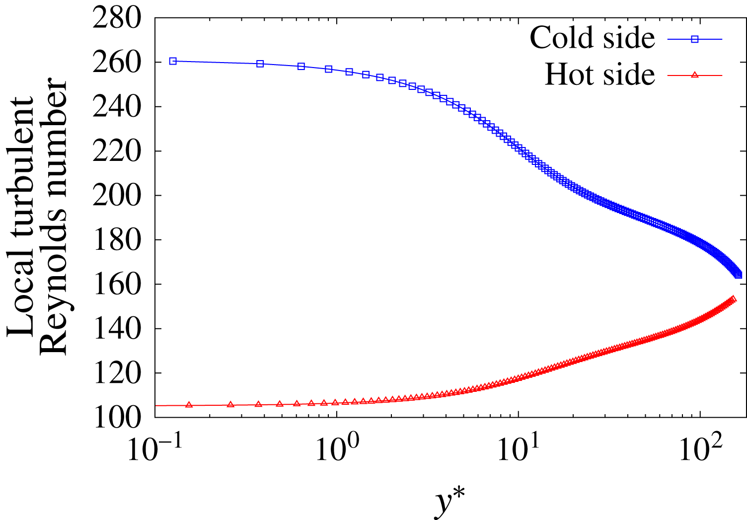
In this section, we investigate the energy exchanges associated with the half-trace of the velocity fluctuation correlation tensor in the spatial domain. The analysis is carried out in three steps. First, we study the total effect of the temperature gradient on the incompressible energy exchanges, through the combined effect of the modification of the behaviour of the incompressible terms and the addition of thermal terms. In particular, we study the effect of the Reynolds number variations across the channel. Then, we focus on the contribution of the modification of the incompressible terms to the alteration of the incompressible energy exchanges. Finally, we investigate the profiles of the thermal terms.
4.3.1 Profiles of the incompressible energy exchanges in the anisothermal configuration
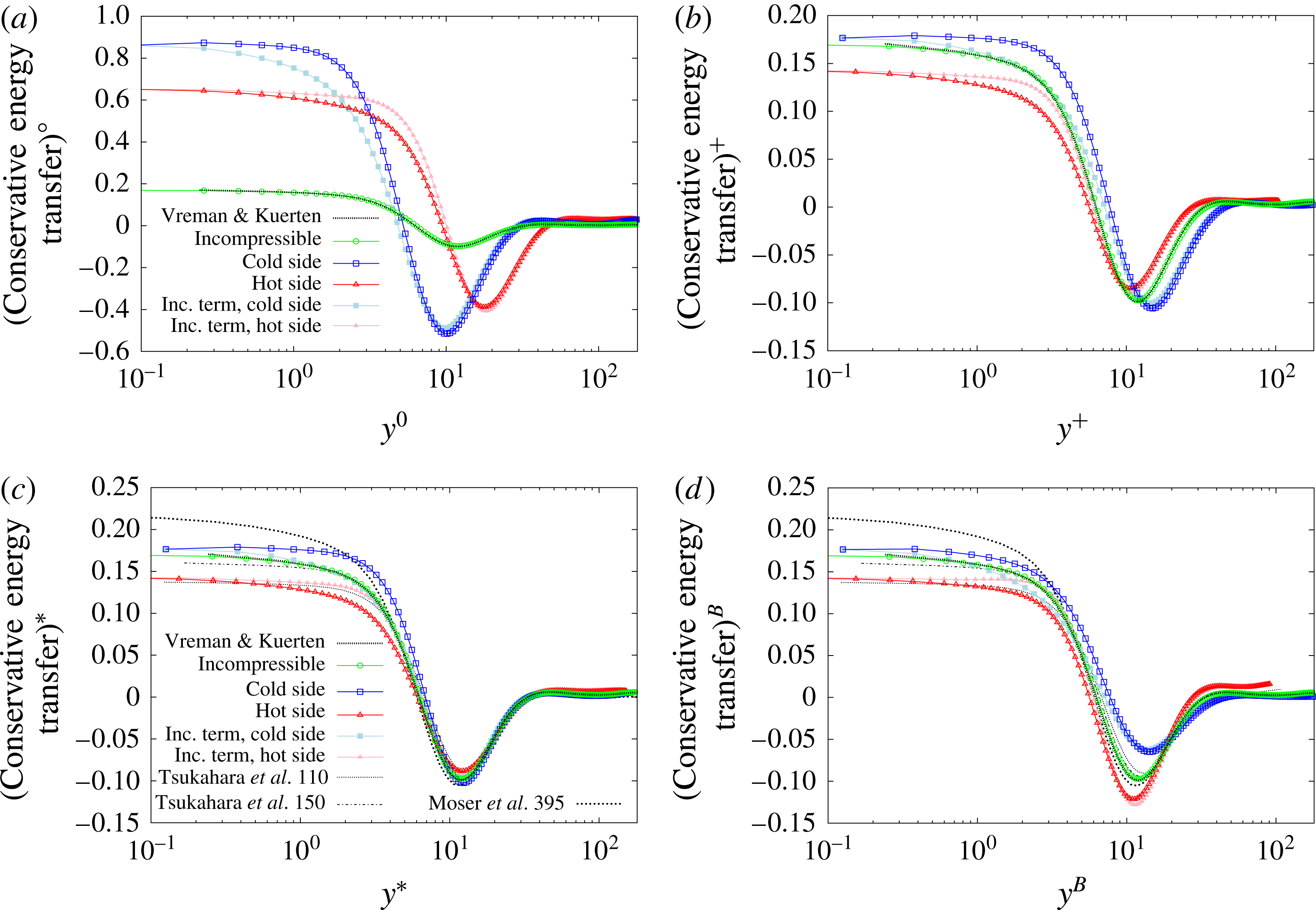
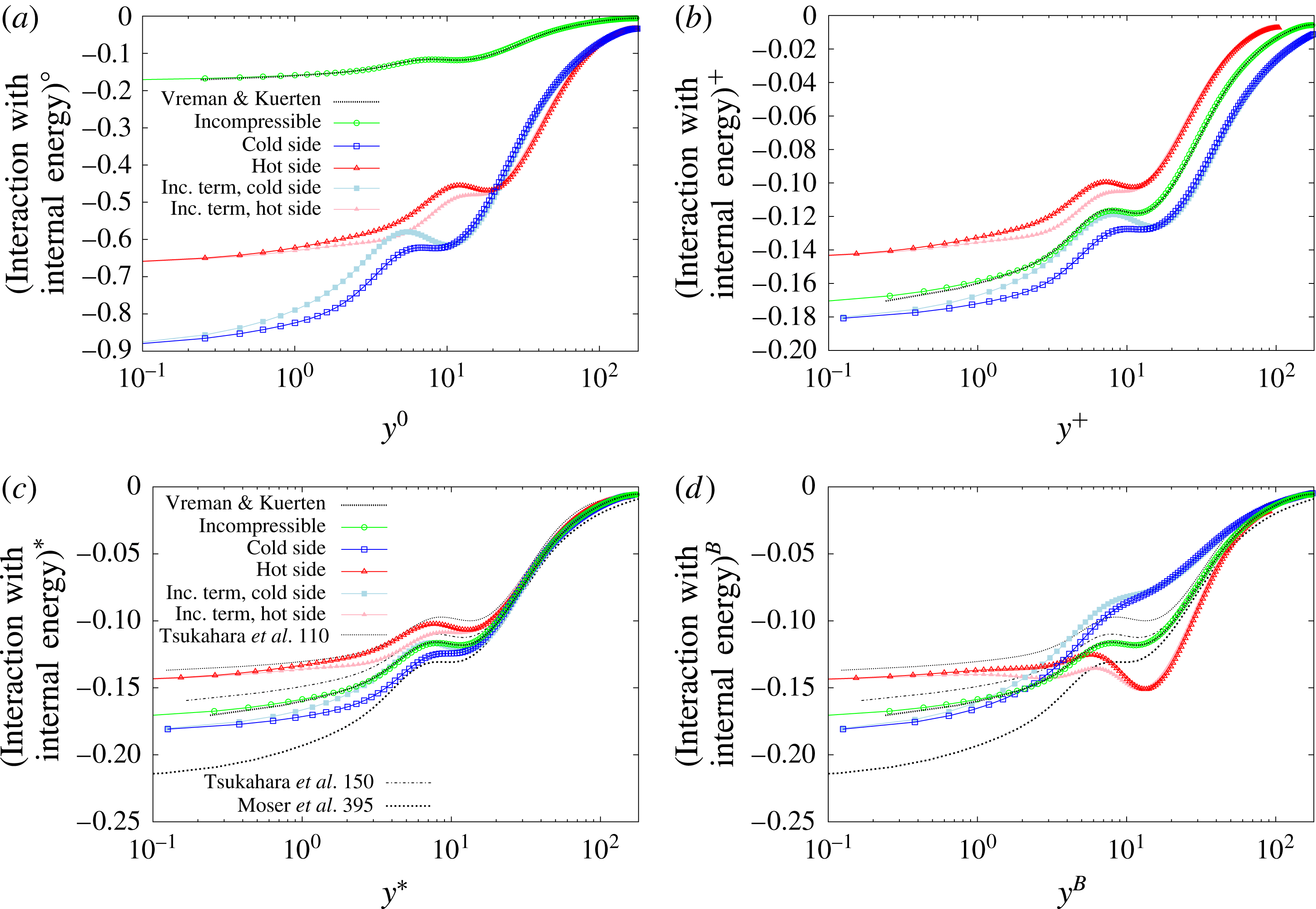
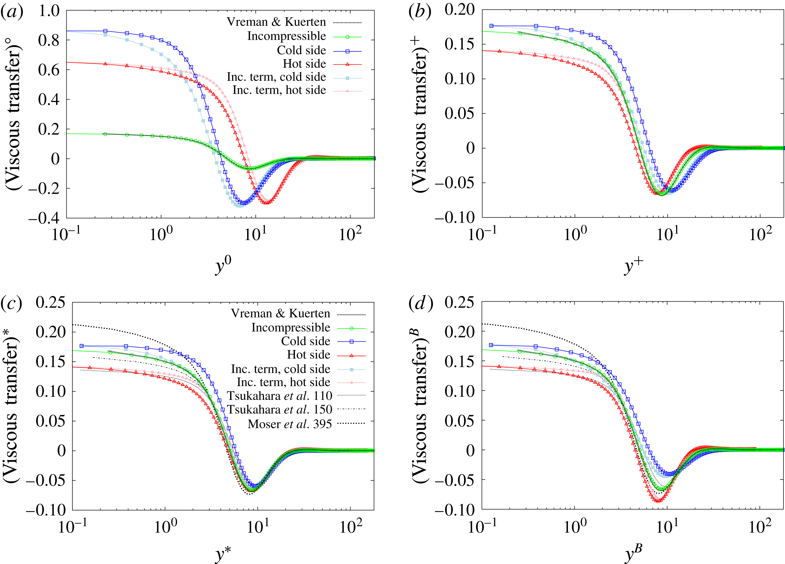
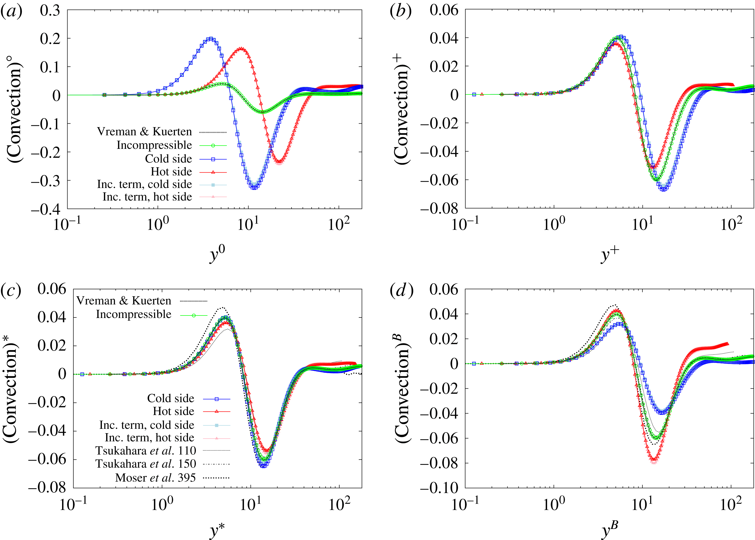
The four energy exchanges associated with the half-trace of the velocity fluctuation correlation tensor are the production, the conservative energy transfer, the interaction with variable density kinetic energy and the interaction with internal energy. The production represented in figure 14, the conservative energy transfer in figure 15 and the interaction with internal energy in figure 16. The interaction with variable density kinetic energy is discussed later since, as a thermal energy exchange, its behaviour is particular. We also provide the profile of the relevant parts of each term. The viscous transfer is given in figure 17 and the turbulent transfer in figure 18. The pressure transfer is not discussed because it is not statistically reliable in the anisothermal configuration. The dissipation is given by the profile of the interaction with internal energy, since the pressure dilatation is negligible.
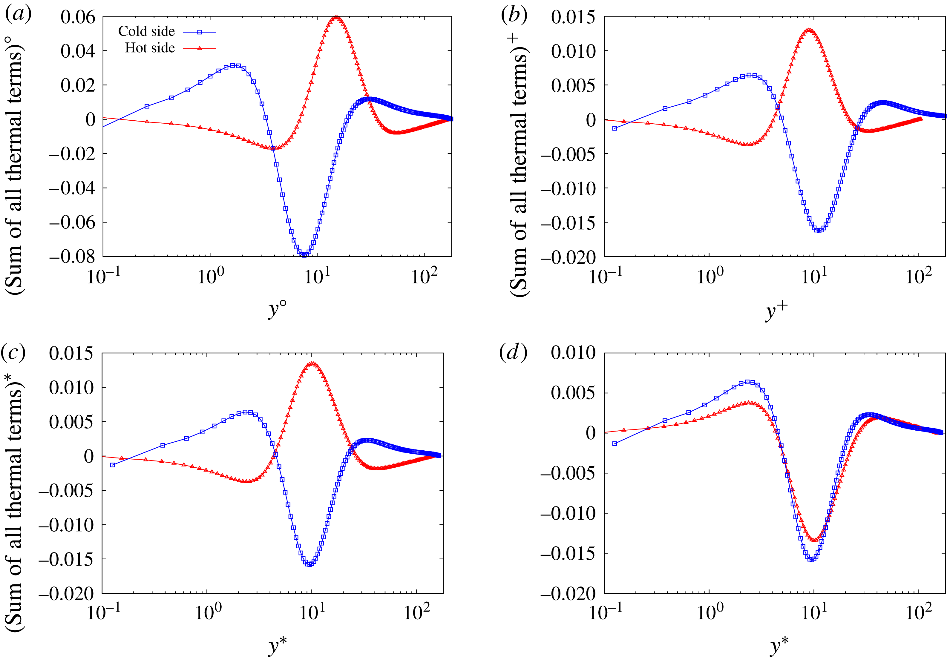
For each term, the profiles at the hot and cold sides are compared to each other and to the corresponding profile in the isothermal configuration. The results are given with the constant scaling, the classical scaling, the semi-local scaling and the integral scaling. The three scalings show an asymmetry between the hot and cold profiles, though of different nature. Some generalities are found in the manner in which the temperature gradient manifests itself as summarized in the following.
Viscous transfer (part of the conservative energy transfer), total
 $\overline{\unicode[STIX]{x1D711}^{\unicode[STIX]{x1D708}}}$
and incompressible
 $\overline{\unicode[STIX]{x1D711}_{I}^{\unicode[STIX]{x1D708}}}$
: (a) constant scaling; (b) classical scaling; (c) semi-local scaling; (d) integral scaling (Brun et al.
Reference Brun, Boiarciuc, Haberkorn and Comte2008).

Convection (part of the conservative energy transfer), total
 $\overline{\unicode[STIX]{x1D711}^{c}}$
and incompressible
 $\overline{\unicode[STIX]{x1D711}_{I}^{c}}$
: (a) constant scaling; (b) classical scaling; (c) semi-local scaling; (d) integral scaling (Brun et al.
Reference Brun, Boiarciuc, Haberkorn and Comte2008).

The constant scaling shows the effect of the temperature gradient when not correcting the friction velocity and viscosity differences between the isothermal and anisothermal case. The general behaviour of the profiles is never drastically modified. However, the amplitudes in absolute value are increased considerably at the hot and cold side compared to the isothermal results. The amplitudes at the cold side are larger than the amplitudes at the hot side. Meanwhile, the positions of the local or global extrema are shifted closer to the wall at the cold side compared to the isothermal profile and closer to the centre of the channel at the hot side. Since the wall-normal coordinate axis is logarithmic, this shift comes with an increase of the spatial range of the term at the hot side and a decrease at the cold side. In particular, the effect of the amplitude and spatial extent modification offset each other for the production, such that the total integrated production is the same at the hot and cold side. Within 1 % error, this remark may also be applied to the interaction with internal energy.
The classical scaling shows the effect of the temperature gradient when scaled by the friction velocity and the viscosity at the wall. With the classical scaling, the anisothermal profiles have the same order of magnitude as the isothermal profile. This proves that most of the amplitude differences seen with the constant scaling are due to the increased friction velocity on the anisothermal configuration. The scaled amplitude at the cold side is increased compared to the isothermal profile and decreased at the hot side. We recall that the classical scaling has no effect on the relative amplitude of the terms at the hot and cold side since the value of
 $U_{\unicode[STIX]{x1D70F}}^{4}/\unicode[STIX]{x1D708}_{\unicode[STIX]{x1D714}}$
is the same at both sides of the channel. In other words, the classical scaling successfully explains the differences between the isothermal amplitudes and the anisothermal amplitudes but is silent towards the difference between the hot and cold sides. The relative position of the local or global extrema of the hot, cold and isothermal profiles are swapped by the classical scaling. Now, the extrema are seen shifted closer to the wall in wall units at the hot side compared to the isothermal profile and closer to the centre of the channel at the cold side. A good explanation is that the classical scaling takes into account the viscosity at the wall thus overcorrects the position closer to the centre of the channel where the viscosity is similar at both sides of the channel.
To address this, the semi-local scaling takes into account the mean local variations of the fluid properties. With the semi-local scaling, there is no position differences between the hot, cold and isothermal profiles. This result shows the physical relevance of the semi-local scaling, which is able to explain the positional shift of the hot and cold profiles compared to the isothermal profile. However, the amplitude differences are not modified.
A possible explanation of these amplitude differences could be a Reynolds number effect, that is the local variations of the friction Reynolds number across the channel between the hot and cold sides. Indeed, the temperature gradient creates variations of the local friction Reynolds number (figure 19), that we define as
 $U_{\unicode[STIX]{x1D70F}}^{\ast }(y)h/\overline{\unicode[STIX]{x1D708}}(y)$
following the semi-local scaling. The local friction Reynolds number spans between 107 at the hot wall and 260 at the cold wall. Within this Reynolds number range, the scaled isothermal profiles depend on the Reynolds number. This makes the semi-local scaling harder to interpret, as it would prevent the hot and cold profiles to collapse. To study the Reynolds number effect, we compare the effect of the temperature gradient to the effect of Reynolds number variations in the isothermal configuration. We use to this intent the data of Tsukahara et al. (Reference Tsukahara, Seki, Kawamura and Tochio2005) at the friction Reynolds numbers 110 and 150, the isothermal results at
 $Re_{\unicode[STIX]{x1D70F}}=180$
and the data of Moser et al. (Reference Moser, Kim and Mansour1999) at
 $Re_{\unicode[STIX]{x1D70F}}=395$
(considering the lack of available data between 180 and 395).
The semi-locally scaled profiles of production (figure 14 c) follow very closely a Reynolds number effect. We use the empirical relation between the maximum of production and the friction Reynolds number of Laadhari (Reference Laadhari2002) to compute the peak of production in the isothermal configuration associated with the friction Reynolds number of the peak of production in the anisothermal configuration (around 121 at the hot side and 215 at the cold side). The results agree within 1 % accuracy to the anisothermal results. Therefore, we can conclude that the effect of the temperature gradient on production is to a very large extent a Reynolds number effect. A mathematical argument supporting this fact can be inferred from the mean streamwise momentum balance, which may be rewritten with the semi-local scaling as
 $$\begin{eqnarray}\overline{u_{x}^{\prime \ast }u_{y}^{\prime \ast }}+{\displaystyle \frac{\unicode[STIX]{x2202}\overline{U}_{x}^{\ast }}{\unicode[STIX]{x2202}y^{\ast }}}=\left(1-\frac{y^{\ast }}{Re_{\unicode[STIX]{x1D70F}}^{\ast }}\right),\end{eqnarray}$$
assuming that
 $\overline{\unicode[STIX]{x1D70C}u_{x}^{\prime }u_{y}^{\prime }}\approx \overline{\unicode[STIX]{x1D70C}}\overline{u_{x}^{\prime }u_{y}^{\prime }}$
and
 $\overline{\unicode[STIX]{x1D707}(\unicode[STIX]{x2202}U_{x}/\unicode[STIX]{x2202}y)}\approx \overline{\unicode[STIX]{x1D707}}(\unicode[STIX]{x2202}\overline{U}_{x}/\unicode[STIX]{x2202}y)$
. The semi-locally scaled incompressible production
 $\overline{{\mathcal{P}}_{I}}^{\ast }$
is thus equal to
 $$\begin{eqnarray}\overline{{\mathcal{P}}_{I}}^{\ast }=-\overline{u_{x}^{\prime \ast }u_{y}^{\prime \ast }}{\displaystyle \frac{\unicode[STIX]{x2202}\overline{U}_{x}^{\ast }}{\unicode[STIX]{x2202}y^{\ast }}}=\left({\displaystyle \frac{\unicode[STIX]{x2202}\overline{U}_{x}^{\ast }}{\unicode[STIX]{x2202}y^{\ast }}}\right)^{2}-{\displaystyle \frac{\unicode[STIX]{x2202}\overline{U}_{x}^{\ast }}{\unicode[STIX]{x2202}y^{\ast }}}\left(1-\frac{y^{\ast }}{Re_{\unicode[STIX]{x1D70F}}^{\ast }}\right).\end{eqnarray}$$
This expression is identical to the expression of the production in the incompressible case with the semi-local scaling substituting the classical scaling, hinting that the semi-local scaling is an appropriate scaling for the production in the variable property case.
While the effect of the temperature gradient on the interaction with internal energy (figure 16
c), the viscous transfer (figure 17
c) and the convection (figure 18
c) is also in a large part due to a Reynolds number effect, this explanation is not sufficient to explain the effect of the temperature gradient on these terms. The value of the interaction with internal energy (figure 16
c) at the hot wall is comprised between the value at the wall in the isothermal configuration at
 $Re_{\unicode[STIX]{x1D70F}}=110$
and
 $Re_{\unicode[STIX]{x1D70F}}=150$
, despite being associated with a friction Reynolds number of 107. The semi-locally scaled profile of the viscous transfer (figure 17
c) deviates noticeably from all isothermal profiles from
 $y^{\ast }=10$
to the wall. In particular, while the semi-local profiles of the viscous transfer in the four isothermal configurations (
 $Re_{\unicode[STIX]{x1D70F}}=110$
, 150, 180, 395) pass through the same point at
 $y^{\ast }=3.5$
, the hot and cold anisothermal profiles deviate from this point significantly. The difference amounts to 20 % of the maximum value of the viscous transfer throughout the channel. The semi-locally scaled hot and cold profiles of the convection (figure 18
c) are farther from the isothermal profiles at the negative extremum than at the positive extremum, closer from the wall, which is the opposite of what a Reynolds number effect would imply. The effect of the temperature gradient is from these simple observations proven inconsistent with a sole Reynolds number effect. This shows that there is an additional effect that is not taken into account by the semi-local scaling and a Reynolds number effect. This effect is related to the variations of the fluid properties since it is the only new physical phenomenon in the anisothermal channel compared to the isothermal simulation. Judging from the failure of the semi-local scaling, based on the mean local value of the fluid properties, we may presume that the mean local value of the fluid properties do not explain the entirety of the effect of the temperature gradient. It may thus be necessary to take into account the fluctuations of the fluid properties to explain this effect. This is consistent with the previous study of Serra et al. (Reference Serra, Toutant, Bataille and Zhou2012b
) which showed this effect through the analysis of the isotropic component of the velocity fluctuation correlation tensor, out of which the half-trace is governed by the energy exchanges studied here.
The integral scaling is another approach to scale the profile using the mean fluid properties. The integral scaling significantly reduces the position asymmetry of the classical scaling for the production (figure 14 d). However, the scaling overcorrects the amplitude difference between the hot and cold sides and swaps their positions. The amplitude difference with the integral scaling is thus no longer consistent with a Reynolds number effect. Moreover, the integral scaling gives very unsatisfying results for the terms with non-zero value at the wall, in particular the interaction with internal energy (figure 16 d), since the ordering of the profiles at the wall is not changed. Since the integral scaling appears less appropriate, this scaling will not be discussed further in the remaining part of the paper.
Local friction Reynolds number
 $(U_{\unicode[STIX]{x1D70F}}^{\ast }h/\overline{\unicode[STIX]{x1D708}}(y))$
as a function of the distance to the wall with the semi-local scaling.

All in all, the effect of the temperature gradient on the profiles at the hot and cold sides is characterized by a twofold asymmetry. The asymmetry in the position of the extrema is explained by the mean local variations of the fluid properties. The asymmetry in the amplitudes is in part due to the local variations of the friction Reynolds number and in part due to the local fluctuations of the fluid properties.
4.3.2 Profiles of the incompressible terms in the anisothermal configuration
The effect of the temperature gradient on the profiles takes place both through the addition of thermal terms to the energy exchanges and the alteration of the profile of the incompressible terms. To assess the two phenomena, the set of figures 14–18 provides a comparison of the total energy exchanges to their incompressible part, that we recall are formally identical to the terms in the incompressible case.
In agreements with the conclusions of the analysis of the maximum amplitude of the terms in § 4.2, the production and the convection are not modified significantly by the addition of the corresponding thermal terms. However, the profiles of the interaction with internal energy, the viscous transfer and hence the conservative energy transfer are noticeably modified. With semi-local scaling, the changes are restricted to an area that arises very near to the wall and ends around
 $y^{\ast }=20$
. The scaled profile of the incompressible terms are much closer to the isothermal profile than the total term. The addition of the thermal terms separates the three profiles more clearly, moving the hot and cold profiles further away from each other and from the isothermal profile. In other words, taking into account only the incompressible terms leads to results closer to the isothermal profile than the true anisothermal profiles.
While the hot and cold profiles of the viscous transfer have a different behaviour than the isothermal profiles, the hot and cold profiles of the incompressible viscous transfer are more similar (figure 17
c). In particular, the hot and cold profiles of the incompressible viscous transfer pass through the point at
 $y^{\ast }=3.5$
as the profiles of the viscous transfer in the four isothermal configurations (
 $Re_{\unicode[STIX]{x1D70F}}=110$
, 150, 180, 395). At the hot side, the profile of the incompressible term is in line with a Reynolds number effect. The difference between the incompressible term and the total term thus represents the more complex interaction between temperature and turbulence.
4.3.3 Profiles of the thermal terms in the anisothermal configuration
We study here the thermal terms of the energy exchanges. This includes the thermal terms of the production, of the conservative energy transfer and of the interaction with internal energy and the total profile of the interaction with variable density kinetic energy since this energy exchange does not have an incompressible part. The thermal conservative energy transfer is represented in figure 20, the interaction with variable density kinetic energy in figure 21 and the thermal interaction with internal energy in figure 22. The behaviour of the thermal production is not discussed as its amplitude was found too low.
Thermal conservative energy transfer
 $\overline{\unicode[STIX]{x1D711}_{\unicode[STIX]{x1D6E4}}}$
: (a) constant scaling; (b) classical scaling; (c) semi-local scaling; (d) semi-local scaling, hot side inverted.

Interaction with variable density kinetic energy
 $\overline{\unicode[STIX]{x1D701}}$
: (a) constant scaling; (b) classical scaling; (c) semi-local scaling; (d) semi-local scaling, hot side inverted.

Thermal interaction with internal energy
 $\overline{\unicode[STIX]{x1D700}_{\unicode[STIX]{x1D6E4}}}$
: (a) constant scaling; (b) classical scaling; (c) semi-local scaling; (d) semi-local scaling, hot side inverted.

The three profiles share an interesting characteristic unknown to any of the incompressible terms. The profile at the hot and cold sides are of opposite signs. For most terms, the sign inversion can be understood from their mathematical expression. For instance,
 $\unicode[STIX]{x2202}_{y}(\overline{\unicode[STIX]{x1D708}^{\prime }u_{x}^{\prime }}\unicode[STIX]{x2202}_{y}\overline{U}_{x})$
, the leading term of the thermal conservative energy transfer undergoes a sign inversion as both
 $\overline{\unicode[STIX]{x1D708}^{\prime }u_{x}^{\prime }}$
and
 $\unicode[STIX]{x2202}_{y}\overline{U}_{x}$
undergo a sign inversion, which implies that the derivative of their product also does. Because of the sign inversion, we give, in addition to the profiles with the three scalings, the profile with the semi-local scaling with sign of the term at the hot side inverted. This allows a more convenient comparison of the hot and cold profiles when ignoring the sign difference.
The shape of the three thermal terms is similar. This is rather unexpected as the three terms are related to different energy exchanges and have different associated incompressible profiles. Besides, the interaction with variable density kinetic energy is interpreted as a new interaction whereas the thermal interaction with internal energy and the thermal conservative energy transfer are seen as the thermal part of a larger energy exchange. The hot and cold profiles both tend to zero at the wall and at the centre of the channel. Between these two points, both profiles have two extrema, one positive and one negative. The first extremum has a larger amplitude than the second extremum but the second extremum has a larger spatial range. In the thermal conservative energy transfer (figure 20), the two extrema have the same integral. This term transfers the energy from the extremum close to the wall towards the centre of the channel at the hot side, and conversely towards the wall at the cold side. On the other hand, the first extremum has a smaller integral than the second extremum for the thermal interaction with internal energy (figure 22). The effect of this term is an energy loss at the extremum close to the wall at the cold side and a gain closer to the centre of the channel at the cold side, and vice versa at the hot side. This can be thought of as a pseudo-transfer in the opposite direction to the thermal conservative energy transfer. However, this effect is accompanied by a net energy gain at the cold side and loss at the hot side. The same remark may be applied to the interaction with variable density kinetic energy (figure 21), but the transfer occurs in the opposite direction. The amplitude of the extrema is always larger at the cold side than at the hot side, and to a greater extent for the first extremum than for the second extremum. As for the incompressible energy exchanges, the spatial extent of the term is at the same time larger at the hot side compared to the cold side. As just previously noted, the significant part of the thermal terms is limited to an area that excludes the near vicinity of the wall and the centre of the channel. This can be explained as the velocity and temperature fluctuations are zero at the wall and the temperature gradient is low at the centre of the channel.
Sum of all thermal terms
 $\overline{\unicode[STIX]{x1D711}_{\unicode[STIX]{x1D6E4}}}+\overline{\unicode[STIX]{x1D701}}+\overline{\unicode[STIX]{x1D700}_{\unicode[STIX]{x1D6E4}}}$
: (a) constant scaling; (b) classical scaling; (c) semi-local scaling; (d) semi-local scaling, hot side inverted.

The signs of the extrema are the same for the two non-conservative thermal terms, and are of opposite signs for the thermal conservative energy transfer. Hence, the sum of the non-conservative terms and the sum of the conservative terms are of opposite signs. With regard to the total energy exchanges, the sum of the non-conservative terms is equal to the opposite of the conservative energy transfer. We may wonder if this property holds for the thermal terms as the thermal conservative and non-conservative terms may interact with each other only or also with the incompressible terms. To answer this question, the sum of all thermal terms is represented in figure 23. The profile is of the same order of magnitude as the thermal terms, proving that the thermal terms do not cancel out. It is composed of three extrema where, like the individual term, the profiles at the hot and cold side are of opposite sign. The integral of the positive extrema is larger than the integral of the negative extrema at both the hot and cold sides, resulting in a net energy gain overall.
The profiles of the thermal terms are modified by the classical scaling and the semi-local scaling in a similar way to the terms that do not vanish in the incompressible case. With the constant scaling, an extremum is always closer to the wall at the cold side than at the hot side. The classical scaling reduces the position differences between the hot and cold side, and swaps their relative position. Indeed, by contrast with the constant scaling, an extremum is always closer to the wall in wall units at the hot side than at the cold side. The difference is very slight for the first extremum, but larger for the second extremum. This is in agreement with the proposed interpretation of this result given in the previous section.
With the semi-local scaling, there is no position differences between the extrema of kinetic energy gain/loss at the hot and cold sides. Additionally, the areas where the hot and cold profiles are of the same sign are removed. Therefore, any kinetic energy loss coincides with a kinetic energy gain at the same position at the other side of the channel. The semi-locally scaled hot and cold profiles can thus be considered to always be of opposite sign and completely symmetric if not for the amplitude differences, which are left largely unchanged. This shows that the amplitude difference cannot be solely explained by the mean local variations of the fluid properties.
4.4 Results in the spectral domain
In this section, the spectral behaviour of the terms of the evolution equation of the half-trace of the velocity fluctuation correlation tensor is discussed. The spectra of the energy exchanges are not documented in the literature with the decomposition used in this study. Thereupon, we first describe the spectral behaviour of the energy exchanges in the isothermal configuration. Then, we study the effect of the temperature gradient on the spectra of the incompressible energy exchanges. Finally, we analyse the spectra of the thermal terms separately.
4.4.1 Spectra of the incompressible energy exchanges in the isothermal configuration
In the incompressible case, the four main spectral energy terms are the production, the conservative energy transfer, the purely spectral transfer and the interaction with internal energy. They are represented in the isothermal configuration in figures 24(c), 25(c), 26(c) and 27(c) respectively. We recall that for each plot, the amplitude is given by the integration of the spectral density of the term over a wavenumber bin, as described in § 3.5. The spectra give the total statistically averaged effect of the term, that is the statistical balance of the energy taken and given at each wall-normal coordinate and wavenumber. This may hide some physical phenomena from the analysis.
Production
 $\overline{\check{{\mathcal{P}}}}$
: (a) hot side, constant scaling; (b) hot side, semi-local scaling; (c) isothermal, constant scaling; (d) isothermal, semi-local scaling; (e) cold side, constant scaling; (f) cold side, semi-local scaling.

Conservative energy transfer
 $\overline{\check{\unicode[STIX]{x1D711}}}$
: (a) hot side, constant scaling; (b) hot side, semi-local scaling; (c) isothermal, constant scaling; (d) isothermal, semi-local scaling; (e) cold side, constant scaling; (f) cold side, semi-local scaling.

Purely spectral transfer
 $\overline{\check{\unicode[STIX]{x1D6EF}}}$
: (a) hot side, constant scaling; (b) hot side, semi-local scaling; (c) isothermal, constant scaling; (d) isothermal, semi-local scaling; (e) cold side, constant scaling; (f) cold side, semi-local scaling.

Interaction with internal energy
 $\overline{\check{\unicode[STIX]{x1D700}}}$
: (a) hot side, constant scaling; (b) hot side, semi-local scaling; (c) isothermal, constant scaling; (d) isothermal, semi-local scaling; (e) cold side, constant scaling; (f) cold side, semi-local scaling.

Viscous transfer (part of the conservative energy transfer)
 $\overline{\check{\unicode[STIX]{x1D711}}^{\unicode[STIX]{x1D708}}}$
: (a) hot side, constant scaling; (b) hot side, semi-local scaling; (c) isothermal, constant scaling; (d) isothermal, semi-local scaling; (e) cold side, constant scaling; (f) cold side, semi-local scaling.

Convection (part of the conservative energy transfer)
 $\overline{\check{\unicode[STIX]{x1D711}}^{c}}$
: (a) hot side, constant scaling; (b) hot side, semi-local scaling; (c) isothermal, constant scaling; (d) isothermal, semi-local scaling; (e) cold side, constant scaling; (f) cold side, semi-local scaling.

Thermal conservative energy transfer
 $\overline{\check{\unicode[STIX]{x1D711}}_{\unicode[STIX]{x1D6E4}}}$
: (a) hot side, constant scaling; (b) hot side, semi-local scaling; (c) cold side, constant scaling; (d) cold side, semi-local scaling.

The production (figure 24
c) generates turbulence kinetic energy from mean kinetic energy in a limited area in both the spectral and spatial domains. The area is roughly circular but slanted so that large eddies contribute to the production farther from the wall and small eddies closer to the wall. This is consistent with the spatial profile of production (figure 14) which consists of a single peak. The maximum of production is located at
 $(y^{\circ }=12;k^{\circ }=0.07)$
.
The conservative energy transfer (figure 25 c) transfers the energy from an area centred on the position of the maximum of production, with a very large wavenumber range. The energy is transferred towards the wall and slightly towards large scales. This is consistent with the spatial profile of the conservative energy transfer (figure 15).
The purely spectral transfer (figure 26 c) redistributes the energy among scales with no effect in the spatial domain. The energy is taken from an area very close to the maximum of production but slightly farther from the wall and redistributed towards both large scales and small scales, with few spatial position shifts. The spectrum is slanted and involves smaller eddies closer to the wall and larger eddies away from the wall. The positive area at small scales has a twice as large amplitude than the positive area at large scales. The purely spectral transfer thus primarily moves the energy towards small scales. The spectrum highlights the complex redistribution of scales in wall-bounded flows through both direct and inverse energy cascades.
The interaction with internal energy (figure 27 c) dissipates kinetic energy into internal energy very near to the wall. This is consistent with its spatial profile (figure 16). The extremum of its spectrum is at the same position as the positive area of the spectrum of the conservative energy transfer. However, its spatial extent is significantly larger, going much closer to the centre of the channel. When away from the wall, the scales that contribute to the interaction with internal energy are smaller. This is the opposite behaviour of the production peak described above. Since the production and the dissipation have opposite effect, the consequences are similar.
The conservative energy transfer is the sum of three contributions: the convection, the viscous transfer and the pressure transfer. We study here individually the spectra of the viscous transfer (figure 28 c) and the convection (figure 29 c). The pressure transfer is not discussed as its amplitude is too small for its spectrum to be statistically reliable in the anisothermal configuration (see § 4.2).
The viscous transfer (figure 28
c) transfers the energy from an area around
 $y^{\circ }=10$
to the wall with no scale shift. The transfer does not occur only in the spatial direction, since the wavenumber range of the positive area is larger than the wavenumber range of the negative area.
The convection (figure 29 c) is characterized by transfers in both the spatial and spectral domains. The energy is taken from an area located at the same wall-normal coordinate as the maximum of production but at smaller scales and transferred both towards the wall at larger scales and towards the centre of the channel at smaller scales. The former of these two effects is however far more significant.
The overall spectral behaviour of the energy exchanges in a wall-bounded flow is as follows. Mean kinetic energy is transformed into turbulence kinetic energy around a particular point in the spatial and spectral domains. The energy is primarily redistributed towards small scales; transferred with few scale shift towards the wall, then transformed into internal energy.
4.4.2 Spectra of the incompressible energy exchanges in the anisothermal configuration
We now focus on the effect of the temperature gradient on the terms of the evolution equation of the half-trace of the velocity fluctuation correlation tensor, investigated above in the isothermal configuration. The production is represented in figure 24, the conservative energy transfer in figure 25, the purely spectral transfer in figure 26, the interaction with internal energy in figure 27, the viscous transfer in figure 28 and the convection in figure 29. Let us recall that in flows with variable fluid properties, the interaction with internal energy is the sum of two contributions: the dissipation and the pressure dilatation correlation. Since the pressure dilatation correlation is negligible, the spectra of the interaction with internal energy also give the spectra of the dissipation.
For each term, we give the spectra obtained with the constant scaling and with the semi-local scaling. As shown by the analysis in the spatial domain, the classical scaling overcorrects the position of the maxima in the wall-normal direction because of the large variations of the fluid properties. In the spectral domain, the classical scaling was found to provide no further information over the constant scaling and the semi-local scaling as this behaviour holds. For similar reasons, the results with the integral scaling are not shown. For each scaling, we compare the spectra at the hot and cold sides in the anisothermal configuration and the spectra in the isothermal configuration.
The effect of the temperature gradient is less universal in the spectral domain than in the spatial domain. With the constant scaling, the spatial position of the spectral extrema is modified for each term as described in the spatial domain. Namely, it is shifted closer to the wall at the hot side and farther at the cold side. The spectral position of the extrema is shifted towards large scales at both the hot and cold sides compared to the isothermal spectra. The shift is small at the cold side and large at the hot side. This creates an additional asymmetry between the hot and cold sides. The amplitude of the extrema is larger at the hot side than at the cold side. This is counterintuitive because the extrema in the spatial domain are larger at the cold side. This apparent contradiction is explained by a difference in the range of scales handled. The energy exchanges take place over a wider range of scales at the cold side and are restricted to a smaller wavenumber range at the hot side. In other words, the larger spatial amplitudes at the cold side do not root in larger spectral amplitudes but in a larger number of scales handled.
In agreement with the analysis in the spatial domain, there is no spatial position difference between the hot and cold sides with the semi-local scaling. The effect of the semi-local scaling on the spectral position differences is not the same for each term.
With the semi-local scaling, there is no longer a spectral position difference between the hot and cold sides of the maximum of production (figure 24).
This is also true for the negative area of the spectra of the conservative energy transfer (figure 25), which hence stays centred on the maximum of production. The positive area also stays centred on the extremum of dissipation, which as will be described later means that the spectral positions of the extrema at the hot and cold sides remain different. As a result of the inconsistency between the behaviour of the two areas, the pseudo-transfer from the negative area to the positive area appears to be almost entirely towards the wall at the hot side and both towards the wall and towards large scales at the cold side.
With regard to the purely spectral transfer (figure 26), the spectral position difference between the hot and cold sides disappears for the negative area and the positive area at small scales but remains for the positive area at large scales at the hot side. The inverse energy cascade hence is modified by the complex interaction between temperature and turbulence.
The extremum of the interaction with internal energy (figure 27) is not at the same spectral position at the hot and cold sides. The relative positions of the hot and cold extrema is swapped compared to the constant scaling. The extremum at the hot side appears closer to the smallest scales than in the isothermal configuration, and closer to the largest scales at the cold side. We previously identified that smaller scales contribute to the interaction with internal energy away from the wall. This behaviour almost vanishes at the hot side but is strengthened at the cold side. Taking into account the mean local variations of the fluid properties with semi-local scaling, the effect appears stronger.
Interaction with variable density kinetic energy
 $\overline{\check{\unicode[STIX]{x1D701}}}$
: (a) hot side, constant scaling; (b) hot side, semi-local scaling; (c) cold side, constant scaling; (d) cold side, semi-local scaling.

The spectral position difference between the hot and cold sides observed with the constant scaling remains for some extrema but vanishes for others with the semi-local scaling. If the difference vanishes, it suggests that the spectral position asymmetry is a direct consequence of the spatial position asymmetry, through the mean local variations of the viscosity. If the difference remains, it suggests that the asymmetry additionally lies in more complex phenomena, namely the combined effect of local Reynolds number variations and of the local fluctuations of the fluid properties.
4.4.3 Spectra of the thermal terms in the anisothermal configuration
The thermal terms are the thermal part of the above-investigated terms and the total profile of the interaction with variable density kinetic energy, a thermal energy exchange. We only discuss here the terms that have a statistically reliable spectra from our direct numerical simulation. The thermal conservative energy transfer is represented in figure 30, the interaction with variable density kinetic energy in figure 31 and the thermal interaction with internal energy in figure 32. The thermal production is not discussed as its effect is negligible and the purely spectral transfer has no thermal contribution.
The three terms were shown to have a similar spatial profile. The similarities also appear in the spectral domain. As could be induced from the spatial profiles, the spectra are composed of two areas of opposite signs at each side, that are also of opposite sign between the hot and cold sides. That is, a kinetic energy gain (respectively loss) at one side of the channel occurs with a kinetic energy loss (respectively gain) at the other side of the channel. The extrema close to the wall have a significantly larger spectral amplitude than the second extrema. The spectral amplitude in absolute value of an extremum is larger at the cold side than the hot side. This may seem obvious from the spatial profiles but contrasts with the spectra of the incompressible energy exchanges. In agreement with the other spectra, the extrema with the constant scaling are closer to the large scales at the hot side and spans over a wider range of scales at the cold side. Hence, the larger spatial amplitudes at the cold side come both from a larger spectral amplitude and a larger number of scales handled.
Thermal interaction with internal energy
 $\overline{\check{\unicode[STIX]{x1D700}}_{\unicode[STIX]{x1D6E4}}}$
: (a) hot side, constant scaling; (b) hot side, semi-local scaling; (c) cold side, constant scaling; (d) cold side, semi-local scaling.

Sum of all thermal terms
 $\overline{\check{\unicode[STIX]{x1D711}}_{\unicode[STIX]{x1D6E4}}}+\overline{\check{\unicode[STIX]{x1D701}}}+\overline{\check{\unicode[STIX]{x1D700}}_{\unicode[STIX]{x1D6E4}}}$
: (a) hot side, constant scaling; (b) hot side, semi-local scaling; (c) cold side, constant scaling; (d) cold side, semi-local scaling.

The spectral position of the extrema closer to the wall is identical for the three terms at both the hot and cold sides. The spectral position of the extrema close to the centre of the channel is identical for the thermal conservative energy transfer and the interaction with variable density kinetic energy, but different for the thermal interaction with internal energy. In the former case, its spectral position with the constant scaling is the same as the extremum close to the wall. In the latter case, it is located at smaller scales.
For the thermal conservative energy transfer and the interaction with variable density kinetic energy, the semi-local scaling creates a spectral position shift between the two extrema. For the interaction with variable density kinetic energy, the already existing shift is increased at the cold side and reduced at the hot side. The semi-local scaling fails to nullify the spectral position difference between the hot and cold sides for all extrema of the thermal terms. With the semi-local scaling, an extremum appears closer to the small scales at the hot side. This behaviour is similar to the behaviour of some extrema of the previously discussed total terms.
The combined effect of the thermal terms is rather unobvious because of the spatial and spectral position differences between the three terms. The spectra of the sum of all thermal terms, represented in figure 33, are composed of three areas of opposite sign between the hot and cold sides. This is in agreement with the spatial profiles (figure 23). The first two areas are located at the same wavenumber as the extrema closer to the wall of the separate spectra. The third area more or less corresponds to the extremum close to the centre of the channel of the thermal interaction with internal energy. It is thus located at smaller scales than the first two areas. The spectra show complex interactions both in the spatial and spectral directions and between the two sides of the channel.
The semi-local scaling retains in the anisothermal configuration a large part of the overall spectral behaviour of the energy exchanges found in the isothermal configuration. The production and redistribution among scales of turbulence kinetic energy are not significantly modified. However, the kinetic energy transfer towards the wall and the dissipation are modified. In particular, the scales involved differ between the hot and cold sides. They are shifted towards large scales at the cold side and towards small scales at the hot side.
5 Conclusion
The energy exchanges associated with the half-trace of the velocity fluctuation correlation tensor are investigated in the spatial and spectral domains from two direct numerical simulations of a fully developed turbulent channel flow: one isothermal and one anisothermal, in which the flow is subjected to a strong temperature gradient. The flow in the anisothermal channel is mainly an incompressible flow with variable fluid properties. The most significant thermal terms are associated with the rate of deformation part of the viscous shear stress while the viscous terms associated with dilatation are very small. The temperature gradient generates an asymmetry between the profiles of the energy exchanges between the hot and cold sides. This asymmetry consists of: (i) an asymmetry in the position of the extrema explained by the mean local variations of the fluid properties and (ii) an asymmetry in the amplitude of the extrema, explained with, in addition, the combined effect of local Reynolds number variations and of the local fluctuations of the fluid properties. The asymmetry originates both from the subtle modification of the behaviour of the incompressible terms compared to the isothermal configuration and the addition of thermal terms. Both effects are found necessary to obtain the correct behaviour of the energy exchanges for the interaction with internal energy, the viscous transfer and hence the conservative energy transfer.
The spectral evolution equation of the half-trace of the velocity fluctuation correlation tensor allows us to carry on the analysis of the energy exchanges into the spectral domain. In the isothermal configuration, the purely spectral term is found to represent a significant part of the spectral energy exchanges. It redistributes the energy among scales through both direct and inverse cascades. The extension of the spectral decomposition to the anisothermal configuration shows that the larger spatial amplitudes at the cold side come from a larger number of scales handled in the spectral domain. Additionally, an asymmetry in the wavenumber position of the spectral extrema is observed near the wall. This additional effect moves the cold side to the large scales and the hot side to the small scales.
Acknowledgements
The authors gratefully acknowledge the CEA for the development of the TRUST platform and TrioCFD. This work was granted access to the computer resources of CINES under the allocation 2016-c20162a5099 made by GENCI. We are grateful to I. Bolotnov for providing us the exact limits of his wave number bins and T. Tsukahara for providing us his data on the turbulence kinetic energy budget.