1. Introduction
The propagation of viscous gravity currents in porous formations provides an interesting and important research topic for the communities of fluid mechanics, applied mathematics, geophysics and earth science and petroleum and environmental engineering. In particular, it is related to many geophysical, environmental and industrial applications, including but not limited to drainage and irrigation (e.g. Pritchard, Woods & Hogg Reference Pritchard, Woods and Hogg2001; Neufeld, Vella & Huppert Reference Neufeld, Vella and Huppert2009; Woods & Farcas Reference Woods and Farcas2009; Zheng et al. Reference Zheng, Soh, Huppert and Stone2013), oil and gas recovery (e.g. Raw & Woods Reference Raw and Woods2003; Hesse et al. Reference Hesse, Tchelepi, Cantwell and Orr2007; Golding et al. Reference Golding, Neufeld, Hesse and Huppert2011; Zheng Reference Zheng2022), geological CO
 $_2$
sequestration (e.g. Lyle et al. Reference Lyle, Huppert, Hallworth, Bickle and Chadwick2005; Nordbotten & Celia Reference Nordbotten and Celia2006b
; Neufeld & Huppert Reference Neufeld and Huppert2009; Pegler, Huppert & Neufeld Reference Pegler, Huppert and Neufeld2014; Zheng et al. Reference Zheng, Guo, Christov, Celia and Stone2015; Hinton & Woods Reference Hinton and Woods2018; Zheng & Neufeld Reference Zheng and Neufeld2019), groundwater motion (e.g. Nordbotten & Celia Reference Nordbotten and Celia2006a
; MacMinn, Szulczewski & Juanes Reference MacMinn, Szulczewski and Juanes2010; Guo et al. Reference Guo, Zheng, Celia and Stone2016), and pollutant transport (e.g. Huppert & Woods Reference Huppert and Woods1995; Hinton & Woods Reference Hinton and Woods2019), see also a recent review in Zheng & Stone (Reference Zheng and Stone2022).
Within this category of problems, the interaction of two viscous currents is also of particular interest, the applications of which span the enhanced recovery of oil and gas in porous rocks (e.g. Woods & Mason Reference Woods and Mason2000), the formation of grounding wedges in polar regions (e.g. Kowal & Worster Reference Kowal and Worster2020) and the evolution of ice sheets over inclined beds (e.g. Shah, Pegler & Minchew Reference Shah, Pegler and Minchew2021). Meanwhile, the interaction of two viscous currents within a confined porous layer of finite depth, as illustrated in figure 1, is related to the application of co-flooding carbon dioxide (as the lighter current) and water (as the heavier current) for the co-profits of geological CO
 $_2$
sequestration and enhanced oil recovery from porous rocks (e.g. Zheng Reference Zheng2023; Yang & Zheng Reference Yang and Zheng2024). The profit from oil recovery possibly offsets some cost of CO
 $_2$
sequestration.
The dynamic interaction of two viscous gravity currents in a confined porous layer of permeability
 $k$
, porosity
 $\phi$
and finite depth
 $h_0$
. The viscosity, density and injection rate of the two currents are denoted by
 $\mu _{i}$
,
 $\rho _{i}$
and
 $q_{i}$
, respectively, and the frontal locations are denoted by
 $x_{fi}(t)$
. The velocity and pressure fields are denoted by
 $\mathbf{u}_i(x,y,t)$
and
 $p_i(x,y,t)$
, respectively. Here
 $\boldsymbol{g}$
is gravitational acceleration.

In a broader context, the interaction of thin films in the long wave limit has also appeared as an important fundamental topic during the past two or three decades. Experimental observations have been made on the formation of self-similar structures when two films contact and then interact dynamically, including the interaction of viscous gravity currents (e.g. Woods & Mason Reference Woods and Mason2000; Kowal & Worster Reference Kowal and Worster2020; Yang & Zheng Reference Yang and Zheng2024), sessile droplets (e.g. Ristenpart et al. Reference Ristenpart, McCalla, Roy and Stone2006; Hernandez-Sanchez et al. Reference Hernandez-Sanchez, Lubbers, Eddi and Snoeijer2012) and in-plane hydraulic fractures in infinite elastic solids (e.g. OKeeffe et al. Reference OKeeffe, Zheng, Huppert and Linden2018).
In our previous studies, we have investigated the model problem of dynamic current interaction based on a theoretical model of the lubrication type (e.g. Zheng Reference Zheng2023; Yang & Zheng Reference Yang and Zheng2024). We have approached the singular limit of zero surface tension and fluid mixing, such that the fluid–fluid interfaces remain sharp during the propagation and interaction of the two viscous currents. We have identified a total of eleven regimes of dynamic current interaction, as governed by four dimensionless parameters
 $\{M_1,M_2,Q,G\}$
. These parameters represent the viscosity ratio of the injecting and ambient fluids, buoyancy ratio of the two currents and the partition of the injection rate of the heavier/lighter current. The definition and physical meaning of them are summarised in table 1. For clarity of the presentation, the dimensionless governing equations and initial and boundary conditions are also summarised in Appendix A, as one can see the structure of the governing advective–diffusive system, and where the dimensionless parameters
 $\{M_1,M_2,Q,G\}$
appear in the two coupled evolution equations.
The definition and physical meaning of the dimensionless parameters that impact the interaction of immiscible gravity currents in a confined porous layer.
 $\{M_1,M_2,Q,G\}$
affect solutions of the one-dimensional sharp-interface model.

A series of laboratory experiments are performed in a vertically placed bead-packed Hele-Shaw cell (figure 2), as we report in this work, which provides further verifications for some of the theoretical predictions of our previous studies (e.g. Zheng Reference Zheng2023; Yang & Zheng Reference Yang and Zheng2024). By varying the injection rate, along with the density and viscosity of the injecting and ambient fluids, these experiments cover a total of three exact and eight approximate regimes of gravity current interaction, including both the viscously stable and unstable regimes in the context of Saffman–Taylor viscous fingering instability (e.g. Saffman & Taylor Reference Saffman and Taylor1958). By superimposing the theoretically predicted profile shapes and time-dependent frontal locations at different times, we are able to visualise the degree of agreement (and disagreement) between the experimental observations and the theoretical predictions of the one-dimensional sharp-interface model. We consider these additional experimental insights to be of use, recognising the very rich outcome (e.g. up to eleven self-similar regimes) of viscous current interaction based on our previous theoretical analysis. In particular, some of these self-similar solutions of dynamic interaction are fundamentally different from the four solution branches of the canonical problem of single current injection (e.g. Pegler et al. Reference Pegler, Huppert and Neufeld2014; Zheng et al. Reference Zheng, Guo, Christov, Celia and Stone2015), and it would be of use to make some further experimental observations of them.
Experimental set-up of a vertically placed bead-packed Hele-Shaw system to investigate the interaction of two viscous gravity currents in a confined porous layer of finite depth. The Hele-Shaw cell is of length
 $l=150$
cm, depth
 $h_0=10$
cm, width
 $w=3$
cm and is packed with spherical glass beads of radius
 $r = 1.0$
mm and saturated with an ambient fluid (fluid 3). A lighter fluid (fluid 2) is injected at rate
 $q_2$
from the top-left corner, and a heavier fluid (fluid 1) is injected at rate
 $q_1$
from the bottom-left corner. The injecting fluids are coloured using different food dyes. The small boxes above the Hele-Shaw cell contain coloured fluid mixtures different by their partitions to help quantify the degree of mixing. The entire set-up is placed in front of a vertically placed light panel of greater size.

This paper is structured as follows. In § 2, we first describe the experimental set-up and the experimental parameters. In § 3, we then present typical experimental observations on the profile shape evolution and the frontal dynamics. They are then compared with the theoretical prediction of the one-dimensional sharp-interface model in both the exact and approximate regimes, including both the time-dependent numerical solutions and the self-similar solutions that apply at intermediate times. This paper is closed in § 4 with a brief summary and final remarks on potential implications of the theoretical and experimental findings.
2. Experimental set-up
We have performed a series of laboratory experiments to validate some of the predictions of the one-dimensional sharp-interface model, as illustrated in figure 2. More specifically, the set-up includes primarily a vertically placed bead-packed Hele-Shaw cell with dimensions
 $l=150$
cm (length),
 $h_0=10$
cm (depth) and
 $w=3$
cm (width). The Hele-Shaw cell is made from transparent acrylic plates. Its gap is densely packed with transparent spherical glass beads of radius
 $r=1.0$
mm. To approach close packing, we also employ a vibrating table that operates typically at
 $f = 10$
Hz. Before each fluid displacement experiment, the porosity
 $\phi$
was measured based on the difference in weight with and without the beads, and the measured porosity of the bead-packed system ranges from 0.380 to 0.384. Then, based on the Kozeny–Carman formula, the permeability of the bead-packed system is estimated as
 $k = r^2 \phi ^3/[45(1-\phi )^2] \approx (3.2-3.3) \times 10^{-9}$
m
 $^2$
. The bead-packed Hele-Shaw cell is placed in front of a light panel that is significantly larger than the cell itself.
Fluid injection proceeds from the left end of the Hele-Shaw cell in figure 2 and is sustained by a couple of peristaltic pumps (LHZW: LH002L-05-F). The volumetric rate of injection is read from the pump, which has also been calibrated in separate experiments of fluid injection into measuring cups (e.g. Yang & Zheng Reference Yang and Zheng2025). The lighter fluid is injected from the top-left corner, while the heavier fluid is injected from the bottom-left corner. We have considered fresh water, salt water and glycerine–water mixtures as the working fluids, and we can tune the concentration of sodium chloride or glycerine for different targeting values of fluid viscosity and density. The fluid viscosity is measured with a viscometer, and the density is measured with a glass hydrometer. The injection rates are read directly from the pumps. The value of gravitational acceleration is taken as
 $g = 9.8$
m s
 $^{-2}$
in the data analysis. For visualisation purposes, the injecting fluids are also coloured with food dyes (McCormick). The small boxes placed above the Hele-Shaw cell contain working fluids of different dye concentrations by constant steps, which further helps quantify the degree of fluid mixing. These experiments were performed at the room temperature.
The entire set-up is placed in front of a vertically placed light panel that is of greater size. A digital camera (Nikon D850) is used to record the displacement process, enabling us to extract for the profile shape evolution between the injecting and displaced fluids at any specific time of interest, as well as the frontal dynamics. The influence of fluid mixing can also be visualised based on the experimental pictures.
We have included a total of ten laboratory experiments in this study. They are typically different by the injection rates, and/or the density and viscosity of the injecting and ambient fluids. We have tried our best to choose appropriately the experimental parameters, such that they cover as many regimes as possible (at least approximately), depending on the exact values of the dimensionless control parameters
 $\{M_1,M_2,Q,G\}$
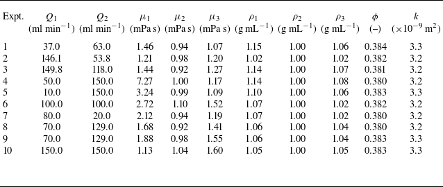
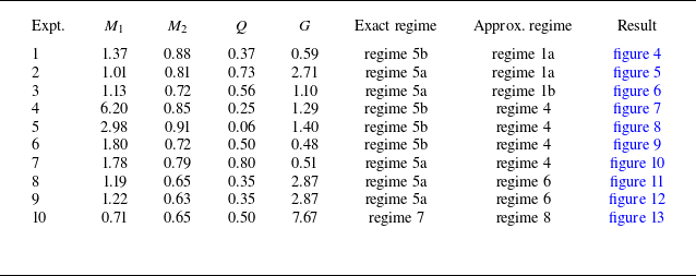
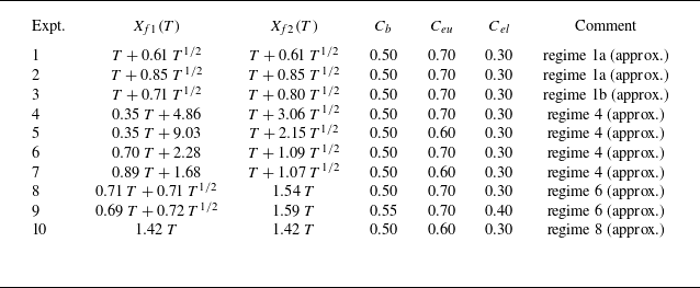
of the one-dimensional sharp-interface model (e.g. Zheng Reference Zheng2023; Yang & Zheng Reference Yang and Zheng2024). In addition, to provide a reproducibility check, the experimental parameters of experiment 9 are designed to be exactly the same as those of experiment 8, see also Appendix B for more detailed discussions. The values of the raw experimental parameters, as well as the dimensionless parameters, are summarised in tables 2 and 3 for all of the experiments performed in this work.
The experimental parameters for the interaction of two gravity currents in a confined porous layer. They were performed in a bead-packed Hele-Shaw cell that is
 $l=150$
cm in length,
 $h_0=10$
cm in depth and
 $w=3$
cm in width. The porosity
 $\phi$
is measured and the permeability
 $k$
is calculated based on
 $\phi$
and
 $r$
(radius of the beads). The area injection rates are estimated by
 $q_1 = Q_1/w$
and
 $q_2 = Q_2/w$
in the theoretical model.

Values of the dimensionless control parameters for the different experiments performed. Comments on the specific regime of each experiment are based on the one-dimensional sharp-interface model, depending on
 $\{M_1,M_2,Q,G\}$
. Experiment 9 is designed as a repeating one of experiment 8 to illustrate the reproducibility and is discussed in Appendix B as well.

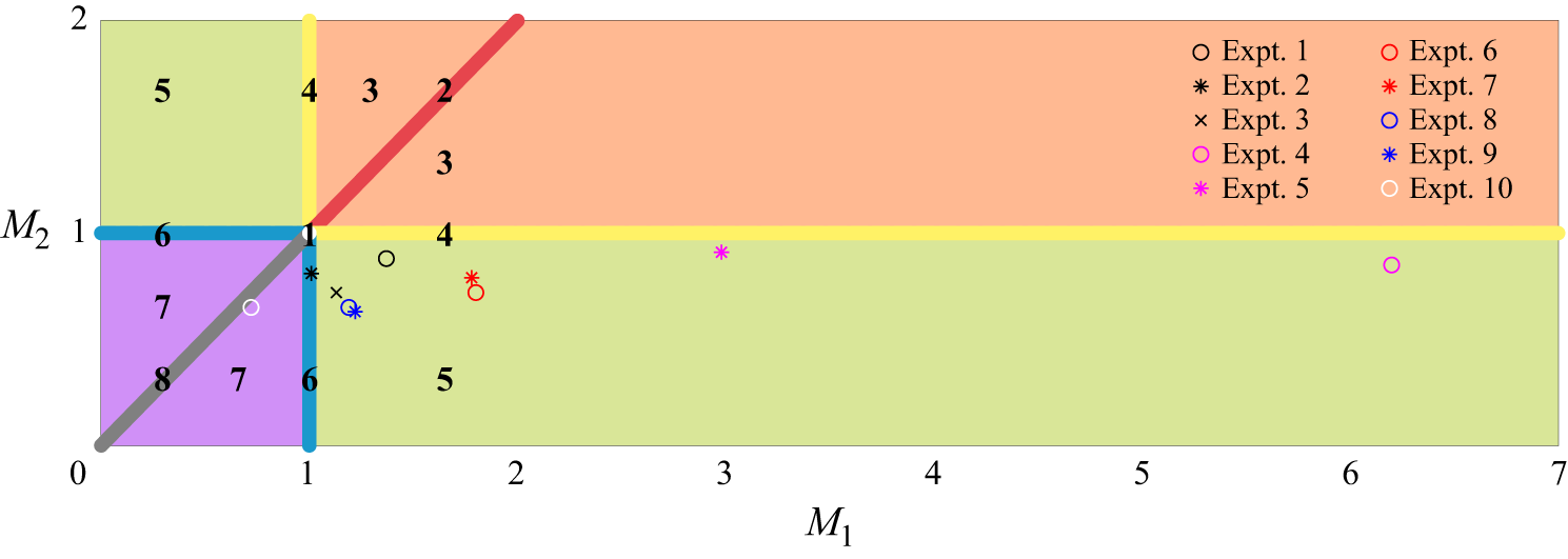
Based on the one-dimensional sharp-interface model of gravity current interaction (Yang & Zheng Reference Yang and Zheng2024), the performed laboratory experiments cover a total of three exact regimes, depending on the value of the four dimensionless parameters
 $\{M_1,M_2,Q,G\}$
. This is illustrated in the regime diagram in figure 3, and it is also illustrated that some of these experiments are located fairly close to the regime boundaries. In addition, when the influence of the viscosity ratio can be neglected, the experiments then cover as many as eight approximate regimes of gravity current interaction.
The regime diagram of gravity current interaction at late times based on the one-dimensional sharp-interface model (Yang & Zheng Reference Yang and Zheng2024), and the location of the ten performed experiments in this diagram. The regime diagram is symmetric about the diagonal line
 $M_1=M_2$
, so we only consider the region of
 $M_1 \geqslant M_2$
in the experimental design.

3. Experimental observations
In this section, we describe typical experimental observations on the profile shape evolution, along with the frontal dynamics, during the interaction of two viscous gravity currents. A comparison will then be attempted with the theoretical predictions, which allows us to obtain insights into both the agreement and disagreement between the theoretical and experimental results. For each experiment there exist both the corresponding exact regime and the appropriate approximate regime (if we are allowed to neglect the influence of the viscosity ratio between the fluids when they are fairly close to each other). Overall, the ten performed experiments cover three exact and eight approximate regimes, as summarised in figure 3 and table 3.
3.1. The profile shape evolution
We first describe major observations from these experiments on the time evolution of the profile shapes and concentration fields. Throughout the presentation, we provide a series of comparisons between the experimental observations and the theoretical predictions in both the exact regimes (e.g. in panel (a) of the figures 4–13) and the approximate regimes (e.g. in panel (b) of the figures 4–13). One would see some of the common features from the discussions next:
-
(i) For the experiments we performed, the time-dependent numerical solutions of the full partial differential system typically make reasonable predictions for the profile shape evolution and frontal dynamics in both the exact and approximate regimes. The numerical solutions in the exact regime typically work slightly better than those in the approximate regime, which is as expected.
-
(ii) This is not necessarily true for the self-similar solutions. In some of the exact regimes the self-similar solutions fail to work, while in the approximate regimes they actually work well. Our understanding is that this is predominantly related to the transition period for the self-similar solutions to fully develop: In some of the exact regimes the transition period is longer than the experimental period, but it is shorter than or comparable with the experimental period in the approximate regimes for the self-similar solutions to be observed.
-
(iii) For the experimental parameters considered in this work, we did not observe significant development of the fingering structures for the viscously unstable displacement processes (when the gravity current is less viscous than the ambient fluid). We argue this is because the buoyancy effects are sufficiently significant over the experimental time period for the injected fluids to predominantly develop as gravity currents.
-
(iv) Finally, in almost all of the experiments performed, there exists some degree of fluid mixing in the frontal regions of the currents and in the local regions where the three fluids meet. This is not considered in the one-dimensional sharp-interface models, and there exists more significant disagreement in these regions with the theoretical predictions. We do not comment on this feature any more in this section, but we do recognise this disagreement.
Comparison between the experimental observations (experiment 1) and the numerical/self-similar solutions: (a) the imposed experimental parameters are
 $\{M_1,M_2,Q,G\}=\{1.37,0.88,0.37,0.59\}$
in the model, corresponding exactly to regime 5b, and (b) the imposed experimental parameters are
 $\{M_1,M_2,Q,G\}=\{1.00,1.00,0.37,0.59\}$
in the model, neglecting the viscosity contrasts of the working fluids, which corresponds approximately to regime 1a. The green solid curves denote the time-dependent numerical solutions of the partial differential equations (PDEs) (A2a
,
b
) at dimensionless times
 $T=0.673\times \{1,2,3,4\}$
, while the white dashed curves denote the self-similar solutions at the same times.

Comparison between the experimental observations (experiment 2) and the numerical/self-similar solutions: (a) the imposed experimental parameters are
 $\{M_1,M_2,Q,G\}=\{1.01,0.81,0.73,2.71\}$
in the model, corresponding exactly to regime 5a, and (b) the imposed experimental parameters are
 $\{M_1,M_2,Q,G\}=\{1.00,1.00,0.73,2.71\}$
in the model, neglecting the viscosity contrasts of the working fluids, which corresponds approximately to regime 1a. The green solid curves denote the time-dependent numerical solutions of the PDEs (A2a
,
b
) at dimensionless times
 $T=15.8\times \{1,2,3,4\}$
, while the white dashed curves denote the self-similar solutions at the same times.

Comparison between the experimental observations (experiment 3) and the numerical/self-similar solutions: (a) the imposed experimental parameters are
 $\{M_1,M_2,Q,G\}=\{1.13,0.72,0.56,1.10\}$
in the model, corresponding exactly to regime 5a, and (b) the imposed experimental parameters are
 $\{M_1,M_2,Q,G\}=\{1.00,1.00,0.56,1.10\}$
in the model, neglecting the viscosity contrasts of the working fluids, which corresponds approximately to regime 1b. The green solid curves denote the time-dependent numerical solutions of the PDEs (A2a
,
b
) at dimensionless times
 $T=2.40\times \{1,2,3,4\}$
, while the white dashed curves denote the self-similar solutions at the same times.

3.1.1. Experiments 1–3: regime 5 (exact) vs regime 1 (approximate)
We first discuss experiments 1–3 in the same section here, because they correspond to the same exact and approximate regimes, and the take-home messages are similar when we impose a comparison between the experimental observations and the theoretical predictions. In all these experiments, fresh water and salt water are injected simultaneously from the top-left and bottom-left corners of the bead-packed Hele-Shaw cell, respectively, coloured with the blue and red dyes. The injected fluids then displace a third fluid of salt water with a different salt concentration, such that its density is in between the two injecting fluids. The two currents co-flow towards the downstream and displace the ambient fluid. The comparisons are shown in figures 4 to 6 for experiments 1–3, respectively.
They all correspond exactly to regime 5 (
 $M_1\gt 1\gt M_2$
) based on the measured values of the density, viscosity and injection rate of the fluids in use. The minor difference is that experiment 1 corresponds exactly to regime 5b since
 $Q \lt M_2(1-M_1)/(M_2-M_1)$
, while experiments 2 and 3 correspond exactly to regime 5a since
 $Q \geqslant M_2(1-M_1)/(M_2-M_1)$
. Meanwhile, they all correspond approximately to regime 1 (
 $M_1 = M_2 = 1$
), because the viscosity values of the three working fluids are almost the same. More strictly, experiments 1 and 2 correspond approximately to the symmetric regime 1a with
 $(1/Q-1/G) = 1$
, while experiment 3 corresponds approximately to the asymmetric regime 1b with
 $(1/Q-1/G) \ne 1$
.
In the (a) panels of figures 4–6, we impose the exact parameters in the numerical simulations based on the measured values:
 $\{M_1,M_2,Q,G\}=\{1.37,0.88,0.37,0.59\}$
for experiment 1 (regime 5b),
 $\{M_1,M_2,Q,G\}=\{1.01,0.81,0.73,2.71\}$
for experiment 2 (regime 5a) and
 $\{M_1,M_2,Q,G\}=\{1.13,0.72,0.56,1.10\}$
for experiment 3 (regime 5a). The time-dependent numerical solutions (the green solid curves) and the self-similar solutions (the white dashed curves) are then superimposed onto the experimental images for a comparison. In all three experiments, overall, we observe very good agreement between the time-dependent numerical solutions and the experimental profiles. However, there is almost no agreement between the self-similar solutions and the experimental observations, and to our understanding this is primarily due to the unfinished time transition for the self-similar solutions to fully develop in these experiments.
In the (b) panels of figures 4–6, we then neglect the viscosity difference between the three working fluids, and we impose the following approximate parameters in the numerical simulations:
 $\{M_1,M_2,Q,G\}=\{1.00,1.00,0.37,0.59\}$
for experiment 1 (regime 1a),
 $\{M_1,M_2,Q,G\}=\{1.00,1.00,0.73,2.71\}$
(regime 1a) for experiment 2 and
 $\{M_1,M_2,Q,G\}=\{1.00,1.00,0.56,1.10\}$
for experiment 3 (regime 1b). The simulation results are superimposed onto the experimental images as well, including the time-dependent numerical solutions (the green solid curves) and the self-similar solutions (the white dashed curves) at the same dimensionless times. Now we observe that the numerical and self-similar solutions both make reasonable predictions in all three experiments. We also observe good agreement between the time-dependent numerical solutions and the experimental profiles, and more interestingly, the self-similar solutions now make very reasonable predictions in these approximate regimes, which indicates that the transition is now finished (in the approximate regimes). We do note that the agreement is slightly worse in the (b) panels if we look particularly carefully at the profile shape between the upper and lower currents, compared with the numerical solutions in the exact regimes in the (a) panels. This, however, is as expected, because the influence of the viscosity contrasts has been considered appropriately in the exact regimes.
3.1.2. Experiments 4–7: regime 5 (exact) vs regime 4 (approximate)
We next show typical observations in experiments 4–7 in figures 7 and 10, respectively. They are discussed in the same section, because they all correspond to regime 5 (
 $M_1\gt 1\gt M_2$
) based on the exact parameters from measurements, while they all correspond approximately to regime 4 (
 $M_1\gt M_2=1$
) when the viscosity ratio is neglected between the upper current and the ambient fluid. There is also the subtle difference that experiments 4–6 correspond to regime 5b with
 $Q \lt M_2(1-M_1)/(M_2-M_1)$
, while experiment 7 corresponds to regime 5a with
 $Q \geqslant M_2(1-M_1)/(M_2-M_1)$
. In all these experiments, we see clearly that the lighter currents gradually move ahead of the heavier currents as time progresses and eventually wrap them up, a key feature of regime 4. The trend becomes clearer in experiments 4–6 within the time scale of the experiments, when we further reduce the relative injection rate of the heavier current in the experiments.
Comparison between the experimental observations (experiment 4) and the numerical/self-similar solutions: (a) the imposed experimental parameters are
 $\{M_1,M_2,Q,G\}=\{6.20,0.85,0.25,1.29\}$
in the model, corresponding exactly to regime 5b, and (b) the imposed experimental parameters are
 $\{M_1,M_2,Q,G\}=\{6.20,1.00,0.25,1.29\}$
in the model, neglecting the viscosity contrasts of the working fluids, which corresponds approximately to regime 4. The green solid curves denote the time-dependent numerical solutions of the PDEs (A2a
,
b
) at dimensionless times
 $T=11.1\times \{1,2,3,4\}$
, while the white dashed curves denote the self-similar solutions at the same times.

Comparison between the experimental observations (experiment 5) and the numerical/self-similar solutions: (a) the imposed experimental parameters are
 $\{M_1,M_2,Q,G\}=\{2.98,0.91,0.06,1.40\}$
in the model, corresponding exactly to regime 5b, and (b) the imposed experimental parameters are
 $\{M_1,M_2,Q,G\}=\{2.98,1.00,0.06,1.40\}$
in the model, neglecting the viscosity contrasts of the working fluids, which corresponds approximately to regime 4. The green solid curves denote the time-dependent numerical solutions of the PDEs (A2a
,
b
) at dimensionless times
 $T=6.23\times \{1,2,3,4\}$
, while the white dashed curves denote the self-similar solutions at the same times.

Comparison between the experimental observations (experiment 6) and the numerical/self-similar solutions: (a) the imposed experimental parameters are
 $\{M_1,M_2,Q,G\}=\{1.80,0.72,0.50,0.48\}$
in the model, corresponding exactly to regime 5b, and (b) the imposed experimental parameters are
 $\{M_1,M_2,Q,G\}=\{1.80,1.00,0.50,0.48\}$
in the model, neglecting the viscosity contrasts of the working fluids, which corresponds approximately to regime 4. The green solid curves denote the time-dependent numerical solutions of the PDEs (A2a
,
b
) at dimensionless times
 $T=5.01\times \{1,2,3,4\}$
, while the white dashed curves denote the self-similar solutions at the same times.

Comparison between the experimental observations (experiment 7) and the numerical/self-similar solutions: (a) the imposed experimental parameters are
 $\{M_1,M_2,Q,G\}=\{1.78,0.79,0.80,0.51\}$
in the model, corresponding exactly to regime 5a, and (b) the imposed experimental parameters are
 $\{M_1,M_2,Q,G\}=\{1.78,1.00,0.80,0.51\}$
in the model, neglecting the viscosity difference between the upper current and the ambient fluid, which corresponds approximately to regime 4. The green solid curves denote the time-dependent numerical solutions of the PDEs (A2a
,
b
) at dimensionless times
 $T=2.11\times \{1,2,3,4\}$
, while the white dashed curves denote the self-similar solutions at the same times.

In the (a) panels of figures 7 and 10, we impose the exact parameters in the numerical simulations:
 $\{M_1,M_2,Q,G\}=\{6.20,0.85,0.25,1.29\}$
for experiment 4 (regime 5b),
 $\{M_1,M_2,Q,G\}=\{2.98,0.91,0.06,1.40\}$
for experiment 5 (regime 5b),
 $\{M_1,M_2,Q,G\}=\{1.80,0.72,0.50,0.48\}$
for experiment 6 (regime 5b) and
 $\{M_1,M_2,Q,G\}=\{1.78,0.79,0.80,0.51\}$
for experiment 7 (regime 5a). The time-dependent numerical solutions (the green solid curves) and self-similar solutions (the white dashed curves) are then superimposed on the experimental images for a comparison. In all four experiments, we observe reasonable agreement between the time-dependent numerical solutions and the experimental observations. The self-similar solutions work well in experiments 6 and 7, but they fail in experiments 4 and 5 (and again this is likely due to the influence of unfinished time transition for the self-similar solutions to fully develop).
In the (b) panels of figures 7 and 10, in the numerical simulations the viscosity difference between the upper current and the ambient fluid has been neglected, and we impose the following approximate parameters:
 $\{M_1,M_2,Q,G\}=\{6.20,1.00,0.25,{}1.29\}$
for experiment 4,
 $\{M_1,M_2,Q,G\}=\{2.98,1.00,0.06,1.40\}$
for experiment 5,
 $\{M_1,M_2,Q,G\}=\{1.80,1.00,0.50,0.48\}$
for experiment 6 and
 $\{M_1,M_2,Q,G\}=\{1.78,1.00,0.80,0.51\}$
for experiment 7. They all correspond to regime 4, after making the approximation of
 $M_2 = 1$
. The simulation results are superimposed onto the experimental images as well at the same dimensionless times. Now we observe that the numerical and self-similar solutions both make reasonable predictions in all four experiments.
3.1.3. Experiments 8–9: regime 5a (exact) vs regime 6 (approximate)
We now discuss experiments 8–9 in the same section, because they both correspond exactly to regime 5a (
 $M_1\gt 1\gt M_2$
and
 $Q \geqslant M_2(1-M_1)/(M_2-M_1)$
), and approximately to regime 6 (
 $M_1=1\gt M_2$
) when the viscosity difference between the lower current and the ambient fluid is neglected (such that
 $M_1=1$
). Experiment 9 also provides a reproducibility check of experiment 8, as we discuss in Appendix B, in which the lower current is coloured with the green dye to be compared with the rest.
In the (a) panels of figures 11 and 12, we impose the exact parameters in the numerical simulations based on experimental measurements:
 $\{M_1,M_2,Q,G\}=\{1.19,0.65,0.35,2.87\}$
for experiment 8, and
 $\{M_1,M_2,Q,G\}=\{1.22,0.63,0.35,2.87\}$
for experiment 9. The time-dependent numerical solutions (the green solid curves) and self-similar solutions (the white dashed curves) of regime 5a are then superimposed onto the experimental images at representative times for a comparison. For both experiments, we have observed reasonable agreement between the numerical solutions, the self-similar solutions, and the experimental observations.
Comparison between the experimental observations (experiment 8) and numerical/self-similar solutions: (a) the imposed experimental parameters are
 $\{M_1,M_2,Q,G\}=\{1.19,0.65,0.35,2.87\}$
in the model, corresponding exactly to regime 5a, and (b) the imposed experimental parameters are
 $\{M_1,M_2,Q,G\}=\{1.00,0.65,0.35,2.87\}$
in the model, neglecting the viscosity contrasts of the working fluids, which corresponds approximately to regime 6. The green solid curves denote the time-dependent numerical solutions of the PDEs (A2a
,
b
) at dimensionless times
 $T=8.71\times \{1,2,3,4\}$
, while the white dashed curves denote the self-similar solutions at the same times.

Comparison between the experimental observations (experiment 9) and the numerical/self-similar solutions: (a) the imposed experimental parameters are
 $\{M_1,M_2,Q,G\}=\{1.22,0.63,0.35,2.87\}$
in the model, corresponding exactly to regime 5a, and (b) the imposed experimental parameters are
 $\{M_1,M_2,Q,G\}=\{1.00,0.63,0.35,2.87\}$
in the model, neglecting the viscosity contrasts of the working fluids, which corresponds approximately to regime 6. The green solid curves denote the time-dependent numerical solutions of the PDEs (A2a
,
b
) at dimensionless times
 $T=9.30\times \{1,2,3,4\}$
, while the white dashed curves denote the self-similar solutions at the same times.

In the (b) panels of figures 11 and 12, we further neglect the viscosity difference between the lower current and the ambient fluid (such that
 $M_1 = 1$
), and we impose the following approximate parameters in the numerical simulations:
 $\{M_1,M_2,Q,G\}=\{1.00,0.65,0.35,2.87\}$
for experiment 8, and
 $\{M_1,M_2,Q,G\}=\{1.00,0.63,0.35,2.87\}$
for experiment 9. The simulation results (of regime 6 now) are then superimposed onto the experimental images at the same dimensionless times. We also observe very good agreement between the theoretical predictions and the experimental observations.
3.1.4. Experiment 10: regime 7 (exact) vs regime 8 (approximate)
Finally, we show in figure 13 typical observations of the profile shape evolution of experiment 10. Note that in this experiment the ambient fluid is now coloured with the red dye, to be compared with other experiments. The displacement processes are viscously unfavourable during the injection of both the upper and lower currents. However, within the time and length scales of this experiment, we did not observe significant development of the viscous fingering structures. Instead, due to the influence of buoyancy, the upper and lower currents propagate along the horizontal boundaries, and the profile shapes are predominantly monotonic. We would argue that the reason for the suppressed development of the fingering structure is that the viscosity ratios are not large enough, and in the meantime the buoyancy effects are sufficiently significant for both the upper and lower injecting fluids to develop as gravity currents.
Comparison between the experimental observations (experiment 10) and the numerical/self-similar solutions: (a) the imposed experimental parameters are
 $\{M_1,M_2,Q,G\}=\{0.71,0.65,0.50,7.67\}$
in the model, corresponding exactly to regime 7, and (b) the imposed experimental parameters are
 $\{M_1,M_2,Q,G\}=\{0.65,0.65,0.50,7.67\}$
in the model, neglecting the viscosity contrasts of the working fluids, which corresponds approximately to regime 8. The green solid curves denote the time-dependent numerical solutions of the PDEs (A2a
,
b
) at dimensionless times
 $T=25.5\times \{1,2,3,4\}$
, while the white dashed curves denote the self-similar solutions at the same times.

The dimensionless parameters are
 $\{M_1,M_2,Q,G\}=\{0.71,0.65,0.50,7.67\}$
based on the measured values of the density, viscosity and injection rates, which corresponds to regime 7 (
 $1\gt M_1\gt M_2$
). The theoretical predictions are then superimposed onto the experimental images in figure 13(a), including the time-dependent numerical solutions (the green solid curves) and the self-similar solutions (the white dashed curves) at dimensionless times
 $T=25.5\times \{1,2,3,4\}$
. We have observed that both the numerical and self-similar solutions (in regime 7) make reasonable predictions for this experiment. Also, the numerical solutions and self-similar solutions are fairly close to each other, which suggests the time transition is almost finished for the self-similar solutions to fully develop. There is also some over-prediction for the profile shape of the lower current, which is most likely due to fluid mixing and two-dimensional flow effects.
Because
 $M_1$
and
 $M_2$
are fairly close to each other, this experiment also corresponds to regime 8 (
 $1\gt M_1=M_2$
), approximately, if we neglect this difference. Similarly, we then include the theoretical predictions of the profile shapes with
 $\{M_1,M_2,Q,G\}=\{0.65,0.65,0.50,7.67\}$
in figure 13(b), including both the time-dependent numerical solutions (the green solid curves) and the self-similar solutions (the white dashed curves) and at the same dimensionless times. The result is very similar to what we observed in figure 13(a): the numerical and self-similar solutions (in regime 8 now) both make very reasonable predictions for this experiment.
More details on figure 14:
 $\{X_{\!f1}, X_{\!f2}\}$
represent the self-similar solutions in the exact regimes base on experimentally measured parameters;
 $\{C_b,C_{\textit{eu}},C_{\textit{el}}\}$
are the threshold values of the signal intensity dealing with the frontal location of the experimental pictures, employing the Matlab subroutine ‘contour3’;
 $C_b$
represents the base-case threshold value for the frontal location while
 $C_{\textit{eu}}$
and
 $C_{\textit{el}}$
represent the threshold values that correspond to the upper and lower error bars.

3.2. The frontal dynamics
We can also track the location of the propagating fronts in these experiments, along with a comparison with theoretical predictions of the sharp-interface model of viscous gravity current interaction, as shown in figure 14 (based on the three exact regimes) and figure 15 (based on the eight approximate regimes). In particular, we now include the time-dependent experimental data for the location of both the upper current (as denoted by
 $X_{\!f2}(T)$
) and the lower current (as denoted by
 $X_{\!f1}(T)$
) at representative times. Note that the dimensionless frontal location is defined as
 $X_f \equiv x_f/x_c$
, which is plotted against the dimensionless time
 $T \equiv t/t_c$
, and they are appropriately rescaled based on the following characteristic scales
 \begin{align} x_c=\frac {\Delta \rho _1 gk h_0^2 }{\mu _1 q},\quad \mathrm{and} \quad t_c=\frac {\Delta \rho _1 g k h_0^3 \phi }{\mu _1 q^2}, \end{align}
where
 $\Delta \rho _1 = \rho _1 - \rho _3$
and
 $q = q_1+q_2$
. These scales arise due to the competition between buoyancy and injection forces and are chosen such that the prefactors become one in the dimensionless governing equations, see Appendix A.
The dimensionless frontal locations in experiment 1 to experiment 10: the red symbols represent the dimensionless locations of the lower front
 $X_{\!f1}(T)$
, while the blue symbols represent the dimensionless locations of the upper front
 $X_{\!f2}(T)$
. As a comparison, the self-similar solutions of PDEs (A2a
,
b
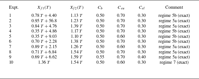
) are included as the dashed curves, while the time-dependent numerical solutions are included as the solid curves. Here, we use the experimentally measured parameters in the model, corresponding to the exact flow regimes. More details are provided in table 4 on the self-similar solutions obtained for different experiments and the threshold values imposed to obtain the frontal location and error bars from the experimental images.

The dimensionless frontal locations of experiment 1 to experiment 10: the red symbols represent the dimensionless locations of the lower front
 $X_{\!f1}(T)$
, while the blue symbols represent the dimensionless locations of the upper front
 $X_{\!f2}(T)$
. As a comparison, the self-similar solutions of PDEs (A2a
,
b
) are included as the dashed curves, while the time-dependent numerical solutions are included as the solid curves. Here, we neglect the viscosity contrasts when appropriate in the model, corresponding to the approximate flow regimes. More details are provided in table 5 on the self-similar solutions obtained for different experiments and the threshold values imposed to obtain the frontal location and error bars from the experimental images.

Due to fluid mixing, the frontal locations are detected based on the signal intensity of the experimental pictures, employing Matlab subroutine ‘contour3’ to provide the equal-intensity contours. It requires input of a threshold intensity value
 $C$
for the signal intensity. In this work, we impose
 $C_b$
for the base-case estimate of the frontal location, while we impose
 $C_{\textit{eu}}$
and
 $C_{\textit{el}}$
for the upper and lower error bars. Typical values we found to provide reasonable estimates are
 $\{C_b,C_{\textit{eu}},C_{\textit{el}}\} = \{0.5,0.7,0.3\}$
, which are imposed for both the upper and lower currents in the same experiment. The specific values of
 $\{C_b,C_{\textit{eu}},C_{\textit{el}}\}$
imposed in experiment 1 to experiment 10 are provided in table 4 (for the exact regimes) and table 5 (for the approximate regimes). Experiment 9 provides a reproducibility check of experiment 8 and is discussed in Appendix B. This procedure is similar to the previous treatment of mildly miscible displacement in porous media at small Reynolds numbers (e.g. Sahu & Neufeld Reference Sahu and Neufeld2020; Rathore, Zheng & Sahu Reference Rathore, Zheng and Sahu2025). This procedure is also similar to the previous treatment of turbulent gravity currents regarding the influence of fluid mixing and turbulent entrainment at large Reynolds numbers (e.g. Hacker, Linden & Dalziel Reference Hacker, Linden and Dalziel1996; Fragoso, Patterson & Wettlaufer Reference Fragoso, Patterson and Wettlaufer2013). More details on how we use ‘contour3’ are provided in Appendix C, with an example calculation on how to detect the equal-intensity contours and frontal locations from a representative experimental picture, along with the estimates for the error bars.
More details on figure 15:
 $\{X_{\!f1}, X_{\!f2}\}$
represent the self-similar solutions of the approximate regimes, neglecting the viscosity difference of the fluids when appropriate;
 $\{C_b,C_{\textit{eu}},C_{\textit{el}}\}$
are the threshold values of the signal intensity dealing with the frontal location of the experimental pictures, employing the Matlab subroutine ‘contour3’;
 $C_b$
represents the base-case threshold value for the frontal location while
 $C_{\textit{eu}}$
and
 $C_{\textit{el}}$
represent the threshold values that correspond to the upper and lower error bars.

With the experimental data available for the frontal dynamics, we are then able to make a suitable comparison with the prediction of the one-dimensional theoretical model of the sharp-interface type (e.g. Zheng Reference Zheng2023; Yang & Zheng Reference Yang and Zheng2024). The predictions are affected by the four dimensionless control parameters
 $\{M_1, M_2, Q, G\}$
, as measured in the experiments. We first include the time-dependent numerical solutions of the governing advective–diffusive PDEs (i.e. (A2a
,
b
) in Appendix A) as the solid curves. We observe very reasonable agreement between the numerical solutions and the experimental results, knowing that there is always the influence of fluid mixing, two-dimensional flow and local heterogeneity near the horizontal boundaries of the packed-bed system. We then include the self-similar solutions as the dashed curves in the same figure, which are expected to work at intermediate times. The predicted self-similar frontal dynamics is summarised in table 4 (for the three exact regimes) and table 5 (for the eight approximate regimes). We note that there are situations when the self-similar solutions do not make good predictions any more, in particular in the exact regimes, and to our understanding this is likely due to the influence of unfinished time transition. Overall, the degree of agreement/disagreement is consistent with our previous discussions on the profile shape evolution.
3.3. The time transition
While the time-dependent numerical solutions always make reasonable predictions for the profile shape evolution in the performed laboratory experiments, we have also observed that the self-similar solutions do not as always make as reasonable predictions. We have attributed this disagreement to the unfinished time transition towards the self-similar asymptotes. In our previous study (Yang & Zheng Reference Yang and Zheng2024), we have shown that the transition time is typically up to
 $\mathcal{O}(10^2)$
or
 $\mathcal{O}(10^3)$
in most of the simulations. In contrast, for the performed experiments of the present work the finishing time is typically of
 $\mathcal{O}(10)$
, which indicates that the time transition may not have finished yet by the end of the experiments.
To further support this argument, we take experiment 1 as an example, and we perform additional numerical simulations to show the time transition. To understand why the self-similar solutions of over-riding flows fail to make reasonable predictions in figure 4(a), we now impose
 $\{M_1,M_2,Q,G\}=\{1.37,0.88,0.37,0.59\}$
for its exact regime 5b, and run the simulation for a longer period of time (until
 $T = 500$
), compared with the experimental time (until
 $T \approx 2.7$
). The results are shown in figure 16, when we include both the time-dependent numerical solutions (the solid curves) and the self-similar solutions (the dashed curves) for the profile shape evolution. We now observe very reasonable predictions of the self-similar solutions of over-riding flows of regime 5b. These calculations demonstrate that the unfinished time transition is indeed the reason for the disagreement observed in figure 4(a), when the self-similar solutions fail to make reasonable predictions.
The time transition towards the self-similar solution for experiment 1 in its exact regime 5b of over-riding flow, imposing
 $\{M_1,M_2,Q,G\}=\{1.37,0.88,0.37,0.59\}$
. We show a comparison of the predicted profile shapes between the time-dependent numerical solutions (the solid curves) and the self-similar solutions (the dashed curves). Here, we run the simulation for a longer period of time (until
 $T = 500$
) than the experimental time (until
 $T \approx 2.7$
). We now observe reasonable predictions of the self-similar solutions.

In fact, based on the form of the self-similar solutions, we can obtain more analytical insights regarding the time transition in regime 1a (of co-flowing currents) and regime 5b (of over-riding flow).
-
(i) We first consider regime 1a of co-flowing currents. For the late-time self-similar solution to apply, it is required that the point where the three fluids meet, as denoted by
 $X = X_*(T)$
, should always exist, i.e. we must have
$X_* \gt 0$
. Based on the self-similar solution in regime 1a, we obtain that
$X_* = T - (QT)^{1/2} \gt 0$
, which leads to an estimate of
$T \gt 0.37$
for experiment 1. That said, in experiment 1, which ends at
$T \approx 2.7$
, there is sufficient time for the transition to finish in the approx. regime 1a. And, indeed, we observe very reasonable predictions for the profile shape evolution based on the self-similar solutions in figure 4(b).
-
(ii) We then consider regime 5b of over-riding flow. For the self-similar solution to apply, it is required that the trailing front
$X_{\!f3}(T)$
of the upper current must remain ahead of the leading front
$X_{\!f1}(T)$
of the lower currents along the bottom boundary, i.e. we must have
$X_{\!f3}(T) \gt X_{\!f1}(T)$
. Based on the self-similar solution of over-riding flow in regime 5b, we obtain that
$X_{\!f3}(T) = M_2T$
and
$X_{\!f1}(T) = C_1T + \theta _{\!f1}$
, where(3.2)Substituting in the experimental parameters, we obtain
\begin{equation} C_1 = M_1^{-1}M_2 + (1-M_1^{-1}M_2)Q,\,\,\, \theta _{\!f1} = \frac {(1+G^{-1})[M_1^{-1}M_2(1-Q)+C_1]}{2G^{-1}C_1^2(1-M_1^{-1}M_2)}. \end{equation}
$C_1 \approx 0.77$
,
$\theta _{\!f1} \approx 4.40$
and then an estimate of
$T \gt 40$
for the transition time. We then see that in experiment 1, which ends at
$T \approx 2.7$
, there is not enough time for the time transition to finish in the exact regime 5b to develop the self-similar solution of over-riding flow. Indeed, we observe that the over-riding flow pattern in regime 5b has not yet developed in experiment 1 in figure 4(a).


3.4. Potential implications
Before we close this paper, we briefly address the potential implications of the model and its solutions by investigating the sweep efficiency in regime 7, when the invading fluids are both less viscous than the ambient fluid and more specifically the situation of
 $\mu _1\lt \mu _2\lt \mu _3$
(i.e.
 $1 \gt M_1 \gt M_2$
). Such a situation mimics the displacement process of co-flooding CO
 $_2$
and water to displace oil for the co-profits of geological CO
 $_2$
sequestration and enhanced oil recovery.
The sweep efficiency
 $\varPsi (t)$
provides one of the most important quantitative measurements for a flooding technology in petroleum engineering, and by definition it is given by
 \begin{equation} \varPsi (t) \equiv \frac {V_1(t)+V_2(t)}{V_1(t)+V_2(t)+V_3(t)} = \frac {q_1+q_2}{h_0l_0}t, \end{equation}
in a two-dimensional configuration, where
 $V_1(t)$
,
 $V_2(t)$
and
 $V_3(t)$
represent the total volumes of fluids 1, 2 and 3 within the rectangular domain, respectively,
 $h_0$
and
 $l_0$
are the thickness and length of the domain and
 $q_1$
and
 $q_2$
are the area injection rates. In practice,
 $l_0$
could also be the distance between the injection and production wells. Of particular interest is the sweep efficiency
 $\varPsi _b \equiv \varPsi (T_b)$
at the (dimensionless) breakthrough time
 $T_b$
, defined as when the leading front of the two currents reaches the farther end of the domain (
 $X=L$
).
Here we focus on regime 7 for the application of co-flooding CO
 $_2$
and water in an oil field, and based on the self-similar solution of this regime, which predicts that the leading front of the two currents locates at
 $X_{\!f}(T) = T/M_2$
, we further obtain that
 \begin{equation} \varPsi _b = M_2, \end{equation}
at the breakthrough time. The result depends only on the viscosity ratio
 $M_2 \equiv \mu _2/\mu _3$
, and is independent on the dimensionless domain length
 $L$
. We must also note that the calculations here have neglected the potential two-dimensional fingering effects due to unfavourable viscosity contrasts, which are assumed to have been suppressed by the buoyancy effects. We also note that experiment 10 lies in this regime, and based on the experimental measurement of the viscosity of the working fluids, we obtain that
 $M_2 = 0.65$
for this experiment. We process further data analysis based on the experimental picture when the leading front reaches the end of the domain (at
 $t \approx 240$
s in figure 13), and we found that
 $\varPsi _b = 0.58$
(or
 $\varPsi _b \in (0.51, 0.63)$
), which is consistent with (reasonably close to) the theoretical result (3.4). Here, the threshold values
 $\{C_b,C_{\textit{eu}},C_{\textit{el}}\}$
to detect the contour shape of the currents are chosen to be the same as those when we detect the frontal dynamics in table 4.
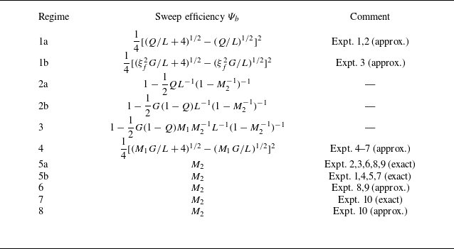
Finally, for completeness of the analysis and regardless of the specific fluids in use in different applications, we provide analytical solutions for the sweep efficiency
 $\varPsi _b$
at the breakthrough time in the other ten asymptotic regimes of gravity current interaction. In fact, we can obtain that
 $\varPsi _b = T_b/L$
based on global mass conservation, since the sum of the dimensionless area injection rates of the two currents is one. Assuming that there is enough time for the flow to develop into a self-similar fashion, we further obtain the value of
 $T_b$
based on the self-similar solutions for the location of the faster front in different self-similar regimes of gravity current interaction. The results are summarised in table 6. As it turns out that, in regimes 5–8, the solutions of
 $\varPsi _b$
are independent on the length of the domain
 $L$
. This is because at leading order the faster front advances at a constant speed at intermediate times. In contrast, in regimes 1–4, the faster front advances nonlinearly as a key feature of equal-viscosity displacement and, correspondingly, the solutions for
 $\varPsi _b$
depend on the domain length
 $L$
. To summarise, it is seen that
 $\varPsi _b$
could possibly be under the influence of the four dimensionless parameters
 $\{M_1,M_2,G,Q\}$
, as well as the dimensionless domain length
 $L$
. One can justify accordingly which solution to use appropriately in table 6, depending on the specific regime of gravity current interaction.
More details on the sweep efficiency
 $\varPsi _b$
at the breakthrough time
 $T_b$
in different interaction reigmes of heavier and lighter currents in a confined aquifer. For regime 1b,
 $\xi _f^2 = a_1^2/b_1^2$
, and
 $a_1(G,Q)$
and
 $b_1(G,Q)$
are two constants that depend on
 $(G,Q)$
, as given by equations (D3a,c) in the appendix of Yang & Zheng (Reference Yang and Zheng2024).

4. Summary and final remarks
We have investigated in this paper the dynamic interaction of two viscous gravity currents within a porous layer of finite depth. Compared with our previous studies (e.g. Zheng Reference Zheng2023; Yang & Zheng Reference Yang and Zheng2024) focusing primarily on theoretical and asymptotic analyses, we now investigate the problem using a series of laboratory experiments in a vertically placed bead-packed Hele-Shaw cell. We have included a total of ten laboratory experiments, which allows us to visualise the time evolution of the profile shape, frontal location and concentration fields during the injection and interaction of a upper lighter current and another lower heavier current.
By varying the density, viscosity and injection rate of the working fluids, these experiments were designed to cover three exact and eight approximate regimes (by neglect the influence of viscosity ratio when it is close to one) of viscous current interaction, as determined by the value of the four dimensionless parameters
 $\{M_1, M_2, G, Q\}$
based on the one-dimensional sharp-interface model (see also table 7). We have observed that the time-dependent numerical solutions typically make reasonably good predictions in both the exact and approximate regimes, and in the exact regimes they make slightly better predictions for the region where the upper and lower currents meet (by considering the influence of the viscosity ratio). In contrast, the self-similar solutions in some of the exact regimes do not appear to work, and this is due to the unfinished time transition for them to fully develop. Interestingly, the self-similar solutions in the approximate regimes typically work well.
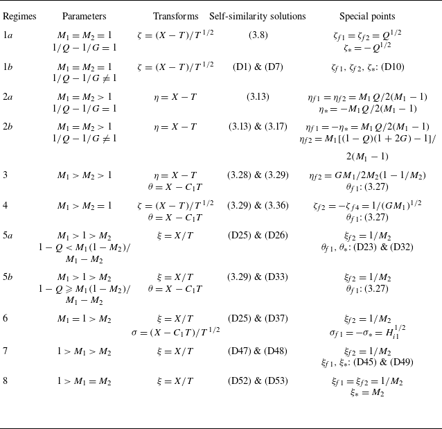
Parameters, transforms, solutions and special points in the different regimes of two current interaction, as modified from table 2 of Yang & Zheng (Reference Yang and Zheng2024). Note that, here,
 $M_1$
is their
 $M_2$
,
 $M_2$
is their
 $M_2/M_3$
and the propagation speed is
 $C_1 = M_2/M_1+(1-M_2/M_1)Q$
.

Overall, the performed experiments provide useful validations of the one-dimensional sharp-interface model, which has reasonably captured the time evolution of the profile shape and frontal location of the currents for the experimental parameters we considered. These exists some minor disagreement predominantly in the frontal region of the currents, which is likely due to the influence of fluid mixing and two-dimensional flow effects. The experimental observations made have further advanced our fundamental understandings on the propagation, displacement and interaction of multiple fluid layers within a confined porous layer, which are relevant in geophysical, environmental and industrial applications. This is particularly true, knowing that the dynamics is very rich with up to eleven distinct regimes of current interaction and some of the asymptotic solutions cannot be obtained simply by combining appropriately the four solution branches of single current injection.
Future work is also motivated to further explore the intermediate regime between gravity current and viscous fingering in the context of gravity current interaction. It would be of use to explore the parameter range when the viscous fingering instability significantly develops, perhaps with the help of two-dimensional numerical simulations in the miscible regime (e.g. Ruith & Meiburg Reference Ruith and Meiburg2000; Jha, Cueto-Felgueroso & Juanes Reference Jha, Cueto-Felgueroso and Juanes2011; Nijjer, Duncan & Neufeld Reference Nijjer, Duncan and Neufeld2018). This must also be treated carefully regarding the dispersion effects in the pore networks (e.g. Taylor Reference Taylor1953; Aris Reference Aris1956). For single fluid injection, recent simulations by Nijjer et al. (Reference Nijjer, Duncan and Neufeld2018) indicate that the fingering instabilities could be suppressed under dispersion effects at intermediate times, while Hinton & Jyoti (Reference Hinton and Jyoti2022) show that buoyancy segregation could also suppress the fingering instability for radial currents. From the application point of view, it may also be of use to explore the vertically averaged properties and their parametric dependence for quick insights into practical contexts.
Finally, potential implications of the model and solutions are also briefly discussed by investigating the sweep efficiency in regime 7, which corresponds to co-flooding CO
 $_2$
and water to displace oil for the co-profits of geological CO
 $_2$
sequestration and enhanced oil recovery. In this case, there exists an analytical solution of
 $\varPsi _b = M_2 \equiv \mu _2/\mu _3$
at the breakthrough time
 $t = t_b$
, which is reasonably close to the experimental value of experiment 10 (figure 13). We must note that in the model we have neglected the influence of fluid mixing (in the miscible regime) or interfacial tension (in the immiscible regime), as well as the two-dimensional development of the interfacial instabilities, which must be treated carefully in practical contexts.
Funding
We acknowledge partial support from an Eastern Scholar Distinguished Professorship (No. TP2020009) and NSFC (No. 12272235).
Declaration of interests
The authors report no conflict of interest.
Appendix A. Theoretical model
For clarity of the presentation, we include the dimensionless governing equations for the dynamic interaction of the two viscous gravity currents in a confined porous layer of finite depth, along with the appropriate initial and boundary conditions. This is to illustrate where the dimensionless parameters (
 $M_1$
,
 $M_2$
,
 $G$
and
 $Q$
) appear in the governing system, and how they may affect the dynamics of gravity current interaction. This could be of use along with the discussions of the experimental results.
In particular, the coupled advective-diffusive equations for the interface-shape evolution are given by
 \begin{equation} \frac {\partial H_1}{\partial T} + \frac {\partial Q_1}{\partial X}= 0,\,\,\,\frac {\partial \hat H_2}{\partial T} + \frac {\partial Q_2}{\partial X}= 0, \end{equation}
where the profile shape of the two currents are denoted by
 $H_1(X,T)$
and
 $\hat H_2(X,T)$
, measured from either the top or the bottom boundary, and the fluxes
 $Q_1(X,T)$
and
 $Q_2(X,T)$
are defined as
 \begin{align} Q_1(X,T) \equiv \frac {M_2H_1-[M_2(1-H_1-\hat {H}_2)+\hat {H}_2]M_1H_1\dfrac {\partial H_1}{\partial X}+GM_1H_1\hat {H}_2\dfrac {\partial \hat {H}_2}{\partial X} }{M_2H_1+M_1M_2(1-H_1-\hat {H}_2)+M_1\hat {H}_2}, \end{align}
 \begin{align} Q_2(X,T) \equiv \frac {M_1\hat {H}_2-[M_1(1-H_1-\hat {H}_2)+H_1]GM_1\hat {H}_2\dfrac {\partial \hat {H}_2}{\partial X}+ M_1H_1\hat {H}_2\dfrac {\partial H_1}{\partial X}}{M_2H_1+M_1M_2(1-H_1-\hat {H}_2)+M_1\hat {H}_2}, \end{align}
including an injection-driven component and two buoyancy-driven components that are related to the slope of the interfaces.
The coupled evolution equations (A2a , b ) are to be solved subject to appropriate dimensionless initial conditions
 \begin{align} H_1(X,0)=0,\,\,\, \hat {H}_2(X,0)=0, \end{align}
and boundary conditions
 \begin{align} H_1(X_{\!f1}(T),T) &= 0,\\[-12pt]\nonumber \end{align}
 \begin{align} \hat {H}_2(X_{\!f2}(T),T) & = 0,\\[-12pt]\nonumber \end{align}
 \begin{align} Q_1(0,T) & = Q,\\[-12pt]\nonumber \end{align}
 \begin{align} Q_2(0,T) & = 1-Q,\qquad \quad \end{align}
in the form of frontal and flux conditions imposed at
 $X=X_{fi}$
and
 $X=0$
, respectively.
It is ready to see that four dimensionless parameters
 $M_1$
,
 $M_2$
,
 $G$
and
 $Q$
have been recognised, and their definition and physical meaning are described in table 1. For more details on the derivations of the self-similar solutions at intermediate times (e.g. Barenblatt Reference Barenblatt1979), along with the numerical scheme to solve for the profile shapes
 $H_1(X,T)$
and
 $\hat H_2(X,T)$
, one can refer to our previous study (e.g. Yang & Zheng Reference Yang and Zheng2024), and we do not repeat the derivations. For clarify of presentation, we include a table 7 on the late-time self-similar solutions of gravity current interaction here. This is exactly table 2 of Yang & Zheng (Reference Yang and Zheng2024), but we note that the notations are slightly different from Yang & Zheng (Reference Yang and Zheng2024): in the present work
 $M_1$
is their
 $M_2$
,
 $M_2$
is their
 $M_2/M_3$
and then (A1) becomes exactly their (2.16).
Appendix B. Reproducibility check
To check the reproducibility of the experiments, we now perform a repeating experiment (experiment 9), using exactly the same parameters of experiment 8 that corresponds to regime 6. For these experiments, glycerine–water mixtures were used as the ambient fluid and the heavier injecting fluid, while fresh water was used as the lighter injecting fluid. The measured injection rates are
 $Q_1=70.0$
ml min−1 and
 $Q_2=129.0$
ml min−1, the viscosity of the working fluids are
 $\mu _1 = 1.88$
mPa
 $\,$
s,
 $\mu _2 = 0.98$
mPa
 $\,$
s and
 $\mu _3 = 1.55$
mPa
 $\,$
s, and the density of the working fluids are
 $\rho _1 = 1.06$
mPa
 $\,$
s,
 $\rho _2 = 1.00$
mPa
 $\,$
s and
 $\rho _3 = 1.04$
mPa
 $\,$
s, respectively. Meanwhile, the porosity of the bead-packed Hele-Shaw system is measured as
 $\phi =0.383$
, which leads to a permeability of
 $k=3.3\times 10^{-9}$
m
 $^2$
based on the Kozeny–Carman formula. These values are all reasonably close to if not exactly identical to the reported values of experiment 8, as summarised in table 2. In particular, for the working fluids, the density and injection rate values are exactly the same, while there is slight difference for the measured viscosity values (which is likely due to small variation of the room temperature and measurement error). The measured porosity and permeability values of the packed bed are also reasonably close.
We then compare the observations at representative times of these two experiments 8 and 9. In particular, the recorded pictures at
 $t =75 \times \{1,2,3,4\}$
s are included in figure 17(a,b) for these two runs, respectively. It is seen that the profile shapes are almost identical at the corresponding times in these two experiments, which provides a validation of the reproducibility of the experiments. Comparison between typical observations of experiment 9 and the theoretically predicted profile shapes is shown in figure 13.
(a) Representative experimental pictures at
 $t =75 \times \{1,2,3,4\}$
s in experiment 8, and (b) representative experimental pictures at
 $t =75 \times \{1,2,3,4\}$
s in experiment 9, which is designed to provide a reproducibility check of experiment 8, as an example.

Appendix C. Detecting the frontal location
Due to the influence of fluid mixing, we now employ Matlab subroutine ‘contour3’ to detect the time-dependent frontal locations of the experimental pictures, which requires input of a threshold value of the signal intensity to plot an equal-intensity contour. We also use the subroutine ‘imgaussfilt’ to reduce the oscillations of frequency higher than
 $f = 60$
(per pixel) in all of the experiments. The frontal location is defined as when the signal intensity first drops to a threshold value (e.g.
 $C_b = 0.50$
, the normalised Red/Green/Blue intensity value by its maximum in the pictures) along either the top/bottom boundary, i.e. when the equal-intensity contour intercepts the horizontal boundaries. An error estimate is also made possible by imposing other threshold values such as
 $C_{\textit{eu}} = 0.70$
and
 $C_{\textit{el}} = 0.30$
for the upper and lower estimates of the frontal location, respectively. To be self-consistent, for the same experiments, we use the same threshold values
 $\{C_b,C_{\textit{eu}},C_{\textit{el}}\}$
to deal with the frontal location of both the upper and lower currents for all times. The error bars employed here are defined based solely on the degree of fluid mixing, and do not reflect any measurement uncertainties of the density, viscosity, and injection rate of the working fluids, as well as the permeability and porosity of the packed porous bed.
An example calculation is illustrated in figure 18 on how we obtain the frontal locations based on a representative experimental picture at a specific time
 $t = 8$
min of experiment 1. The upper current is coloured with blue dye, while the lower current is coloured with red dye. Accordingly, we use the B-channel signals to deal with the upper current in the data analysis, while we use the R-channel signals for the lower current. Specifically, for the upper current, we deal with the normalised signals in the R-channel, and it turns out that the blue region can be distinguished from the red and white regions, which leads to figure 18(b). For the lower current, we deal with the normalised signals in the B-channel, but note that the red region can only be distinguished from the white region but not the blue region (because the blue region is too dark in the experiment). To obtain sensible signals only to the red region, the normalised values in the B channel are then subtracted by that of the R-channel, and then plus one. We found that this treatment works well and leads to figure 18(c). Furthermore, for both currents, we have included several different equal-intensity contours corresponding to different threshold values of the signal intensity. One is hence able to obtain insights into how it works, e.g. by imposing a base value (
 $C_b = 0.50$
) to define the frontal location, a greater value (
 $C_{\textit{eu}} = 0.70$
) to define the corresponding upper error bar, and a smaller value
 $C_{\textit{el}} = 0.30$
to define the lower error bar.
Detection of the frontal locations from a representative experimental picture using Matlab subroutine “contour3” which requires the input of a threshold value for the signal intensity: (a) raw experimental picture at time
 $t = 8.0$
min in experiment 1, (b) the contour plot of the upper current with different threshold values and (c) the contour plot of the lower current with different threshold values. The
 $x$
and
 $y$
labels are the pixel numbers in all three panels. In this experiment, the frontal location is defined as when the signal intensity reduces to
 $C_b = 0.50$
along the top/bottom boundary, and the upper and lower error bars are obtained when the intensity reduces to
 $C_{\textit{eu}} = 0.70$
and
 $C_{\textit{el}} = 0.30$
, respectively.

The frontal location is typically defined as the point where the specific equal-intensity contour intercepts with the upper/lower horizontal boundary. For sufficiently small threshold values of the signal intensity, we sometimes observe non-monotonic equal-intensity contours, and in this case the frontal location is defined as the point that is the farthest away from the origin, rather than the intercept of the equal-intensity contour with the horizontal boundaries. Such an issue is likely due to the fact that the injection points are slightly above/below the impermeable horizontal boundaries rather than perfectly aligning with them. When we defect the lower error bars, we have tried to impose a sufficiently large
 $C_{\textit{el}}$
to avoid this issue, such that the definitions are more clean and self-consistent. The values of
 $\{C_b,C_{\textit{eu}},C_{\textit{el}}\}$
we used are provided in tables 4 and 5 for all data points included in this paper. Imposing other reasonable values of
 $\{C_b,C_{\textit{eu}},C_{\textit{el}}\}$
is also allowed, which, however, would not change the major take-home message.