Measure and Data

I adopt Fryer and Levitt’s (2004) summary measure, termed Black Name Index (BNI), to capture the racial content of names. This index indicates how likely a name is to be held by blacks compared with whites and is computed as:

(1) $$BN{I_{name,j,g}} = 100 \cdot {{{{Black{s_{name,j,g}}} \over {Black{s_{j,g}}}}} \over {{{Black{s_{name,j,g}}} \over {Black{s_{j,g}}}} + {{White{s_{name,j,g}}} \over {White{s_{j,g}}}}}},$$

where the subscripts name, j, and g denote a given first name, birth year cohort, and gender, respectively. The components Blacks and Whites refer to the number of non-Hispanic native-born blacks and whites in each name-cohort-gender or cohort-gender combination. By construction, BNI ranges from 0 to 100. Names with a BNI of 0 are only held by whites, while names that have a BNI of 100 can only be found among blacks. Between these extremes, names that are equally likely to be used by both races have a BNI of 50.

To calculate BNI in a historical setting, I draw on the complete census records from 1870 to 1940 provided by IPUMS (Ruggles et al. Reference Ruggles, Sarah Flood, Josiah Grover, Pacas and Sobek2019).Footnote ¹ These contain the names of all U.S. residents.Footnote ² Three adjustments are made to the raw names in the census enumerations to improve the accuracy of the BNI measure. First, taking inspiration from the record linkage literature (Abramitzky, Boustan, and Eriksson 2012, 2014), I convert nicknames to their proper equivalents. The name “Matt,” for instance, is likely to be short for “Matthew”—those who report either name are thus, in actuality, both “Matthew” and should be counted together to obtain a reliable BNI for the name “Matthew.” Second, I drop names with three characters or less, minimizing instances where respondents only provide their initials or give incomplete names. Third, I exclude names that are held by fewer than 100 persons in a given cohort-gender group, which accounts for unique or rare names. Unique names are raced by definition and are more common among blacks (Cook, Logan, and Parman Reference Cook, Logan and Parman2014; Fryer and Levitt Reference Fryer and Levitt2004), a combination that could potentially distort the average BNI of the population. Reassuringly, the baseline results are mostly robust to relaxing any of the three adjustments.

My measure of BNI is calculated at the national level and not by locality (region, state, county, etc.). There are two reasons for this. The first is practical. Prior to the Great Migration, relatively few blacks lived outside the South, making it difficult to calculate meaningful place-specific BNIs for much of the country. If an area has no black residents, then all the names there would have a BNI of 0 by construction (definition (1)), even though those names may be held by blacks in other regions. The second is empirical. Cook, Logan, and Parman (Reference Cook, Logan and Parman2014) provide evidence that early twentieth-century naming patterns were national rather than local. In particular, they show that names that were distinctively black in a subset of states were also disproportionately used by blacks in other states.

Naming Patterns over Time

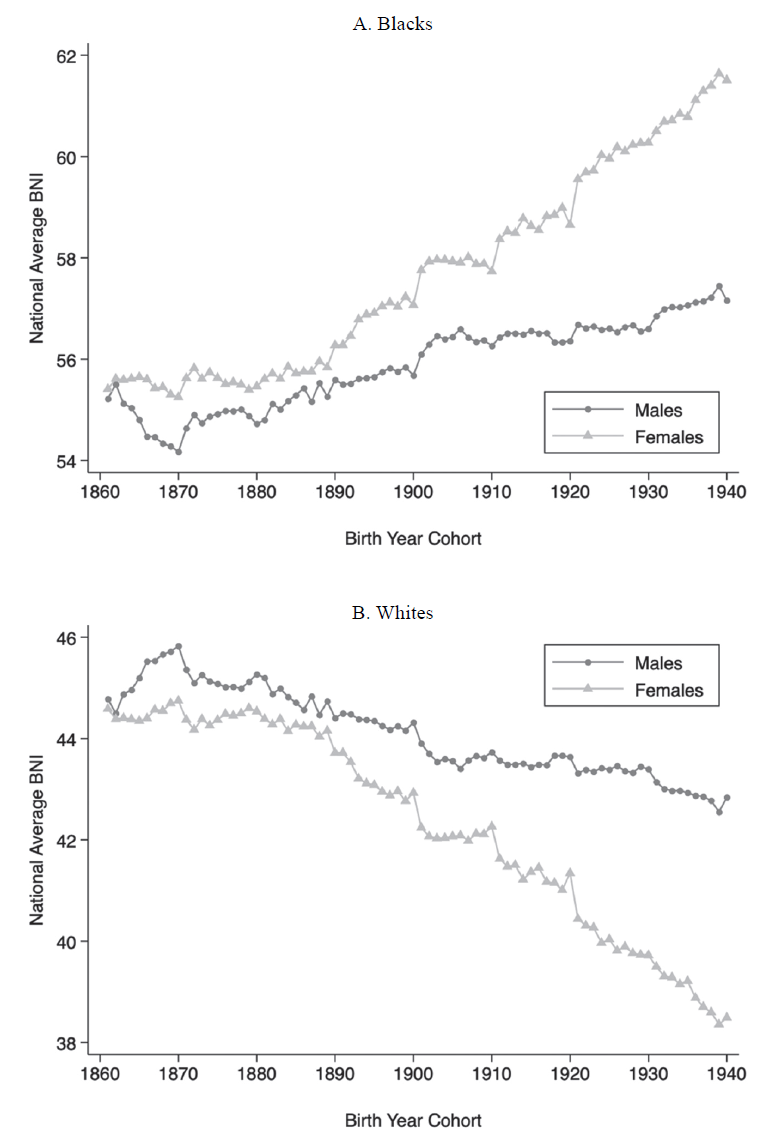
Figure 1 plots the average BNI of cohorts born between 1861 and 1940, separately by race and gender (Tan 2022).Footnote ³ Because each cohort appears in multiple censuses, only 0-to-9-year-olds are drawn from a given census year to avoid double counting.Footnote ⁴ I make three observations from Figure 1. First, racial differences in name choices were already present back in the nineteenth century. Among cohorts born in the 1860s, for example, the mean BNI was around 55 for blacks and 45 for whites. The former implies that the average black name was about 20 percent more likely to be found among blacks than whites, and vice versa for the latter. Second, these differences have widened over time.Footnote ⁵ By the 1930s, the BNI of blacks had risen by approximately 5.5 and 2.3 points for females and males, respectively, while whites moved in the opposite direction. The more pronounced shift among females could reflect a greater willingness of parents to give their daughters new or different names, as has been noted elsewhere.Footnote ⁶ This, in turn, may be facilitated by the lower likelihood of mothers passing on their names to daughters, compared with fathers giving their names to sons.Footnote ⁷ Third, the divergence in naming patterns was a relatively smooth and continuous process, with no break in trend even between cohorts that were born just before and after emancipation.Footnote ⁸

Figure 1

THE EVOLUTION OF BLACK AND WHITE NAMES

Notes: Each marker denotes the average BNI of a given cohort-gender combination, separately for blacks (A) and whites (B). To avoid double counting, cohorts are drawn by taking 0-to-9-year-olds from each census year, except in 1900, where 0-to-19-year-olds are used instead to compensate for the 1890 census.

Sources: Data are from the complete counts of the 1870 to 1940 census records, less 1890.

How do the historical patterns in Figure 1 compare with Fryer and Levitt (Reference Fryer and Levitt2004)?Footnote ⁹ As mentioned previously, Fryer and Levitt (Reference Fryer and Levitt2004) view the black-white difference in name choices as a recent phenomenon originating with the Black Power Movement of the 1970s. However, their analysis is limited to cohorts that were born after 1960. My findings suggest that had Fryer and Levitt’s (2004) series been extended further back in time, one might instead conclude that the divergence in naming patterns began much earlier.Footnote ¹⁰ Interestingly, the earliest cohorts in Fryer and Levitt’s (2004) sample of blacks, those born between 1961 and 1967, have a mean BNI of around 60.9—this is slightly higher than the latest cohorts of blacks in my data, those born in the late 1930s.Footnote ¹¹ Piecing the trends from the two studies together thus reveals a gradual and continuous evolution of naming patterns over the nineteenth and twentieth centuries, rather than an abrupt and dramatic change as proposed by Fryer and Levitt (Reference Fryer and Levitt2004).

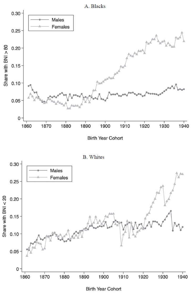
Another way of visualizing the evolution of naming patterns is to focus on the tail ends of the BNI range—names that are distinctively black or white. I consider names with BNIs over 80 to be distinctively black and names with BNIs under 20 to be distinctively white. The former are more than four times as likely to be found among blacks while the latter are more than four times as likely to be given to whites. Figure 2 then plots the share of persons that have distinctively racialized names. Three observations are worth noting here. First, the share of blacks with distinctively black names grew over time for females but not for males. The results for males, however, can be sensitive to how the raw names are cleaned, a point that I return to later. Second, the share of whites with distinctively white names rose substantially for both genders, with similar trends up until the early twentieth century, before females started to pull ahead. Third, the historical patterns for blacks can be compared against Fryer and Levitt (Reference Fryer and Levitt2004), who also trace the share of blacks with BNIs over 80 and document an increase in this share from the 1960s to the 1990s. About 15 percent of their earliest cohorts from 1961 have distinctively black names, similar to the most recent black cohorts in my sample.Footnote ¹² Putting the two series together thus reinforces the case that racial differences in names arose gradually and continuously well before the Black Power Movement.

Figure 2

SHARE WITH DISTINCTIVELY BLACK OR WHITE NAMES

Notes: Each marker denotes the share of persons in a given cohort-gender combination who have distinctively racialized names, separately for blacks (A) and whites (B). Distinctively black names have a BNI of over 80 while distinctively white names have a BNI of under 20. To avoid double counting, cohorts are drawn by taking 0-to-9-year-olds from each census year, except in 1900, where 0-to-19-year-olds are used instead to compensate for the 1890 census.

Sources: Data are from the complete counts of the 1870 to 1940 census records, less 1890.

The shift toward names that are more black or white in Figures 1 and 2 is largely robust to different ways of constructing BNI. First, I calculate BNI without converting nicknames to their proper equivalents. Figures A5 and A6 in the Online Appendix present the resulting trends in mean BNI and the share of persons with distinctively racialized names, respectively. The patterns are broadly similar to the baseline findings, except that the share of black males with distinctively black names exhibits a level shift from the 1898 cohort onward. Second, I relax the restriction on name length; rather than requiring names to have more than three characters, I drop only names that have one character. Online Appendix Figures A7 and A8 show that this does not alter the original trends. Third, I lower the threshold for name frequency from 100 individuals per name to 50. Online Appendix Figures A9 and A10 continue to display a divergence in name choices. This is also the case when the frequency threshold is completely removed, as illustrated in Online Appendix Figures A11 and A12. Fourth, to allay concerns that childhood names are simply placeholders that will subsequently be replaced as individuals grow up, I draw each cohort from a later census year and reconstruct the series in Figures 1 and 2. Specifically, I take either 10-to-19-year-olds from the 1880 to 1940 complete counts or 20-to-29-year-olds in the 1900 to 1940 censuses. Reassuringly, Online Appendix Figures A13 to A16 reveal similar trajectories in naming patterns.

Interpretation

Fryer and Levitt (Reference Fryer and Levitt2004) interpret the rise of racialized names through the lens of an identity model—is this still a valid interpretation in light of the patterns documented earlier? The identity framework posits that: (i) identities are accompanied by certain “prescriptions” which define the appropriate behavior for a particular group, such as blacks choosing distinctively black names; (ii) there is a utility benefit when one’s actions are in line with these prescriptions; and (iii) the Black Power Movement altered such identity prescriptions, causing a rapid rise in BNI during the 1970s. My historical findings, however, cast doubt on this narrative.Footnote ¹⁶ First, if Fryer and Levitt (Reference Fryer and Levitt2004) are right, then one might expect other race-related events like emancipation or black suffrage to also shift identity prescriptions abruptly, generating discontinuities or rapid changes in BNI. Instead, a relatively smooth divergence in naming patterns is observed over the period of study. Second, the growing divide in name choices stretches back to at least the mid-nineteenth century—the Black Power Movement is thus unlikely to have initiated the evolution of black and white names.

Background Literature

While the historical trends in naming patterns documented previously were based on and compared with Fryer and Levitt’s (2004) study, the contemporary nature of their work limits the insights that can be gleaned from them on the process of selecting names in the past. To understand which factors were relevant when deciding on names historically, I turn to studies that look at names in the nineteenth and early twentieth centuries. Olivetti and Paserman (2015), for instance, show that name choices in the United States vary with a father’s socioeconomic status. As an example, fathers of higher occupation standing in 1880 were more likely to name their sons “Harry” and their daughters “Bessie.” Knudsen (Reference Knudsen2022) finds that names in Scandinavia reflect how individualistic parents are. Fouka (Reference Fouka2020) observes that policies barring the German language in American schools during WWI caused German immigrants to give their children decidedly German names. Abramitzky, Boustan, and Eriksson (2020) illustrate how spending more time in the United States causes immigrants to adopt less foreign names for their offspring. Fouka, Mazumder, and Tabellini (Reference Fouka, Mazumder and Tabellini2022) conclude that the large-scale arrival of southern blacks in northern cities led European immigrants there to choose less foreign names for their children.

In the case of blacks, the process of name selection may also be influenced by a combination of ancestral origin and slavery. On the relevance of origin, Paustian (Reference Paustian1978) argues that black names in the United States have similar themes and patterns to popular names in West Africa, where the ancestors of most black Americans were from. On the role of slavery, the debate has centered on whether names were determined by slaves themselves or by their owners. Gutman (Reference Gutman1976) shows that naming conventions among slaves were used to convey some amount of familial bonding, whereas Engerman (Reference Engerman1978) notes that the party responsible for naming enslaved children is unknown.Footnote ¹⁷ Adding to this complexity, when blacks had agency over their names, either after escaping slavery or post-emancipation, their motivations for choosing a given name varied. For example, the abolitionist Sojourner Truth, born Isabella Baumfree, escaped from slavery in 1826 and changed her name in 1843 after she was convinced that God had called her to preach the truth; former slave Mollie Russell, on the other hand, took on the name “Mollie” post-emancipation simply because her sister started calling her that (Facing History & Ourselves 2015).Footnote ¹⁸

The collection of studies and examples here suggest that historically, the process of picking a name was multifaceted—it was shaped by many different forces. In the analysis that follows, I examine several such factors empirically.

Potential Determinants

I start by examining the relationship between children’s names and several characteristics of their households and counties. This is done with the following regression, separately by race:

(2) $$BN{I_{i,h,c}} = \alpha + {\zeta _1}Femal{e_{i,h,c}} + {\zeta _2}{X_{h,c}} + {\zeta _3}{X_c} + {e_{i,h,c}},$$

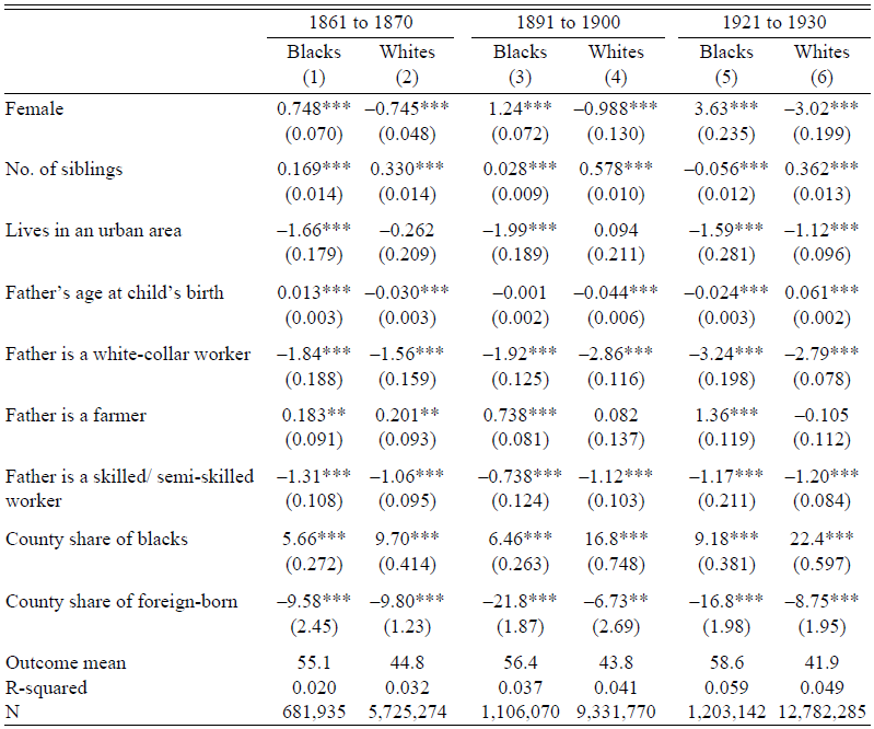
where the subscripts i, h, and c denote the child, household, and county, respectively. The indicator for females, Female, accounts for gender differences in BNI. The vector of household or parental traits, X _h,c , includes: the number of siblings a child has, a dummy for whether the household resides in an urban area, the father’s age when the child was born, and the father’s occupation category (white collar, farmer, skilled/semi-skilled). The county-level features, X _c , refer to the share of blacks and the share of foreign-born persons. For consistency with the analysis in Table 1, Specification (2) is implemented separately for three groups: the 1861 to 1870, 1891 to 1900, and 1921 to 1930 birth cohorts. Table 2 then presents the results.Footnote ¹⁹

Table 2

DETERMINANTS OF NAME CHOICES

Notes: The sample is restricted to children whose fathers have the following characteristics: they are the household head, they were 18 to 50 years old at the time of the child’s birth, and they report a valid occupation. Each column shows the coefficients from a regression of a child’s BNI on the covariates listed in the leftmost column, separately for blacks and whites, and for the three groups of cohorts listed in the column headings: the 1861 to 1870 cohorts, the 1891 to 1900 cohorts, and the 1921 to 1930 cohorts. Standard errors clustered at the county level are in parentheses.

*p < 0.1, **p < 0.05, ***p < 0.01

Sources: Data are from the complete counts of the 1870, 1900, and 1930 census records.

I make three observations from Table 2. First, in line with the gender gap noted earlier, the coefficient on the female indicator is positive for blacks and negative for whites, with the difference growing over time. Second, across race and birth years, household traits often enter Regression (2) with the same sign. Children with more siblings, who live outside urban areas, or whose fathers are farmers, tend to have higher-BNI names. That names are related to household characteristics may not be surprising, given the findings in Olivetti and Paserman (2015) and Knudsen (Reference Knudsen2022) mentioned earlier. More interesting, perhaps, is the third observation: there is a strong connection between a child’s name and the demographic makeup of a county. Those residing in areas with relatively more blacks or few immigrants are given names that have higher BNIs. This hints at the possibility of natives being influenced by the types of people living around them, complementing Fouka, Mazumder, and Tabellini’s (2022) observation that immigrants adopt less foreign names for their children in response to black migrants arriving from the South. While not causal, these patterns suggest that the location of residence may affect name choices, over and above household-level determinants.

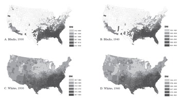
Further insights into the role of place can be gained by studying the geography of names. I proceed by averaging the BNI of non-Hispanic natives aged 20 and under in a given county, separately for blacks and whites. This is done with the 1930 and 1940 censuses as relatively few blacks lived outside the South prior to the first Great Migration, limiting the geographic scope in earlier years. For greater accuracy, I also restrict the focus to counties with at least 100 persons in the corresponding race-year combination. Figure 3 then maps the mean BNI in each of these counties, by race and year. Darker shades indicate areas where children tend to have higher-BNI names, though this has a subtly different interpretation for blacks and whites as they have different BNIs on average— blacks in these locations have names that are more black while whites in such places have names that are less white.

Figure 3

THE GEOGRAPHY OF NAMES

Notes: The subfigures show the mean BNI among 0-to-20-year-old non-Hispanic natives in each county, separately for blacks (A and B) and whites (C and D). For greater accuracy, the sample is restricted to counties with at least 100 persons in a given race-year combination. The sample sizes are 1,526 (A), 1,487 (B), 3,093 (C), and 3,091 (D) counties.

Sources: Data are from the complete counts of the 1930 and 1940 census records.

I find substantial variation in naming patterns across the country. For blacks, the mean county BNI ranges from a low of around 40 to a high of about 65 (Figures 3A and B). Blacks in the former tend to have names that are more likely to be found among whites, while those in the latter have names that are almost twice as likely to be given to blacks. For whites, the average county BNI goes from about 33 to 55 (Figures 3C and D). Mirroring the patterns for blacks, whites in the former have names that are twice as likely to be used by whites, while those in the latter have names that are slightly more likely to be associated with blacks. Importantly, there is a distinct regional component to the geography of names for both blacks and whites: individuals residing outside the South have names with lower BNIs than those within the South.Footnote ²⁰ More precisely, blacks in the non-South are given names that are less black than their counterparts in the South, while whites outside the South receive names that are more white than those in the South.

While suggestive of a role for place, the geographic divide in names could also reflect selective migration. In particular, households that prefer lower-BNI names may be more likely to settle outside the South. The subsections that follow explore both possibilities in turn.

Selective Migration

Is the link between geography and names partly driven by selective migration? To investigate this, I divide children into two groups: those born within and outside the South. For each group, I consider children who are still living in their birth regions to be stayers and those that are not to be migrants.Footnote ²¹ I then ask if naming patterns differ by migration status. This is quantified with the following regression, separately by birth region, race, and census year:

(3) $$BN{I_i} = \alpha + {\beta ^{mig}}Migran{t_t} + FE + {\varepsilon _i},$$

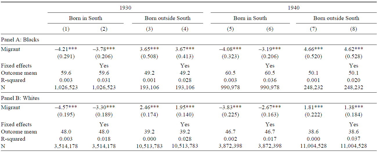
where Migrant is an indicator for children who left their region of birth and FE is a vector of fixed effects for gender, birth year, birth order, and birth state. The parameter β ^mig captures the average difference in BNI between migrants and stayers. For selective migration to explain the geographic divide in naming patterns (Figure 3), β ^mig should be negative for the subset of southern-born children and positive for their counterparts born outside the South.

Table 3 presents the results from implementing Regression (3) on the sample of children aged 20 or younger in the 1930 and 1940 censuses. Odd columns provide the basic estimates, while even columns include the full set of fixed effects. As predicted, the coefficient on migration status is negative for southern-born children and positive for children born outside the South. Individuals leaving the South thus come from households with a preference for lower-BNI names, while those entering the South are from families that tend to use higher-BNI names. This pattern is observed across races, census years, and specifications. The BNI differentials are also sizable in magnitude at around 4 to 10 percent of the mean BNI. Such differences, particularly between southern-born migrants and stayers, may complement the broader literature on the Great Migration. Collins and Wanamaker (Reference Collins and Wanamaker2014, Reference Collins and Wanamaker2015), for instance, find that blacks and whites who moved to the North during the first Great Migration were positively selected along a range of characteristics, including occupation status and homeownership. My results indicate a related dimension of sorting: naming patterns.Footnote ²² Taken as a whole, Table 3 suggests that at least part of the spatial variation in names is driven by selective migration.

Table 3

SELECTIVE MIGRATION AND NAME CHOICES

Notes: The sample is restricted to non-Hispanic natives aged 0 to 20 who were born in the South (Columns (1), (2), (5), and (6)) or born outside the South (Columns (3), (4), (7), and (8)). For households with multiple children, one child is randomly selected to be part of the sample. Each cell shows the coefficient from a regression of a child’s BNI on migrant status, where the latter is an indicator for those who left their region of birth. Even columns include a vector of fixed effects for gender, birth year, birth order, and birth state. Standard errors clustered at the destination county level are in parentheses.

*p < 0.1, **p < 0.05, ***p < 0.01

Sources: Data are from the complete counts of the 1930 and 1940 census records.

The Role of Place

Beyond selective migration, could the place of residence itself also contribute to the association between location and name choices? This subsection attempts to isolate the causal effect of place by exploiting the migration of households across regions.

To implement the migration research design, I focus on households that left the South and ask if there are systematic differences in naming patterns between siblings born before and after the move—information on the year of migration is thus required.Footnote ²³ This is not directly available in the historical censuses, which are cross-sectional and contain few questions on migration history. Instead, I make use of differences in the region and year of birth among siblings to infer when a household moved. Drawing once again on census data from 1930 and 1940, I start by identifying households that (i) have two or more children, (ii) where at least one child was born in the South and at least one was born outside the South, and (iii) where there is a monotonic transition from being born in the South to being born outside the South as one goes from the oldest to the youngest child.Footnote ²⁴ The first two criteria isolate households that moved across regions, while the third restricts the sample to households that are likely to have moved just once. For this set of households, I then order siblings by age, identify the adjacent siblings with different birth regions, and take the midpoint of their birth years to be the household’s year of migration.Footnote ²⁵ For concreteness, consider a family with six children in 1930: Curline (born 1918 in the South), Joseph (born 1920 in the South), Marguerite (born 1921 in the South), Ruth (born 1923 in the South), Jean (born 1925 outside the South), and Selma (born 1928 outside the South).Footnote ²⁶ Ruth and Jean are adjacent siblings born in different regions. Based on their birth years, this house-hold’s year of move will be imputed as 1924. Similar approaches have also been used in other work (Atack and Bateman Reference Atack and Bateman1987; Bazzi, Fiszbein, and Gebresilasse Reference Bazzi, Fiszbein and Gebresilasse2020; Collins and Zimran Reference Collins and Zimran2019). This procedure, however, can only be applied to households that meet the three criteria—caution is thus necessary when extrapolating the results here to the general population.Footnote ²⁷

With the sample of movers and information on when they moved, I then estimate an event study specification to determine the causal effect of place on name choices:

(4) $$BN{I_{i,h}} = \alpha + \sum\limits_{m = - 10}^{m = 10} {{\beta _m}1{{[{\rm{Years}}\,{\rm{Since}}\,{\rm{Move}} = m]}_{i,h}} + {\theta _h} + {X_{i,h}} + } {\varepsilon _{i,h}},$$

where much of the notation follows from before. The outcome is the BNI of a child’s name, while the main explanatory variable is a set of indicators for the number of years since a household moved at the time the child was born, m, calculated by subtracting the household’s migration year from the child’s birth year. Births before the migration event thus have negative values of m, whereas births after the move have positive values.Footnote ²⁸ For simplicity, births occurring more than 10 years before or after a household migrated are coded as m = –10 and m = 10, respectively.Footnote ²⁹ To isolate within-household changes in naming patterns, household fixed effects, θ _h, are added to the regression. These account for household-specific preferences over names, but there may still be potential confounders within households. A vector of individual-level controls, X _i,h, is thus included to complete the specification: gender, birth order, and birth year in decade bins.Footnote ³⁰ If place matters for name choices, one should expect the trend in β _m to exhibit a distinct break post-move.

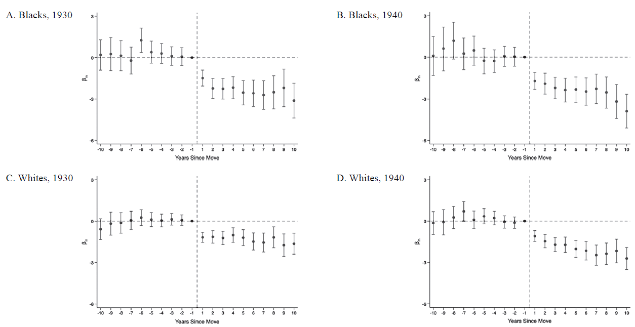
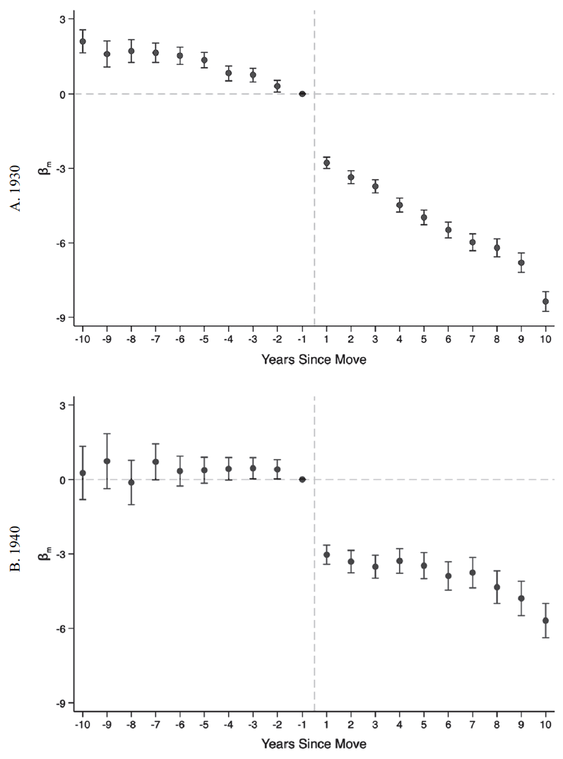
Figure 4 presents the estimates of β _m from Regression (4), by race and census year. Standard errors clustered at the household level are used to construct 95 percent confidence intervals. Children born a year before their households moved form the reference group—each coefficient thus captures the average difference in BNI between a child and the sibling born just before the migration occurred.

Figure 4

EVIDENCE FOR PLACE EFFECTS ON NAME CHOICES

Notes: The sample is restricted to children aged 20 and under from households that left the South. The markers in each subfigure denote the coefficients β_m from a regression of a child’s BNI on a vector of indicators for the number of years since a household moved at the time the child was born, controlling for household fixed effects, gender, birth order, and birth year in decade bins. Children born a year before their households moved are the reference group. 95 percent confidence intervals are displayed, based on standard errors clustered at the household level. The sample sizes are 98,018 (A), 97,641 (B), 277,574 (C), and 270,003 (D).

Sources: Data are from the complete counts of the 1930 and 1940 census records.

There are three key takeaways from Figure 4. First, the pre-move β _m estimates are mostly insignificant and fluctuate in sign, indicating that siblings born before their households moved have names with relatively similar BNIs. There is thus no trend toward higher-or lower-BNI names in the lead up to a household’s departure from the South. Second, a distinct break in naming patterns is observed post-migration, with the β coefficients becoming significant and consistently negative.Footnote ³¹ This is evident for both blacks and whites—black children born after their households moved tend to be given names that are less black compared with their older siblings, whereas their white counterparts receive names that are more white. Third, there is some evidence that the shift in name choices increases with time spent outside the South. Fitting best-fit lines to the post-move estimates yields gradients of –0.105 (S.E.=0.034), –0.184 (S.E.=0.035), –0.061 (S.E.=0.019), and –0.154 (S.E.=0.020) for Figures 4A, B, C, and D, respectively. These imply that an additional year of exposure to the non-South lowers the BNI of names given to children by 0.061 to 0.184 points. Such patterns may be consistent with other work. Bazzi, Fiszbein, and Gebresilasse (Reference Bazzi, Fiszbein and Gebresilasse2020), for example, show that families are more likely to choose individualistic names for their children the longer they stay on the American frontier; Chetty and Hendren (Reference Chetty and Hendren2018) find that each extra year of childhood spent in a better loca tion improves a person’s adult income rank. The level shift and subsequent trend in BNI after migration can also be observed when replacing the years-since-move indicators in Regression (4) with a post-move dummy and its interaction with the number of years since moving, as Table A5 in the Online Appendix shows. This model indicates a decline in BNI by 1.10 to 1.77 points after migrating, followed by a further drop of 0.082 to 0.142 points per year spent outside the South. Taken together, the evidence suggests that place affects how parents name their children.

My findings are robust to further controlling for secular trends in name choices. I illustrate this in two ways. First, instead of dividing birth years into decade bins, I use 5-year bins to better account for any underlying changes in naming patterns.Footnote ³² Figure A20 in the Online Appendix shows that this does not alter the baseline results substantially. Second, I control for pre-move-state trends in names.Footnote ³³ These are captured by the mean BNI for each state-cohort-gender combination, based on children from households that remained in the South.Footnote ³⁴ Online Appendix Figure A21 reveals that the original findings are not significantly affected by this adjustment.

Can the post-migration shift in name choices be attributed to the causal effect of place? I consider several potential threats to such an interpretation.

A key assumption underlying the event study framework is that parents would not have changed how they name their children had the household remained in the South. While this counterfactual cannot be observed, the insignificant pre-move estimates in Figure 4 suggest that naming patterns are likely to have continued along the same path if the household had not migrated. The identifying assumption thus appears to be reasonable.

Another issue is whether the post-migration break in naming patterns reflects some shock that simultaneously causes households to leave the South and to give their children different names. In particular, could income shocks cause households to move and shift their preferences toward lower-BNI names, biasing the estimates of place effects upward? I provide three reasons why this is unlikely to be the case. First, while both positive and negative income shocks can lead to departures from the South, it is unclear if these opposite forces will also alter name choices in the same direction.Footnote ³⁵ Second, even if income shocks can explain the jump in β _m around the time of the move, it is still difficult to connect such low-frequency events to the continued decline in BNI post-migration. Third, reasonably comparable place effects can be observed for house-holds from different parts of the South even though the shocks they experience in their origins are likely to differ substantially. Taking inspiration from the Great Migration literature, southern push factors depend on the types of crop being grown, while pull factors from outside the South have varying degrees of influence on each southern location because of pre-existing South-to-non-South migration networks (Boustan Reference Boustan2010, Reference Boustan2016; Derenoncourt Reference Derenoncourt2022). This suggests that the event study estimates should vary by household origin if the baseline results are indeed driven by confounding shocks. To test this, I run Regression (4) separately for those from southern states where the percent of acreage in cotton is above or below 90. Reassuringly, I do not find large differences in place effects between the two groups (Figures A22 and A23 in the Online Appendix).

I also check if the baseline results are driven by systematic differences between the names of first-borns and their younger siblings, the former of which are in the pre-move period by construction. If first-borns tend to be named after their parents or ancestors, and if those names have higher BNIs on average, this might generate the patterns in Figure 4. Birth order controls alone may not fully account for such differences. To make progress, I restrict the sample to households that had at least two children before leaving the South, drop first-borns entirely, and then rerun Regression (4). Figure A24 in the Online Appendix illustrates that similar conclusions can be reached even with this subset of movers. A more general problem, however, could arise if family naming conventions apply not just to first-borns but to subsequent children as well. I address this in two ways. First, I show in Online Appendix Tables A6 and A7 that there is no consistent evidence of BNI declining with birth order, based on the sample of southern stayers. This implies that name differences by birth order are unlikely to explain the baseline results. Second, I repeat the event study analysis separately for smaller (less than five children) and larger (five or more children) households. Smaller households are less likely to have exhausted the available set of family names—little effect should thus be seen among them if the baseline findings were due to the switch from family to non-family names. Instead, Online Appendix Figures A25 and A26 indicate that place effects can be observed for both groups.

To further allay concerns that my results might reflect some confounding factor, I implement a placebo test. Taking households that remained in the South, I randomly assign each of them an artificial year of move and then run the baseline analysis on these stayers instead of movers. Figure A27 in the Online Appendix shows no effect of place on name choices—all the year- of-move coefficients are small in magnitude and statistically insignificant.

I conclude this section by exploring whether place effects vary by gender, local naming patterns, and racial residential segregation.

First, I run Regression (4) separately for females and males. Figures A28 and A29 in the Online Appendix present the corresponding results. The estimates are less precise than those in Figure 4, but a similar pattern can still be observed for the most part: largely insignificant coefficients in the pre-move period followed by negative and significant effects post-move, for both genders. I find that the level shift in BNI—based on the average size of the post-migration β _m s—is somewhat larger for females, possibly reflecting the greater willingness of parents to give their daughters different names (Russo Reference Russo2020; Sue and Telles Reference Sue and Telles2007). However, gender differences in the post-move trend in place effects—based on the gradient of best-fit lines to the post-migration β _m s—paint a less consistent picture that varies by race and census year.

Next, I investigate if the impact of the surrounding environment depends on local naming patterns. This is done by dividing households into two groups, based on whether the race-specific mean BNI in their non-South county of residence is above or below the median, and then implementing Regression (4) for each group. Online Appendix Figures A30 and A31 display the corresponding results. Place effects can be observed for both groups, but the differences between them are not large. This could reflect the narrower spread in mean county BNI outside the South compared with the differences between the South and non-South.Footnote ³⁶

Finally, I ask if the importance of place varies with the degree of racial segregation.Footnote ³⁷ Mirroring the previous analysis, I run Regression (4) separately for children in more (above-median) or less (below-median) segregated non-South counties.Footnote ³⁸ Online Appendix Figures A32 and A33 provide the results.Footnote ³⁹ The post-move β coefficients are broadly comparable for both groups, while differences in the trends traced out by the post-move β _m estimates again depend on the specific race and year. There is therefore little consistent evidence that segregation affects the strength of place effects. This potentially ties in with Fryer and Levitt (Reference Fryer and Levitt2004), who observe a sizable relationship between segregation and distinctively black names among blacks by the 1970s but less so in the early 1960s.Footnote ⁴⁰

Improvements in Household Economic Status

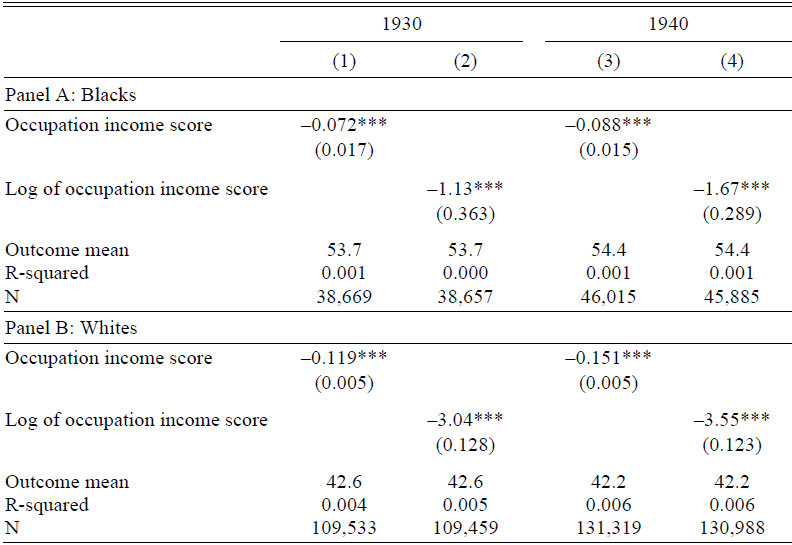
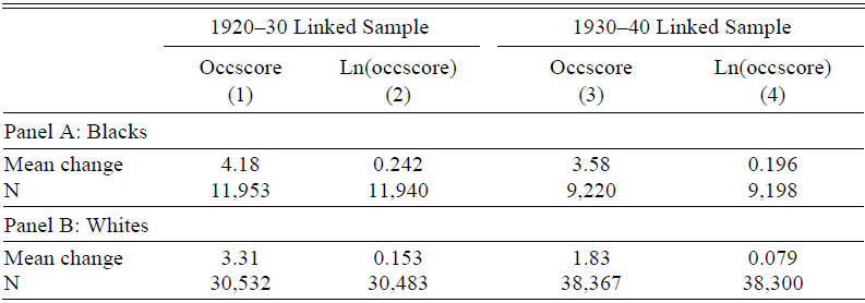
Collins and Wanamaker (Reference Collins and Wanamaker2014, Reference Collins and Wanamaker2015) find substantial economic gains to leaving the South in the early twentieth century—could this have shifted parents’ preferences in favor of lower-BNI names? If such gains accumulate with time spent outside the South, this hypothesis may explain not just the break in naming patterns around the time of the move, but the post-migration trend in place effects as well. I argue that this is a plausible but incomplete story. A three-step back-of-the-envelope calculation can be used to illustrate this. First, I estimate the relationship between children’s names and the economic status of their households. This is done by regressing a child’s BNI on the level or log occupation income score of the household head, using only children who were born after their households left the South.Footnote ⁴¹ A strong negative association is observed across race and census years, as shown in Table 4. Second, I calculate the average economic gains after migration. To do this, I link 20-to-40-year-old native-born men from the 1920 and 1930 censuses to their older selves in the 1930 and 1940 records, respectively. I then keep those who migrated out of the South during the decade interval and compute the change in their economic status. Table 5 reveals positive gains for both blacks and whites. Third, I combine the results from the previous steps, multiplying the improvements in Table 5 (migration to economic status) with the correlations in Table 4 (economic status to names). This yields effects (migration to names) that are similar in direction but smaller in size compared with the post-move β _m estimates in Figure 4. The back-of-the-envelope calculation thus suggests that while there may be a role for economic improvements, other important factors are also at play.

Table 4

CHILDREN’S NAMES AND HOUSEHOLD ECONOMIC STATUS

Notes: The sample is restricted to children aged 20 and under from households that left the South, who were born after their households moved, and whose fathers are native-born household heads with non-missing information on occupations. Each cell shows the coefficient from a regression of a child’s BNI on either the household head’s occupation income score (odd columns) or log occupation income score (even columns). Standard errors are in parentheses.

*p < 0.1, **p < 0.05, ***p < 0.01

Sources: Data are from the complete counts of the 1930 and 1940 census records.

Table 5

ECONOMIC GAINS AFTER LEAVING THE SOUTH

Notes: The base population comprises 20-to-40-year-old native-born men. The linked samples are then restricted to those who lived in the South during the initial year but were residing outside the South in the later census, who were household heads in both years, and who were not in school in either year. Each cell shows the average change in economic status over the decade interval, where economic status is measured by the level or log occupation income score (“occscore”).

Sources: Data are from the 1920–30 and 1930–40 linked samples.

The Return to Names

Could the post-migration shift in naming patterns be a response to regional differences in the return to names instead? If lower-BNI names carry greater benefits outside the South, parents may be incentivized to select names that are less black or more white to maximize the lifetime earnings of their children. These returns can either be perceived—that is, parents draw their conclusions from simply observing how successful individuals with a given name are—or real—that is, names have a causal effect on life outcomes. I explore both possibilities in turn.

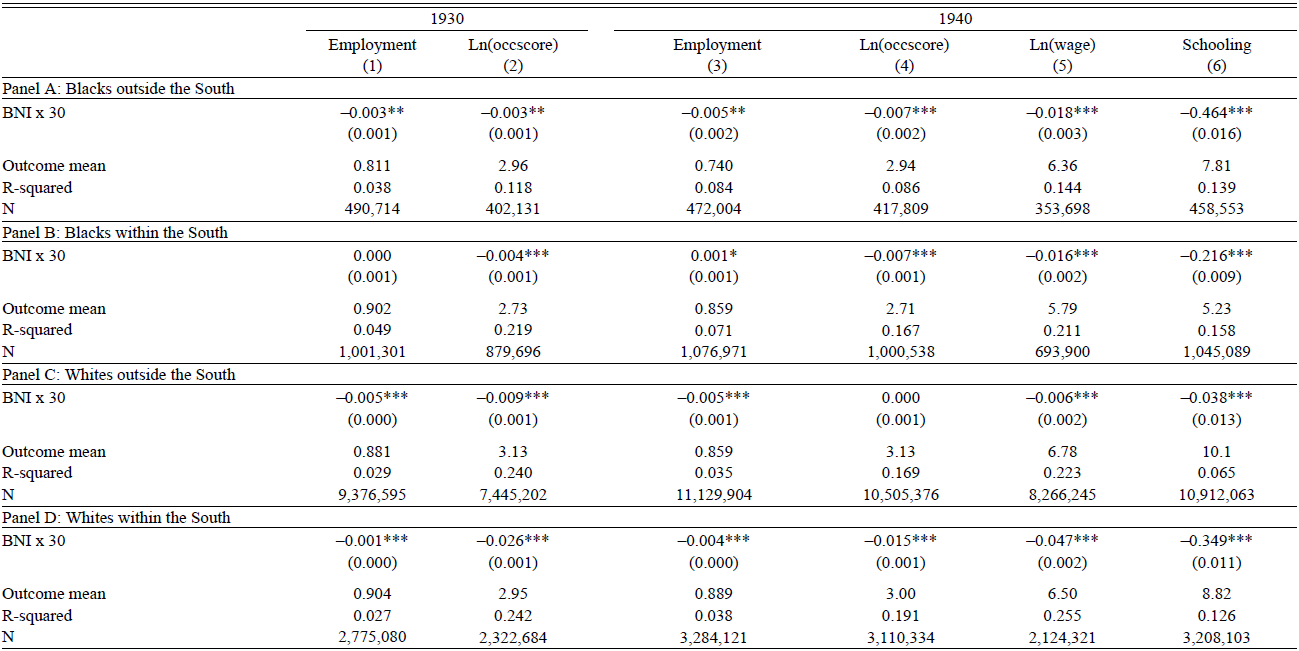
Do individuals with lower-BNI names fare better economically, especially outside the South? While such associations need not be causal, they could still shape parental perceptions of how different names are rewarded. In the case of France, for example, Algan et al. (Reference Algan, Malgouyres, Mayer and Thoenig2022) show that local information on the unemployment differential between those with Arabic and non-Arabic names strongly influences whether parents give their children Arabic names. I proceed by considering the relationship between names and several socioeconomic outcomes for 20-to-40-year-old natives in 1930 and 1940. Given the large gender gap in labor force participation at the time (Boustan and Collins Reference Boustan and Collins2014), a different set of outcomes will be used for each gender.

I begin by analyzing the outcomes for men with the following model:

(5) $${Y_{i,c}} = \alpha + {\beta ^{perceived}}BN{I_{i,c}} + Ag{e_{i,c}} + {\theta _c} + {u_{i,c}},$$

where Y refers to a given outcome, Age is individual i’s age, and θ _c represents a vector of fixed effects for each county c. The outcomes of interest are: employment status, the log of occupation income scores, the log of wages, and years of schooling, the latter two of which are only available in 1940. Table 6 presents the corresponding β ^perceived estimates by race, region, and year, all scaled to reflect a 30-point shift in BNI. Assuming linearity, the scaled results may then be interpreted as the difference in outcomes when comparing a name that is equally likely to be held by blacks and whites (BNI of 50) to one that is four times as likely to be given to blacks (BNI of 80), or when switching from a name that is four times as likely to be found among whites (BNI of 20) to one that both races are just as likely to use (BNI of 50).

Table 6

THE ASSOCIATION BETWEEN NAMES AND OUTCOMES FOR MEN

Notes: The sample is restricted to non-Hispanic native-born males aged 20 to 40 who are not in school. The sample in Column (5) is further restricted to wage and salary workers. Each cell shows the scaled coefficient from a regression of one of the outcomes listed in the column headings on the BNI of an individual’s name, controlling for age and county fixed effects. The raw coefficients are scaled to reflect a 30-point shift in BNI. The term “occscore” refers to occupation income scores. Standard errors clustered at the county level are in parentheses.

*p < 0.1, **p < 0.05, ***p < 0.01

Sources: Data are from the complete counts of the 1930 and 1940 census records.

Table 6 reveals three things about the perceived return to names. First, men with higher-BNI names tend to do worse in the labor market. Second, however, these correlations are relatively small in magnitude. Among blacks living outside the South in 1940, for example, a 30-point increase in BNI is associated with a 2 percent decline in wages. While there is a stronger link between names and human capital, this does not translate into large earnings differentials, possibly due to the lower return to schooling in the mid-twentieth century compared with more recent times (Feigenbaum and Tan 2020). Third, there is no consistent evidence that lower-BNI names carry greater benefits outside the South. The non-South associations are comparable to or more negative than those in the South for blacks (Panels A versus B), but the correlations are typically stronger within the South for whites (Panels C versus D). This contrast, when juxtaposed against the consistent direction of place effects for both blacks and whites (Figure 4), suggests that regional differences in the perceived return to names are unlikely to be driving the post-migration change in name choices.

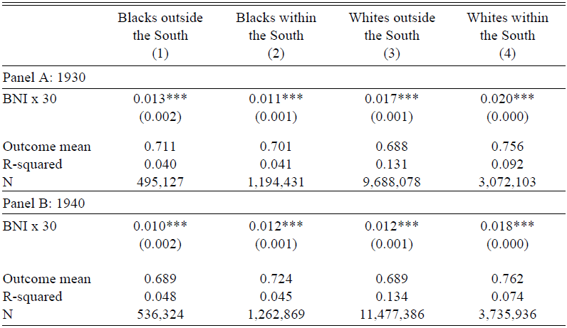
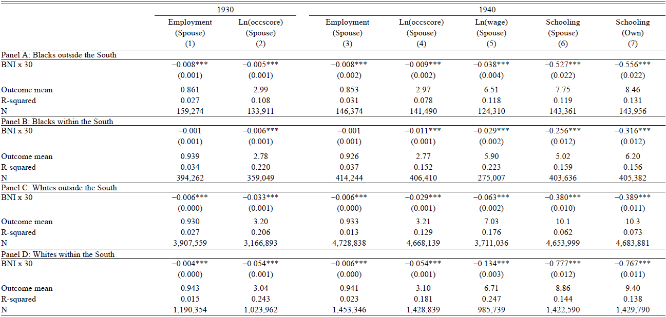
Next, I explore the perceived return to names for women. This is done in two steps. First, I ask if there is a link between the BNI of names and marital status. Table 7 shows the results from running Regression (5) with an indicator for married persons as the outcome. Women who have higher-BNI names are more likely to be married. If marriage is viewed as a “positive return,” then the estimates here go in the opposite direction of that needed to generate the shift in Figure 4. In any case, the difference in marriage propensity associated with a 30-point increase in BNI is small, never exceeding 3 percent of the average marriage rate. Second, I narrow the focus to married women and ask if their names are related to the economic status of their husbands, again using a specification similar to Regression (5). Table 8 presents the corresponding associations, mirroring the outcomes and layout in Table 6. Women with more-black or less-white names tend to have husbands with lower economic status, part of which could be due to assortative mating. Columns (6) and (7) provide evidence for this by looking at the educational attainment of husbands and wives; both are negatively related to the wife’s BNI.

Table 7

THE ASSOCIATION BETWEEN NAMES AND MARITAL STATUS FOR WOMEN

Notes: The sample is restricted to non-Hispanic native-born males aged 20 to 40 who are not in school. The sample in Column (5) is further restricted to wage and salary workers. Each cell shows the scaled coefficient from a regression of one of the outcomes listed in the column headings on the BNI of an individual’s name, controlling for age and county fixed effects. The raw coefficients are scaled to reflect a 30-point shift in BNI. The term “occscore” refers to occupation income scores. Standard errors clustered at the county level are in parentheses.

*p < 0.1, **p < 0.05, ***p < 0.01

Sources: Data are from the complete counts of the 1930 and 1940 census records.

Table 8

THE ASSOCIATION BETWEEN NAMES AND OUTCOMES FOR MARRIED WOMEN

Notes: The sample is restricted to non-Hispanic native-born married women aged 20 to 40, who are living with their husbands and whose husbands satisfy the aforementioned demographic criteria and are not in school. The sample in Column (5) is further restricted to those whose husbands are wage and salary workers. Each cell shows the scaled coefficient from a regression of one of the outcomes listed in the column headings on the BNI of the wife’s name, controlling for her age and county fixed effects. The raw coefficients are scaled to reflect a 30-point shift in BNI. The term “occscore” refers to occupation income scores. Columns (1) to (6) focus on the husband’s outcomes (“spouse”), while Column (7) looks at the wife’s outcome (“own”). Standard errors clustered at the county level are in parentheses.

*p < 0.1, **p < 0.05, ***p < 0.01

Sources: Data are from the complete counts of the 1930 and 1940 census records.

Women who are given higher-BNI names thus complete fewer years of schooling and also marry men who have less human capital. Crucially, when considering the full range of outcomes, regional differences in the respective associations again differ by race—they are typically stronger outside the South for blacks but within the South for whites. This inconsistency suggests that the place effects in Figure 4 do not reflect parental responses to geographic differences in the perceived value of names.

Beyond the observed correlations, do names have a causal effect on economic outcomes and does this effect vary systematically across regions? In more recent settings, Bertrand and Mullainathan (Reference Bertrand and Mullainathan2004) find that white names receive 50 percent more callbacks for interviews than black names; Fryer and Levitt (Reference Fryer and Levitt2004), however, conclude that black names have little adverse effects once a person’s background characteristics are accounted for. Further back in the early twentieth century, Goldstein and Stecklov (Reference Goldstein and Stecklov2013) document a negative association between distinctively black names and occupational status. The mixed evidence motivates a fresh look at the return to names.

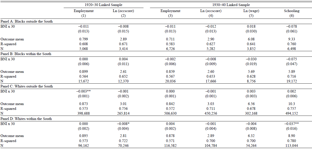
With the exception of audit studies, existing work on the return to black and white names is likely to suffer from omitted variable bias. Fryer and Levitt (Reference Fryer and Levitt2004) and Goldstein and Stecklov (Reference Goldstein and Stecklov2013), for instance, are limited to OLS regressions with observable controls. To improve on this, I compare the outcomes and names of siblings, thus accounting for potential confounders at the household level. The data for such an exercise are obtained by linking 10-to-20-year-old boys from the 1920 and 1930 censuses to their older selves in 1930 and 1940, respectively. This age range ensures that individuals are young enough to be living with their siblings in the earlier census—thus allowing one to identify brothers— but also old enough to be in the labor market by the later census. For simplicity, I further restrict the sample to households where exactly two sons can be linked. The within-household analysis can then be implemented with the following regression:

(6) $${Y_{i,h}} = \alpha + {\beta ^{actual}}BN{I_{i,h}} + Ag{e_{i,h}} + {\theta _h} + {u_{i,h}},$$

which replaces the vector of county fixed effects in Specification (5) with childhood household fixed effects. Of course, this approach does not deal with confounders within households, but the degree of bias is likely to be smaller than that in current observational studies.

Table 9 presents the β ^actual estimates from Regression (6), scaled to reflect a 30-point change in BNI. Following the analysis of perceived returns, I focus on employment status, the log of occupation scores, the log of wages, and years of schooling as the outcomes. To shed light on regional heterogeneity, I also divide the samples into those residing outside the South in 1930 and 1940 (Panels A and C) and those living in the South over both periods (Panels B and D). I find that names have little effect on labor market outcomes, with most of the point estimates being close to zero and statistically insignificant. Importantly, the null effect is observed across regions. That is, names do not appear to matter within or outside the South. Table A8 in the Online Appendix shows that broadly similar conclusions can be reached when the sample is limited to brothers who are no more than two years apart, between whom differences in unobserved characteristics may be smaller. These findings suggest that the post-migration change in naming patterns depicted in Figure 4 is unlikely to be a response to regional differences in the return to names.

Table 9

THE RETURN TO NAMES

Notes: The base population comprises 10-to-20-year-old native-born males. The linked samples are further restricted to non-Hispanics from households where exactly two sons of the household head can be linked, both of whom were not in school during the later census. Columns (2) and (4) are restricted to households where both sons had positive occupation scores in the later census year. Column (5) is restricted to households where both sons were wage and salary workers in 1940. Panels A and C refer to those who were outside the South in both the initial and later censuses, while Panels B and D focus on those who remained in the South over both decades. Each cell shows the scaled coefficient from a regression of one of the outcomes listed in the column headings on the BNI of an individual’s name, controlling for age and childhood household fixed effects. The raw coefficients are scaled to reflect a 30-point shift in BNI. The term “occscore” refers to occupation income scores. Standard errors clustered at the childhood household level are in parentheses.

*p < 0.1, **p < 0.05, ***p < 0.01

Sources: Data are from the 1920–30 and 1930–40 linked samples.

Cultural Assimilation

Thus far, the focus has been on economic-related explanations for the post-migration shift in naming patterns—is there a role for cultural assimilation instead? Intuitively, being exposed to a new environment with a different way of life can influence one’s behavior, causing a person to become more like those in the surrounding community. Measuring this cultural change among migrant households, however, is challenging because information on cultural practices is not systematically collected. Names have often been used to proxy for culture in the economic history literature (Abramitzky Boustan, and Eriksson 2020; Knudsen Reference Knudsen2022), but they are already the outcome of interest in this paper. I thus turn to inter-marriage rates as an alternative metric, here defined as marriages between two parties born in different regions.Footnote ⁴³ This assumes that there are cultural differences across regions, even within the same race.Footnote ⁴⁴ Elsewhere, inter-marriage rates have also been used to study the assimilation of immigrants (Fouka, Mazumder, and Tabellini Reference Fouka, Mazumder and Tabellini2022; Mazumder Reference Mazumder2019).

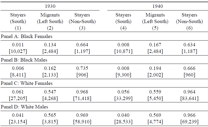
To shed light on the relevance of cultural assimilation, I proceed in two steps. First, I identify several groups of married natives aged 20 to 40 in 1930 and 1940: (i) southern-born persons living in the South (stayers), (ii) southern-born individuals residing outside the South (migrants), and (iii) those who were born outside the South and that remain there (stayers). Second, for each group, I compute the share of persons who have non-southern-born spouses. Without assimilation, intermarriage rates should be similar for both southern-born stayers and migrants, conditional on marriage. With assimilation, higher intermarriage rates might be expected among migrants instead, again conditional on marriage. Table 10 shows that the proportion of movers having non-southern-born spouses lies between that of South and non-South stayers, the latter of which provides an upper bound. While not causal, these patterns suggest that migrants may be assimilating into their new surroundings, a development that could explain the shift in name choices.Footnote ⁴⁵

Table 10

SHARE OF MARRIED PERSONS WITH SPOUSES BORN OUTSIDE THE SOUTH

Notes: The samples are restricted to 20-to-40-year-old non-Hispanic native-born married persons, excluding those who were born in or are currently residing in Alaska or Hawaii. “Stayers (South)” are defined as those who were born in the South and are still residing in the South. “Migrants (left South)” are defined as those who were born in the South but are no longer residing in the South. “Stayers (non-South)” are defined as those who were born outside the South and are still residing outside the South. Each cell shows the share of individuals in a given subgroup who are married to a person born outside the South. Sample weights are used for all computations. Sample sizes are in brackets.

Sources: Data are from the 1930 and 1940 IPUMS samples.