2. MODEL DESCRIPTION

We consider an M/G/1 queue with a workload-dependent service rate. The customers (or jobs) arrive according to a Poisson process of rate λ. The service requirement of the nth customer is B_n, n = 1,2,…, where the B_n are assumed to be independent and identically distributed (i.i.d.) copies of a random variable B with distribution B(·) and mean β. We also assume that the sequences of interarrival intervals and service requirements are independent.

The server works at a rate that depends on the amount of work in the system as described by some function r(·); that is, the service rate is r(x) when the amount of work is x. As in [1,2,9], we assume that r(0) = 0 and that r(·) is strictly positive and left-continuous and has a right limit on (0,∞). In addition, we specifically focus on the case that r(·) is increasing on (0,r_max] and decreasing on (r_max,∞) for some r_max ≥ 0.

The admission of work into the system is governed by a control policy that prescribes whether arriving customers are accepted or rejected, depending on the state of the system. We assume that the service requirement of a customer only becomes known after the acceptance decision; see Section 7 for a further discussion. Thus, the admission control policy might equivalently be interpreted as a rule for closing or opening access to the system.

We seek an admission control policy that maximizes the long-run throughput. The long-run throughput under policy π is defined as

assuming the limit to exist. Here B^π(0,t) denotes the amount of work completed during [0,t] under policy π. A policy π* is said to be (strictly) optimal if TH^π* ≥ TH^π (TH^π* > TH^π) for all policies π ≠ π*.

For now, we restrict the attention to the class of stationary and deterministic policies that base their actions on the current amount of work in the system only. For a given policy π, we use π(x) = 1 to denote that it accepts a customer that arrives when the workload equals x and write π(x) = 0 otherwise. Later we will show that the found optimal policy is in fact optimal within a broader class that includes nonstationary and randomized policies as well.

Let V_t^π be the workload at time t and let W_n^π be the workload just before the nth arrival epoch. Denote by V^π and W^π the random variables with the corresponding steady-state distributions, if they exist, and let v^π(·) be the density of V^π.

We first consider the case λβ < r_∞, with r_∞ := lim_x→∞ r(x). In that case, the system remains stable under the greedy policy that always accepts customers. Thus, the throughput achieved under the latter policy equals λβ, which is optimal, since the maximum achievable long-run throughput is bounded by the offered traffic load.

In the remainder of the article we focus on the case λβ > r_∞. (The boundary case λβ = r_∞ is rather delicate, and a full analysis is beyond the scope of the present article.) In that case, the system is unstable under the greedy policy that always accepts customers. Henceforth, we restrict the attention to policies π such that π(x) = 0 for all x > M for some large M, which ensures the existence of the steady-state workload distribution. Even though the policy that always accepts customers might continue to be optimal, the maximum achievable throughput can be approached arbitrarily close for sufficiently large M.

Since the steady-state workload distribution exists, the throughput TH^π under policy π as defined earlier might in fact be expressed in several alternative ways. Observing that

, the throughput can be equivalently written as

Invoking the further identity relation (with A^π(0,t) denoting the amount of work accepted during [0,t] under policy π)

and noting that V_t^π/t → 0 as t → ∞, we observe that the throughput can also be expressed as

where N^π(0,t) denotes the number of accepted customers during [0,t] under policy π. Using the PASTA property, the above expression can be further rewritten as

Finally, we introduce some additional notation. Define

representing the time required for the system to empty in the absence of any arrivals, starting from workload x. In order to avoid technicalities, we assume that R(x) < ∞ for all x > 0, as in [9]. Moreover, we assume that

, as δ → 0. The latter condition only rules out cases where the workload process is being absorbed in some positive workload level and is satisfied if, for instance, r_∞ > 0 or if B has finite support. Further, define

representing the expected time required for the system to return to workload x after a customer has been accepted, in the absence of any further arrivals. In the remainder of the article, we make the following assumption with regard to Z(x).

Assumption 2.1: There exists some z_min ≥ 0 such that Z(x) is decreasing on [0,z_min] and increasing on [z_min,∞).

The above assumption is satisfied for a wide class of M/G/1-type models with workload-dependent service rates. We give several illustrative examples in Section 5.

To provide some intuition, suppose that the system operates according to the last-come first-served preemptive-resume (LCFS-PR) discipline, which does not affect the workload process in any way. With that view in mind, Z(x) might be thought of as the expected service time of a customer that arrives when the workload equals x, and z_min represents the workload level at which arriving customers have the minimum expected service time. Thus, from the LCFS-PR perspective, the direct reward of accepting customers is first increasing (on (0,z_min]) and then decreasing (on (z_min,∞)). However, the decision to either accept or reject also affects future rewards (service times). In Section 3 insights from the LCFS-PR discipline are applied to show that the optimal policy has a threshold structure when Assumption 2.1 is satisfied.

3. OPTIMALITY OF THRESHOLD POLICIES

In the first part of this section we only consider stationary deterministic policies. Since the actions of the admission control policy then only depend on the workload level x, we will also, for brevity, refer to the value of x as the state of the system. An excursion from state x is then the period that starts with the acceptance of a customer in state x and ends with the first subsequent return to state x. For conciseness, we will frequently write that a policy accepts/rejects in an interval [v,w] when it accepts/rejects customers that arrive when the workload is in the interval [v,w]. In the second part of this section we show that the found optimal policy is in fact optimal within a broader class that also includes nonstationary and randomized policies.

Define N^π(x) and T^π(x) as follows:

It can be verified that N^π(x) and T^π(x) are continuous; see also the proof of Lemma 3.2.

Consider an arbitrary policy π that rejects in [x,x + δ]. Let π′ be a modified policy, which does the same as π except that it accepts in [x,x + δ]. Let G^π(y) be the expected number of excursions during a busy cycle that start from a workload level below y under policy π, which are not part of an excursion starting from a level z ∈ [x,y], y ≥ x.

Lemma 3.1: For some γ ∈ (0,1), we have

Proof: By [13, Thm.1], the throughput under policy π can be equivalently expressed as

, where R^π is the reward (i.e., amount of work served) during a busy cycle and T^π is the cycle length under policy π. Consider a busy cycle and take an arbitrary sample path of the workload process {V_t^π′,t ≥ 0} under policy π′. We construct a stochastic process

by deleting the excursions from level y ∈ [x,x + δ] and pasting together the remaining parts. First note that the residual interarrival time at a downcrossing of y is still exponential (see, e.g., [1]). Now, it may be readily checked that

have the same statistical properties. Thus, for the expected number of accepted customers during a busy cycle under policy

, we have

and, equivalently, for the expected duration of a busy cycle, we have

Using Wald's theorem, we derive

where

represents the fraction of time spent on excursions starting between x and x + δ. This completes the proof. █

Let π* denote an optimal policy, with corresponding throughput

.

Lemma 3.2 (Optimality properties):

Note that the inequality in (i) may hold with equality for some x ∈ [v,w].

Proof: We first prove that

For some small δ > 0 and y ∈ [x,x + δ], we have

where R(x + δ) − R(y) is the time required to go from x + δ to y in the absence of any arrivals. Similarly, as δ ↓ 0, T^π′(y) − T^π(x + δ) can be bounded from below by

Applying similar arguments to N^π′(y) then yields (3). (Another way to see that (3) holds is to observe that the density dG^π(·) is well defined.)

The remainder of the proof is by contradiction. For part (i), assume that the strictly optimal policy π* rejects in [v,w], but there is some interval (u,u + δ) ⊆ [v,w], with δ > 0, such that βN^π*(x)/T^π*(x) ≥ TH* for x ∈ (u,u + δ). Consider a modified policy π that accepts in [u,u + δ] and follows π* otherwise. First using Lemma 3.1 and then letting δ ↓ 0 (and using (3)), it follows that

, contradicting the strict optimality of π*. For part (ii), assume that the optimal policy π* accepts in [v,w] but, for some x ∈ [v,w], βN^π*(x)/T^π*(x) < TH*. Using (3), it follows that there is some interval U := (u − δ,u + δ) ⊆ [v,w] such that βN^π*(x)/T^π*(x) < TH* for every x ∈ U. Consider the modified policy π that rejects in U and follows π* otherwise. Using Lemma 3.1 (with π′ ≡ π*), it is easily seen that

, contradicting the optimality of π*. █

Lemma 3.3: It is optimal to accept in [0,z_min].

Proof: It is obvious that it is optimal to accept in an empty system. Now assume that it is not optimal to accept in [0,z_min]. Then there is some policy π such that π(x) = 1 for x ∈ [0,u*], but π(x) = 0 for x ∈ (u*,u* + δ], with u* + δ ≤ z_min and δ > 0, that is strictly optimal.

Take some arbitrary 0 < y < δ. In the proof, we compare N^π(u*) and T^π(u*) with N^π(u* + y) and T^π(u* + y). Using stochastic coupling, we show that βN^π(u* + y)/T^π(u* + y) can be written as a combination of βN^π(u*)/T^π(u*) and possibly contributions from some additional excursions. Since π is assumed to be optimal, both terms provide an average reward of at least TH* by Lemma 3.2(ii). By Lemma 3.2(i), this contradicts the strict optimality of rejecting in (u*,u* + δ], because the coupling holds for any y ∈ (0,δ).

For the first part in the stochastic coupling (i.e., the part of the excursion from u* + y related to βN^π(u*)/T^π(u*)), observe that it follows from Assumption 2.1 that Z(u*) ≥ Z(u* + y), implying that the direct reward of accepting customers at level u* + y is at least as high as the direct reward of accepting at level u*. For the second part, we use the fact that we only make additional excursions if they are advantageous.

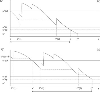
First consider the expected duration of an excursion from level u* under policy π and the expected number of accepted customers during such an excursion (i.e., Nπ(u*) and Tπ(u*)). Let the first jump, initiating an excursion, occur at time 0 and observe that the workload level right after the first jump equals u* + B (i.e., V0+π = u* + B). Note that the workload process attains local minima just before arrival instants at which customers are going to be accepted. Using terminology of random walks, define a stopping time τsπ := inf{t ≥ 0 : Vtπ ≤ u*}, an equivalent notion measured in the number of arrivals τπ := inf{k ≥ 0 : Wkπ ≤ u*}, and a sequence of descending ladder epochs τπ(1) < ··· < τπ(N) < τπ with corresponding descending ladder heights u* + B > Wτπ(1)π > ··· > Wτπ(N)π > u* as follows: τπ(1) := inf{0 ≤ k ≤ τπ : π(Wkπ) = 1}, and for n = 2,…, N (if τπ(1) < τπ),

Note that W_τ^π(N)^π > u* + δ, since π(x) = 0 for x ∈ [u*,u* + δ]. A typical sample path in case N = 2 is depicted in Figure 1a. Using the above, we write

The sample paths of two excursions of Vtπ: one excursion from state u* and one excursion from state u* + y. In this example, N = 2 and M = 3.

Now consider Nπ(u* + y) and Tπ(u* + y). In this case, at time 0 the workload jumps to u* + y + B (i.e., V0+π = u* + y + B). As defined earlier, we have a stopping time

, a discrete-time equivalent

, and a sequence of descending ladder epochs

with corresponding descending ladder heights

(see Figure 1b for a typical realization). Observe that the residual interarrival time at a downcrossing of u* + B is still exponential. Hence, using stochastic coupling and the fact that W_τ^π(N)^π > u* + δ, the descending ladder epochs can be divided into two sets: (i)

with

and (ii)

such that

for n = 1,…, N. This coupling is illustrated in Figure 1 (with N = 2 and M = 3). In this figure, the sample paths in the range of the solid arrow (i.e., between

respectively) are identical. Using the above arguments, we have

Since

, are the workloads just before an arriving customer is accepted and π is the supposed optimal policy, Lemma 3.2 yields

Moreover, using (4) and (5) in addition to Assumption 2.1, we obtain

where the second inequality relies on the fact that it is optimal to accept at level u*. Combining (6)–(9) yields

By Lemma 3.2 it cannot be strictly optimal to reject at level u* + y, 0 < y < δ. █

Theorem 3.1: There exists a threshold policy that is optimal among the class of stationary deterministic policies.

Proof: It follows from Lemma 3.3 that it is optimal to accept when the workload is in [0,z_min]. Suppose that a threshold policy is not optimal; that is, there exists some policy π that is strictly better than any threshold policy. Let

max(π(x⁺) − π(x),0) dx be the number of “gaps” of policy π (i.e., the number of times π(·) switches from zero to one). Let π be an optimal policy, which is strictly better than any threshold policy, with the least number of gaps (i.e., π = arg min_π∈Π* n^π, with Π* the class of optimal policies). This implies that there is some u* > z_min and δ₂ > δ₁ > 0 such that π(x) = 0 on (u*,u* + δ₁) and π(x) = 1 on (u* + δ₁,u* + δ₂). We note that gaps consisting of singular points can be removed.

Take some arbitrary 0 < y < δ₁. In the proof, we consider N^π(u* + y) and T^π(u* + y). Using the fact that it is optimal to accept in (u* + δ₁,u* + δ₂), we show that βN^π(u* + y)/T^π(u* + y) ≥ TH* (contradicting the fact that π contains the least number of gaps among policies in Π*). This follows from the fact that the direct reward of accepting at level u* + y exceeds the reward of accepting at any level x > u* + y. Moreover, additional excursions are only made when they are advantageous.

Suppose that at time 0 an arriving customer with service requirement B is accepted when the workload equals u* + y (i.e., V0+π = u* + y + B). As in the proof of Lemma 3.3 (see also Figure 1a, with δ1 ≡ δ), we can define “stopping times” τsπ and τπ and a sequence of descending ladder epochs τπ(1) < ··· < τπ(N) < τπ with corresponding descending ladder heights u* + y + B > Wτπ(1)π > ··· > Wτπ(N)π > u* + y. Note that Wτπ(N)π > u* + δ1 (if N > 0), since π(x) = 0 for x ∈ [u*,u* + δ1]. Applying this construction yields

By Lemma 3.2,

since π is assumed to be an optimal policy. Moreover, using a similar ladder height construction, it can be easily checked (in general) that

Hence, invoking Assumption 2.1 yields

Combining the above, we obtain βN^π(u* + y)/T^π(u* + y) ≥ TH* for any y ∈ (0,δ₁). By Lemma 3.2, this contradicts the fact that policy π has the minimum number of gaps among the class of optimal policies Π*. █

The ladder height construction in the proof of Theorem 3.1 allows us to generalize (10):

Proposition 3.1: For the throughput during an excursion from level x, we have the following bounds:

These bounds are especially natural from the perspective of the LCFS-PR discipline. In that view, the proposition simply states that the throughput during an excursion from level x is at least the minimum (and at most the maximum) of one over the mean service time of accepting at any level above x if policy π is applied.

Remark 3.1: The proof of Theorem 3.1 crucially depends on the fact that Z(·) has only one local minimum (i.e., Assumption 2.1). Suppose for the moment that Z(·) has L local minima. Thus, Z(·) is decreasing on [z_max^k,z_min^k) and increasing on [z_min^k,z_max^k+1), k = 1,…, L, where z_max¹ = 0 and z_max^L+1 = ∞. Similar to the proof of Lemma 3.3, we deduce that if π(x) = 1 for some x ∈ [z_max^k,z_min^k), then π(y) = 1 for all y ∈ [x,z_min^k) (note that π(0) = 1 and accepting is thus optimal in [0,z_min¹)). Also, it follows from the proof of Theorem 3.1 that if π(x) = 1 for some x ∈ [z_max^L,∞), then π(y) = 1 for all y ∈ [z_max^L,x). However, the intervals [z_min^k,z_max^k+1), k = 1,…, L − 1, are not covered by the proof. In particular, the trade-off between direct and future rewards remains undecided there.

Theorem 3.1 shows that the threshold policy is optimal among the class of stationary and deterministic policies. To prove that a (stationary and deterministic) threshold policy is also optimal within the broader class of policies considered in [13], we use insights from this section to construct an appropriate (value) function satisfying [13, Thm.2]. The class of policies in [13] consists of all measurable decision rules and includes nonstationary and nondeterministic policies.

Theorem 3.2: There exists a threshold policy that is optimal within the class of policies considered in [13].

Proof: Let π be a threshold policy with threshold value x* that is optimal within the class of stationary and deterministic policies. Now define n^π(x) and t^π(x) as follows:

Similar to [7], let

Consider

and divide the busy cycle in two parts; first we have an excursion from state x followed by the remaining part of the cycle starting with a downcrossing of level x. Hence (see also [7, Lemma6.3]),

where the N^π(x) − 1 stems from the fact that the arrival in state x is not counted in

.

Define, for x ≥ 0,

where x is the state of the system just before a decision epoch. By conditioning on the first arrival, we also obtain the following relationship between

:

with R⁻¹(·) the inverse function of R(·); see for example, [1,2,9] for details. Because π is assumed to be an optimal stationary deterministic policy, Lemma 3.2 yields that βN^π(x) − TH^πT^π(x) is positive for x ∈ [0,x*) and nonpositive for x ∈ [x*,∞). Using the above in addition to (11) and (12), we obtain

Combining (11) with (13), we can rewrite (14) as

Thus, the function f (·) satisfies the optimality equation for the average-cost criterion (i.e. Eq. (3) in [13]). The theorem now follows directly from [13, Thm.2]. █

4. CRITERION FOR THE OPTIMAL THRESHOLD

In Section 3 we showed that if Assumption 2.1 is satisfied, a threshold policy is optimal. The derivation of that result also suggested the following criterion for the optimal threshold:

where π_x denotes a threshold policy with parameter x. The above criterion is intuitively appealing when we consider marginal arguments. Informally speaking, the optimal threshold will be chosen such that the throughput just equals the expected reward of customers accepted in state x (which has reward β/Z(x)).

Moreover, the above criterion allows us to deduce some properties of the optimal threshold value. Using a similar construction as in (some of) the proofs of Section 3, it can be shown that TH^π_x is increasing as a function of λ. (To see this, we note that a higher λ yields additional arrivals that are only accepted if the resulting excursions are advantageous.) Because β/Z(x) is independent of λ, we can directly conclude from (15) that the optimal threshold value is decreasing in λ. It can also easily be checked that the optimal threshold approaches z_min as λ → ∞. This behavior of the optimal threshold reveals the typical trade-off between direct and future rewards; the upper bound for the throughput is attained by accepting customers in state z_min, but the optimal policy anticipates decreasing arrival rates by starting to accept customers at increasing workload levels to compensate for the increased probability of reaching an empty system (where the server is idle).

In the remainder of this section we use another method to derive a criterion for the optimal threshold value and give some properties of TH^π_x as a function of x. Moreover, when Z(·) does not satisfy Assumption 2.1, we show that a criterion similar to (15) holds for the optimal threshold value, which provides the optimal policy within the class of threshold policies. (Note that a threshold strategy might then not be optimal among the class of stationary and deterministic policies.) However, we start with the general form of the throughput under a threshold strategy with some fixed threshold x.

Observe that for fixed x, the workload under policy π_x has the same dynamics as an M/G/1 queue with a general service rate and impatience of customers depending on the amount of work found upon arrival. Under policy π_x the model is in fact a special case of the finite-buffer queue in [1], with

where

follows from normalization:

Here the (iterated) kernels are defined as in [1,9]; that is, for 0 ≤ y < x < ∞, K(x,y) := λ(1 − B(x − y))/r(x),

and

. Using the representation in (1) for the throughput, we obtain

Note that Z(x) and TH^π_x are continuous and differentiable functions of x. In order to determine the optimal threshold, it is useful to consider the derivative of TH^π_x with respect to x.

Lemma 4.1: For the derivative of TH^π_x, we have

Proof: The proof is deferred to the Appendix. █

Before we further discuss the optimal threshold criterion, we first derive some properties of TH^π_x as a function of x. As in Lemma 3.1, consider a policy π that does not accept in [a,b] and a modified policy π′, which does the same as π except that π′(x) = 1 for x ∈ [a,b]. Then the throughput under policy π′ can be written as a convex combination of the throughput under policy π and the throughput due to excursions starting from levels in [a,b] (see Lemma 3.1). This relation is particularly useful in studying the relationship between TH^π_x and Z(·).

Lemma 4.2: Suppose that (i) dZ(x)/dx ≤ 0, for x ∈ [a,b], and (ii) TH^π_a ≤ β/Z(a). Then

If either (i) (for some x ∈ [a,b]) or (ii) holds with strict inequality, then (19) holds with strict inequality. Moreover, if the (strict) inequalities in (i) and (ii) are reversed, then the (strict) inequality in (19) is reversed.

Proof: Fix an arbitrary x ∈ (a,b]. Lemma 3.1 yields that, for γ ∈ (0,1),

From (i) and Proposition 3.1, we obtain βN^π_x(y)/T^π_x(y) ≤ β/Z(x) for every y ∈ [a,x]. Invoking (ii), it trivially follows that

where the last step is due to (i). Now if (i) holds with strict inequality for some x ∈ [a,b], then the second inequality of (20) is strict, whereas the first one is strict if (ii) holds with strict inequality. The proof for the reversed signs is similar (use the lower bound in Proposition 3.1). █

We now derive a criterion for the optimal threshold. Let π_th* denote the optimal threshold strategy. Define the set A := {x ≥ 0 : TH^π_x = β/Z(x)}. Note that, in general, A is a collection of N disjoint closed intervals A_i, i = 1,…, N, where each interval can be a singleton. However, if A_i is not a singleton, then it follows directly from Lemma 4.2 that Z(·) is constant on A_i.

Proposition 4.1: If A is the empty set, then the greedy policy is optimal and TH^π_th* = r_∞. If A is nonempty,

where the greedy policy is optimal when TH^π_th* = r_∞ and the optimal (finite) threshold is given by any x ∈ arg max_x∈A β/Z(x) otherwise.

Proof: For the threshold at zero we have

If A is the empty set, then we have from the continuity of Z(·) and TH^π_x that TH^π_x < β/Z(x) for all x. Applying Lemma 4.1, we obtain that d(TH^π_x)/dx > 0 for all x and the greedy policy is thus optimal.

If N > 0, then it follows from Lemma 4.1 that A contains all points satisfying dTH^π_x/dx = 0. Hence, A contains at least all extreme points. From (21) and Lemma 4.1 it follows that zero is a local minimum. Moreover, TH^π_x → r_∞ as x → ∞. Because TH^π_x is continuous, finding the global maximum of TH^π_x reduces to finding the maximum of β/Z(x), x ∈ A, and comparing it with r_∞. █

Using Lemma 4.2, some additional properties of TH^π_x as a function of x can be derived. For instance, it can be shown that if Z(·) has m local maxima, then N ≤ 2m − 1. In particular, if Assumption 2.1 is satisfied, then N ≤ 1. This case is of special interest because a threshold policy is then optimal. Moreover, if in that case N = 1, then A ∩ [0,z_min) is empty and each value in A (possibly a singleton) is a global maximum of TH^π_x. These arguments are summarized in the following corollary.

Corollary 4.1: Suppose that Assumption 2.1 is satisfied. If A is the empty set, then the greedy policy is optimal. Otherwise, N = 1 and x ∈ A is an optimal threshold with corresponding throughput

Finally, if r(x) is constant for x ≥ L (and Assumption 2.1 holds), there is an easy way to determine directly whether the greedy policy is optimal. From Lemma 4.2 we then deduce the following:

Corollary 4.2: Suppose Assumption 2.1 is satisfied and r(x) = r_∞ for all x ≥ L for some L > 0. Then the greedy policy is optimal if and only if

5. ASSUMPTION ON Z(x)

Although Assumption 2.1 is quite natural, it involves the service-rate function as well as the distribution of the service requirement. In this section we give some examples satisfying this assumption, assuming that r(·) is increasing on (0,r_max] and decreasing on (r_max,∞) for some r_max ≥ 0 (as described in Section 2). We consider both cases with general service requirement distributions and cases with a wide class of service-rate functions. In addition, we provide a natural example that does not have the desired properties. This case reveals the strong dependence on both the service-rate function and the service requirement distribution.

To show that Assumption 2.1 is satisfied, we frequently use the derivative of Z(·). Interchanging derivative and sum in addition to some rewriting yields

For Assumption 2.1 to be satisfied, it remains to be shown that

Example 5.1: Suppose that r_max = 0 (i.e., r(·) is decreasing on the positive half-line). By definition, r(y) ≥ r(x) for y > x, and it is readily seen that Assumption 2.1 is satisfied. Also, z_min = 0 in this case.

Example 5.2: Suppose that B(x) = I(x ≥ β) (i.e., the service requirement is deterministic β). Observe that

is just the shifted r(·) function. Thus,

if x ∈ [0,(r_max − β)⁺] and

if x ∈ [r_max,∞). Moreover, r(x) is increasing on [(r_max − β)⁺,r_max], whereas

is decreasing on the same interval. This directly yields the required property.

Example 5.3: Suppose that B(x) = 1 − e^−μx, meaning that the service requirement is exponentially distributed. Observe that

for x ≥ r_max. Now take some arbitrary x and y, with 0 < x < y ≤ r_max. Conditioning on the service requirement in case a customer arrives at level x and using the memoryless property of the exponential distribution, we have

and, thus,

Note that if

, then

(since r(y) ≥ r(x)). Similarly, if

, then

. This directly gives the desired property, where

.

Example 5.4: Suppose that r(·) is defined as follows:

In addition, assume that r_∞ ≥ r₁. From the properties of r(·), it is obvious that

. Hence, a ≤ z_min ≤ r_max. Now take arbitrary x,y, with a ≤ x < y ≤ r_max. First consider the following:

where we used that r(·) is concave on [a,r_max] and decreasing on [r_max,∞) in the second step. Using the above, we obtain

As in Example 5.3, note that if

, then

(since r(y) ≥ r(x)). Similarly, if

, then

. Hence, Assumption 2.1 is satisfied, with

.

Finally, note that Example 5.1 is just a special case (take a = r_max = 0). However, we believe that Example 5.1 is a natural special case, which admits an easy verification of Assumption 2.1.

Example 5.5: Here we provide an example for which Assumption 2.1 is not satisfied. For simplicity, we choose specific values for some model parameters. A slightly more general model could be constructed by leaving some parameters unspecified while leaving the structure unaltered.

Consider the following service rate function:

with

, implying that

. Also, suppose that B = a/3 with probability

with probability ½, and take c > 3(r₁ − r₂)/a. After some calculations, we derive that dZ(x)/dx is strictly positive on (0,a/3) and ((2a/3) + (r₁ − r₂)/c,(4a/3) − (r₁ − r₂)/c) and strictly negative on (a/3,(2a/3) + (r₁ − r₂)/c) and ((4a/3) − (r₁ − r₂)/c,∞). Clearly, Z(·) has two local minima and Assumption 2.1 is not satisfied in this case.

6. SOME EXAMPLES

In general, (18) is suitable for a numerical calculation of the optimal threshold. Also, the characteristics of TH^π_x described in Section 4 suggest another numerical calculation of this optimal value, for instance, using a bisection method. In this section we give some examples in which we obtain an analytically more tractable expression for the optimal throughput with the corresponding optimal threshold value. In Section 6.1 we consider a two-level service rate: The service rate at time t is r₁ when V_t^π ≤ a and r₂ < r₁ when V_t^π ≥ a (see, for instance, [5]). In Section 6.2, we generalize the service rate to an arbitrary step function, but we restrict ourselves to exponential service requirements there.

In any case, if the greedy policy is not optimal, the optimal threshold value must satisfy (15); see Proposition 4.1. Define

where

represents a nonnormalized workload distribution. Using (18) and some straightforward manipulations, we can rewrite (15) as

Note that both

and finite. Thus, finding the extremes of TH^π_x reduces to solving z(x) = 0.

6.1. Two-Level Service Rate

Suppose that the service rate is specified as

where 0 < r₂ < r₁. Define ρ_i := λβ/r_i, i = 1,2. Because the service-rate function is decreasing, we obtain from Example 5.1 that Assumption 2.1 is satisfied and a threshold policy is thus optimal. To determine the optimal threshold x, we derive from Corollary 4.2 that we only need to consider x ≤ a.

Fix some x ∈ [0,a]. Using results of [1,9], the stationary workload distribution can be easily reduced to a more tractable expression. Let

be the stationary residual service requirement distribution with density h(·). For x ≤ a, K(x,y) = ρ₁ h(x − y) and it is well known that

, where h_n(·) is the density of the n-fold convolution H_n(·) (see, e.g., [1,9]).

Now we determine the three elements on the right-hand side of (22) separately, after which we combine them to determine z(x). First consider λZ(x). Using the definitions of Z(·) and H(·), respectively (2) and (23), yields

Second, consider the nonnormalized workload distribution W(·). Interchanging integral and sum in addition to the above results, we immediately obtain for each x ∈ [0,x],

Remark 6.1: Note that W(·)/W(a) is the steady-state workload distribution in a finite dam with speed r₁ and buffer size a. In the case ρ₁ < 1, it is an easy exercise to see that the Laplace–Stieltjes transform of W(·) provides the well-known Pollaczek–Khinchine formula. If

is still finite and a steady-state workload distribution exists (see, e.g., [9]). However, Cohen [4,5] describes a more elegant way to determine W(·) in that case.

Finally, the first term of (22) (i.e., the inverse of the normalizing constant

), is the most complicated one. Using the expression for the steady-state workload density in addition to the above results, we derive for x < x ≤ a,

where we used W(0) = 1 in the final step. Note that for x > a, K(x,y) = ρ₂ h(x − y). Using similar arguments, we obtain for x > a,

By (25), we have

. Letting x → ∞ and some rewriting then yields

It is now easy to get z(x). Substituting (24)–(26) into (22) gives

Summarizing, Corollary 4.2 implies that the greedy policy is optimal if and only if

Otherwise, TH* = ρ/(ρ₂ + (ρ₁ − ρ₂)H(a − x*)), with ρ := λβ and x* is a solution to z(x*) = 0.

In general, the convolution in (27) can only be determined numerically. However, if the service requirement follows a phase-type distribution, explicit expressions can be obtained. For instance, if B(x) = 1 − e^−μx (see also Section 6.2), then after quite lengthy but standard calculations, it follows that for ρ₁ ≠ 1,

In the case ρ₁ = 1, we obtain

6.2. Exponential Service Requirements

Suppose that the service requirements are exponentially distributed with mean 1/μ (i.e., 1 − B(x) = e^−μx). Then, for fixed x, the steady-state workload density is given in [1, Cor. 7.1]

where

follows from normalization. In this subsection, we also assume that the service rate is a step function. More specifically, let r(x) = r_i for x ∈ [a_i−1,a_i), i = 1,…, N (where a₀ = 0), and let r(x) = r_N+1 < r_N for x ≥ a_N. Denote ρ_i = λ/(μr_i), i = 1,…, N + 1, and assume for simplicity that ρ_i ≠ 1.

Example 5.3 shows that Assumption 2.1 is satisfied and a threshold policy is thus optimal. By Corollary 4.2, either the greedy policy is optimal or the optimal threshold x* is less than a_N. Let x ∈ [a_n,a_n+1) for some n ≤ N − 1. Next we consider each of the three elements of z(x) separately, after which we combine them into an expression for x* satisfying (15). However, for later use, we first define the following three constants. (In the sequel, we follow the convention that empty sums are equal to zero.):

First, consider λZ(x). Using (2) and rewriting the integral, we obtain

Second, consider W(·) (i.e., the workload distribution “without normalization”). It is easily checked that the time to empty the system starting from a_i, i = 1,…, n, in the absence of any arrivals (i.e., R(a_i)) equals

. Hence, for x ∈ [a_i,a_i+1), we can deduce that

Now, for i = 1,…, n, using (29) and (31), after some standard algebra we obtain that

where we used γ_k e^{μρ_k+1 a_k} = γ_k−1 e^{μρ_k a_k} in the fourth equality. Thus, combining (29) and (31) with the above, we obtain, after similar manipulations,

which completes the calculation of W(·) (since

).

For the first term on the right-hand side of (22) (i.e.,

), we use similar arguments as for the previous term. We first consider V^π_x(x) with x > a_n+1 and let i = arg max{a_i : a_i ≤ x} be the largest a_i smaller than x. Using (29) and applying (31) to determine λR(x), we obtain after algebra similar to that above, that

Thus, letting x → ∞, we obtain the normalizing constant:

The function z(x) can now easily be rewritten into a more appealing expression. In particular, substituting (30), (34), and W(x) resulting from (33) into (22) and some reordering of terms yields

Solving z(x) = 0 is thus remarkably simple in this case, since the variable x only appears in two of the exponents. Summarizing, we conclude that the optimal policy is of the threshold type where the optimal threshold value is given by the solution of z(x) = 0. Moreover, TH* = β/Z(x), where λZ(x) is given in (30).

Remark 6.2: It is easily checked that, in case N = 1, the formula for z(x) indeed reduces to (28).

7. CONCLUDING REMARKS AND FURTHER RESEARCH

In the present article we considered the problem of optimal admission control in a system with a workload-dependent service rate. We assumed that the service requirement only becomes known right after the decision to accept or reject jobs. Our objective was to find a policy that maximizes the long-run throughput. Under some assumptions (in particular, Assumption 2.1), we showed that a threshold policy for accepting jobs is optimal and derived a criterion for the optimal threshold value.

We note that our main assumption (i.e., Assumption 2.1) involves sufficient conditions for optimality of threshold policies. An interesting subject for further research is to examine the structure of the optimal policy when Assumption 2.1 is not satisfied.

Moreover, there are various interesting model variations. For instance, the analysis is significantly changed if information about the service requirement is available. In that case, the decision will not only depend on the workload level but also on the size of the job, yielding a two-dimensional state space. A characterization of the optimal policy in that model might be a subject of further study. We note that a threshold policy will not be optimal in general. However, in some special cases, such as for deterministic service requirements or decreasing service rate functions, the optimal policy continues to be of the threshold type.

Other model variations are systems where jobs can be partly accepted (or rejected). The simplest version concerns a model where an infinite amount of work becomes available at Poisson instants and the policy prescribes the amount of work to accept. In some sense, this model is related to the case λ → ∞ in the model of the present article, which might be interpreted as an infinite supply of jobs and the policy prescribes the time to accept a new job. More interesting are systems where the supply of work is bounded by the service requirements of arriving jobs and the decision is the amount of work to accept. In that case, the state space is two dimensional and the action space is continuous. The structure of the optimal policy in the latter model is also left for future investigation.