1. Introduction
Magnetohydrodynamic (MHD) turbulence has been the focus of extensive research due to its profound relevance across various domains, spanning natural phenomena such as geophysics and astrophysics, as well as engineering applications like plasma confinement, liquid metal cooling in nuclear reactors, electromagnetic casting and beyond. In this study, large-eddy simulations (LES) are employed to investigate the flow of an electrically conducting, incompressible fluid within a periodic box under the influence of an external magnetic field. It is assumed that the magnetic Reynolds number (
 $Re_m$
) is much smaller than unity, signifying that the magnetic field
 $\boldsymbol{b}$
generated by electric currents in the liquid metal is negligible compared with the externally applied magnetic field
 $\boldsymbol{B}$
. The Lorentz force acting on the flow, described by
 ${\boldsymbol{F}}_{Lorentz} = {\boldsymbol{j}} \times {\boldsymbol{B}}$
under the quasistatic approximation (Roberts Reference Roberts1967), where
 $\boldsymbol{j}$
denotes the electric current density, primarily elongates flow structures along the direction of the magnetic field, thereby inducing strong anisotropic characteristics in the turbulence (Sommeria & Moreau Reference Sommeria and Moreau1982; Zikanov & Thess Reference Zikanov and Thess1998; Vorobev et al. Reference Vorobev, Zikanov, Davidson and Knaepen2005; Krasnov, Zikanov & Boeck Reference Krasnov, Zikanov and Boeck2012; Reddy, Kumar & Verma Reference Reddy, Kumar and Verma2014; Zikanov et al. Reference Zikanov, Krasnov, Boeck and Sukoriansky2019; Chen et al. Reference Chen, Pothérat, Ni and Moreau2021). In decaying MHD turbulence, this evolution is typically categorised into two distinct stages: a linear stage and a nonlinear stage (Moffatt Reference Moffatt1967; Davidson Reference Davidson1995; Sreenivasan & Alboussière Reference Sreenivasan and Alboussière2000; Sreenivasan & Alboussiere Reference Sreenivasan and Alboussiere2002; Wang et al. Reference Wang, Chen, Cao, Ke, Yang and Ni2023).
The theoretical investigation by Moffatt (Reference Moffatt1967) marks a significant milestone in the modern understanding of the decay of quasistatic MHD turbulence. In particular, Moffatt (Reference Moffatt1967) proposed a linear hypothesis that, for
 $N \gg 1$
and
 $\tau \ll t \ll T$
(where
 $\tau$
denotes the magnetic damping time and
 $T$
is the eddy turnover time), turbulent energy decays following a scaling law of
 $K \sim (t/\tau )^{-1/2}$
. Furthermore, he suggested that at the end of the linear stage, the kinetic energy component
 $K_{\parallel }$
parallel to
 $\boldsymbol{B}$
should be twice that of the vertical component
 $K_{\bot }$
, a prediction that has been verified by numerous numerical simulations (Schumann Reference Schumann1976; Favier et al. Reference Favier, Godeferd, Cambon and Delache2010; Burattini, Zikanov & Knaepen Reference Burattini, Zikanov and Knaepen2010). The initial experimental study of MHD turbulence in a duct was conducted by Kolesnikov & Tsinober (Reference Kolesnikov and Tsinober1974), who observed that the magnetic field reduced the decay rate of kinetic energy. In contrast, Alemany et al. (Reference Alemany, Moreau, Sulem and Frisch1979), in a subsequent experiment on grid turbulence, found the opposite: the magnetic field increased the decay rate of kinetic energy. While these two findings seem contradictory, the difference is likely attributable to the distinct experimental set-ups: the duct flow studied by Kolesnikov & Tsinober (Reference Kolesnikov and Tsinober1974) was confined and geometrically constrained, whereas the grid turbulence experiment by Alemany et al. (Reference Alemany, Moreau, Sulem and Frisch1979) was in a more homogeneous, unbounded configuration. Furthermore, to differentiate the modes that have already lost part of their energy due to Joule dissipation from those which contain mostly the kinetic energy in Fourier space, Moreau (Reference Moreau1990) introduced the definition of the Joule cone (as illustrated in figure 1
a) and hypothesised that the Joule cone angle
 $\theta$
as half of the Joule cone, follows
 $\cos \theta \sim t^{-1/2}$
. Alemany et al. (Reference Alemany, Moreau, Sulem and Frisch1979) also predicted the existence of a quasiequilibrium state between angular energy transfer and Joule dissipation, which was supported by one-dimensional energy spectral measurements showing a spectral slope of
 $\Phi _{\parallel }(k) \sim k_{\parallel }^{-3}$
, where
 $\Phi _{\parallel }$
represents the spectral tensor component parallel to the magnetic field. However, this quasiequilibrium state has been challenged by several studies (Knaepen, Kassinos & Carati Reference Knaepen, Kassinos and Carati2004; Vorobev et al. Reference Vorobev, Zikanov, Davidson and Knaepen2005; Burattini et al. Reference Burattini, Zikanov and Knaepen2010; Favier et al. Reference Favier, Godeferd, Cambon and Delache2010), which found that viscous dissipation becomes equal to Joule dissipation in the late stages of the decay process.
Sketches of (a) the Joule cone in Fourier space, (b)
 $\psi _t$
in Fourier space at time
 $t$
. Here
 $k_{\parallel }$
and
 $k_{\bot }$
represent the coordinates parallel and perpendicular to the magnetic field in Fourier space, respectively. In (a)
 $\theta$
, referred to as the Joule cone angle (as defined in (3.3)) denotes the angle between the edge of Joule cone and the
 $k_{\parallel }-$
axis. In (b),
 $\psi _t$
satisfies
 $\tau _t(\psi _t)=t$
(where
 $\tau _t$
is defined in (3.11)). For
 $\psi \langle \psi _t$
,
 $\eta \rangle 1$
(with
 $\eta$
defined as
 $ \sqrt {2}\cos \psi ( {t}/{\tau } )^{1/2}$
).

Another theoretical framework for the free decay of homogeneous MHD turbulence was established by Davidson (Reference Davidson1997), who studied a flow in a sphere domain and concluded that when
 $N \gg 1$
, the flow ultimately evolves towards a two-dimensional state due to the conservation of the global angular momentum component parallel to the magnetic field. Concurrently, the integral length scale along the magnetic field,
 $l_z$
, increases as
 $l_z \sim t^{1/2}$
. Sreenivasan & Alboussiere (Reference Sreenivasan and Alboussiere2002) generated a single vortex using electric currents and magnetic fields, and through the evolution of turbulent kinetic energy during the decay process, provided indirect evidence supporting the theory of Davidson (Reference Davidson1995). Furthermore, Davidson (Reference Davidson2001) proposed that viscous dissipation and Joule dissipation are, respectively, proportional to
 $u'^3/l_{\bot }$
and
 $u'^2l_{\parallel }l_{\bot }^{4}/\tau$
, where
 $l_{\bot }$
and
 $l_{\parallel }$
represent the characteristic length scales perpendicular and parallel to the magnetic field, a theory later confirmed by Okamoto, Davidson & Kaneda (Reference Okamoto, Davidson and Kaneda2010) using the invariance of the ‘parallel’ component of Loitsyansky’s integral
 $I_{\parallel }$
. Subsequently, Wang et al. (Reference Wang, Chen, Cao, Ke, Yang and Ni2023) conducted a numerical investigation of the decay of a single vortex under a magnetic field. By probing the angular momentum, he confirmed the validity of the theory of Davidson (Reference Davidson1995) and also identified the discrepancy between global energy evolution and local energy evolution.
In recent years, MHD turbulence has played a pivotal role in the study of turbulence energy transfer (Favier et al. Reference Favier, Godeferd, Cambon and Delache2010; Klein & Pothérat Reference Klein and Pothérat2010; Pothérat & Klein Reference Pothérat and Klein2014; Baker, Pothérat & Davoust Reference Baker, Pothérat and Davoust2015; Pothérat & Kornet Reference Pothérat and Kornet2015; Baker et al. Reference Baker, Pothérat, Davoust and Debray2018; Chen et al. Reference Chen, Pothérat, Ni and Moreau2021). Reddy & Verma (Reference Reddy and Verma2014) numerically observed the existence of bidirectional energy cascade in forced MHD turbulence. Furthermore, Reddy et al. (Reference Reddy, Kumar and Verma2014) found that the velocity component parallel to the magnetic field controls direct energy cascade, while the velocity component perpendicular to the magnetic field governs inverse energy cascade. Subsequently, Baker et al. (Reference Baker, Pothérat, Davoust and Debray2018) experimentally observed bidirectional energy cascade in MHD turbulence through the FlowCube experimental platform (Klein & Pothérat Reference Klein and Pothérat2010; Pothérat & Klein Reference Pothérat and Klein2014) and highlighted the significant impact of dissipation methods on energy transport. However, the energy transport in decaying MHD turbulence remains unexplored, raising questions about the potential existence of bidirectional transport in this context.
These discoveries inspire us to perform numerical simulations of decaying MHD turbulence. In this work, we aim to address the following overarching questions.
-
(i) Does a scaling law of
 $t^{-1/2}$
for the Joule cone exist, as proposed by Moreau (Reference Moreau1990)? How does the Joule cone evolve throughout the decay process, and how does this evolution manifest across different wavenumbers?
-
(ii) According to the linear assumption proposed by Moffatt (Reference Moffatt1967), does the scaling law of
$K\sim t^{-1/2}$
hold precisely, or do new phenomena arise when the interaction number becomes sufficiently large? -
(iii) Is there a quasiequilibrium state between angular energy transfer and Joule dissipation that leads to a scaling law of
$E(k) \sim k^{-3}$
in the inertial subrange? -
(iv) What is the nature of energy transfer between velocity components? Does a bidirectional transfer exist in decaying MHD turbulence, as observed by Baker et al. (Reference Baker, Pothérat, Davoust and Debray2018)? If so, how does this bidirectional energy transfer evolve during the decay process?


The paper is organised as follows. In § 2, a short description of the physical model underlying this work and the flow conditions is given. The numerical algorithm and case set-up are also presented in this part. The main properties of the free decaying MHD turbulence are described and discussed in § 3, including decay laws of the linear stage, kinetic energy spectrum and energy transfer. Finally, we offer concluding remarks in § 4.
2. Problem statement and formulation
2.1. Governing equations and numerical method
The flow of an incompressible, electrically conducting fluid in a periodic box subjected to an external magnetic field aligned along the
 $z$
axis is considered. Assuming the asymptotic limit of low magnetic Reynolds and Prandtl numbers, the Navier–Stokes equations for an incompressible fluid can be approximated to the first order, as follows (Roberts Reference Roberts1967):
 \begin{align} \nabla \cdot {\boldsymbol{u}} =0 , \\[-27pt] \nonumber \end{align}
 \begin{align} \frac {\partial {\boldsymbol{u}}}{\partial t}+({\boldsymbol{u}}\cdot \nabla ){\boldsymbol{u}}=-\frac {1}{\rho }\nabla p+\nu \Delta {\boldsymbol{u}}+\frac {{\boldsymbol{j}}\times {\boldsymbol{B}}}{\rho }, \\[-27pt] \nonumber \end{align}
 \begin{align} {\boldsymbol{j}}=\sigma (-\nabla \varphi +{\boldsymbol{u}}\times {\boldsymbol{B}}), \\[-27pt] \nonumber \end{align}
 \begin{align} \nabla \cdot {\boldsymbol{j}} =0 , \\[-27pt] \nonumber\end{align}
 \begin{align} \nabla ^2 \varphi = \nabla \cdot ({\boldsymbol{u}}\times {\boldsymbol{B}}) . \\[6pt] \nonumber \end{align}
Here, the variables
 $\boldsymbol{j}$
,
 $\varphi$
,
 $\boldsymbol{u}$
,
 $p$
,
 $\nu$
,
 $\sigma$
and
 $\rho$
represent the current density, electric potential, velocity, pressure, kinematic viscosity, electrical conductivity and fluid density, respectively. The numerical simulations of the governing equations are performed using the finite volume method with LES. The Poisson equation for the electric potential is solved using a consistent and conservative scheme (Ni et al. Reference Ni, Munipalli, Huang, Morley and Abdou2007). Detailed descriptions and verification of this approach can be found in Chen et al. (Reference Chen, Pothérat, Ni and Moreau2021). In this study, the dynamic Smagorinsky model (DSM) (Germano et al. Reference Germano, Piomelli, Moin and Cabot1991; Lilly Reference Lilly1992) is employed, a model that has been shown to be highly accurate for MHD turbulence, as verified by Knaepen & Moin (Reference Knaepen and Moin2004), Vorobev et al. (Reference Vorobev, Zikanov, Davidson and Knaepen2005) and Burattini et al. (Reference Burattini, Zikanov and Knaepen2010).
2.2. Dynamic subgrid model
In LES, the flow is resolved only at large and moderate length scales. By applying a spatial filtering to the governing equations (2.1–2.5), the resulting equations describe the filtered fields, indicated by an overbar,
 \begin{align} \nabla \cdot \bar {{\boldsymbol{u}}} =0 , \\[-27pt] \nonumber \end{align}
 \begin{align} \frac {\partial \bar {{\boldsymbol{u}}}}{\partial t}+(\bar {{\boldsymbol{u}}}\cdot \nabla )\bar {{\boldsymbol{u}}}=-\frac {1}{\rho }\nabla \bar {p}+\nu \Delta \bar {{\boldsymbol{u}}}-\nabla \cdot \tau _{\textit{sgs}}^a+ \frac {\bar {{\boldsymbol{\kern-1.5pt j}}}\times {\boldsymbol{B}}}{\rho } , \\[-27pt] \nonumber \end{align}
 \begin{align} \bar {{\boldsymbol{\kern-1.5pt j}}}=\sigma (-\nabla \bar {\varphi }+\bar {{\boldsymbol{u}}}\times {\boldsymbol{B}}) , \\[-27pt] \nonumber \end{align}
 \begin{align} \nabla \cdot \bar { {\boldsymbol{\kern-1.5pt j}}} =0 , \\[-27pt] \nonumber \end{align}
 \begin{align} \nabla ^2\bar { \varphi } = \nabla \cdot (\bar {{\boldsymbol{u}}}\times {\boldsymbol{B}}) , \\[-6pt] \nonumber \end{align}
where
 $\tau _{\textit{sgs}}^{a}$
is the traceless subgrid-scale stress tensor and is defined with subgrid-scale stress tensor
 $\tau _{ij}$
by
 \begin{equation} \tau _{\textit{sgs}}^{a}=\tau _{ij}-\frac {1}{3} \tau _{aa}\delta _{ij}, \quad \tau _{ij}=\overline {u_{i}u_{j}}-\bar {u_{i}}\bar {u_{j}} .\end{equation}
To close the filtered equations, the tensor
 $\tau _{ij}$
needs to be modelled in terms of the resolved fields. In this study, the DSM is employed, which relies on the eddy-viscosity hypothesis and assumes that
 \begin{equation} \tau _{ij}=-2\nu _t\bar {S}_{ij}=-2C_{D}(\bar {\unicode{x1D6E5} })^{2}|\bar {S}|\bar {S}_{ij} ,\end{equation}
where
 $\nu _t$
is the turbulent viscosity and
 $C_D$
is the dynamic Smagorinsky constant. The velocity
 $-$
strain tensor for the resolved component
 $\bar {S}_{ij}$
and its magnitude
 $|\bar {S}|$
are defined by
 \begin{equation} \bar {S}_{ij}=\frac {1}{2}\left (\frac {\partial {\bar {u}_{i}}}{\partial {x_{j}}}+\frac {\partial {\bar {u}_{j}}}{\partial {x_{i}}}\right ), \quad |\bar {S}|=\sqrt {2\bar {S}_{ij}\bar {S}_{ij}} .\end{equation}
Germano et al. (Reference Germano, Piomelli, Moin and Cabot1991) proposed the so-called dynamic procedure, later optimised with a least-square method suggested by Lilly (Reference Lilly1992). In this dynamic procedure, the model parameter
 $C_D$
of the DSM is determined by averaging along the homogeneous directions as
 \begin{equation} C_{D}=\frac {\langle L_{ij}M_{ij}\rangle }{M_{ij}M_{ij}} ,\end{equation}
where
 $L_{ij}$
and
 $M_{ij}$
are defined as
 \begin{align}&\qquad L_{ij}=\widetilde {\bar {u_{i}}\bar {u_{j}}}-\tilde {\bar {u_{i}}}\tilde {\bar {u_{j}}} ,\end{align}
 \begin{align}& M_{ij}=2\bar {\unicode{x1D6E5} ^2}\widetilde {|\bar {S}_{ij}|\bar {S}_{ij}}-2\tilde {\bar {\unicode{x1D6E5} }}^2\tilde {\bar {|S|}}\tilde {\bar {S}}_{ij} ,\end{align}
where the test filter
 $\tilde {\bar {\unicode{x1D6E5} }}$
is given by
 \begin{equation} \frac {\tilde {\bar {\unicode{x1D6E5} }}}{\bar {\unicode{x1D6E5} }}=2 .\end{equation}
Knaepen & Moin (Reference Knaepen and Moin2004) used the pseudospectral method to demonstrate that dynamic LES can be applied to MHD turbulence. Building on this, we use DNS with the finite volume method to validate that dynamic LES can accurately capture the pole–equator anisotropy in MHD turbulence. The detailed verification process is provided in Appendix A.
2.3. Theoretical fundamentation
Since the mean velocity and shear are assumed to be zero, the evolution of the Reynolds stress tensor is obtained by multiplying by
 $u_{j}$
, performing space averaging and symmetrizing:
 \begin{equation} \frac {\mathrm{d} \langle \bar {u}_i\bar {u}_j\rangle }{\mathrm{d} t}=-\underbrace {\frac {1}{\rho }\left \langle \bar {p} \left (\frac {\partial \bar {u}_i}{\partial x_j}+\frac {\partial \bar {u}_j}{\partial x_i} \right ) \right \rangle }_{P_{ij}} - \underbrace {2 (\nu +\nu _t)\left \langle \frac {\partial \bar {u}_i}{\partial x_k}\frac {\partial \bar {u}_j}{\partial x_k} \right \rangle }_{\epsilon _{ij}} - \underbrace {\left \langle 2\frac {j_i j_j}{\sigma }\right \rangle }_{\epsilon _{J_{ij}}} .\end{equation}
Here, summation is implied over the same index, and for simplicity, the overbar representing the resolved field is omitted hereafter. Here
 $\langle .\rangle$
denotes the space averaging over homogeneous directions. The three tensors
 $P_{ij}, \epsilon _{\nu _{ij}}$
and
 $\epsilon _{J_{ij}}$
represent the effects of the pressure-rate-of-strain correlation, viscous dissipation and Joule dissipation. The trace of equation (2.18) yields an equation for the turbulent kinetic energy
 \begin{equation} \frac {\mathrm{d}}{\mathrm{d} t} \underbrace {\left \langle \frac {1}{2} u_iu_i \right \rangle }_{K}= - \underbrace {2 (\nu +\nu _t)\left \langle \frac {\partial u_i}{\partial x_k}\frac {\partial u_i }{\partial x_k} \right \rangle }_{\epsilon _{\nu }} - \underbrace {\left \langle 2\frac {j_i j_i}{\sigma }\right \rangle }_{\epsilon _{J}} .\end{equation}
In Fourier space, the spectral tensor (Pope Reference Pope2001) can be expressed as follows:
 \begin{equation} \frac {\partial \Phi _{ij}({\boldsymbol{k}})}{\partial t}=\Pi _{p,ij}({\boldsymbol{k}})+T_{ij}({\boldsymbol{k}})-2(\nu +\nu _t) k^2 \Phi _{ij}({\boldsymbol{k}})-\frac {\sigma B^2}{\rho } \cos ^2 \psi \Phi _{ij}({\boldsymbol{k}}) .\end{equation}
Here,
 $\Phi _{ij}$
represents the product of
 $\hat {u}_{i}(\textbf {k})$
and
 $ \hat {u}_{j}^{*}({\boldsymbol{k}})$
, where
 $\hat {.}$
denotes the Fourier transform, the asterisk signifies the complex conjugate (in this context) and
 $\boldsymbol{k}$
represents the wavenumber vector in Fourier space. Here
 $\nu _t$
represents the turbulent viscosity. Here
 $\Pi _{p,ij}({\boldsymbol{k}})$
and
 $T_{ij}({\boldsymbol{k}})$
are the Fourier transforms of the pressure-rate-of-strain correlation tensor (referred to as the pressure term) and the nonlinear transfer tensor, respectively. Here
 $\psi$
denotes the angle between the wavenumber vector
 $\boldsymbol{k}$
and the magnetic field in the spherical coordinate system
 $(k, \phi , \psi )$
.
The formula for calculating the three-dimensional energy spectrum is given by (2.21). For isotropic turbulence, the three-dimensional spectrum is derived from the shell average of
 $\Phi _{ij}({\boldsymbol{k}})$
. However, in the case of MHD turbulence, strong anisotropy induced by Joule dissipation causes
 $\Phi _{ij}({\boldsymbol{k}})$
depend on
 $\psi$
. Thus, it is more appropriate to use a ring average and integrate over the shell to compute the three-dimensional energy spectrum in spectral space (Favier et al. Reference Favier, Godeferd, Cambon and Delache2010; Reddy et al. Reference Reddy, Kumar and Verma2014; Verma Reference Verma2017),
 \begin{equation} E(k)=k^2\int _0^{2\pi } \int _{-1}^{1} \Phi _{ii}({\boldsymbol{k}}) \mathrm{d}\cos \psi \mathrm{d}\phi .\end{equation}
The turbulent energy in spectral space is calculated as
 $K=\int _{0}^{\infty } E(k){\rm d}k$
(Davidson Reference Davidson2015). The control parameters for decaying MHD turbulence are the Reynolds number
 $Re_l=(2K/3)^{1/2}l/\nu$
and the interaction number
 $N=\sigma B^2 l/\rho (2K/3)^{1/2}$
, where
 $l$
is the integral length, determined from the initial isotropic field as follows:
 \begin{equation} l= \frac {3\pi \int _{0}^{\infty }E(k)/k {\rm d}k}{4K} .\end{equation}
In homogeneous anisotropic turbulence, the one-dimensional integral length scale (Pope Reference Pope2001) is defined as
 \begin{equation} l_i=\frac {\pi \phi _{ii}(0)}{\langle {u}_i^2\rangle } ,\end{equation}
where
 $\phi _{ii}$
is the one
 $-$
dimensional energy spectrum (Pope Reference Pope2001). In homogeneous isotropic turbulence,
 $l \equiv l_{i}$
. Sreenivasan & Alboussière (Reference Sreenivasan and Alboussière2000) proposed a revised interaction number
 $N_{t}$
to more accurately reflect the ratio of the Lorentz force to inertia
 \begin{equation} N_{t}=N\left( \frac {l_{\bot }}{l_{\parallel }}\right)^2 ,\end{equation}
where
 $l_{\parallel }$
,
 $l_{\bot }$
are the integral length scales parallel and perpendicular to the magnetic field, respectively. In our simulations, the initial turbulent energy spectrum is given by
 \begin{equation} E(k,0)=k^{-5/3}\left [\frac {kL}{[(kL)^4+C_{L}]^{1/4}}\right ]^{5/3 + p_0} ,\end{equation}
where
 $p_0$
denotes the slope at low
 $k$
, the exponent
 $-5/3$
elucidates the inertial subrange. The precise definition of
 $C_L$
is provided in Burattini et al. (Reference Burattini, Zikanov and Knaepen2010). Notably, the initial conditions in our simulations are fully consistent with those outlined in Burattini et al. (Reference Burattini, Zikanov and Knaepen2010).
Owing to the preferential elongation of turbulent structures along the
 $\boldsymbol{B}$
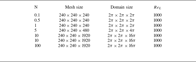
direction, the numerical domain is extended in this direction, allowing for longer simulations before the assumption of periodic boundaries becomes questionable. Our study models seven cases with the interaction number ranging from
 $0.1$
to
 $100$
. The grid resolution and domain size are presented in table 1, and in all simulations, the integral length
 $l_i$
remains less than
 $L_i/8$
to ensure the validity of the periodic boundary condition (Wang & George Reference Wang and George2002).
Cases set-up.

2.4. Energy transfer in Fourier space
The investigation of energy transfers in Fourier space can be conducted in detail through the ‘mode-to-mode’ energy transfer framework introduced by Domaradzki & Rogallo (Reference Domaradzki and Rogallo1990), Dar, Verma & Eswaran (Reference Dar, Verma and Eswaran2001) and Teaca et al. (Reference Teaca, Verma, Knaepen and Carati2009); Reddy et al. (Reference Reddy, Kumar and Verma2014). For a triad
 $({\boldsymbol{k}}, {\boldsymbol{p}}, {\boldsymbol{q}})$
, the energy transfer rate between modes is given by
 \begin{equation} S({\boldsymbol{k}} \mid {\boldsymbol{p}} \mid {\boldsymbol{q}}) = \textrm{Im} \big \{ [{\boldsymbol{k}} \cdot \widehat {{\boldsymbol{u}}}({\boldsymbol{q}})] \big [ \widehat {{\boldsymbol{u}}}^*({\boldsymbol{k}}) \cdot \widehat {{\boldsymbol{u}}}({\boldsymbol{p}}) \big ] \big \} \end{equation}
where
 $\textrm{Im}$
represents the imaginary part and the asterisk denotes the complex conjugate. This quantity describes the energy transfer from mode
 $\boldsymbol{p}$
to mode
 $\boldsymbol{k}$
, with mode
 $\boldsymbol{q}$
acting as a mediator. It is essential to note that the relationship
 ${\boldsymbol{k}}={\boldsymbol{p}}+{\boldsymbol{q}}$
holds for the triad. The energy transfer term
 $T({\boldsymbol{k}})$
in (2.20) and transport spectrum
 $T(k)$
are defined as
 \begin{align}&\qquad T({\boldsymbol{k}})=\sum _{{\boldsymbol{p}}+{\boldsymbol{q}}={\boldsymbol{k}}} S({\boldsymbol{k}} \mid {\boldsymbol{p}} \mid {\boldsymbol{q}}) , \end{align}
 \begin{align}& T(k)=k^2\int _0^{2\pi } \int _{-1}^{1} T({\boldsymbol{k}}) \mathrm{d}\cos \psi \mathrm{d}\phi . \end{align}
Extending this concept of triad interaction, the shell-to-shell energy transfer rate, which quantifies the energy exchange from all modes within the
 $m$
th shell to those in the
 $n$
th shell (Reddy et al. Reference Reddy, Kumar and Verma2014) is given by
 \begin{equation} T_n^m = \sum _{{\boldsymbol{k}} \in {\mathscr{P}}_n} \sum _{{\boldsymbol{p}} \in {\mathscr{P}}_m} S({\boldsymbol{k}} \mid {\boldsymbol{p}} \mid {\boldsymbol{q}}) .\end{equation}
(a) A cross-sectional representation of wavenumber shells, sectors and rings. (b) The schematic of the conical energy flux
 $\Pi (\psi )$
which represents the rate of energy transfer from the modes within a cone of semivertical angle
 $\psi$
to the modes outside the cone. From Reddy et al. (Reference Reddy, Kumar and Verma2014).

The shell-to-shell energy transfer captures the average energy exchange across all angular directions. To analyse the angular dependence of these transfers, wavenumber shells are subdivided into rings, as depicted in figure 2(a). A ring represents the intersection of a shell with a sector (see figure 2
a) and is identified by
 $(m,\alpha )$
, where
 $m$
is the shell index and
 $\alpha$
is the sector index. The energy transfer rate from the ring
 $(m,\alpha )$
to the ring
 $(n,\beta )$
is given by
 \begin{equation} T_{(n,\beta )}^{(m,\alpha )} = \sum _{{\boldsymbol{k}} \in (n,\beta )} \sum _{{\boldsymbol{p}} \in (m,\alpha )} S({\boldsymbol{k}} \mid {\boldsymbol{p}} \mid {\boldsymbol{q}}) .\end{equation}
To account for the uneven distribution of Fourier modes within the rings, the transfers are normalised using a factor
 $A_i=\cos (\psi _i)-\cos (\psi _{i+1})$
. This adjustment compensates for the higher concentration of modes near the equator compared with the poles. The normalised ring-to-ring energy transfer is then expressed as
 \begin{equation} \widetilde {T}_{(n,\beta )}^{(m,\alpha )} = \frac {1}{A_\alpha A_\beta } T_{(n,\beta )}^{(m,\alpha )} \end{equation}
which has been proven that for isotropic turbulence, energy transfers between rings within the same shell vanish (Teaca et al. Reference Teaca, Verma, Knaepen and Carati2009).
To further investigate anisotropic energy dynamics, another metric, the conical energy flux
 $\Pi (\psi )$
(Reddy et al. Reference Reddy, Kumar and Verma2014) is introduced. This flux measures the total energy transferred from modes within a cone of semivertical angle
 $\psi$
to modes outside the cone (from region
 $G$
to region
 $R$
in figure 2
b),
 \begin{equation} \Pi (\psi ) = \sum _{{\boldsymbol{k}} \in \mathscr{R}} \sum _{{\boldsymbol{p}} \in \mathscr{G}} S({\boldsymbol{k}} \mid {\boldsymbol{p}} \mid {\boldsymbol{q}}) .\end{equation}
The energy flux which measures the energy transfer from shell to shell is defined as (Pope Reference Pope2001; Teaca et al. Reference Teaca, Verma, Knaepen and Carati2009)
 \begin{equation} \Pi _T(k_0)=-\int _0^{k_0}T(k){\rm d}k = \sum _{|{\boldsymbol{k}}| \geqslant k_0} \sum _{|{\boldsymbol{p}}| \lt k_0} S ({\boldsymbol{k}} \mid {\boldsymbol{p}} \mid {\boldsymbol{q}}) .\end{equation}
Furthermore, we also present the energy flux in the direction parallel to the magnetic field,
 $\Pi _T(k)_{\parallel }$
, and the energy flux in the direction perpendicular to the magnetic field,
 $\Pi _T(k)_{\bot }$
, which are defined as follows:
 \begin{align}&\qquad\qquad\quad\qquad \Pi _{T}(k_0)_{\parallel } = \sum _{|{\boldsymbol{k}}| \geqslant k_0} \sum _{|{\boldsymbol{p}}| \lt k_0} S_z({\boldsymbol{k}} \mid {\boldsymbol{p}} \mid {\boldsymbol{q}}) ,\end{align}
 \begin{align}& \Pi _{T}(k_0)_{\perp } =\frac {1}{2} \left (\sum _{|{\boldsymbol{k}}| \geqslant k_0} \sum _{|{\boldsymbol{p}}| \lt k_0} S_x({\boldsymbol{k}} \mid {\boldsymbol{p}} \mid {\boldsymbol{q}}) +\sum _{|{\boldsymbol{k}}| \geqslant k_0} \sum _{|{\boldsymbol{p}}| \lt k_0} S_y({\boldsymbol{k}} \mid {\boldsymbol{p}} \mid {\boldsymbol{q}})\right ) ,\end{align}
where
 $S_i({\boldsymbol{k}} \mid {\boldsymbol{p}} \mid {\boldsymbol{q}})(i = x, y, z)$
is defined as
 \begin{equation} S_i({\boldsymbol{k}} \mid {\boldsymbol{p}} \mid {\boldsymbol{q}}) = \textrm{Im} \big \{ [{\boldsymbol{k}} \cdot \widehat {{\boldsymbol{u}}}({\boldsymbol{q}})] \big [\widehat {{\boldsymbol{u}}}_i^*({\boldsymbol{k}}) \cdot \widehat {{\boldsymbol{u}}}_i({\boldsymbol{p}}) \big ] \big \}, \quad \widehat {{\boldsymbol{u}}}_i= \widehat {u}_i \cdot {\boldsymbol{e}}_i .\end{equation}
The MHD flows exhibit a notable characteristic: the energy exchange between the parallel and perpendicular components of the velocity field and the pressure term. Thus, the pressure term
 $\Pi _{p,\parallel }(k)$
and
 $\Pi _{p,\bot }(k)$
are defined as
 \begin{align}&\qquad\qquad\qquad \Pi _{p,\parallel }(k_0) =\sum _{|{\boldsymbol{k}}| = k_0} \textrm{Im} \big \{ [{\boldsymbol{k}}_z \widehat {{\boldsymbol{u}}}_z^*({\boldsymbol{k}})] \widehat {P}({\boldsymbol{k}}) \big \} , \end{align}
 \begin{align}& \Pi _{p,\bot }(\mathbf{k_0}) =\frac {1}{2}\sum _{|{\boldsymbol{k}}| = k_0} (\textrm{Im} \big \{ [{\boldsymbol{k}}_x \widehat {{\boldsymbol{u}}}_x^*({\boldsymbol{k}})] \widehat {P}({\boldsymbol{k}}) \big \}+\textrm{Im} \big \{ [{\boldsymbol{k}}_y \widehat {{\boldsymbol{u}}}_y^*({\boldsymbol{k}})] \widehat {P}({\boldsymbol{k}}) \big \}) . \end{align}
To investigate shell-to-shell energy transfer, the Fourier space is partitioned into
 $24$
spherical shells, with the range of the
 $m_{th}$
shell defined as
 \begin{equation} k \in \left [5(m-1),5m\right ) .\end{equation}
Moreover, to delve into ring-to-ring and conical flux transfers, these shells are further subdivided into rings. The Fourier space is divided into 30 equally spaced angular sectors for
 $ 0 \leqslant \psi \leqslant \pi /2$
. The angular range for the
 $i_{th}$
sector is specified as
 \begin{equation} \left [\frac {(i-1)\pi }{60}, \frac {i\pi }{60}\right ), \quad \text{where } i = 1, 2, 3, \ldots , 30 .\end{equation}
The detailed results of our data and simulation can be found in § 3.4.
3. Results and discussion
The evolution of vortical structures based on the Q criterion (Hunt, Wray & Moin Reference Hunt, Wray and Moin1988) for
 $N=1$
is illustrated in figure 3. Initially, the flow field is isotropic, as depicted in figure 3(a). The Fourier velocity modes aligned with the magnetic field are the first to be affected by Joule dissipation. As time progresses, the Joule cone gradually opens up (discussed in detail in § 3.1), leading to turbulent kinetic energy becoming increasingly concentrated in the plane perpendicular to the magnetic field in Fourier space. Throughout this process, the vortex structures elongate along the magnetic field direction, with the flow transitioning towards a two-dimensional state (as seen in figures 3
b and 3
c). Simultaneously, in the absence of energy injection, viscous and Joule dissipation gradually reduce the velocity field.
The vortical structures visualised by the isosurface of
 $Q=5$
and coloured using the
 $x$
-direction velocity for
 $N=1$
at (a)
 $t^*=0$
, (b)
 $t^*=12.7$
and (c)
 $t^*=35.1$
, where
 $t^*$
is normalised by the initial eddy turnover time
 $T$
.

(a) Decay of the turbulent kinetic energy for different interaction number. (b) Logarithmic derivative of
 $K$
. (c) Evolution of integral length parallel to magnetic field. (d) Logarithmic derivative of
 $l_{\parallel }$
.

The decay of turbulent energy for different
 $N$
is depicted in figure 4(a). The dimensionless time
 $t^*$
is normalised by the eddy turnover time
 $T$
at the initial time. Knaepen & Moin (Reference Knaepen and Moin2004) proposed that viscous dissipation necessitates an energy cascade from energy-containing to dissipation scales, whereas Joule dissipation can occur uniformly across all scales without a characteristic time scale. According to the linear model of Moffatt (Reference Moffatt1967), the turbulent kinetic energy decays as
 $K \sim (t/\tau )^{-1/2}$
during the linear stage for
 $N \gg 1$
. In figure 4, some part of the curves seemingly shows a linear trend, which means the establishment of a power law of the type
 \begin{equation} K\sim (t^*-t_0)^{-m} ,\end{equation}
where
 $m$
 $(\gt 0)$
is the decay exponent and
 $t_0$
is the virtual origin. By assuming
 $t^*\gg t_0$
the logarithmic derivative can be estimated through
 \begin{equation} m(t)=-\frac {{\rm d} \ln (K)}{{\rm d} \ln (t^*)}=-\frac {t^*}{K}\frac {{\rm d} K}{{\rm d} t} .\end{equation}
In the linear stage, our simulations corroborate this linear theory, showing logarithmic scaling exponents of
 $-0.59$
and
 $-0.56$
for
 $N=50$
and
 $N=100$
(see figure 4
b), respectively. This is consistent with previous findings (Burattini et al. Reference Burattini, Zikanov and Knaepen2010). Once
 $t^*\gt 1$
, the flow transitions to a nonlinear stage dominated by inertial, Lorentz and viscous forces. Due to the energy cascade, energy is transferred to the dissipation region, leading to a rapid increase in the turbulence decay rate. Under a strong magnetic field, the flow enters the nonlinear stage more gradually, partly due to the relatively small inertial force and partly due to the stretching of the turbulent vortex structure, which slows down the energy cascade (Davidson Reference Davidson2015). For the cases where
 $N=0.1$
, a power law of
 $K \sim t^{-1.7}$
is observed in figure 4(b), aligning with the power law of
 $K \sim t^{-1.7}$
reported by Alemany et al. (Reference Alemany, Moreau, Sulem and Frisch1979). Figure 4(b) shows the evolution of the integral length based on parallel velocity components. For
 $N=50$
and
 $N=100$
, a scaling law of
 $l_\parallel \sim t^{1/2}$
is observed during the linear stage, indicating that angular momentum parallel to the magnetic field is conserved (Davidson Reference Davidson1995).
Figure 5 shows the ratio of the kinetic energy components for different values of
 $N$
. It can be observed that, at the end of the linear segment, as energy concentrates near the equatorial plane (
 $k_z=0$
), the ratio of parallel to perpendicular energy,
 $K_{\parallel }/K_{\bot }$
, reaches its peak. This result is consistent with the findings of Burattini et al. (Reference Burattini, Zikanov and Knaepen2010). Notably, when
 $N=100$
, the ratio of
 $K_{\parallel }/K_{\bot }$
slightly exceeds the theoretical value of 2 predicted by the linear theory of Moffatt (Reference Moffatt1967). This deviation may be attributed to the influence of nonlinear effects.
Ratios of the kinetic energy components.

3.1. Evolution of Joule cone and scale anisotropy
In decaying MHD turbulence, as time advances, energy in the direction parallel to
 $\boldsymbol{B}$
is dissipated rapidly through Joule dissipation. To delineate the boundary between the Joule dissipation zone and the energy-containing zone in Fourier space and to characterise the overall anisotropy, Moreau (Reference Moreau1990) introduces the time-dependent angle
 $\theta (t)$
, which represents half of the so-called Joule cone, as depicted in figure 1(a). Additionally, to characterise the anisotropy for each wavenumber, Moreau (Reference Moreau1990) also defines another parameter,
 $\theta _k(t)$
. The parameters
 $\theta (t)$
and
 $\theta _k(t)$
satisfy
 \begin{align}& \cos \theta _k(k,t) =\left ( \frac {\int _0^{2\pi }\int _0^{\pi } k^2\Phi _{ii} \cos ^2 \psi \mathrm{d}\cos \psi {\rm d}\phi }{E(k,t)} \right )^{1/2} , \end{align}
 \begin{align}&\, \cos \theta (t)=\left (\frac {\int k^2 \cos ^2 \psi \Phi _{ii}(k,t) \mathrm{d}\cos \psi \mathrm{\rm d}k \mathrm{d}\phi }{\int k^2 \Phi _{ii}(k,t) \mathrm{d}\cos \psi \mathrm{d}k \mathrm{d}\phi }\right )^{1/2} . \end{align}
Additionally,
 $\theta _k$
offers a precise measure of the average elongation of all vortical structures of identical size along
 $\boldsymbol{B}$
, expressed as
 $ {l_{\parallel }}/{l_\bot }={k_{\bot }}/{k_{\parallel }}=\tan (\theta _k(k,t)).$
Moreau (Reference Moreau1990) proposed that the evolution of the Joule cone angle during the linear stage conforms to
 $\cos \theta (t) \sim ( t/\tau )^{-1/2}$
.
Evolution of the Joule cone angle at different values of interaction number, the xaxis is normalised by initial eddy turnover time
 $T$
(a) and magnetic damping time (b). Panel (c) shows the evolution of
 $cos\theta _k$
for different wavenumber at
 $N=10$
. Panel (d) shows the evolution of
 $cos\theta _k$
at
 $k=80$
for different
 $N$
.

To validate this assumption, the temporal evolution of
 $\theta (t)$
for different interaction numbers (with the xaxis normalised by the initial eddy turnover time
 $T$
and the magnetic damping time
 $\tau (N)=\sigma B^2/\rho$
for figures 6
a and 6
b, respectively) is illustrated in figures 6(a) and 6(b). In figure 6(a), the intensification of the magnetic field leads to an earlier opening of the Joule cone angle and the onset of anisotropy. When
 $N \gg 1$
,
 $\cos \theta$
adheres to a scaling law of
 $\cos \theta \sim t^{-1/2}$
during the linear stage, corroborating Moreau’s theory (Moreau Reference Moreau1990). Notably, this scaling law remains valid in the early nonlinear stage (
 $1\lt t^*\lt 10$
), as Joule dissipation continues to dominate despite the onset of significant nonlinear effects. Moreover, in figure 6(b), the Joule cone angle in all simulations begins to open up at
 $t=\tau (N)$
. And all the lines converge, revealing a consistent scaling law of
 $\cos \theta \sim t^{-1/2}$
.
Furthermore, the time-dependent variation of
 $\theta _k$
for different wavenumbers at
 $N=10$
is shown in figure 6(c). Large and medium-scale eddies demonstrate a decay consistent with the scaling law
 $\cos \theta _k \sim t^{-1/2}$
in the linear stage, whereas for small-scale eddies, the viscous stress increases with higher wavenumbers, resulting in a gradual reduction in the decay rate of
 $\cos \theta _k$
. As the flow transitions into the nonlinear stage, the decay rate of
 $\cos \theta _k$
diminishes with increasing wavenumbers due to the influence of inertia. Notably, when
 $t^* \gt 50$
, at small scales (
 $k=85$
), the sharp rise in
 $\cos \theta _k$
indicates that the small-scale eddies regain three-dimensionality during the decay process. As wavenumber increases, viscous dissipation becomes dominant, reducing energy and gradually decreasing high-wavenumber Joule dissipation. During this process, the opening rate of the high-wavenumber Joule cone falls below that of low wavenumbers. When Joule dissipation becomes sufficiently low, small-scale structures, aided by inertia, gradually regain three-dimensionality.
Besides, figure 6(d) shows the evolution of
 $cos\theta _k$
at wavenumber
 $k=80$
for different
 $N$
. At this scale, the evolution of the Joule cone angle
 $\cos \theta _k$
follows the same pattern as the global Joule cone angle, both beginning to open up at time
 $t = \tau$
. Specifically, when
 $N$
is large, the Joule cone angle begins to open up earlier, and the scaling law governing this process follows
 $\cos \theta _k \sim t^{-1/2}$
. Moreover, we observe that in different cases for
 $N = 1, 5, 10$
, at times
 $t^* = 81, 77$
and
 $63$
,
 $\cos \theta _k$
ceases to decrease and begins to increase, indicating that this scale stops undergoing two-dimensionalisation and gradually evolves towards three-dimensionalisation. It is noteworthy that the times at which different scales tend towards three-dimensionality do not exhibit a clear correlation with
 $N$
.
To further investigate the evolution of vortical structures towards three-dimensionality at different scales (i.e. their gradual two-dimensionalisation or three-dimensionalisation), we define the state in which the vortical structure ceases to two-dimensionalise and begins to develop isotropically as the ‘critical state’. In this state, the following conditions are satisfied:
 \begin{equation} \frac {d \cos \theta _k(t)}{{\rm d}t} = 0 \quad \text{and} \quad \frac {d^2 \cos \theta _k(t)}{{\rm d}t^2} \gt 0 .\end{equation}
That is, the rate of change of the Joule cone angle is zero at this moment, and its acceleration is positive, indicating that the vortical structure begins to evolve towards three-dimensionalisation. To investigate the relationship between the Lorentz force, inertial force and viscous force under the critical state, we define the scale-dependent quantities
 $Sa_{k}$
, which represents the ratio of Lorentz force to viscous force at different wavenumbers, as follows:
 \begin{equation} Sa_k(k)=\frac {T_{\nu }(k)}{T_{j}(k)} .\end{equation}
Here
 $T_{\nu }(k)$
and
 $T_{j}(k)$
, denote the characteristic time scales of viscous force (viscous dissipation), and Lorentz force (Joule dissipation) at each wavenumber, respectively, and are defined as follows:
 \begin{equation} T_{\nu }(k)=\frac {1}{\nu k^2}, \quad T_{j}(k)=\frac {\rho }{\sigma B^2 \cos ^2 \theta _k(k,t)}. \end{equation}
Evolution of
 $Sa$
(a) and
 $\gamma (k)$
(b) at the critical state for different interaction numbers and wavenumbers.

Figure 7(a) illustrates the evolution of
 $Sa_k$
at the critical state for different interaction numbers and wavenumbers. The scattered points, coloured differently, represent varying values of
 $\cos \theta _k$
; blue points correspond to smaller values of
 $\cos \theta _k$
, while red points represent larger values. It is noteworthy that, at the critical state, the value of
 $Sa_k$
gradually increases with
 $N$
, exhibiting a clear inverse correlation with
 $\cos \theta _k$
. At this stage,
 $cos\theta _k$
represents the flow dimensionality across different scales and reflects the angular energy transport induced by inertial forces (see § 3.3.1 for details). Thus, we use
 $cos\theta _k$
to normalise
 $Sa_k$
, defining a new parameter
 $\gamma (k)$
, which represents the product of the degree of two-dimensionalisation (characterised by
 $\cos \theta _k$
) and the ratio of Lorentz force to viscous force at different wavenumbers, as follows:
 \begin{equation} \gamma (k) = Sa_k \cos \theta _k .\end{equation}
The plot of
 $\gamma$
for different interaction numbers and wavenumbers is shown in figure 7(b), where the colour of the scattered points represents the time at which the critical state occurs. It is clearly observable that almost all the points are concentrated along a straight line, with
 $\gamma = 0.0062$
. During the decay process, in the viscous-dominated scales when
 $\gamma (k)$
approaches or equals
 $0.0062$
, the vortical structures at these scales gradually cease two-dimensionalisation and progressively evolve towards three-dimensionalisation. Furthermore, we also note that the transition to three-dimensionality begins at the smallest scales and progressively propagates to larger scales.
3.2. Decay laws in the linear stage
Based on the linear assumption (Moffatt Reference Moffatt1967), when
 $N \gg 1$
, and neglecting viscosity and inertia, the Navier–Stokes equation simplifies into a linear form, with the corresponding solution being
 \begin{equation} \Phi _{ii}({\boldsymbol{k}},t)=\Phi _{ii}({\boldsymbol{k}},0)e^{-2\cos ^2 \psi \frac {t}{\tau }} .\end{equation}
Then Moffatt (Reference Moffatt1967) integrates it in spectral space and obtains the expression of the turbulent energy,
 \begin{equation} \begin{aligned} K(t)& =\int \Phi _{ii}(k,0) e^{-2\cos ^2 \psi \frac {t}{\tau }}k^2 \mathrm{d}\cos \psi \mathrm{d}k \mathrm{d}\phi \\ &= \frac {K_0}{\sqrt {2\frac {t}{\tau }}}\int e^{-(\sqrt {2}cos\psi (t/\tau )^{1/2})^2} \mathrm{d}\sqrt {2}cos\psi (t/\tau )^{1/2} \\ &=\sqrt {2/\pi }\left (\frac {t}{\tau }\right )^{-1/2}K_0 erf(\eta ), \end{aligned} \end{equation}
where
 $K_0$
represents the initial turbulent energy, and
 $erf$
denotes the error function, with
 $\eta$
defined as
 $ \sqrt {2}\cos \psi ( {t}/{\tau } )^{1/2}$
. He posits that when
 $N \gg 1$
and
 $\tau \ll t \ll T$
, i.e.
 $1/N \ll t^* \ll 1$
,
 $\eta$
becomes much larger than unity, and the error function
 $erf(\eta )$
approaches unity. At this point, the turbulent kinetic energy will decay following
 $K \sim t^{-1/2}$
. However,
 $\eta$
is governed by two variables:
 $\cos \psi$
and
 $t$
.
The true magnetic damping time is given by
 \begin{equation} \tau _t(\psi )=\frac {\rho }{\sigma B^2_0 \cos ^2 \psi }=\frac {\tau }{\cos ^2 \psi } .\end{equation}
The value of
 $\tau _t$
gradually increases as the angle
 $\psi$
increases, while the Lorentz force weakens. At a given time
 $t$
, there exists an angle
 $\psi _t$
such that
 $\tau _t = t$
, as depicted in figure 1(b). In the region where
 $\psi \ll \psi _t$
,
 $\eta$
is significantly greater than unity, and thus, Moffatts’ decay law (Moffatt Reference Moffatt1967) holds. As time advances,
 $\psi _t$
progressively increases. Consequently, we can infer that Moffatts’ decay law (Moffatt Reference Moffatt1967) should manifest in different Fourier spaces at different times.
Evolution of turbulence kinetic energy within different zones: (a)
 $N=5$
, (b)
 $N=10$
, (c)
 $N=50$
and (d)
 $N=100$
.

The evolution of turbulent kinetic energy across different regions of spectral space for
 $N = 5$
,
 $10$
,
 $50$
and
 $100$
is depicted in figure 8. To enhance clarity, zone 2 and zone 3 are scaled by factors of 0.1 and 0.01, respectively. The specific zones chosen for each interaction number are indicated in the legend of figure 8. In all four cases, the decay of turbulent kinetic energy during the linear stage follows a power law of
 $K \sim t^{-1/2}$
. As time progresses and the Joule cone opens up,
 $\psi _t$
gradually increases, causing the power law
 $K \sim t^{-1/2}$
to successively manifest in zone 3, zone 2 and zone 1 for
 $N = 10$
,
 $50$
and
 $100$
, thereby confirming the validity of the theory. During the nonlinear stage, a power law of
 $K \sim t^{-3}$
for turbulent kinetic energy is also observed in zone 2 and zone 3 for
 $N = 10$
,
 $50$
and
 $100$
, in agreement with the theory proposed by Nihoul (Reference Nihoul1966). Notably, the appearance of the
 $-1/2$
scaling law in figure 8 is relatively brief. Wang et al. (Reference Wang, Chen, Cao, Ke, Yang and Ni2023) also observed that the linear stage in his numerical simulations of a free vortex under a magnetic field was shorter than anticipated. Moffatt (Reference Moffatt1967) proposed that the linear theory remains valid until
 $t=o(t_n)$
where
 $t_n=N \xi \tau$
with
 $0\leqslant {\xi } \leqslant 1$
represents the time at which nonlinear effects become significant, the value of
 $\xi$
depends on the detailed nature of nonlinear process, which has not yet been satisfactorily analysed. Moffatt (Reference Moffatt1967) stated that he would use the preliminary crude estimate
 $\xi =1$
until analysis reveals an inconsistency. This may help explain the shortened duration of the
 $-1/2$
scaling law in figure 8 and the lack of a perfect
 $-1/2$
scaling law during the linear stage even at high interaction number in figure 4(a).
3.3. Energy spectrum
In this section, the existing models of MHD turbulence are examined, beginning with the quasiequilibrium hypothesis and followed by the exponential spectrum model. The quasiequilibrium hypothesis, proposed by Alemany et al. (Reference Alemany, Moreau, Sulem and Frisch1979), has served as a foundational framework for understanding decaying MHD turbulence. According to this model, a quasiequilibrium state is reached when angular energy transfer and Joule dissipation balance, leading to a characteristic
 $k^{-3}$
scaling in the energy spectrum. However, the applicability of this model has been a subject of ongoing debate (Knaepen et al. Reference Knaepen, Kassinos and Carati2004; Burattini et al. Reference Burattini, Zikanov and Knaepen2010; Verma Reference Verma2017). The conditions under which the quasiequilibrium hypothesis holds are analysed, with consideration to the limitations that arise in different turbulence regimes.
Subsequently, the exponential spectrum model
 $\exp (-bk)$
, introduced by Reddy & Verma (Reference Reddy and Verma2014) and Verma & Reddy (Reference Verma and Reddy2015) is evaluated. While this model has been applied to forced MHD turbulence, it offers a more general framework for understanding energy dissipation and transfer in MHD turbulent systems. In this work, its application is extended to decaying MHD turbulence, where external forcing is absent. This extension provides new insights into the evolving dynamics of energy transport and dissipation in the absence of external injection, offering a more comprehensive understanding of MHD turbulence in isolated systems.
3.3.1. Quasiequilibrium spectrum model
The characteristic time scale of the inertial force (energy transfer) at each wavenumber in Fourier space is defined as
 \begin{equation} T_{t}(k)=\sqrt {\frac {1}{k^{3}E(k)}} .\end{equation}
(a) Energy spectrum at different times, and characteristic time of Joule dissipation, inertial and viscous dissipation at (b)
 $t^*=74.1$
at
 $N=0.5$
.

The energy spectrum at various times for
 $N = 0.5$
,
 $10$
and
 $50$
, along with the corresponding changes in the characteristic time scales of the Lorentz force, viscous force (as defined in (3.7)) and inertial force at each wavenumber are displayed in figures 9 and 10. For
 $N = 0.5$
(as shown in figure 9
a), the slope of the energy spectrum shifts from
 $-5/3$
at
 $t^* = 34.1$
to
 $-2.6$
at
 $t^* = 94.1$
. During this period, the inertial subrange remains dominated by inertial forces, but as the Joule cone angle steadily opens up, Joule dissipation gradually dissipates energy in inertial subrange, causing the spectrum to steepen.
When
 $N = 10$
and
 $t^* \lt 80$
(as shown in figure 10
a), the energy spectrum displays a
 $-3$
slope during the period of
 $43 \leqslant t^* \leqslant 59$
. Analysing the characteristic time at
 $t^* = 43.1$
with respect to the wavenumber (as illustrated in figure 10
b), it is observed that within the inertial subrange (
 $10 \leqslant k \leqslant 30$
), there is a zone where the Lorentz and inertial forces are approximately balanced, while viscous stress is negligible, which indicates that the quasiequilibrium between Joule damping and angular energy transfer (also discussed in § 3.4.2) is applicable within this zone. Consequently, given the scale independence of Joule damping time, the quasiequilibrium between Joule damping and angular energy transfer implies that the transfer time must also exhibit scale independence in the inertial subrange (Alemany et al. Reference Alemany, Moreau, Sulem and Frisch1979; Knaepen & Moreau Reference Knaepen and Moreau2008). Consequently,
 \begin{equation} T_{t}(k) = \frac {1}{k u(k)} = \frac {1}{\left [k^3 E(k)\right ]^{1/2}} \sim k^0 \implies E(k) \sim k^{-3} .\end{equation}
(a) Energy spectrum at different times, (c)
 $N=10$
and (e)
 $N=50$
. Characteristic time of Joule dissipation, inertial and viscous dissipation (b)
 $t^*=43.1$
, (d)
 $t^*=101.1$
at
 $N=10$
and (f)
 $t^*=61.8$
at
 $N=50$
.

Furthermore, for
 $N = 50$
as shown in figure 10(e), the energy spectrum also demonstrates a
 $-3$
slope from
 $t^* = 45.1$
to
 $t^* = 81$
, and figure 10(f) clearly shows a range within the inertial subrange where the Lorentz and inertial forces are nearly equal. Notably, when
 $t^* \gt 85$
at
 $N = 10$
(shown as figure 10
c), the
 $-3$
scaling law is disrupted due to viscous effects (Knaepen et al. Reference Knaepen, Kassinos and Carati2004; Burattini et al. Reference Burattini, Zikanov and Knaepen2010). The boundary between viscous dissipation and the inertial subrange gradually shifts towards lower wavenumbers (larger scales), causing the inertial range to shrink, where viscous, inertial and Lorentz forces dominate, leading to a steeper energy spectrum (shown as figure 1
d). Thus, it can be concluded that although the quasiequilibrium state exists, it is ultimately disturbed by viscous effects. Additionally, it is observed that the energy spectrum exhibits cusps between small and intermediate scales, with the locations of these cusps roughly positioned to the right-hand side of the wavenumber
 $T_{j,k} = T_{\nu ,k}$
. In the small-scale range to the right-hand side of the cusps, the energy spectrum of turbulent kinetic energy becomes steeper due to enhanced viscous dissipation. It is noteworthy that the scaling law of these small-scale spectra is closely related to the energy transport and dissipation processes in turbulence. Within the same case, we find that, as time progresses, the turbulence gradually tends towards a quasi-two-dimensional state, with downward flux of energy decreasing (see details in § 3.4.3). This, in turn, leads to the slope of the small-scale spectrum becoming progressively steeper over time (shown as figures 10
a and 10
e).
This marks the first instance where the quasiequilibrium state has been identified through numerical simulations. Earlier studies had suggested that this state occurs at a moderate interaction number, typically around
 $N = 1$
. However, our simulation results suggest that this prediction may not be entirely accurate. We attribute this discrepancy to the previous reliance on the interaction number
 $N$
, which fails to adequately reflect the ratio between the real Lorentz force and the inertial force due to the opening of the Joule cone angle and the decay of
 $K$
. By introducing the concept of the real interaction number,
 $N_t$
, which is a function of turbulent kinetic energy,
 $K$
, and the Joule cone, we establish a more precise scaling law for
 $N_t$
during the linear stage when
 $N\gg 1$
:
 \begin{equation} N_t=N\left (\frac {l_{\bot }}{l_{\parallel }} \right )^2\approx \frac {ul}{\rho \sigma B^2}\cos ^2\theta \sim t^{-1.25} .\end{equation}
Consequently, when
 $N = 1$
, the quasiequilibrium state between angular energy transport and Joule dissipation cannot be maintained after the linear stage due to the decrease in
 $N_t$
. Therefore, only when
 $N\gt 1$
at the initial time, after the decay of
 $N_t$
in the linear stage, the Lorentz force can approximate the inertial force, resulting in the quasiequilibrium state between angular energy transport and Joule dissipation.
Plot of energy spectrum at different times for
 $N=10$
and
 $N=50$
.

3.3.2. Exponential spectrum model
Figure 11 illustrates the evolution of energy spectra at different times for
 $N=1, 5, 10, 50$
. It is evident that the energy spectra across all cases conform to the exponential spectrum model
 $\exp (-bk)$
proposed by Reddy & Verma (Reference Reddy and Verma2014), Verma & Reddy (Reference Verma and Reddy2015) and Verma (Reference Verma2017). However, it is noteworthy that the specific value
 $b=0.18$
is not observed in any of the cases. Instead, the value of
 $b$
depends not only on
 $N$
but also varies with time. This indicates that the parameters of the exponential spectrum are dynamic, influenced by both the interaction number
 $N$
and temporal evolution. In forced MHD turbulence, the exponential spectrum model is valid only under high interaction numbers. For decaying MHD turbulence, however, its applicability is significantly broader, encompassing not only high interaction numbers but also conditions of moderate to low Reynolds numbers. This broader applicability may be attributed to the absence of external energy injection in decaying turbulence, which leads to energy being more concentrated near the equatorial region and subsequently affecting the dynamics of energy transfer.
The quasiequilibrium state is applicable exclusively to decaying MHD turbulence at high interaction numbers and is not suitable for forced MHD turbulence (Verma Reference Verma2017). This distinction arises from the fundamental differences in energy transfer dynamics between decaying and forced MHD turbulence (see detailed discussion in § 3.4.2). The exponential spectrum model of Verma & Reddy (Reference Verma and Reddy2015) demonstrates a broader applicability. It effectively describes the energy spectra of forced MHD turbulence under high interaction numbers and also captures the spectral evolution of decaying MHD turbulence. However, for decaying MHD turbulence, it is noted that the parameter
 $b$
in the exponential model is closely tied to both time and the interaction number.
3.4. Energy transfer
3.4.1. Energy transfer between velocity components
The evolution of the pressure term component during the nonlinear stage at
 $N = 10$
is presented in figure 12(a). The pressure term redistributes
 $K_{\parallel }$
to
 $K_{\bot }$
, which explains why
 $K_{\parallel }$
decays more rapidly than
 $K_{\bot }$
in the nonlinear stage (Vorobev et al. Reference Vorobev, Zikanov, Davidson and Knaepen2005; Burattini et al. Reference Burattini, Kinet, Carati and Knaepen2008; Favier et al. Reference Favier, Godeferd, Cambon and Delache2010). This behaviour contrasts with that observed in forced MHD turbulence (Verma Reference Verma2017), where the pressure term redistributes
 $K_{\bot }$
to
 $K_{\parallel }$
. This redistribution of energy indicates that radial motion exists in the nonlinear stage, which necessarily alters the velocity gradient along the magnetic field direction, leading to Joule dissipation. This suggests significant three-dimensional flow, even when the Joule cone approaches
 $\pi /2$
. Such radial motion inevitably causes an angular energy transfer from the energy-containing region to the dissipation region in Fourier space, aligning with the findings of Knaepen et al. (Reference Knaepen, Kassinos and Carati2004) and Favier et al. (Reference Favier, Godeferd, Cambon and Delache2010) that angular transfer contributes to the depletion of
 $K_{\parallel }$
. It also implies that previous numerical simulations Burattini et al. (Reference Burattini, Zikanov and Knaepen2010) could not observe the
 $-3$
scaling law in the energy spectra of
 $\phi _{\parallel }(k_{\parallel })$
and
 $\phi _{\bot }(k_{\bot })$
, as the pressure term shifts energy from
 $K_\parallel$
to
 $K_\bot$
, thereby altering the one-dimensional energy spectrum. Figure 12(b) displays the spectrum of the pressure term
 $\Pi _{p}(k)$
for
 $N = 10$
at
 $t^* = 6.1$
. The energy redistribution from
 $K_{\parallel }$
to
 $K_\bot$
occurs across all wavenumbers, primarily within the inertial subrange. Notably, the peak values in
 $\Pi _{p,\parallel }(k)$
and
 $\Pi _{p,\bot }(k)$
do not coincide, consistent with the results of Favier et al. (Reference Favier, Godeferd, Cambon and Delache2010).
(a) Evolution of pressure term components at different
 $N$
. (b) pressure spectrum across wavenumber at
 $t^*=6.1$
for
 $N=10$
,
 $\Pi _i(k)=k^2\int _0^{2\pi } \int _0^{\pi } Re(k_i\hat {p}\hat {u}_i^*)\mathrm{d}\cos \psi \mathrm{d}\phi$
.

3.4.2. Ring to ring energy transfer and conical energy flux
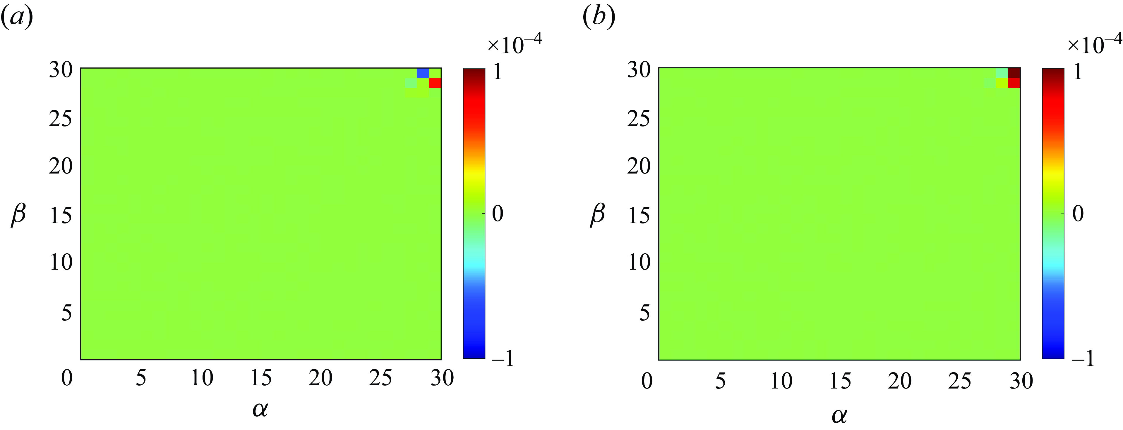
The
 $\widetilde {T}_{(6,\beta )}^{(6,\alpha )}$
across various rings of the sixth shell for
 $N=10$
at
 $t^*=43.1$
is analysed in figure 13(a), while figure 13(b) explores energy transfer from the rings of the fifth shell to those of the sixth shell for
 $N=10$
at
 $t^*=43.1$
. The horizontal axis and vertical axis represent the sector indices of the giver ring
 $\alpha$
and the receiver ring
 $\beta$
, respectively.
Local ring to ring energy transfers (a)
 $\widetilde {T}_{(6,\beta )}^{(6,\alpha )}$
among various rings of the
 $6_{th}$
shell and (b)
 $\widetilde {T}_{(6,\beta )}^{(5,\alpha )}$
from the rings of the
 $5_{th}$
shell to the rings of the
 $6_{th}$
shell for
 $N=10$
at
 $t^*=43.1$
. The horizontal axis and axis vertical represent the sector index of giver ring
 $\alpha$
and receiver ring
 $\beta$
, respectively.

Normalised conical energy flux
 $\Pi (\psi )/max(\Pi (\psi ))$
for different times at
 $N=10$
. The black star makers represent normalised conical energy flux
 $\Pi (\psi )/max(\Pi (\psi ))$
for steady-state forced MHD at
 $N=11$
with the data originating from Reddy et al. (Reference Reddy, Kumar and Verma2014).

Figure 13 clearly reveals that local ring-to-ring energy transfer predominantly occurs near the equatorial region, specifically within the 29th and 30th sectors. This observation aligns well with the Joule cone depicted in figure 6 and the conical energy flux illustrated in figure 14. Furthermore, figure 6(c) elucidates the Joule cone that demarcates the 30th sector as the energy-containing zone and the 29th sector as the Joule dissipation zone. Our analysis primarily focuses on the receiver rings within the 29th and 30th sectors of the sixth shell. For the receiver ring in the 30th sector, figure 13(b) reveals that
 $\widetilde {T}_{(6,30)}^{(5,30)}$
reaches its maximum value, signifying that energy within the energy-containing zone (30th sectors of the sixth shell) is predominantly transported via radial ring energy transfer (defined as energy transfer within the same sector). Conversely, for the receiver ring in the 29th sector of the sixth shell, the values of
 $\widetilde {T}_{(6,29)}^{(5,30)}$
and
 $\widetilde {T}_{(6,29)}^{(6,30)}$
are markedly higher than
 $\widetilde {T}_{(6,29)}^{(5,29)}$
. This indicates that energy within the Joule dissipation zone is primarily sourced through angular ring energy transfer originating from the energy-containing zone (energy transfer across different sectors is referred to as angular ring energy transfer). This finding provides further validation for quasiequilibrium in § 3.4.1, which posits that joule dissipation is predominantly governed by angular energy transfer mechanisms. Notably, this result contrasts sharply with forced MHD turbulence. In forced turbulence, energy in the dissipation zone is chiefly replenished via radial energy transfer, which surpasses angular transfer by an order of magnitude (as elaborated in Reddy et al. (Reference Reddy, Kumar and Verma2014), their figures 6–8). This divergence arises because forced MHD turbulence is characterised by continuous energy injection, whereas decaying turbulence lacks such input. The absence of energy injection in the latter fundamentally alters the nonlinear interactions, resulting in distinct dynamics between these two scenarios.
Figure 14 illustrates the normalised conical energy flux,
 $\Pi (\psi )/\max (\Pi (\psi ))$
, at various time intervals for
 $N=10$
. The black star markers indicate the normalised conical energy flux,
 $\Pi (\psi )/\max (\Pi (\psi ))$
, for steady-state forced MHD at
 $N=11$
, with the data sourced from Reddy et al. (Reference Reddy, Kumar and Verma2014). The conical energy flux exhibits negative values, signifying energy transfer from equatorial modes towards polar modes. Over time, the energy flux near the equator steadily diminishes, eventually approaching zero. This temporal evolution sharply contrasts with the forced MHD scenario, where the energy flux at
 $\theta = \pi /8$
(near the polar region) remains persistently non-zero. This distinction underscores a fundamental difference in the energy transfer dynamics between decaying and forced MHD turbulence.
3.4.3. Bidirectional energy flux
Energy flux (a)
 $\Pi _T(k)$
, (b)
 $\Pi _{T}(k)_{\parallel }$
and
 $\Pi _{T}(k)_{\bot }$
at different times for
 $N=10$
. (c) The ratio between
 $-\Pi _{T}(k)_{\bot ,min}$
and
 $\Pi _{T}(k)_{\parallel ,max}$
versus Joule cone angle
 $cos \theta$
at different times for different
 $N$
. The colour of the scatter points represents different times, and the corresponding relationship can be viewed via the colourbar on the right-hand side. Distribution of
 $x$
-direction velocity within the
 $x{-}z$
plane at
 $N=10$
for (d)
 $t^*=4.65$
, (e)
 $t^*=26.2$
and (f)
 $t^*=71.1$
.

The energy transport in MHD turbulence plays a crucial role for understanding the dynamics of two-dimensional and three-dimensional turbulence. Figure 15 presents the energy flux spectrum across wavenumbers at different times for
 $N = 10$
. The occurrence of both inverse and direct energy transfer during the decay phase is evident, attributed to the coexistence of two-dimensional and three-dimensional turbulent structures, aligning with previous studies (Celani, Musacchio & Vincenzi Reference Celani, Musacchio and Vincenzi2010; Reddy et al. Reference Reddy, Kumar and Verma2014; Baker et al. Reference Baker, Pothérat, Davoust and Debray2018). As depicted in figure 10(d−f), the Lorentz force remains dominant at large scales, indicating that the energy transferred upward is primarily dissipated through Joule dissipation rather than forming large-scale coherent structures (Xia et al. Reference Xia, Byrne, Falkovich and Shats2011).
Additionally, the distribution of
 $\Pi _T(k)_{\bot }$
and
 $\Pi _T(k)_{\parallel }$
across wavenumbers is depicted in figure 15(b). It is evident that
 $\Pi _T(k)_{\bot }$
governs the upward transport of energy, while
 $\Pi _T(k)_{\parallel }$
controls the downward energy transfer, consistent with the findings of Reddy et al. (Reference Reddy, Kumar and Verma2014). Moreover, figure 15(c) shows the relationship between the energy flux ratio
 $|\Pi _T(k)_{\bot ,min}/\Pi _T(k)_{\parallel ,max}|$
and the Joule cone angle
 $\cos \theta$
at different interaction numbers, where the colour of the scatter points represents time. The Joule cone angle characterise the degree of two-dimensionalisation of the flow. It is clear that as time progresses, the Joule cone angle gradually increases (i.e.
 $\cos \theta$
decreases), and the flow tends to become more quasi-two-dimensional (as shown in figure 15
d−f), with the overall three-dimensionality of the flow structure weakening. Simultaneously, as this process advances, the inverse energy flux relative to the direct energy flux gradually increases, i.e. the energy flux ratio gradually rises. It is worth noting that although scatter points do not collapse onto a single line, under the same interaction number, as time decays, the energy flux ratio follows the scaling law
 $|\Pi _T(k)_{\bot ,min}/\Pi _T(k)_{\parallel ,max}|\sim (\cos \theta )^{-2.2}$
.
Thus, the inverse energy cascade is strongly influenced by the degree of two-dimensionality of the flow, with a higher degree of two-dimensionality resulting in a greater proportion of inverse energy transfer. Overall, both turbulence dimensionality and dissipation mechanisms significantly affect the direction of energy transport.
4. Conclusions
The present study investigates the free decay of MHD homogeneous turbulence in a computational box sufficiently large to minimise the effects of periodic boundary conditions. The Joule cone is used to characterise the anisotropy of the turbulence. In all simulations, the Joule cone angle begins its opening at
 $t = \tau (N)$
, demonstrating a scaling law of
 $\cos \theta \sim t^{-1/2}$
, thereby validating Moreau’s theory (Moreau Reference Moreau1990). During the nonlinear stage, small-scale eddies recover to restore three-dimensionality. The state at which the flow ceases to be quasi-two-dimensional and begins to regain isotropy is referred to as the critical state, and it satisfies the condition
 $\gamma (k)=\cos \theta _k T_{\nu }(k)/T_{j}(k)\approx\ {\rm critical\ constant}=0.0062$
. When the flow approaches this critical state, the scale structure shifts from quasi-two-dimensionality to three-dimensionality. Additionally, in the linear stage, the decay law
 $K \sim (t/\tau )^{-1/2}$
is observed to manifest in different zones at different times in Fourier space for the first time. Moreover, it is noteworthy that a decay law of
 $K \sim (t/\tau )^{-3}$
emerges in the nonlinear stage in zones 2 and 3, thus confirming the assumptions proposed by Nihoul (Reference Nihoul1966).
The nonlinear dynamical process in MHD free-decay turbulence has been studied. During the decay, the pressure redistributes energy from velocity components parallel to the magnetic field to those perpendicular, inevitably inducing radial motion in physical space. Furthermore, we find that energy within the energy-containing zone is predominantly transported via radial ring energy transfer. In contrast, energy within the Joule dissipation zone is primarily sourced through angular ring energy transfer, originating from the energy-containing zone. When the interaction number
 $N \gg 1$
, numerical simulations reveal an interval in wavenumber space where the Lorentz force and inertial force are approximately equal, resulting in a
 $k^{-3}$
scaling law in the energy spectrum. This indicates a quasiequilibrium state between angular energy transfer and Joule dissipation in the inertial subrange (Alemany et al. Reference Alemany, Moreau, Sulem and Frisch1979). However, as turbulent energy gradually decays, this quasiequilibrium state is disrupted by viscous effects. And for small scales, the energy spectrum becomes increasingly steeper over time due to the enhanced influence of viscous forces and the gradual reduction of direct energy flux. Furthermore, we observe that the energy spectrum of decaying MHD turbulence also conforms to the exponential spectrum model proposed by Verma & Reddy (Reference Verma and Reddy2015),
 $E(k) \sim \exp (-bk)$
. However, the parameter
 $b$
not only depends on the interaction number
 $N$
but also varies with time. Notably, our simulations observe bidirectional energy transfer, with inverse energy transport largely influenced by the degree of two-dimensionality of the flow, a higher degree of two-dimensionality corresponds to a greater proportion of inverse energy transfer. Under the same interaction number, as time decays, the energy flux ratio follows the scaling law
 $|\Pi _T(k)_{\bot ,min}/\Pi _T(k)_{\parallel ,max}|\sim (\cos \theta )^{-2.2}$
.
Funding
The authors acknowledge the support from CAS under Grants no. YSBR-087, no. XDB0790103.
Declaration of interests
The authors report no conflict of interest.
Appendix A. Validation of dynamic LES for MHD turbulence
Knaepen & Moin (Reference Knaepen and Moin2004) demonstrated that the dynamic LES method is capable of accurately predicting MHD turbulence, as well as its effectiveness in predicting hydrodynamic turbulence. In this appendix, we validate the accuracy of dynamic LES for MHD turbulence using the finite volume method, building upon the framework established in Knaepen & Moin (Reference Knaepen and Moin2004). We also investigate whether dynamic LES can accurately capture the anisotropy of MHD turbulence energy and flux at the poles and equator. The velocity field is initialised in spectral space, and the initial energy spectrum is given as follows:
 \begin{equation} E(k)=C_k \epsilon ^{2/3}k^{-5/3}(\frac {kl}{((kl^{2})+C_l)})^{1/2}\exp(-5.2(k\eta )^4-0.4) .\end{equation}
Here,
 $C_k = 1.5$
,
 $C_L = 6.783$
. All DNS simulations are conducted in a
 $(2\pi )^3$
cyclic box with a resolution of
 $512^3$
, and the viscosity is set to
 $\nu = 0.0003$
. The LES resolution is
 $64^3$
, with the cutoff wavenumber placed in the inertial subrange. Other relevant quantities for the initial field are summarised as follows:
 \begin{align}&\,\,\, Re_L=\frac {u_0L_0}{\nu }=401 , \end{align}
 \begin{align}& Re_{\lambda }=\sqrt {\frac {15}{\epsilon \nu }}u_0^2=81.94 , \end{align}
 \begin{align}&\,\,\, T_{eddy}=\frac {L_0}{u_0}=1.908 . \end{align}
Time history of the resolved kinetic energy density: LES versus filtered DNS. The solid lines represent the predictions of the DSM, and the stars represent the filtered kinetic energy density obtained by truncating the DNS fields to a
 $64^3$
resolution.

Here,
 $u_0$
,
 $L_0$
and
 $\epsilon _0$
represent the initial field’s velocity fluctuations, integral scale and viscous dissipation, respectively. For the LES cases, the initial field is obtained by filtering the DNS results. We have set up four cases in total, which include two DNS cases (with
 $N=0$
and
 $N=10$
) and two LES cases (similarly with
 $N=0$
and
 $N=10$
).
Three-dimensional kinetic energy spectra for the case
 $N=0$
at different times. The solid line represents DSM and the dashed line represents filtered DNS. The specific times at which the spectra are calculated are indicated in the plots.

Three-dimensional kinetic energy spectra for the case
 $N=10$
at different times. The solid line represents DSM and the dashed line represents filtered DNS. The specific times at which the spectra are calculated are indicated in the plots.

The spectrum of
 $E(\psi )$
for the case
 $N=10$
at different times (a)
 $N=0$
and (b)
 $N=10$
. The solid line represents DSM and the dashed line represents filtered DNS. The specific times at which the spectra are calculated are indicated in the plots.

Here
 $\Pi _{\theta }$
for the case
 $N=10$
at different times. The solid line represents DSM and the dashed line represents filtered DNS. The specific times at which the spectra are calculated are indicated in the plots.

Figure 16 shows the time evolution of the resolved kinetic energy predicted by the DSM, compared with the filtered DNS results. The
 $N=0$
case serves as a benchmark, confirming that for non-conductive flows, our LES code behaves as expected. For
 $N=10$
, the DSM model performs exceptionally well. Figures 17 and 18 present the kinetic energy spectra for both
 $N=0$
and
 $N=10$
cases at various time steps, demonstrating excellent agreement between the LES with dynamic procedure and DNS results.
To further assess whether dynamic LES captures the MHD turbulence anisotropy, figures 19 and 20 show the spectra of
 $E(\psi )$
and
 $\Pi (\psi )$
for the
 $N=10$
case at different times. Here,
 $E(\psi _0) = \sum _{\psi = \psi _0} E(k,\phi ,\psi )$
, where
 $(k, \phi , \psi )$
are spherical coordinates in Fourier space. The results show that the LES predictions align closely with the filtered DNS, confirming that dynamic LES can accurately predict MHD turbulence, including the pole–equator anisotropy of energy.