1 Introduction
Whilst the study of steady axisymmetric shock wave phenomena is the most dated in the field, research has focused on the effects of conical geometry. The shock wave structures, formed in planar symmetry and straight wedge interactions, have been extensively covered in works such as those by Ben-Dor (Reference Ben-Dor2008). The phenomena involved in steady axisymmetric shock structures have not been explored and detailed to such an extent. Early work was completed by Ferri & Nucci (Reference Ferri and Nucci1951) with the application to supersonic inlets, which has remained the practical focus of internal supersonic axisymmetric flow fields to date. Before the advent of efficient computing, numerical solutions were proposed to axisymmetric and internal conical flow fields using techniques such as the method of characteristics as proposed by Mölder (Reference Mölder1967). Numerical studies, undertaken by Timofeev et al. (Reference Timofeev, Mölder, Voinovich, Takayama, Hosseini, Takayama and Lu2001), later showed how in an axisymmetric case the only reflection type that is possible is that of a Mach reflection. This was due to the fact that the incident shock wave steepens towards the triple point, exceeding the Von Neumann angle. Recent work by Gounko (Reference Gounko2017) has focused on the positioning of the Mach disk in supersonic and axisymmetric flow fields, exploring the influence of longitudinal or transverse curvature due to the axisymmetric nature of the Mach reflection.
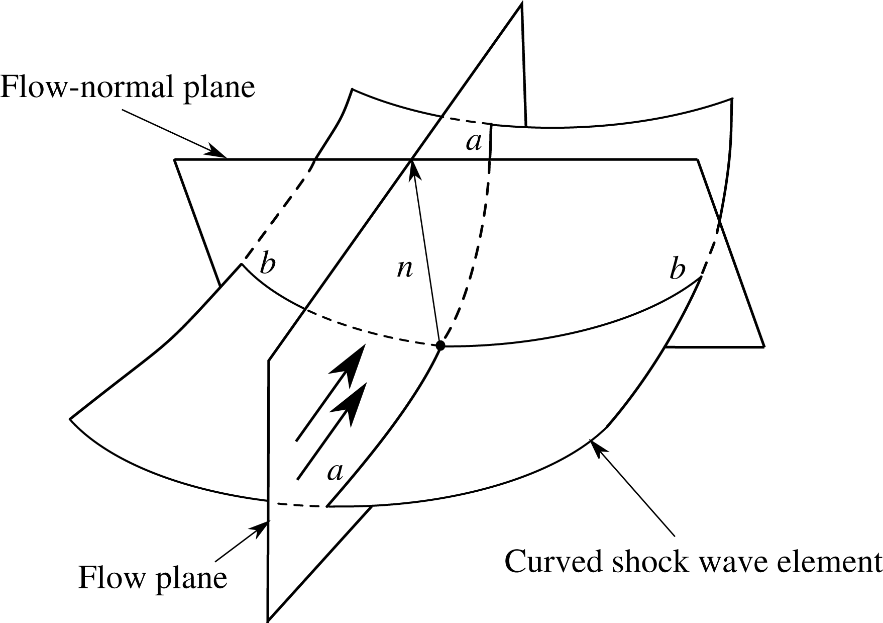
Most research involving supersonic axisymmetric internal flow fields, however, has involved internal surfaces which are only conical in nature. Very little published data has been presented concerning supersonic flow fields originating from concavely curved internal surfaces. Unlike the case of axisymmetric conical internal surface flows, which are only deflected towards the axis of symmetry, supersonic flows deflected by axisymmetric concave internal surfaces are curved by two sources. The first source being the axisymmetry of the deflection, like the conical case, and the second source being the internal surface curvature, which compressively turns the flow inwards. In figure 1, for a steady supersonic flow entering a stationary shock element, the shock traces in the flow and flow-normal directions are defined as
 $a{-}a$
and
 $b{-}b$
respectively. The flow plane curvature is the geometric curvature of the curved shock wave, dependent on the function that describes the shock trace
 $a{-}a$
. The transverse curvature or flow-normal plane curvature is equivalent to
 $-\cos \unicode[STIX]{x1D703}/y$
, where
 $\unicode[STIX]{x1D703}$
denotes the shock angle and
 $y$
denotes the perpendicular distance from the axis of symmetry to the point of interest (Mölder Reference Mölder2016). If the compressive waves that change the shock wave shape are no longer being influenced by flow plane deflections, such as internal surface curvature, then the only mechanism by which the shock waves curve would be via the presence of an expansion fan or transverse curvature.
The work contained herein examined the effect of varying the internal surface’s radius of curvature and leading-edge angle of axisymmetric ring wedges. This has a resulting influence on the shock wave structures and flow fields. To the writers’ knowledge no data has been published to date concerning these interactions.
Curved shock wave element adapted from Mölder (Reference Mölder2016).

2 Experimental set-up
2.1 Supersonic wind tunnel facility
The blowdown supersonic wind tunnel facility at the University of the Witwatersrand, Johannesburg, allowed for the completion of the experimental work. Experimental tests were completed between Mach numbers of 2.8 and 3.6 in a test section whose cross-sectional dimensions measure 101.6 mm
 $\times$
101.6 mm. U-configuration shadowgraph and schlieren flow visualisation was used to capture features in the flow field and provide qualitative flow data, using a eight-megapixel Canon EOS 350D camera and a Xenon flash lamp with a
 $1.5~\unicode[STIX]{x03BC}\text{s}$
exposure time.
2.2 Experimental ring wedge models
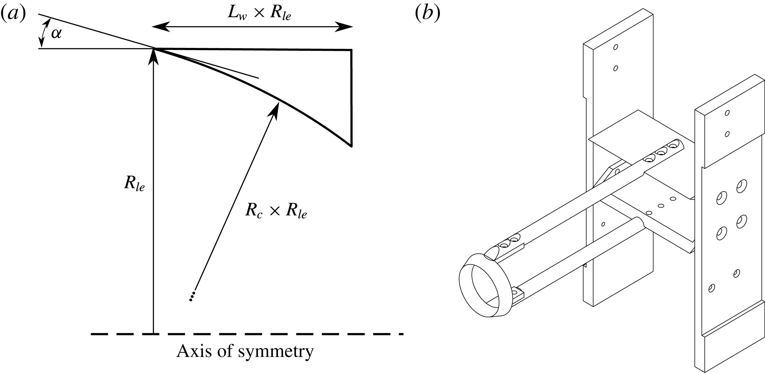
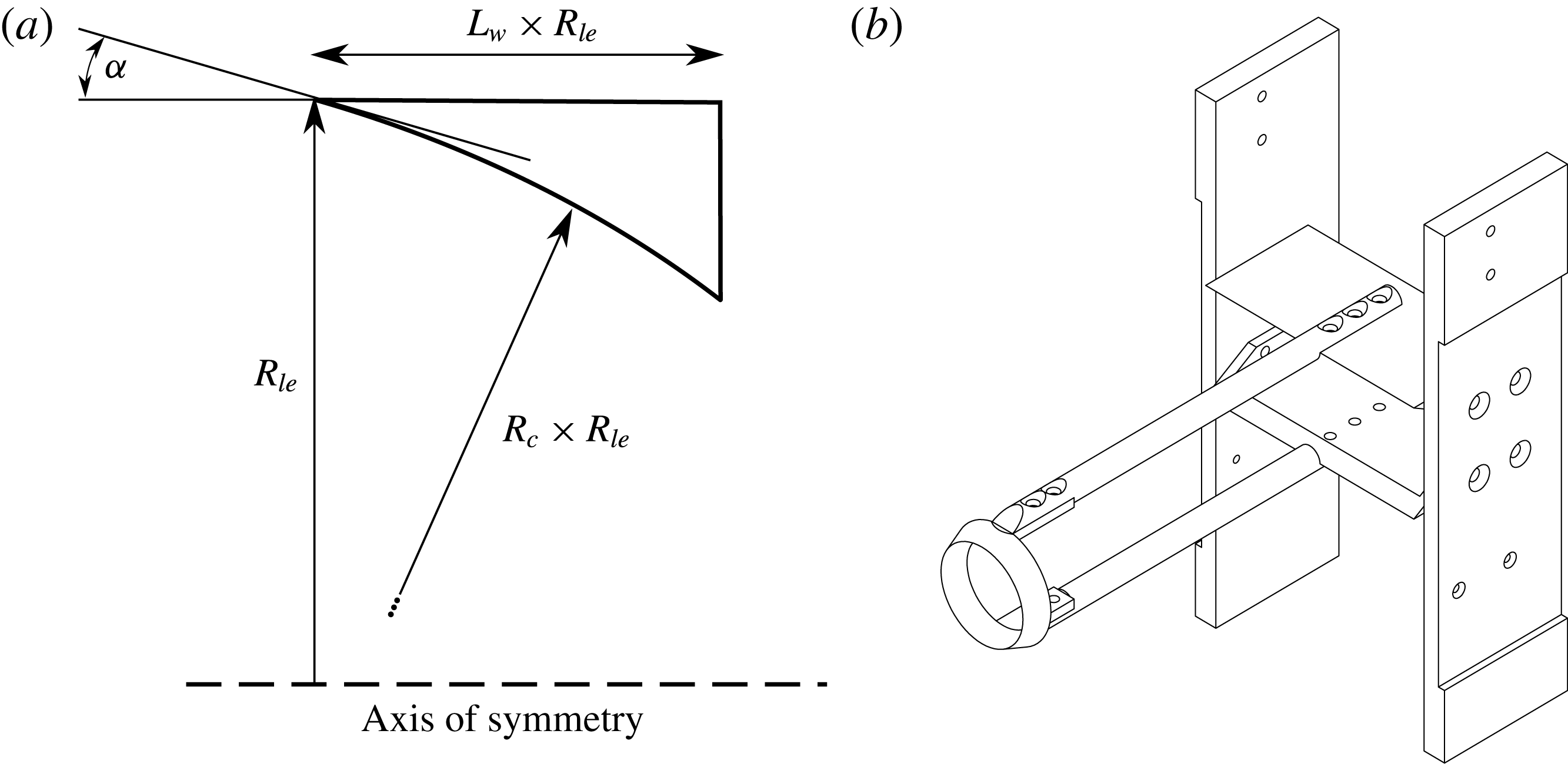
Ring wedge models were manufactured for the purposes of experimental testing. Referring to figure 2(a), all the dimensions of the ring wedge are normalised with respect to the leading-edge radius,
 $R_{le}$
, and where
 $R_{c}$
denotes the normalised internal radius of curvature,
 $L_{w}$
the normalised ring wedge length and
 $\unicode[STIX]{x1D6FC}$
the leading-edge angle. The leading-edge radius was set to
 $R_{le}=20~\text{mm}$
and the wedge length to 10 mm (therefore,
 $L_{w}=10/R_{le}=0.5$
) after initial parameter studies were undertaken due to spatial constraints that caused wind tunnel choking. Experimental parameters were varied for radius normalised internal radii of curvature of
 $R_{c}=\{1,1.5,2\}$
and leading-edge angles of
 $\unicode[STIX]{x1D6FC}=\{0^{\circ },4^{\circ },8^{\circ }\}$
.
A new model support and experimental models were designed in order to carry out the experimental component of the research as seen in figure 2(b). This provided a rigid support for the ring wedge while keeping the flow field unobscured so that the shock structure and features behind the ring wedge could be seen. Issues were encountered during experimental testing due to the formation of a separated flow region during wind tunnel start up. This caused an unstable oblique shock to travel downstream and detach shock structures for cases where the axisymmetric flow contraction was high. This resulted in a bow shock remaining on the model where an attached shock numerically existed. These cases are not considered – only those where stable flow is present have been presented.
Experimental schematics. (a) Ring wedge parameters; (b) test model assembly.
3 Numerical set-up
Due to the physical axisymmetric geometry of the ring wedge model it is not possible to visualise what is occurring within it. Only the flow field behind the ring wedge can be seen as the internal flow field is hidden from view. The usage of numerical methods can lead one to analyse the shock structure and flow properties as a direct result of the internal surface curvature.
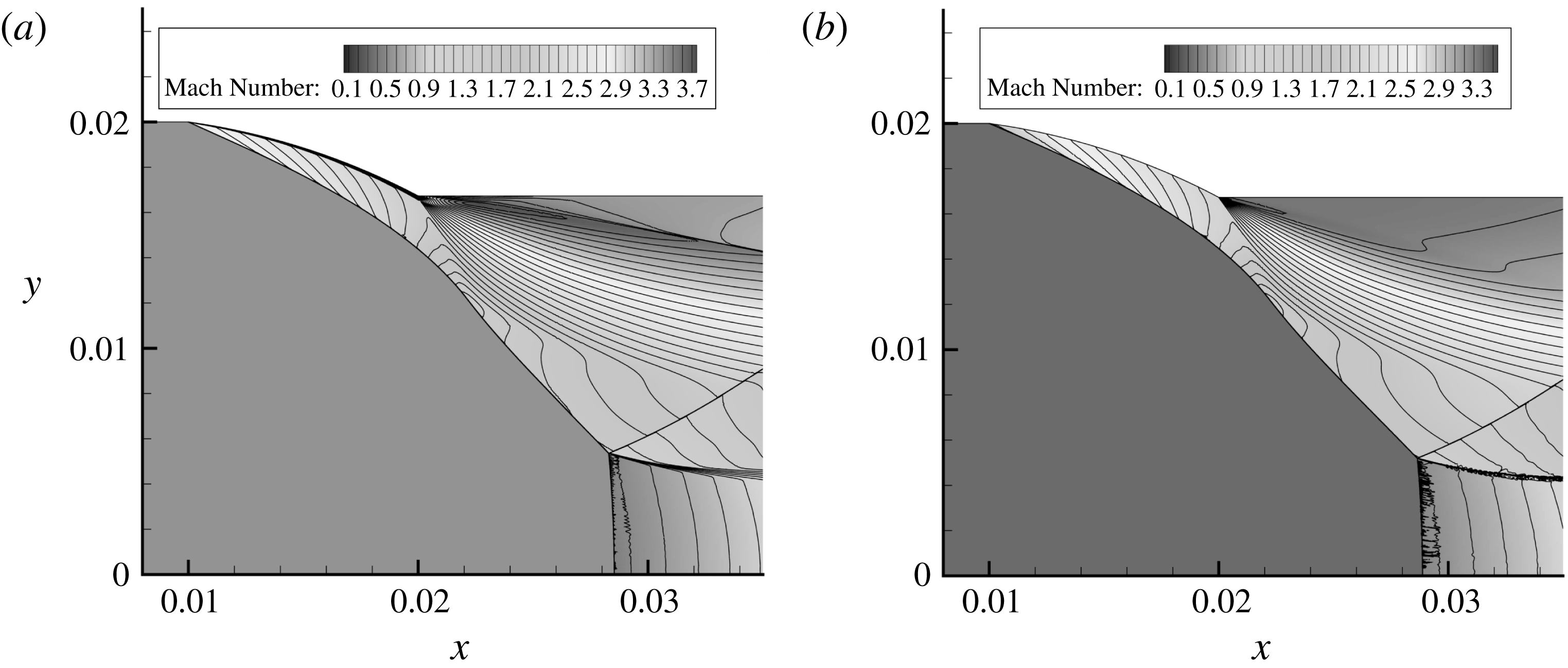
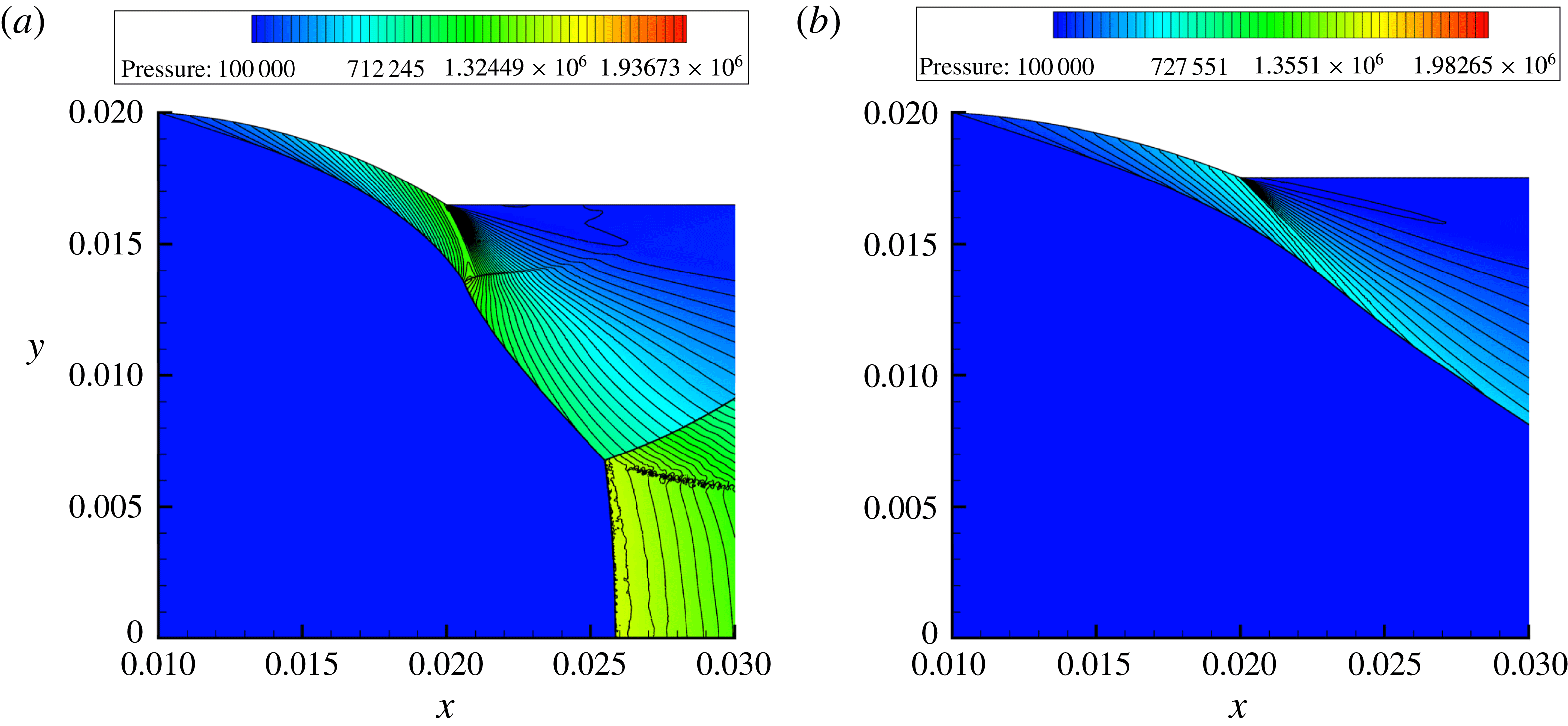
Euler equation formulations in ANSYS Fluent 15.0 were used to obtain CFD simulation results as the effects of viscosity and the presence of a supersonic boundary layer were deemed negligible. This is shown using figure 3, where a viscous and an Euler formulation are compared. The viscous equation formulation employed the
 $\unicode[STIX]{x1D705}{-}\unicode[STIX]{x1D714}$
SST turbulence scheme in order to provide results in comparison to the same ring wedge model under Euler conditions. The overall flow field remained relatively unchanged except for a 0.36 mm shift in the shock structure positioning. This shift does not change the influence of the internal surface curvature or the leading-edge angles. Since the study is limited to one of a qualitative nature, the same flow altering effects are seen in either case. The shock structure shift caused by the effects of viscosity and boundary layer presence was determined to be of little importance in the context of the current study.
Two-dimensional axisymmetric computational domains were created for each ring wedge in question and were simulated for each experimental parameter set. The computational domain was discretised using the standard CFD meshing algorithms built into ANSYS 15.0, with uniform quadrilateral cell sizing of 0.1 mm being applied to the domain. Wall boundaries were applied to the internal surface of the ring wedges models while non-reflective pressure far-field boundary conditions where applied to all other non-axis boundaries. This was done in order to stop the formation of unwanted additional internal boundary shock reflections emanating from the resulting shock structure, thereby mimicking the experimental conditions. Dynamic adaptive meshing techniques were employed to locate and refine the shock structures, using refinement levels and thresholds, which were found to produce sufficiently resolved flow features to a final cell size of
 $1.5625~\unicode[STIX]{x03BC}\text{m}$
. All numerical solutions that are presented underwent grid sensitivity studies for mesh grid independence and were continued until their iterative convergence. The simulation results were then post-processed using Tecplot 360 EX 2014 Release 1.
 $R_{c}=1.5$
,
 $\unicode[STIX]{x1D6FC}=8^{\circ }$
,
 $L_{w}=0.5$
model at Mach 3.4. (a) Viscous equation formulation using the
 $\unicode[STIX]{x1D705}{-}\unicode[STIX]{x1D714}$
SST turbulence scheme. (b) Euler equation formulation.
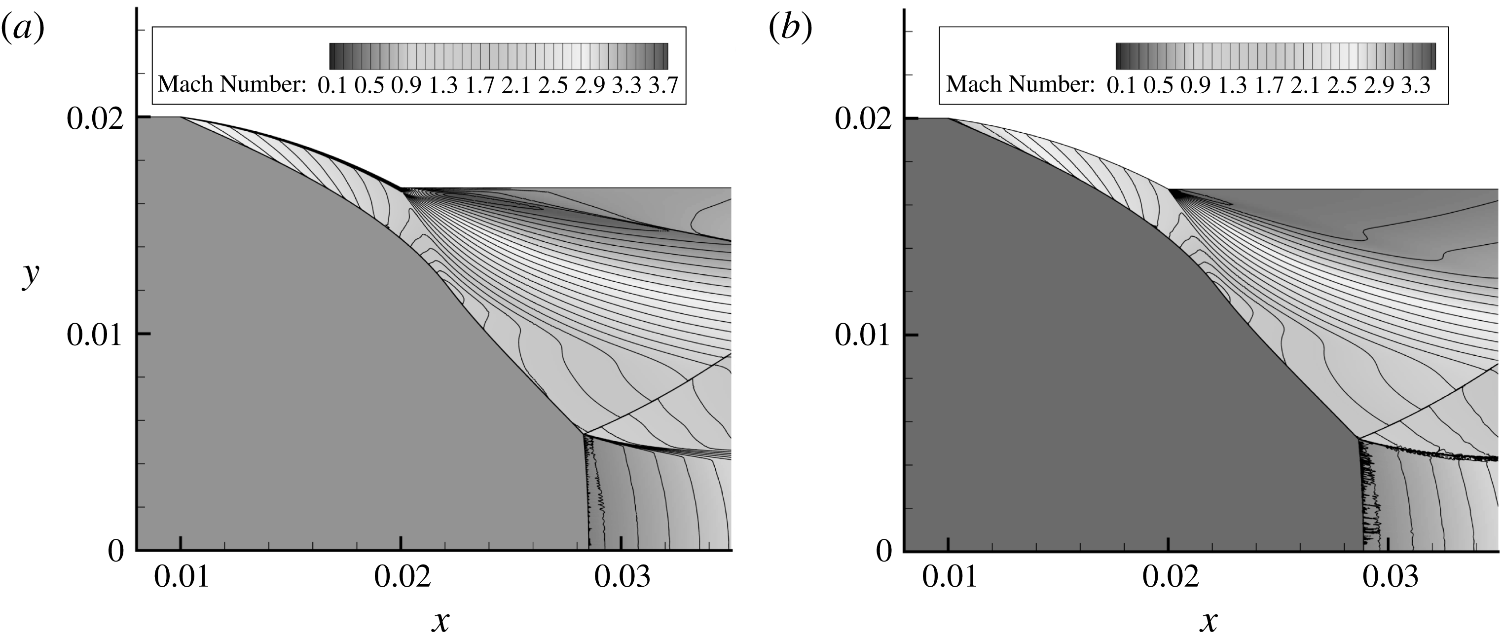
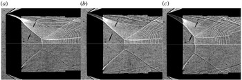
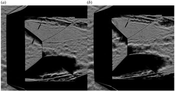
Figure 4 displays comparative experimental shadowgraph results overlaid with their corresponding numerical CFD results. The experimental and numerical results were found to be in excellent agreement with one another. The differences that are more apparent are in the region of the reflected shock wave that originates from the Mach reflection triple point. As the reflected shock stretches from the triple point it is altered by the trailing-edge expansion wave fan and shock wave interactions emanating from the test rig. Said flow features divert and curve the reflected shock wave very slightly. Since the image plane is in the same plane as the ring wedge model rod supports, their flow interactions and subsequent effects on the reflected shock wave are captured.
Experimental with overlaid CFD results. (a)
 $R_{c}=1,\unicode[STIX]{x1D6FC}=0^{\circ },L_{w}=0.5$
model at Mach 3.6; (b)
 $R_{c}=1.5,\unicode[STIX]{x1D6FC}=4^{\circ },L_{w}=0.5$
model at Mach 3.2; (c)
 $R_{c}=2,\unicode[STIX]{x1D6FC}=8^{\circ },L_{w}=0.5$
model at Mach 2.8.

4 Results and discussion
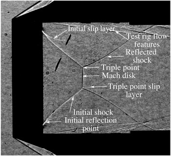
Figure 5 contains the naming convention used and assigned to certain flow features mentioned throughout § 4.
General flow feature naming convention.

4.1 Effect of varying internal surface curvature
4.1.1 Leading-edge angle
 $\unicode[STIX]{x1D6FC}=0^{\circ }$

When
 $\unicode[STIX]{x1D6FC}=0^{\circ }$
the flow field and shock waves that form are controlled purely by the internal surface curvature. A shock wave does not start from the leading edge but is replaced by an isentropic compression which coalesces into a shock wave downstream. The compression waves from the internal surface fan inwards and cause the shock wave to curve as they each interact with the shock structure. The angle of these compression waves is determined by the flow speed and deflection caused by the internal surface. Since an axis of symmetry is involved, the flow plane is rotated around said axis and is additionally curved due to this rotated dimensionality. This causes the compression waves, which emanate from the wall, to be curved so their influence cannot be predicted easily using analytical methods.
Considering the change in internal surface curvature, as
 $R_{c}$
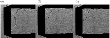
increases the internal surface curvature decreases since the radius of curvature increases. This affects how the shock wave in the internal flow field of the ring wedge models form as the compression waves that control their shape are driven by the surface curvature of the wall. Figure 6(a–c) displays the shadowgraphs of the
 $R_{c}=1,R_{c}=1.5$
, and
 $R_{c}=2$
models, respectively, where
 $\unicode[STIX]{x1D6FC}=0^{\circ }$
at Mach 3.0.
Experimental shadowgraph results. (a)
 $R_{c}=1,\unicode[STIX]{x1D6FC}=0^{\circ }$
model at Mach 3.0; (b)
 $R_{c}=1.5,\unicode[STIX]{x1D6FC}=0^{\circ }$
model at Mach 3.0; (c)
 $R_{c}=2,\unicode[STIX]{x1D6FC}=0^{\circ }$
model at Mach 3.0.

Many differences are apparent between the different surface curvature cases. Firstly, examining the existence of an initial slip layer forming on the initial shock just downstream from the back of the model, it can be seen that it is stronger in the
 $R_{c}=1$
case. Increasing
 $R_{c}$
to 1.5, the visibility of the initial slip layer is low, however, it can still be seen very faintly with magnification into the image. Finally at
 $R_{c}=2$
the slip layer is not visible. The visibility and strength of the initial slip layer is governed by the ratio of flow velocities across it. The higher the value of
 $R_{c}$
the more the shock wave and flow field is curved. This causes the post-shock flow speed to decrease further than it would at higher
 $R_{c}$
values. The stronger the influence of the curvature and the trailing-edge expansion fan, the greater the velocity ratio across the slip layer, the more pronounced it is.
The additional flow features in figure 6(a), at the top and bottom of the model, out of the reflection zone, are formed by the test rig. These test rig flow features are created due to wake forming behind the test rig and interacting with the connecting mounts. The expansion fan, which is reflected in onto itself by the arms that extend out the trailing-edge surface, which connect to the rod supports, now becomes compressive in nature and forms additional test rig flow features. Said features cannot influence the flow of interest.
Returning to the comparison between the different curvatures involved, the differences in location on the Mach disk are as a result of the angle of the initial shock pointing downstream. The flow leaving the ring model is deflected through a greater angle as
 $R_{c}$
decreases. Therefore, the incident shock of the Mach reflection is steeper. This will then affect the progression of the Mach disk further downstream. The change in
 $R_{c}$
will additionally change the size of the angle through which the flow must adjust via the expansion fan. The smaller the value of
 $R_{c}$
, the larger the internal surface curvature. This means the angle between the tangent of the internal surface and wake of the trailing edge is larger as the tangent becomes steeper with decrease in
 $R_{c}$
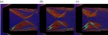
. This increase in angle through which the flow expands via the expansion fan will correlate to a larger pressure ratio across the expansion fan, increasing its strength and influence. The difference in the expansion wave fan strength for
 $\unicode[STIX]{x1D6FC}=0^{\circ }$
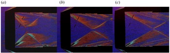
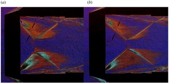
models at Mach 3.4 can be seen in figure 7(a–c) using colour mask schlieren techniques. The expansion fan is clearer on the bottom trailing edge.
Colour mask schlieren results. (a)
 $R_{c}=1,\unicode[STIX]{x1D6FC}=0^{\circ }$
model at Mach 3.4; (b)
 $R_{c}=1.5,\unicode[STIX]{x1D6FC}=0^{\circ }$
model at Mach 3.4; (c)
 $R_{c}=2,\unicode[STIX]{x1D6FC}=0^{\circ }$
model at Mach 3.4.

In figure 7(a),
 $R_{c}$
is at the minimum value of 1; therefore, the internal surface has more curvature. This would mean that the flow has to pass around the largest angle of the three cases at the trailing edge, resulting in the strongest expansion fan. The angle being measured from the first expansive Mach line to the influence of the wake’s orientation which is governed by the base pressure. The pressure ratio for the
 $R_{c}=1$
case would be the largest as the pressure before the corner is at a maximum due to the increased surface curvature, increasing the compression. This is confirmed by examining the relative size of the expansion fans and density gradients displayed in figure 7(a–c). The larger the value of
 $R_{c}$
, the weaker the expansion, and therefore a smaller-sized affected region is seen in the density gradients. Since the internal surface curvature directly controls the deflection, it governs what speed the flow exits the ring wedge. This then controls the angle of the first expansive Mach line, which makes up part of the expansion fan, and controls what direction it originally starts at. The slower the flow, the steeper the angle, causing the expansion fan to interact with the initial shock sooner. Additional convexity is then introduced into the initial shock wave, curving it, and therefore inhibiting its ability to propagate further downstream.
The comparative density gradients behind the initial shocks in each
 $R_{c}$
case can be visualised by the amount a region deviates from the purple background into the orange and red bands of the horizontal lattice mask used in the colour mask schlieren set-up. The lack of symmetry between the orange and red regions is due to a slight vertical offset of the colour mask favouring the red band. The relative strength between the initial shock waves can be seen by the size of the red and orange regions behind the initial shock wave. This dictates how much light it refracted by the changes in air density, causing it to pass through the different colour bands. For the
 $R_{c}=1$
case one would expect the shock wave leaving the internal ring wedge section to be steeper due to the increased flow deflection it experiences in comparison to the
 $R_{c}=1.5$
and
 $R_{c}=2$
cases. Its strength would then be comparatively higher, which can be seen as the flow field behind the initial shock in figure 7(a) is filled by more red and orange colour regions relative to figure 7(b,c).
With the change in
 $R_{c}$
affecting the orientation of the expansion fan, the effect of transverse curvature may be impacted. Transverse curvature is brought about by wall convergence. Flow plane or longitudinal curvature is brought about by wall turning. Both, when being towards the axis of symmetry, will cause flow area reduction and supersonic flow compression. In the
 $R_{c}=1$
case the expansion fan causes the initial shock to become convex, as evident in figure 7(a). This convexity bends the shock away from the axis of symmetry, thereby counteracting the effects of transverse curvature which rely on proximity to said central axis as well as the shock angle. The further downstream the reflection moves, the more apparent the effect of transverse curvature. With distance from the trailing edge the influence of the expansion fan is weakened and so it loses its ability to combat and oppose the onset of concavity in the shock wave due to transverse curvature. Its effects then become more pronounced.
Mach number does not have as great an impact on the formation of the shock wave structures in comparison to varying the internal surface curvature. Since the internal surface remains constant for each ring wedge, by increasing Mach number all that is achieved is the variation of the angles of the compression waves that curve the shock wave. The higher the Mach number, the more swept back they are. This causes the shock to curve to a greater extent further downstream, creating a more gentle angled initial shock wave, sending the Mach reflection to a more downstream position.
4.1.2 Leading-edge angle
$\unicode[STIX]{x1D6FC}=4^{\circ }$

With the value of the leading-edge angle,
 $\unicode[STIX]{x1D6FC}$
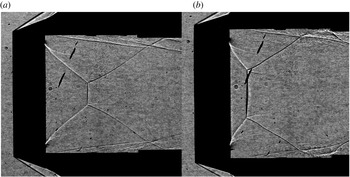
, being increased to a non-zero value, an initial deflection exists at the leading edge. An attached shock now extends from the leading edge which will be curved by the wall-emanating compression waves. Examining the initial reflection slip layer that was previously mentioned, figure 8(a,b) displays shadowgraphs for the
 $R_{c}=1$
and
 $R_{c}=1.5$
,
 $\unicode[STIX]{x1D6FC}=4^{\circ }$
models, respectively, at Mach 3.6.
Experimental shadowgraph results. (a)
 $R_{c}=1,\unicode[STIX]{x1D6FC}=4^{\circ }$
model at Mach 3.6; (b)
 $R_{c}=1.5,\unicode[STIX]{x1D6FC}=4^{\circ }$
model at Mach 3.6.

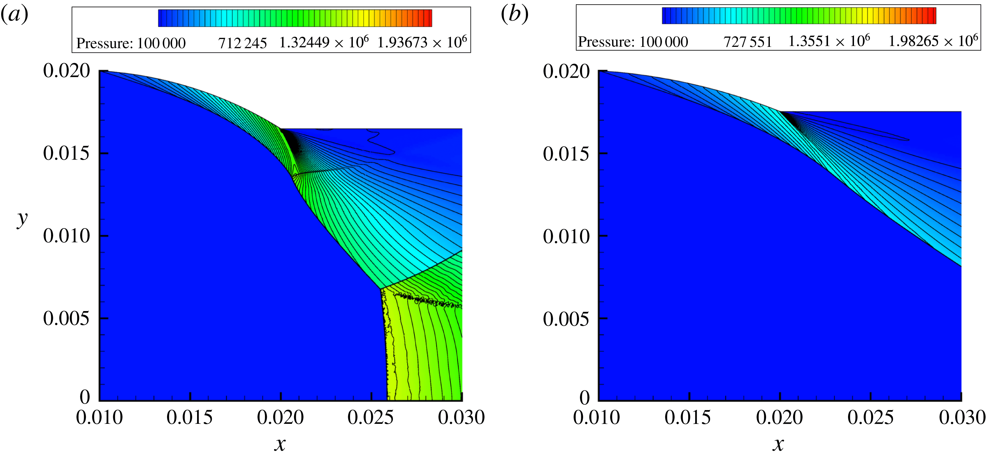
Numerical pressure contour results. (a)
 $R_{c}=1,\unicode[STIX]{x1D6FC}=4^{\circ }$
model at Mach 3.6; (b)
 $R_{c}=1.5,\unicode[STIX]{x1D6FC}=4^{\circ }$
model at Mach 3.6.
For the
 $R_{c}=1$
model in figure 8(a) the initial slip layer is still very pronounced, whereas in figure 8(b) it is barely visible for the
 $R_{c}=1.5$
case. Their presence must therefore be a function of
 $R_{c}$
, as previously suggested. Since the initial slip layer is present in a case where
 $\unicode[STIX]{x1D6FC}=4^{\circ }$
it is not a product of the isentropic compression to shock wave transformation of the
 $\unicode[STIX]{x1D6FC}=0^{\circ }$
case either. Its formation must then be linked to the way the flow is deflected in each
 $R_{c}$
separate case. A shock wave reflection exists to realign supersonic flow; therefore, the excess deflection, caused by lower values of
 $R_{c}$
increasing the internal surface curvature, causes the flow to want to turn in onto itself. This then must be corrected so a reflection forms. This can be confirmed by examining the shapes of the compression waves emanating from the wall.
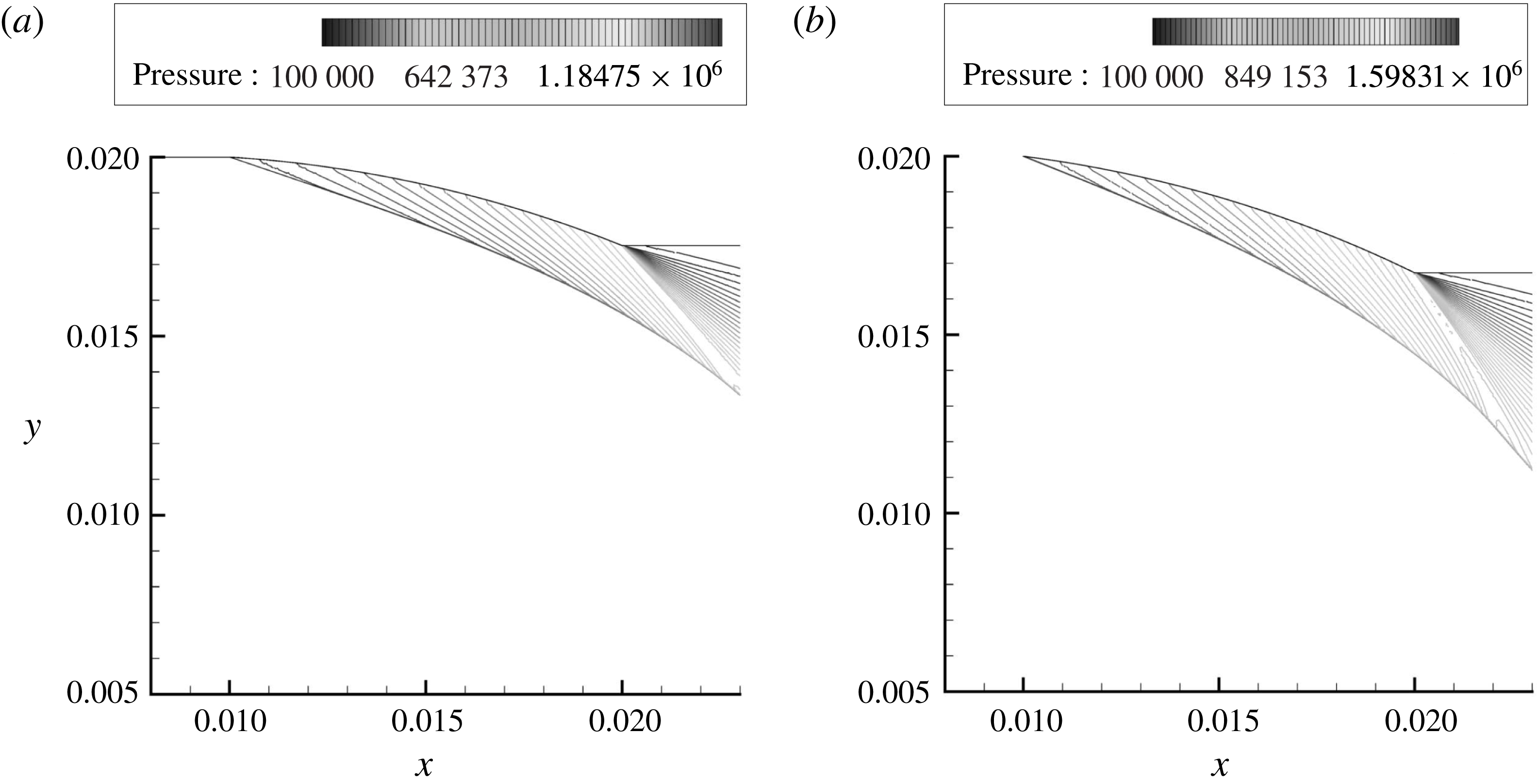
The pressure contours for the
 $R_{c}=1$
and
 $R_{c}=1.5$
,
 $\unicode[STIX]{x1D6FC}=4^{\circ }$
models at Mach 3.6 are displayed in figure 9. These two cases match figure 8(a,b), where the initial slip layer is present for the
 $R_{c}=1$
model, meaning a very weak shock must exist. A slip layer itself is isobaric so no pressure difference exists across its boundary, hence they are not visible in figure 9. The only reason a slip-layer-like feature exists in figure 9(a) at the Mach reflection triple point is due to numerical instabilities that arise from a Kelvin–Helmholtz instability forming and being over-refined by sensitive mesh adaptation criteria. The location of the slip layer is given by the placement of a weak initial reflected shock in figure 9(a). The compression waves which are represented by the pressure contours show how they shape and turn a curved shock wave with progression along the internal curved surface. These compression waves are dependent on the incremental change in flow deflection along the internal wall surface. Therefore, since the internal surface is curved and not stepped, there exists an infinite number of compression waves as there does an infinite number of increments into which the deflection along a curved wall can be broken into. The closer one moves down the initial shock towards the first reflection point, the compression waves can be seen to change direction and curve upstream slightly. This occurs directly before the initial reflection point as the compression waves turn from pointing downstream and begin to bend upstream, meaning the flow is beginning to turn in on itself. Therefore, the large flow deflection and curvature imposed by the
 $R_{c}=1$
internal surface, coupled with transverse curvature, is causing the compression waves to bend in on themselves and form a weak reflection and the initial slip layer. In comparison, the compression waves of figure 9(b) only extend downstream. They do not bend inwards onto themselves, causing no reflection to form as the imposed curvature is not high enough. This explains the absence of the initial slip layer and weak initial reflected shock given the Mach number of the post-curved shock flow.
4.1.3 Leading-edge angle
$\unicode[STIX]{x1D6FC}=8^{\circ }$

With
 $\unicode[STIX]{x1D6FC}$
at its maximum value of
 $8^{\circ }$
the leading-edge shock is now at its steepest. Due to the increased exit area contraction in the
 $R_{c}=1,\unicode[STIX]{x1D6FC}=8^{\circ }$
model, it was not possible to experientially or numerically test it given the current study’s Mach number range. Issues outlined in § 2 hindered the experimental gathering of results below Mach 3.4 for the
 $R_{c}=1.5,\unicode[STIX]{x1D6FC}=8^{\circ }$
model. Figure 10(a,b) displays colour mask schlieren results for the
 $R_{c}=1.5$
and
 $R_{c}=2,\unicode[STIX]{x1D6FC}=8^{\circ }$
models, respectively, at Mach 3.4.
Colour mask schlieren results. (a)
 $R_{c}=1.5,\unicode[STIX]{x1D6FC}=8^{\circ }$
model at Mach 3.4; (b)
 $R_{c}=2,\unicode[STIX]{x1D6FC}=8^{\circ }$
model at Mach 3.4.

With the
 $R_{c}=1.5$
case imposing a larger curvature on the curved shock wave than that of the
 $R_{c}=2$
case, the angle of the initial shock wave is steepened. The same curvature-induced expansion wave strength mechanics that were previously mentioned can be seen to apply in figure 10(a,b). In figure 10(a), where
 $R_{c}=1.5$
, the flow leaving the internal surface passes with a greater angle around the trailing edge so the pressure ratio and strength of the expansion fan is greater in comparison to figure 10(b) where
 $R_{c}=2$
. Due to the additional convexity imposed on the initial shock it becomes more axially symmetrically curved. That is why the pre-initial shock density gradients in figure 10(a) seem larger in size as opposed to those in figure 10(b).
The influence of the size of the Mach disk on the density gradients can be seen in figure 10(a,b). For the
 $R_{c}=1.5$
case the Mach disk is larger as a result of the steepened initial shock and more upstream positioning. The different density gradients regions behind the Mach disk are larger in figure 10(a) than in figure 10(b), and so the strength must differ between the two cases. The larger the Mach disk, the greater the tendency for it to curve, therefore creating larger density gradients within the triple-point slip-layer-bounded streamtube behind it. Although the curvature is very slight and not easily discernible, small differences in curvature can result in larger density gradients. This is due to the nature of a Mach disk being a very strong normal shock wave as the shock angle approaches
 $90^{\circ }$
at the axis of symmetry.
4.2 Effect of leading-edge angle
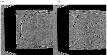
Figure 11(a,b) contains the shadowgraph results for the
 $\unicode[STIX]{x1D6FC}=0^{\circ }$
,
 $\unicode[STIX]{x1D6FC}=4^{\circ }~R_{c}=1$
models, respectively at Mach 3.6. The curvature of the Mach disk can now be seen prominently in figure 11(b) due to its size and thickness. A double image of the Mach disk seems to have formed, but this occurs due to its curved axial symmetry and the shadowgraph technique picking up both the downstream curved shock surface and the upstream frontal surface of the Mach disk. In figure 11(a) the initial shock is not as steep, as the leading edge is tangent to the flow and the internal surface curvature does not curve the shock to as great an extent. This means the Mach reflection forms further downstream and is smaller in size. The curvature of the Mach disk in figure 11(a) is therefore more difficult to visualise in comparison to figure 11(b).
Experimental shadowgraph results. (a)
 $R_{c}=1,\unicode[STIX]{x1D6FC}=0^{\circ }$
model at Mach 3.6; (b)
 $R_{c}=1,\unicode[STIX]{x1D6FC}=4^{\circ }$
model at Mach 3.6.

Since the advent of an increase in
 $\unicode[STIX]{x1D6FC}$
to a non-zero value causes the attached shock to form, the flow bounding the internal surface is slower in velocity than that of an isentropic compression. Therefore, the flow that enters and leaves the initial reflection is at a lower velocity compared to the case where an isentropic compression initially exists and then coalesces into a shock wave. The velocity ratio across the slip layer would then be larger and the appearance of the slip layer would be more prominent and longer. This can be seen when comparing figures 11(a) and 11(b). Firstly, the initial reflection slip layers in figure 11(a) are slightly longer than those in figure 11(b), where
 $\unicode[STIX]{x1D6FC}=4^{\circ }$
. Secondly, the initial slip layer near the lower trailing edge seems to be more prominent in figure 11(a) than in 11(b). This difference in strength causes the slip layer to appear as more prominent and longer. It does not dissipate as soon in the shadowgraph images where
 $\unicode[STIX]{x1D6FC}=0^{\circ }$
, and its discontinuity effects are still captured.
With the full array of experimental and numerical results available with varying
 $\unicode[STIX]{x1D6FC}$
values at
 $R_{c}=1.5$
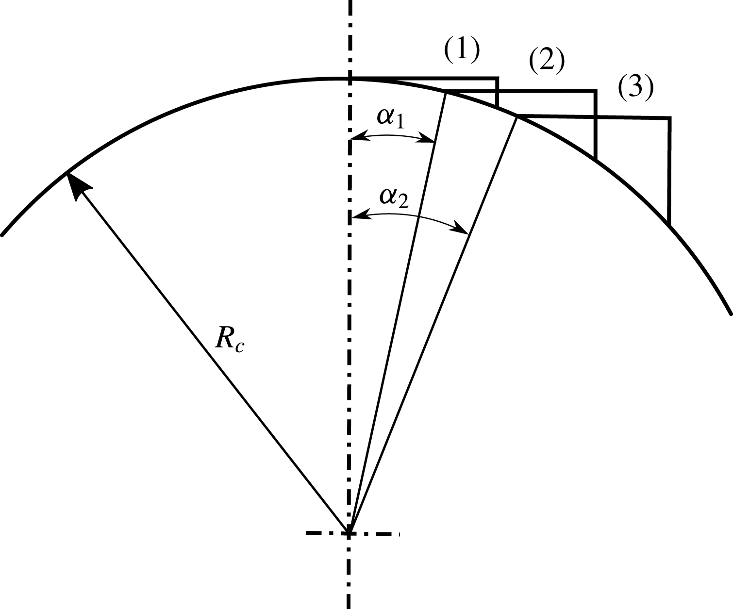
, its overall influence can be more clearly observed. Figure 12 displays the progression of an internally curved wedge along a constant radius arc. When the wedge’s leading edge is tangent to the flow, in the case of
 $\unicode[STIX]{x1D6FC}=0^{\circ }$
, it sits at the top of the arc. As
 $\unicode[STIX]{x1D6FC}$
increases to some non-zero value,
 $\unicode[STIX]{x1D6FC}_{1}$
, the location of the wedge moves along the arc from (1) to (2). Finally, when
 $\unicode[STIX]{x1D6FC}_{2}$
is greater than
 $\unicode[STIX]{x1D6FC}_{1}$
, the wedge is moved to location (3) further along the constant radius arc. During this progression the angle between the tangents to the internal curved surface at the leading and trailing edge remain constant as the wedge moves from (1) to (2) and eventually to (3). The net flow deflection along the internal surface then remains constant as
 $\unicode[STIX]{x1D6FC}$
increases due to the constant radius along the arc. The compression waves that curved the shock wave therefore have to deflect the flow through the same net deflection in each case.
Progression of an internally curved wedge along a constant radius arc.

Since the increase in
 $\unicode[STIX]{x1D6FC}$
causes a shock to form at the leading edge, the leading-edge post-curved shock Mach number is different in each case. Therefore, the angle of the compression waves along the internal curved surface will differ, as they are reliant on the Mach number of the flow in order to readjust it to the wall’s presence. The lower the value of
 $\unicode[STIX]{x1D6FC}$
, the higher the post-shock Mach number, the more swept back the compression waves. This means they only curve the shock further downstream and so the imposed curvature on the curved shock wave segment is delayed and the shock does not curve as much. The higher the value of
 $\unicode[STIX]{x1D6FC}$
, the lower the post-shock Mach number, the less swept back and steeper the compression waves. As a result, the curved leading-edge shock wave is influenced by the compression waves more rapidly and so it experiences a more curved profile. This effect can be seen in figure 13, which displays the compression waves near the internal surface for both the
 $\unicode[STIX]{x1D6FC}=4^{\circ }$
and
 $\unicode[STIX]{x1D6FC}=8^{\circ },R_{c}=1.5$
models at Mach 3.4. The compression waves displayed in figure 13(b) are seen to be less swept back than those in figure 13(a). This is more pronounced closer to the trailing edge where the wall bound flow’s Mach number is at its lowest and the compression waves at their steepest. Therefore, through the same net flow deflection, the influence of post-shock Mach number curves the shock wave to considerably differing extents.
Numerical pressure contour results. (a)
 $\unicode[STIX]{x1D6FC}=4^{\circ },R_{c}=1.5$
model at Mach 3.4; (b)
 $\unicode[STIX]{x1D6FC}=8^{\circ },R_{c}=1.5$
model at Mach 3.4.

Referring to figure 12 as the ring wedge moves along the constant radius arc with increasing
 $\unicode[STIX]{x1D6FC}$
, the change in the trailing-edge reflex angle can be seen. The further down the arc one moves, the steeper the tangent to the curve. This increases the angle between the edge of the wake behind the trailing edge and the tangent at the trailing edge. Therefore, the flow has to navigate around a larger angle with increasing
 $\unicode[STIX]{x1D6FC}$
. This increases the strength of the expansion fan and pressure ratio across its bounding expansive Mach lines. Figures 14(a), 14(b) and 14(c) display colour mask schlieren results for the
 $\unicode[STIX]{x1D6FC}=0^{\circ },\unicode[STIX]{x1D6FC}=4^{\circ }$
and
 $\unicode[STIX]{x1D6FC}=8^{\circ },R_{c}=1.5$
models, respectively, at Mach 3.4.
Colour mask schlieren results. (a)
 $\unicode[STIX]{x1D6FC}=0^{\circ },R_{c}=1.5$
model at Mach 3.4; (b)
 $\unicode[STIX]{x1D6FC}=4^{\circ },R_{c}=1.5$
model at Mach 3.4; (c)
 $\unicode[STIX]{x1D6FC}=8^{\circ },R_{c}=1.5$
model at Mach 3.4.

The differences in the size and strength of the expansion fans affecting the density gradients can be easily seen with increasing
 $\unicode[STIX]{x1D6FC}$
. They are more prominent on the bottom trailing edge due to the bands of the colour mask lattice which are used to colour the refracted light. A similar result was discussed in § 4.1. The same effect was produced due to the varying internal curvatures producing differing flow exit angles and trailing-edge corner angles, thereby changing the influence of the expansion fan. The different corner angles at the trailing edge are not the only reason as to why the expansion fan’s influence was affected. As previously mentioned, different flow speeds exist along the internal surface due to the leading-edge shock angle and post-shock conditions. This means that the leading expansive Mach line in each trailing-edge case is at a different angle. In turn, the expansion fan’s direction is deflected further downstream, the faster the internal-surface-bounded flow speed.
With
 $\unicode[STIX]{x1D6FC}$
affecting the angle of the leading-edge shock wave, the angle of the initial shock is changed, especially after the continuously curved shock wave segment which starts at the leading edge and ends at the influence of the expansion fan. The flow is deflected by this shock wave towards the axis of symmetry, and with progression downstream is curved by the trailing-edge expansion fan. To adjust the flow direction, the reflected triple-point shock is present. The angle of said reflected shock is then governed by the extent to which the flow needs to be deflected and pre-shock flow conditions. It is therefore directly affected by the change in
 $\unicode[STIX]{x1D6FC}$
, as is evident by the differing orientations of the reflected triple-point shock wave in figure 14(a–c). The steeper the initial shock wave, the greater the angle by which the flow is directed towards the axis of symmetry, and so the steeper the reflected triple-point shock wave. This too increases its strength, as shown by the variation in size of the post-shock density gradients.
The differences between the change in
 $\unicode[STIX]{x1D6FC}$
are repeated in the
 $R_{c}=2$
cases, and therefore have been omitted as they have already been discussed. The only essential difference between the results of the
 $R_{c}=2$
and
 $R_{c}=1.5$
cases is the rates of flow deflection, which are different due to varying internal surface curvatures. The variation of
 $\unicode[STIX]{x1D6FC}$
is more prominent when
 $R_{c}=1.5$
than in
 $R_{c}=2$
, as the net flow deflection between the leading and trailing edge is greater. Therefore, as
 $\unicode[STIX]{x1D6FC}$
varies when
 $R_{c}=2$
, the changes in the expansion fan and downstream conditions are repeated, but to a less noticeable extent.
4.3 Conical and curved internal surfaces
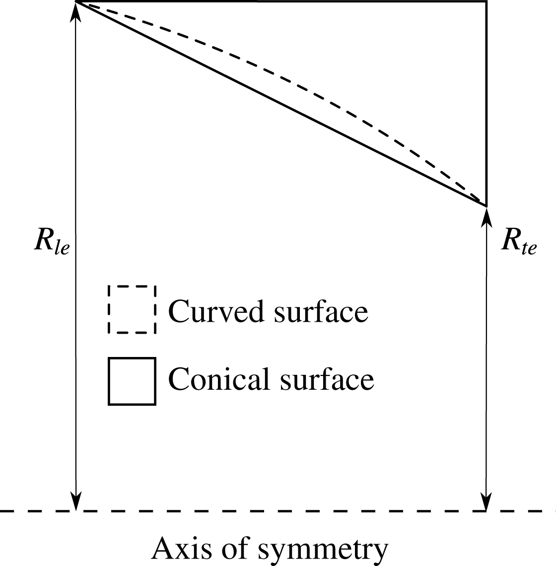
To explore the differences between the flow fields caused by curved and conical internal surfaces, additional numerical and experimental tests were completed. A conical model was created such as that in figure 15, where the leading-edge radius,
 $R_{le}$
, and the trailing-edge radius,
 $R_{te}$
, were the same as those generated by the
 $\unicode[STIX]{x1D6FC}=8^{\circ },R_{c}=1.5,L_{w}=0.5$
model. The conical surface then joined the leading and trailing edge, creating parameters where
 $\unicode[STIX]{x1D6FC}=18.1^{\circ }$
and
 $R_{c}=\infty$
. No flow plane curvature would then be imposed on the shock wave, as the internal surface is straight, but transverse curvature would still be present due to the ring wedge model’s axisymmetric nature.
Conical and curved internal ring wedge surface.

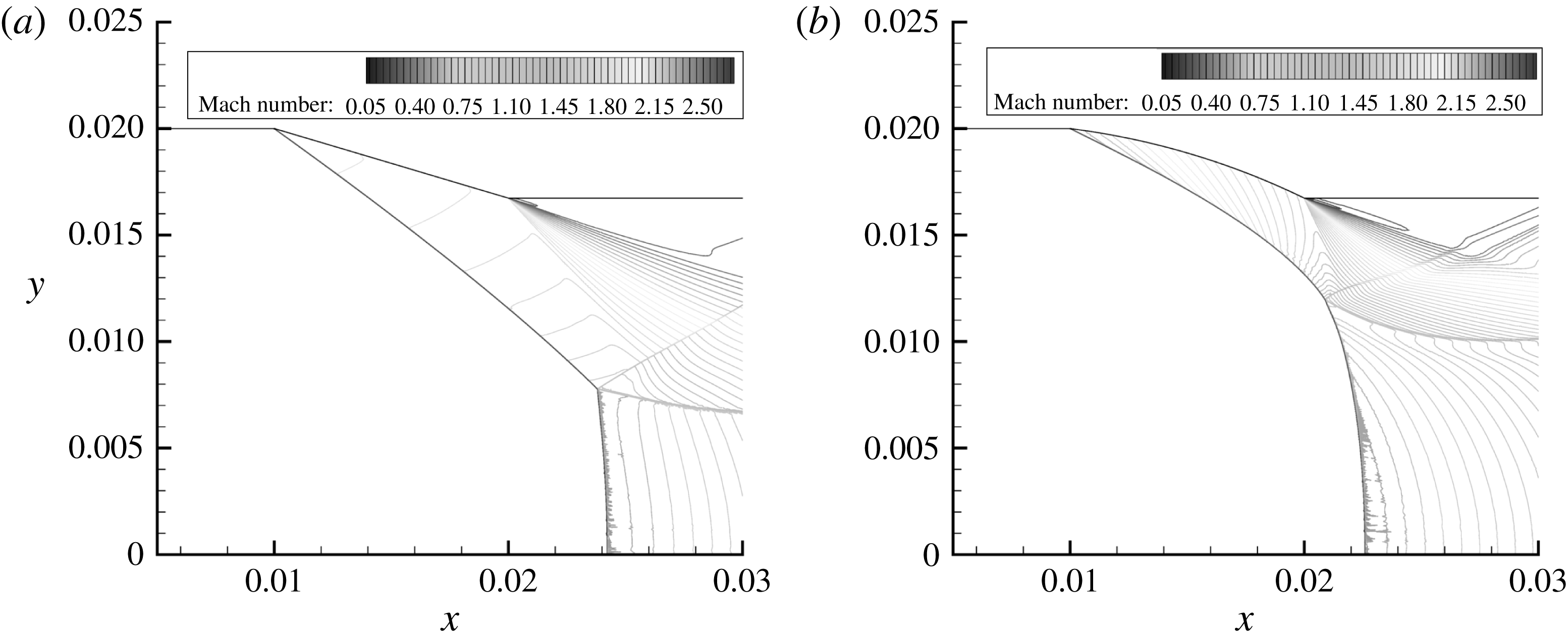
Figure 16 displays the Mach number contour plots for the
 $\unicode[STIX]{x1D6FC}=18.1^{\circ },R_{c}=\infty$
and
 $\unicode[STIX]{x1D6FC}=8^{\circ },R_{c}=1.5$
models at Mach 2.7. The resulting flow fields in either case are very different. Firstly, in figure 16(a), although the internal surface is conical a Mach number variation exists between the attached initial shock wave and the internal surface. This exists due to the transverse curvature that is present, which slightly curves the initial shock wave, increasing the shock angle and thereby reducing the post-shock Mach number. The influence of the transverse curvature is known to increase as the distance to the axis of symmetry decreases. This can be seen in figure 16(a), as the spacing between Mach number contours decreases on approach to the triple point, meaning the shock angle is increasing with progression along the shock wave.
Numerical Mach number contour results. (a)
 $\unicode[STIX]{x1D6FC}=18.1^{\circ },R_{c}=\infty$
model at Mach 2.7; (b)
 $\unicode[STIX]{x1D6FC}=8^{\circ },R_{c}=1.5$
model at Mach 2.7.

Since nothing is interfering with the initial shock wave, due to the supersonic flow’s nature inhibiting pressure waves to travel upstream and the current location of the triple point, transverse curvature must be the only influence. In figure 16(b) the leading and trailing edge are now joined by a curved surface, and so compression waves readjust the flow to its presence and curve the shock wave. A large Mach reflection is present; however, the reflected triple-point shock wave is very weak in comparison to that in figure 16(a), but a clear kink in the shock wave is present after the curved shock segment. Since this weak shock reflection stage exists it could point to a transition region for the shock’s geometry. During this point the shock wave could shift from being continuously curved from the leading edge to the axis of symmetry to developing a kink and Mach reflection. This transition region would occur between very small Mach number increments near Mach 2.7 and would be very difficult to produce experimentally. With the Mach reflection forming further upstream in figure 16(b) than in 16(a) due to the increased shock angle at the triple point, the height of the Mach stem is increased. The increased height promotes its tendency to curve to a larger extent in comparison to the Mach stem produced in the conical case.
Comparing the orientation of the expansion fans in figure 16(a,b) it is evident that the internal surface curvature plays a considerable role in their size and direction. For the conical case the corner reflex angle between the internal surface and the trailing-edge wake is smaller than the reflex angle in the curved internal surface case. This means the strength of the expansion fan is decreased, as the flow has to navigate less of an expansion. The Mach number of the flow at the trailing edge of the curved internal surface is Mach 1.54, which is less than that of the conical case, where it is Mach 1.78 when extracted from numerical results. This is due to the internal curvature continually deflecting the flow. Even though the curved surface’s leading-edge post-shock Mach number is higher, it is continually decreased as the flow is compressed along the surface. The Mach number along the conical surface does not vary to such an extent. As previously mentioned, this causes the leading Mach line of the expansion to form at a steeper angle, which results in the influence of the expansion fan to be felt further upstream. The expansion fan in figure 16(b) covers a larger region and is steeper than that in figure 16(a).
Monochromatic schlieren results for the
 $\unicode[STIX]{x1D6FC}=18.1^{\circ },R_{c}=\infty$
and
 $\unicode[STIX]{x1D6FC}=8^{\circ },R_{c}=1.5$
models are shown in figure 17(a) and 17(b), respectively, at Mach 3.4. Although colour mask schlieren results were obtained under the same conditions, monochromatic results have been displayed instead. The reasoning for the switch being that differences between the two cases are more apparent using monochromatic schlieren. This was particularly the case behind the Mach disk and regions before the initial shock wave. Regarding the impact of the upstream flow quality in figure 17, density gradients are seen ahead of the leading edge. These gradients, however, are caused by the turbulence being captured in the boundary layer on the wind tunnel test section windows. The sensitivity of the schlieren set-up that was used was quite strong, as shown by the extremely dark region of the lower reflection. This increased sensitivity then captured the turbulence which would not have been seen in a flow visualisation schlieren set-up with lower sensitivity or longer exposure time, where the features would blur into a smoother background.
Monochromatic schlieren results. (a)
 $\unicode[STIX]{x1D6FC}=18.1^{\circ },R_{c}=\infty$
model at Mach 3.4; (b)
 $\unicode[STIX]{x1D6FC}=8^{\circ },R_{c}=1.5$
model at Mach 3.4.

With the Mach number being increased to Mach 3.4 in figure 17(a), the transverse-curvature-induced concavity of the shock wave can be more easily noticed. Similarly, in figure 17(b), the expansion-fan-induced convexity in the initial shock wave is recognisable to what has been seen in previous models, now that the Mach reflection triple point has moved further downstream. The banded presence of the upper expansion fan can be seen in the post-shock flow field with its direction orientated towards the initial shock wave. The axial symmetry of the flow fields is what generates the dark patch ahead of the upper initial shock wave in each case as the shock surface rotates around the axis of symmetry. This dark patch, formed by the light blocked by the horizontal knife edge, is more uniform in figure 17(a) than in figure 17(b). This could be as a result of the expansion-fan-induced shock wave convexity interfering with the concave curvature of the initial shock wave in figure 17(b) as one progresses along its length. In figure 17(a) the shock wave is only curved due to transverse curvature, as the expansion fan is seen to be angled further downstream. The lack of conflicting curvature sources then allows a more uniform density gradient to form.
Although the Mach disks in figure 17(a,b) are of the same relative size, they produce considerably different density gradients in their exhausts. Therefore, they must possess an axially symmetric difference in curvature. Seeing as there is a difference in the initial shock wave that forms the Mach reflection in either case, one being more concave and the other more convex, the conditions that form the reflection might differ. As a result, the formation of the Mach disk and triple-point slip layer might not be identical.
5 Conclusions
For the highest curvature case, the rotating of the compression waves occurred to such an extent that with the influencing flow plane and transverse curvature they began to bend inwards. As a result an initial reflection formed before the main Mach reflection, creating an initial slip layer and reflected shock that dissipated in strength with Mach number progression.
With increasing internal surface curvature, the trailing-edge corner angle, around which the expansion fan rotates the flow, increases. This causes the strength and pressure ratio across the expansion to increase, changing its direction and influence on downstream shock structures.
The strength of the initial shock wave was shown to increase for increased internal surface curvatures due to it becoming steeper. This resulted in the Mach reflection forming closer to the trailing edge, reducing the impact of transverse curvature due to the influence of the expansion fan.
With
 $\unicode[STIX]{x1D6FC}$
increasing from a flow tangent scenario to a non-zero value, the flow dynamics at the leading edge change from an isentropic compression to an attached leading-edge shock wave. This steepens the initial shock angle, increasing the size of the Mach disk.
The net flow deflection between the leading and trailing edge remains constant but the post-shock flow is slowed more greatly as
 $\unicode[STIX]{x1D6FC}$
increases. This steepens the angle of the compression waves and causes the leading-edge shock to be curved to a greater extent.
The corner angle is affected with variation in
 $\unicode[STIX]{x1D6FC}$
as the angle between the back trailing-edge surface and internal surface trailing edge’s tangent changes. As a result the expansion fan strength is influenced by the same means as varying the internal surface curvature, affecting the downstream shock structure and flow conditions. The strengths of the initial and reflected Mach reflection shocks were seen to vary with changing
 $\unicode[STIX]{x1D6FC}$
, as it controlled the direction and curvature applied to the leading-edge curved shock wave segment.
Since the trailing edge of the conical model’s corner experienced a smaller corner angle and faster wall-bounded flow, the influence of the expansion fan was directed downstream and not towards the initial shock wave. This allowed the effects of transverse curvature to be more effectively visualised concerning the shock shape and Mach number variation.
Large differences were noted in the flow field produced by both cases due to the imposed curvature involved, changing the shock angle for the curved model. The transverse curvature applied in the conical case produced more uniform pre-shock axially symmetric density gradients due to the lack of conflicting expansion-wave-induced convexity.