1 Introduction
Electrospraying is a technique for atomizing liquids into charged droplets. In its most common and simplest configuration, the liquid is continuously fed to the tip of a capillary tube or needle, while applying a sufficiently high voltage difference with respect to a ground electrode. Several distinct atomization modes may occur depending on the strength of the electric field and the physical properties and flow rate of the fluid (Cloupeau & Prunet-Foch Reference Cloupeau and Prunet-Foch1989; Grace & Marijnissen Reference Grace and Marijnissen1994; Jaworek & Krupa Reference Jaworek and Krupa1999; Marginean, Nemes & Vertes Reference Marginean, Nemes and Vertes2007; Verdoold et al. Reference Verdoold, Agostinho, Yurteri and Marijnissen2014), among which the cone–jet mode has attracted the most attention from researchers. In this mode, the balance between capillary and electrostatic forces on the surface of the fluid results in a conical meniscus (Taylor Reference Taylor1964) that issues a long jet from its cusp. The jet eventually breaks up into charged droplets by capillary or Rayleigh instabilities. The interest in this atomization mode resides in its steadiness, the narrow diameter distribution of the droplets, and the smallness of the diameters of the jet and droplets that are achievable (down to a few nanometres).
The seminal work of Loscertales et al. (Reference Loscertales, Barrero, Guerrero, Cortijo, Marquez and Gañán-Calvo2002) demonstrated the coaxial electrospraying technique, an extension of the cone–jet mode, as a method for producing compound jets and droplets of immiscible liquids at the micro/nanoscale. The coaxial electrospraying technique has been used to produce fibres, usually using liquid precursors of very high viscosity to help extend the stability and associated length of the jet. Downstream treatment with physicochemical processes render the final fibre (Moghe & Gupta Reference Moghe and Gupta2008; Lu, Wang & Wei Reference Lu, Wang and Wei2009). Often the fibre precursors are dissolved polymers, the liquids exhibit viscoelastic features, and the coaxial electrospraying technique for producing fibres can be regarded as a variant of the electrospinning technique. Compound fibres produced in this way have attracted interest in materials science (Li & Xia (Reference Li and Xia2004), Chen et al. (Reference Chen, Wang, Di, Zhao, Song and Jiang2010), Qu, Wei & Guo (Reference Qu, Wei and Guo2013), and references therein) and pharmacology (He, Huang & Han Reference He, Huang and Han2009; Ji et al. Reference Ji, Yang, Wang, Mao, Guo, Xiao and He2013; Zamani, Prabhakaran & Ramakrishna Reference Zamani, Prabhakaran and Ramakrishna2013). Encapsulated droplets, core–shells, and hollow and porous particles have also been produced with the coaxial electrospraying technique. The advantages of this technique include: encapsulation rates of nearly 100 %; good control of the core–shell geometry; and the gentle injection of the core, which allows the preservation of fragile mixtures (e.g. the bioactivity of some therapeutic agents is prone to denaturation under more energetic conditions). Coaxial electrospraying has been successfully used for the production of fast-dissolving core–shell composite microparticles (Li et al. Reference Li, Yu, Williams and Wang2014), protein-encapsulated particles (Xu & Hanna Reference Xu and Hanna2006) and cocoa butter microcapsules (Bocanegra et al. Reference Bocanegra, Gaonkar, Barrero, Loscertales, Pechack and Marquez2005; Gómez-Mascaraque et al. Reference Gómez-Mascaraque, Tordera, Fabra, Martínez-Sanz and Lopez-Rubio2019). Zhang et al. (Reference Zhang, Huang, Si and Xu2012) and Zamani et al. (Reference Zamani, Prabhakaran and Ramakrishna2013) provide extensive reviews of the applications of coaxial electrospraying.
1.1 Cone–jet electrohydrodynamics background
Extensive reviews of the physics of cone–jets can be found, among others, in Fernández de la Mora (Reference Fernández de la Mora2007), Gañán-Calvo et al. (Reference Gañán-Calvo, López-Herrera, Herrada, Ramos and Montanero2018) and Rosell-Llompart, Grifoll & Loscertales (Reference Rosell-Llompart, Grifoll and Loscertales2018). The cone–jet of a single fluid can be sustained within ranges of the emitter voltage and flow rate that depend on the physical properties of the fluid and the imposed geometry (emitter size, its distance to the electrode, geometry of the electrode, etc.). Once the appropriate voltage range is set, in this regime properties such as the diameter of the jet and the electrical current are, to a great extent, independent of the geometry and the potential of the electrodes (Fernandez de la Mora & Loscertales Reference Fernandez de la Mora and Loscertales1994; Herrada et al. Reference Herrada, Lopez-Herrera, Gañan-Calvo, Vega, Montanero and Popinet2012; Ponce-Torres et al. Reference Ponce-Torres, Rebollo-Muñoz, Herrada, Gañán-Calvo and Montanero2018). These experimental observations are consequences of the local nature of this problem, which is dominated by processes occurring within the small region in which the cone transitions into the jet. These processes can be analysed using the natural scales of the problem for moderate to low viscosities:  $d_{e}=(\unicode[STIX]{x1D6FE}\unicode[STIX]{x1D700}_{a}^{2}/\unicode[STIX]{x1D70C}\unicode[STIX]{x1D705}^{2})^{1/3}$,
 $t_{e}=\unicode[STIX]{x1D700}_{a}/\unicode[STIX]{x1D705}$ and
 $p_{e}=(\unicode[STIX]{x1D70C}\unicode[STIX]{x1D705}^{2}\unicode[STIX]{x1D6FE}^{2}/\unicode[STIX]{x1D700}_{a}^{2})^{1/3}$ for length, time and pressure, where
 $\unicode[STIX]{x1D70C}$,
 $\unicode[STIX]{x1D6FE}$,
 $\unicode[STIX]{x1D705}$ and
 $\unicode[STIX]{x1D700}_{a}$ are the liquid density, surface tension, electrical conductivity and vacuum permittivity, respectively.
The locality of the problem appears immediately, as in the vast majority of cases  $d_{e}$ is much smaller than the scale of the feeding tube
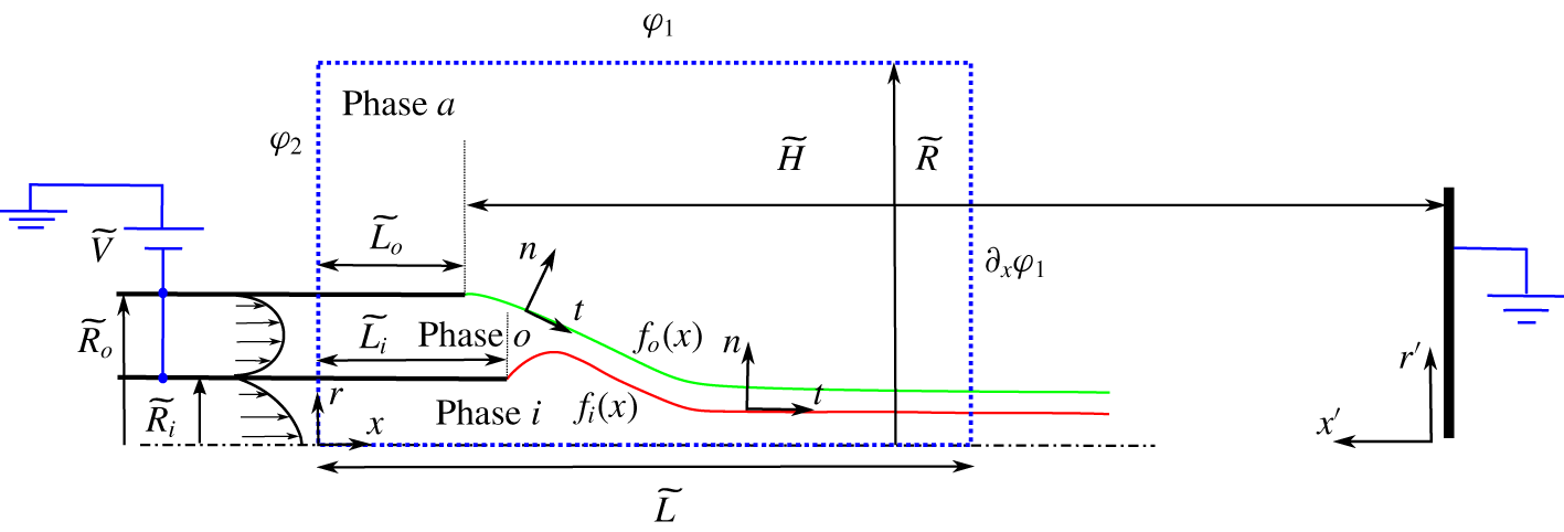
 $\widetilde{R}_{o}$ (figure 1), justifying the use of the electrostatic field of a Taylor cone (Taylor Reference Taylor1964) as the base solution instead of that corresponding to any particular electrode geometry (Pantano, Gañán-Calvo & Barrero Reference Pantano, Gañán-Calvo and Barrero1994). By doing this, semi-analytical (Gañán-Calvo Reference Gañán-Calvo1997, Reference Gañán-Calvo1999) and numerical (Higuera Reference Higuera2003; Gamero-Castaño & Magnani Reference Gamero-Castaño and Magnani2019) models of cone–jets have taken advantage of that local nature to obtain a universal solution and scaling laws for key observables such as the current,
 $I\sim (\unicode[STIX]{x1D6FE}\unicode[STIX]{x1D705}Q)^{1/2}$, and the radius of the base of the jet and the droplets,
 $r_{G}=(\unicode[STIX]{x1D70C}\unicode[STIX]{x1D700}_{a}Q^{3}/\unicode[STIX]{x1D6FE}\unicode[STIX]{x1D705})^{1/6}$ (Gañán-Calvo, Dávila & Barrero Reference Gañán-Calvo, Dávila and Barrero1997; Gañán-Calvo Reference Gañán-Calvo2004; Gañán-Calvo & Montanero Reference Gañán-Calvo and Montanero2009); here
 $Q$ and
 $\unicode[STIX]{x1D6FD}$ stand for the flow rate and fluid relative permittivity, respectively.
Sketch of the problem. The (blue) dashed rectangle indicates the computational domain.

A liquid in contact with an electrode and exposing a free surface to an immiscible environment in static conditions, such as the ideal case proposed by Taylor (Reference Taylor1964), is characterized by an equipotential interface, charge neutrality in the bulk and zero inner electric field. Additional features include the absence of inner electric stress and full relaxation of the charge on the surface (even in the presence of an applied external field). If a dynamic cone–jet develops because the applied field overcomes a critical value, some of these ideal characteristics change. In particular, the intense advection of interfacial charge taking place in the cone-to-jet transition region prevents the surface from remaining equipotential and electric fields develop inside the liquid, while the bulk remains free of charges. This situation has been frequently modelled with the leaky dielectric model (LDM) of Melcher & Taylor (Reference Melcher and Taylor1969), in which electrical forces acting on the liquid and net charge are circumscribed to the interface, while the bulk acts as an electrically neutral reservoir through which charge is transported by ohmic conduction. The surface charge density is determined by surface advection and the injection or withdrawal of charge by ohmic conduction from the bulk. Some authors include surface conduction effects (Burcham & Saville Reference Burcham and Saville2002; Burton & Taborek Reference Burton and Taborek2011) with an independent value of a surface conductivity as an intelligent integral approximation to having very different concentrations of ionic species in the surface charge layer and in the bulk, resulting in different ensemble values of the conductivity (Saville Reference Saville1997). This results in an augmented version of the charge conservation at the surface. In this work we neglect surface conduction effects in the ample limit subsequently discussed. The ratio between the electric relaxation time and the characteristic hydrodynamic time,  $t_{e}/t_{h}$, measures the relative contribution of the two transport mechanisms, and is indicative of how far the surface charge is from its natural relaxed state. For example, the surface charge is relaxed and the equipotential limit is recovered in the limit
 $t_{e}/t_{h}\rightarrow 0$.
The LDM is often seen as the constitutive equations of the electrohydrodynamic (EHD) phenomena, instead of a powerful and successful approximation of the general electrokinetic phenomena behind it. Since the pioneering work of Saville (Reference Saville1997), a number of investigations have attempted to clarify the connection and explored the circumstances under which the LDM is supported by electrokinetics (Zholkovskij, Masliyah & Czarnecki Reference Zholkovskij, Masliyah and Czarnecki2002; Schnitzer & Yariv Reference Schnitzer and Yariv2015; Mori & Young Reference Mori and Young2018). Requisites for using the LDM are the existence of a Debye length much smaller than the characteristic length of the problem, and of an electric field across the Debye layer low enough to preserve its structure (Schnitzer & Yariv Reference Schnitzer and Yariv2015). Recently, Mori & Young (Reference Mori and Young2018) have shown that if  $t_{e}/t_{h}\gtrsim 1$ the bulk cannot be regarded as a neutral reservoir of charge, compromising the validity of the LDM.
In the majority of conditions for sufficiently large flow rates, electrosprays are perfectly described by the LDM (Gañán-Calvo Reference Gañán-Calvo1999; Gañán-Calvo et al. Reference Gañán-Calvo, López-Herrera, Herrada, Ramos and Montanero2018), because the above requisites are fulfilled. Recently, Ponce-Torres et al. (Reference Ponce-Torres, Rebollo-Muñoz, Herrada, Gañán-Calvo and Montanero2018) have studied the minimum flow rate limit in electrosprays by performing a rigorous linear stability analysis of the steady solution. They showed that, in general, what Gañán-Calvo (Reference Gañán-Calvo1999) and subsequent works postulated linking the minimum flow rate to having hydrodynamic times comparable to  $t_{e}$ is supported by the global stability analysis of a Taylor cone–jet.
The physics of coaxial electrosprays is not so well understood as the single-phase electrospray counterpart. Loscertales et al. (Reference Loscertales, Barrero, Guerrero, Cortijo, Marquez and Gañán-Calvo2002) introduced the concept of ‘driving liquid’ as the one on which the EHD forces act. This concept applies to pairs of liquids with disparate electric relaxation times. Their experiments show that the  $Q^{1/2}$ law for the current also applies to coaxial electrosprays, where the flow rate is that of the driving liquid. López-Herrera et al. (Reference López-Herrera, Barrero, López, Loscertales and Márquez2003) discuss in more depth the concept of driving liquid and formulate scaling laws based those of cone–jets of single liquids. Chen et al. (Reference Chen, Jia, Yin, Cheng and Lu2005) describe different modes present in coaxial electrospraying and postulate the homogeneity of internal and external velocities in the jet. Mei & Chen (Reference Mei and Chen2007) focus on the encapsulation process; in particular, they explore the influence of physical parameters in the morphology of the capsules. They experiment with several inner fluids while always using an oil of very low conductivity and permittivity as the outer fluid, i.e. the driving fluid is always the inner one. Their experiments confirm some of the findings of Loscertales et al. (Reference Loscertales, Barrero, Guerrero, Cortijo, Marquez and Gañán-Calvo2002) and López-Herrera et al. (Reference López-Herrera, Barrero, López, Loscertales and Márquez2003), such as the monodispersity of the sprays, and the
 $I\sim Q^{1/2}$ dependence or the linear dependence of the size of the capsule with the inner flow rate at low flow rates; they also report new trends such as the independence of capsule size on the flow rate for large
 $Q$, and map the conditions for controllable encapsulation. Finally, Mei & Chen (Reference Mei and Chen2007, Reference Mei and Chen2008) argue that stable coaxial electrosprays require both that the permittivity of the outer fluid is lower than that of the inner fluid, and that the surface tensions meet the static stability criteria of Torza & Mason (Reference Torza and Mason1970).
The present work is the first numerical simulation of coaxial electrosprays. The simulation by Xu et al. (Reference Xu, Qin, Yin, Hua, Pack and Wang2013) using a commercial code is for inner and outer fluids that have different solute concentrations but are otherwise identical, i.e. it is for miscible fluids. The one-dimensional (1-D) simulation by Higuera (Reference Higuera2007) is characterized by a low electric field and high flow rate, i.e. it deals with a coaxial jet rather than a coaxial cone–jet; furthermore, the core fluid is a perfect dielectric. The method in the present article is based on the mapping of three distinct subdomains (inner and outer electrosprayed liquids, and surrounding atmosphere) into three fixed domains through coordinate transformations. The equations are spatially discretized with the Chebyshev spectral collocation technique in the radial direction and uniformly in the axial direction. The resulting system of nonlinear algebraic equations is solved with the iterative Newton–Raphson technique, with a Jacobian that is efficiently calculated by using symbolic functions derived previously. The method was first proposed by Herrada et al. (Reference Herrada, Lopez-Herrera, Gañan-Calvo, Vega, Montanero and Popinet2012), improved by Herrada & Montanero (Reference Herrada and Montanero2016), and has been successfully applied to other capillary problems (Ponce-Torres, Vega & Montanero Reference Ponce-Torres, Vega and Montanero2016; Cruz-Mazo et al. Reference Cruz-Mazo, Herrada, Gañán-Calvo and Montanero2017; Ponce-Torres et al. Reference Ponce-Torres, Montanero, Herrada and Vega2017).
In this work we use the LDM to reproduce the dynamics of the coaxial electrospray (Melcher & Taylor Reference Melcher and Taylor1969; Saville Reference Saville1997), which implies that the smallest hydrodynamic time scale of the process should be at most comparable to the largest charge relaxation time. Furthermore, we are only interested in the axisymmetric and steady-state solution, which limits the imposed liquid flow rates to those ranges for which the system is stable. Since in this work we do not attempt to analyse the global stability of the system, we should resort to experiments as an initial guide to perform the first numerical two-dimensional (2-D) axisymmetric studies of coaxial electrosprays, and report the most important physical features found.
2 Formulation of the problem
Figure 1 shows schematically the configuration considered in this work. A metallic capillary tube of radius  $R_{i}$ is inserted concentrically into a second tube of radius
 $R_{o}$. Both tubes are held at constant voltage
 $V$ with respect to a planar grounded electrode located at a distance
 $H$. The tubes have negligible thickness. The inner and outer liquids are injected with flow rates
 $Q_{i}$ and
 $Q_{o}$, respectively, and are immiscible. The free surface separating the inner and outer liquids,
 $r=f_{i}(x)$, has an interfacial surface tension
 $\unicode[STIX]{x1D6FE}_{i}$, while the outer free surface
 $r=f_{o}(x)$ separating the outer liquid and the surrounding atmosphere has a surface tension
 $\unicode[STIX]{x1D6FE}_{o}$. We use the subindex
 $i$ to denote physical properties and variables associated with the inner liquid and the inner free surface, the subindex
 $o$ for the outer fluid and outer free surface, and the subindex
 $a$ for the surrounding atmosphere. The density and viscosity of the surrounding atmosphere are sufficiently low to dismiss any dynamical effect on the solution.
The equations are made dimensionless with the group  $\{\unicode[STIX]{x1D70C}_{i},\unicode[STIX]{x1D705}_{i},\unicode[STIX]{x1D6FE}_{o},\unicode[STIX]{x1D700}_{a}\}$. The fundamental magnitudes resulting from this choice are
 $$\begin{eqnarray}d_{e}=\left(\frac{\unicode[STIX]{x1D6FE}_{o}\unicode[STIX]{x1D700}_{a}^{2}}{\unicode[STIX]{x1D70C}_{i}\unicode[STIX]{x1D705}_{i}^{2}}\right)^{1/3},\quad m_{e}=\frac{\unicode[STIX]{x1D6FE}_{o}\unicode[STIX]{x1D700}_{a}^{2}}{\unicode[STIX]{x1D705}_{i}^{2}},\quad t_{e}=\frac{\unicode[STIX]{x1D700}_{a}}{\unicode[STIX]{x1D705}_{i}}\quad \text{and}\quad I_{e}=\left(\frac{\unicode[STIX]{x1D6FE}_{o}^{2}\unicode[STIX]{x1D700}_{a}}{\unicode[STIX]{x1D70C}_{i}}\right)^{1/2},\end{eqnarray}$$
where  $d_{e}$,
 $m_{e}$,
 $t_{e}$ and
 $I_{e}$ denote the reference length, mass, time and electrical current, respectively. Henceforth, symbols capped with a tilde will denote dimensional variables, while uncapped symbols are reserved for dimensionless variables.
The dependent variables of the model are: the velocity vector, pressure and electric potential field in the inner liquid,  $\boldsymbol{v}_{\boldsymbol{i}}$,
 $p_{i}$ and
 $\unicode[STIX]{x1D719}_{i}$; those in the outer liquid,
 $\boldsymbol{v}_{\boldsymbol{o}}$,
 $p_{o}$ and
 $\unicode[STIX]{x1D719}_{o}$; the electric potential in the surrounding atmosphere,
 $\unicode[STIX]{x1D719}_{a}$; the positions of the two free surfaces,
 $f_{i}$ and
 $f_{o}$; and the surface charge in the free surfaces,
 $\unicode[STIX]{x1D70E}_{i}$ and
 $\unicode[STIX]{x1D70E}_{o}$. It is worth noting that a key contribution of this work to enlighten the physics of coaxial electrospray is the identification and evaluation of the surface charge at the inner free surface, whose existence, nature and quantification is here theoretically determined for a general 2-D axisymmetric configuration for the first time, while it was also studied in Higuera (Reference Higuera2007) using a 1-D approximation. In physical terms, what sustains the existence of that inner surface charge is the differences in the electrical conductivities and relaxation times of both inner and outer domains: what we have learned in the process of this study is that, in the absence of that surface charge, no global charge flow balance would be possible.
The equations for the velocity vector, pressure and electric potential fields in subdomain  $k$ are
 $$\begin{eqnarray}\displaystyle & \unicode[STIX]{x1D735}\boldsymbol{\cdot }\boldsymbol{v}_{k}=0, & \displaystyle\end{eqnarray}$$
 $$\begin{eqnarray}\displaystyle & \displaystyle \unicode[STIX]{x1D70C}_{k}^{r}\boldsymbol{v}_{k}\boldsymbol{\cdot }\unicode[STIX]{x1D735}\boldsymbol{v}_{k}=-\unicode[STIX]{x1D735}p_{k}+\frac{1}{Re_{k}}\unicode[STIX]{x1D6FB}^{2}\boldsymbol{v}_{k} & \displaystyle\end{eqnarray}$$
and
 $$\begin{eqnarray}\unicode[STIX]{x1D6FB}^{2}\unicode[STIX]{x1D719}_{k}=0,\end{eqnarray}$$
where  $Re_{k}=(\unicode[STIX]{x1D6FE}_{o}^{2}\unicode[STIX]{x1D70C}_{i}\unicode[STIX]{x1D700}_{a}/\unicode[STIX]{x1D705}_{i}\unicode[STIX]{x1D707}_{k}^{3})^{1/3}$ is the Reynolds number in subdomain
 $k$, and
 $\unicode[STIX]{x1D70C}_{k}^{r}$ is the relative density, with values
 $\unicode[STIX]{x1D70C}_{i}^{r}=1$ and
 $\unicode[STIX]{x1D70C}_{o}^{r}=\unicode[STIX]{x1D70C}_{o}/\unicode[STIX]{x1D70C}_{i}$.
The constraints at the free surface  $k$ include the balance of stresses along the normal
 $\boldsymbol{n}_{k}$ and tangential
 $\boldsymbol{t}_{k}$ directions, the kinematic velocity condition, conservation of charge, and the condition for the jump of the normal components of the electric field
 $E_{n}$ across the interface:
 $$\begin{eqnarray}\displaystyle & \Vert p\Vert _{k}-\unicode[STIX]{x1D6FE}_{k}^{r}\unicode[STIX]{x1D735}\boldsymbol{\cdot }\boldsymbol{n}_{k}+\boldsymbol{n}_{k}\boldsymbol{\cdot }\Vert \unicode[STIX]{x1D70F}_{v}+\unicode[STIX]{x1D70F}_{e}\Vert _{k}\boldsymbol{\cdot }\boldsymbol{n}_{k}=0, & \displaystyle\end{eqnarray}$$
 $$\begin{eqnarray}\displaystyle & \boldsymbol{t}_{k}\boldsymbol{\cdot }\Vert \unicode[STIX]{x1D70F}_{v}+\unicode[STIX]{x1D70F}_{e}\Vert _{k}\boldsymbol{\cdot }\boldsymbol{n}_{k}=0, & \displaystyle\end{eqnarray}$$
 $$\begin{eqnarray}\displaystyle & \boldsymbol{v}_{k}\boldsymbol{\cdot }\boldsymbol{n}_{k}=0, & \displaystyle\end{eqnarray}$$
 $$\begin{eqnarray}\displaystyle & \unicode[STIX]{x1D735}_{s}(\boldsymbol{v}_{s},_{k}\unicode[STIX]{x1D70E}_{k})=\Vert \unicode[STIX]{x1D705}E_{n}\Vert _{k}, & \displaystyle\end{eqnarray}$$
 $$\begin{eqnarray}\displaystyle & \unicode[STIX]{x1D70E}_{k}=\Vert \unicode[STIX]{x1D6FD}E_{n}\Vert _{k}. & \displaystyle\end{eqnarray}$$
Here  $\Vert X\Vert _{k}$ stands for the jump of the quantity
 $X$ across the interface, e.g.
 $\Vert X\Vert _{i}=X_{o}-X_{i}$;
 $\unicode[STIX]{x1D735}_{s}$ is the gradient along the surface;
 $\boldsymbol{v}_{s}$ is the velocity at the surface;
 $\unicode[STIX]{x1D70E}$ is the surface charge density; and
 $\unicode[STIX]{x1D6FE}_{k}^{r}$ is the relative surface tension, with values
 $\unicode[STIX]{x1D6FE}_{i}^{r}=\unicode[STIX]{x1D6FE}_{i}/\unicode[STIX]{x1D6FE}_{o}$ and
 $\unicode[STIX]{x1D6FE}_{o}^{r}=1$. Here, we can safely neglect surface conductivity effects as long as the Debye length
 $\unicode[STIX]{x1D706}$ is smaller than
 $d_{e}E_{n,k}/E_{t,k}$, which is true in ample conditions where the diffusivity
 $D_{k}$ of the ionic species in the liquid is sufficiently small compared to
 $d_{e}^{2}/t_{e}(E_{n,k}/E_{t,k})^{2}$ (Gañán-Calvo et al. Reference Gañán-Calvo, López-Herrera, Herrada, Ramos and Montanero2018). Furthermore,
 $\unicode[STIX]{x1D70F}_{v}$ and
 $\unicode[STIX]{x1D70F}_{e}$ are the viscous and electrostatic stress tensors defined in the three subdomains by
 $$\begin{eqnarray}\unicode[STIX]{x1D70F}_{v,k}=\frac{1}{Re_{k}}\left(\begin{array}{@{}cc@{}}2\unicode[STIX]{x2202}_{r}u_{k} & \unicode[STIX]{x2202}_{x}u_{k}+\unicode[STIX]{x2202}_{r}w_{k}\\ \unicode[STIX]{x2202}_{x}u_{k}+\unicode[STIX]{x2202}_{r}w_{k} & \unicode[STIX]{x2202}_{x}w_{k}\end{array}\right)\end{eqnarray}$$
and
 $$\begin{eqnarray}\unicode[STIX]{x1D70F}_{e,k}=\frac{\unicode[STIX]{x1D6FD}_{k}}{2}\left(\begin{array}{@{}cc@{}}E_{n,k}^{2} & 2E_{n,k}E_{t,k}\\ 2E_{n,k}E_{t,k} & E_{t,k}^{2}\end{array}\right),\end{eqnarray}$$
where  $u_{k}$ and
 $w_{k}$ are the radial and axial components of the velocity in subdomain
 $k$, respectively. Note that the ambient subdomain is dynamically negligible,
 $\unicode[STIX]{x1D70F}_{v,a}=0$. Furthermore, the velocities and potential are continuous at the two free surfaces
 $$\begin{eqnarray}\boldsymbol{v}_{i}=\boldsymbol{v}_{o}|_{(r=f_{i}(x),x)},\quad \unicode[STIX]{x1D719}_{i}=\unicode[STIX]{x1D719}_{o}|_{(r=f_{i}(x),x)},\quad \unicode[STIX]{x1D719}_{o}=\unicode[STIX]{x1D719}_{a}|_{(r=f_{o}(x),x)}.\end{eqnarray}$$
The flow is fully developed upstream in the capillary tubes, resulting in a parabolic velocity profile for the inlet boundary condition and non-slip velocity condition at the wall of the tubes:
 $$\begin{eqnarray}\left.\begin{array}{@{}c@{}}u_{i}(r,x=0)=u_{o}(r,x=0)=0,\quad w_{i}(r,x=0)={\displaystyle \frac{2Q_{i}}{\unicode[STIX]{x03C0}R_{i}^{2}}}\left(1-{\displaystyle \frac{r^{2}}{R_{i}^{2}}}\right),\\ w_{o}(r,x=0)={\displaystyle \frac{2Q_{o}[(R_{i}^{2}-R_{o}^{2})\log (r/R_{i})+(r^{2}-R_{i}^{2})\log (R_{o}/R_{i})]}{\unicode[STIX]{x03C0}(R_{i}^{2}-R_{o}^{2})[(R_{i}^{2}-R_{o}^{2})+(R_{i}^{2}+R_{o}^{2})\log (R_{o}/R_{i})]}}.\end{array}\right\}\end{eqnarray}$$
The simpler expression as  $w_{o}(r,x=0)=[6Q_{o}/\unicode[STIX]{x03C0}(R_{o}^{2}-R_{i}^{2})][(R_{o}-r)/(R_{o}-R_{i})]\times [(r-R_{i})/(R_{o}-R_{i})]$ can be used with sufficient approximation for our purposes, since this condition does not alter in any appreciable way the results given the smallness of the liquid velocities in the tubes compared to those of the recirculation regions and, more importantly, those in the transition region.
The boundary conditions for the electric potential in the surrounding atmosphere are those used by Herrada et al. (Reference Herrada, Lopez-Herrera, Gañan-Calvo, Vega, Montanero and Popinet2012) in their numerical study of a single electrospray. The potential at the top boundary,  $r=R$, has the analytical form derived by Gañán-Calvo et al. (Reference Gañán-Calvo, Lasheras, Dávila and Barrero1994) as
 $$\begin{eqnarray}\unicode[STIX]{x1D711}_{1}(r^{\prime },x^{\prime })=\frac{-K_{v}\unicode[STIX]{x1D6F7}}{\ln (4\widetilde{H}/\widetilde{R}_{o})}\ln \left\{\frac{(H-x^{\prime })+\sqrt{r^{\prime 2}+(H-x^{\prime })^{2}}}{(H+x^{\prime })+\sqrt{r^{\prime 2}+(H+x^{\prime })^{2}}}\right\},\end{eqnarray}$$
where  $(r^{\prime },x^{\prime })$ are the cylindrical coordinates with origin at the intersection of the axis with the ground planar electrode (see figure 1). Equation (2.14) is the field induced by a semi-infinite line of charges, modified to model an equipotential semi-infinite cylinder of finite radius through the introduction of the dimensionless function
 $K_{v}=K_{v}(\widetilde{H}/\widetilde{R}_{o})$. We justify this election of the far boundary condition based on its consistency with the experimental set-up and the good results obtained in previous works (Gañán-Calvo et al. Reference Gañán-Calvo, Lasheras, Dávila and Barrero1994; Herrada et al. Reference Herrada, Lopez-Herrera, Gañan-Calvo, Vega, Montanero and Popinet2012; Ponce-Torres et al. Reference Ponce-Torres, Rebollo-Muñoz, Herrada, Gañán-Calvo and Montanero2018). For consistency as well with that choice, at the right boundary
 $x=L$ we impose the Neumann boundary condition
 $$\begin{eqnarray}\unicode[STIX]{x2202}_{x}\unicode[STIX]{x1D719}_{a}=\unicode[STIX]{x2202}_{x}\unicode[STIX]{x1D711}_{1},\end{eqnarray}$$
while at the left boundary  $x=0$ we employ a logarithmic profile between the value provided by (2.14) at
 $r=R$ and the potential of the emitter
 $\unicode[STIX]{x1D6F7}$ at
 $r=R_{o}$,
 $$\begin{eqnarray}\unicode[STIX]{x1D711}_{2}(r)=\unicode[STIX]{x1D6F7}-(\unicode[STIX]{x1D6F7}-\unicode[STIX]{x1D711}_{1}(H+L_{o},R))\frac{\ln (r/R_{o})}{\ln (R/R_{o})}.\end{eqnarray}$$
This latter condition does not produce any significant limitation to or restriction on the results obtained, as it has been assessed by comparing the results with those using a linear decay between the potential of the emitter  $\unicode[STIX]{x1D6F7}$ and
 $\unicode[STIX]{x1D711}_{1}(H+L_{o},R)$. Finally, we impose soft exit boundary conditions in the jet,
 $$\begin{eqnarray}\unicode[STIX]{x2202}_{x}w_{k}|_{(r,x=L)}=\unicode[STIX]{x2202}_{x}u_{k}|_{(r,x=L)}=\unicode[STIX]{x2202}_{x}\unicode[STIX]{x1D70E}_{k}|_{(r,x=L)}=\unicode[STIX]{x2202}_{x}\,f_{k}|_{x=L}=0,\end{eqnarray}$$
and symmetry conditions at the axis,
 $$\begin{eqnarray}u_{i}(x,0)=\unicode[STIX]{x2202}_{r}w_{i}|_{(r=0,x)}=\unicode[STIX]{x2202}_{r}\unicode[STIX]{x1D719}_{i}|_{(r=0,x)}=0.\end{eqnarray}$$
The solution of the coaxial electrospray described by the model above is a function of the following dimensionless numbers:
(i) The dimensionless flow rates, Reynolds numbers and relative permittivity of both fluids,
 $Q_{i}$, $Q_{o}$, $Re_{i}$, $Re_{o}$, $\unicode[STIX]{x1D6FD}_{i}$ and $\unicode[STIX]{x1D6FD}_{o}$.
(ii) The relative surface tension, density and electrical conductivity of the liquids,
$\unicode[STIX]{x1D6FE}_{r}=\unicode[STIX]{x1D6FE}_{i}/\unicode[STIX]{x1D6FE}_{o}$, $\unicode[STIX]{x1D6FE}_{r}=\unicode[STIX]{x1D70C}_{o}/\unicode[STIX]{x1D70C}_{i}$ and $\unicode[STIX]{x1D705}_{r}=\unicode[STIX]{x1D705}_{o}/\unicode[STIX]{x1D705}_{i}$.(iii) The applied voltage
$\unicode[STIX]{x1D6F7}$ and the electrode geometry, i.e. the needles’ radii and lengths, $R_{i}$, $R_{o}$, $L_{i}$ and $L_{o}$, and the distance to the ground electrode, $H$.(iv) The computational domain given by the rectangle
$L\times R$.


It is worth noting that the universal solution of a cone–jet of a single fluid, i.e. the solution independent of geometric and/or electrostatic parameters resulting from imposing Taylor’s potential as a far-field boundary condition (Gañán-Calvo Reference Gañán-Calvo1997; Higuera Reference Higuera2003; Gamero-Castaño & Magnani Reference Gamero-Castaño and Magnani2019), is a function of only three parameters. In contrast, the solution of the present model contains 17 parameters. Even if the importance of the geometric and/or electrostatic parameters is discounted, nine fluid parameters remain in the model. Therefore, we will have to analyse the effect of a smaller set of parameters expected to be the most important ones, namely the inner and outer flow rates,  $Q_{i}$ and
 $Q_{o}$, and the ratio of conductivities,
 $\unicode[STIX]{x1D705}_{r}$.
3 Numerical scheme
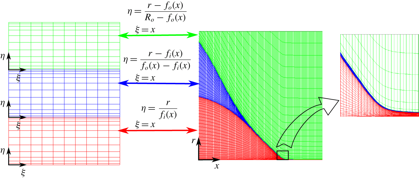
Computational subdomains and grids for the original and mapped variables.

In the numerical scheme, the three subdomains (inner and outer liquids, and the surrounding atmosphere) are mapped into fixed rectangular domains as shown in figure 2. The mapped domains are discretized in the radial  $\unicode[STIX]{x1D702}$ direction with the Chebyshev spectral collocation method, while grid points are uniformly distributed in the axial
 $\unicode[STIX]{x1D709}$ direction. After writing the equations in the
 $\{\unicode[STIX]{x1D709},\unicode[STIX]{x1D702}\}$ variables, the spatial derivatives are discretized with fourth-order accuracy. The program has been built in the computational MATLAB© environment, which facilitates the formulation of the equations in the mapped variables through symbolic calculus. Symbolic calculus simplifies writing the system of nonlinear equations
 $$\begin{eqnarray}{\mathcal{F}}_{q}(u_{1},\ldots ,u_{q},\ldots ,u_{n\times N})=0,\end{eqnarray}$$
where  $u_{q}$ is the
 $q$th unknown,
 $n$ is the total number of unknowns in each grid point and
 $N$ is the total amount of grid points (the total number of unknowns and equations is
 $n\times N$). Furthermore, symbolic calculus enables the exact derivation of the components of the Jacobian,
 $$\begin{eqnarray}{\mathcal{J}}_{pq}=\frac{\unicode[STIX]{x2202}{\mathcal{F}}_{p}}{\unicode[STIX]{x2202}u_{q}},\end{eqnarray}$$
which must be computed to solve the nonlinear system (3.1) with the Newton–Raphson method. The analytical calculation of the Jacobian drastically reduces the cost of its computation with respect to a scheme that evaluates it numerically.
4 Validation
The model has been validated with experiments using deionized water and tributyl phosphate (TBP) as the inner and outer fluids, respectively. The relevant properties of the fluids are shown in table 1. All properties except for the conductivities, which were measured, are taken from Riddick, Bunger & Sakano (Reference Riddick, Bunger and Sakano1986). The surface tension between the two liquids,  $\unicode[STIX]{x1D6FE}_{i}=0.008~\text{N}~\text{m}^{-1}$, is taken from Sagert, Quinn & Lee (Reference Sagert, Quinn and Lee1980). The outer tube is made of stainless steel and has outer and inner diameters of
 $711.2~\unicode[STIX]{x03BC}\text{m}$ and
 $533.4~\unicode[STIX]{x03BC}\text{m}$. The inner fluid is injected through a concentric fused silica tube of outer and inner diameters
 $360~\unicode[STIX]{x03BC}\text{m}$ and
 $200~\unicode[STIX]{x03BC}\text{m}$. The surface of the fused silica tube is metallized, and both tubes are mounted on a stainless-steel T-junction where the emitter potential is applied. A grounded electrode is located downstream at a distance of approximately 1 cm where the droplets are collected and the electrical current is measured with an electrometer. The flow rates of the fluids are controlled independently with syringe pumps (NE-300-US from ArrEssPro Scientific).
Density, viscosity, surface tension, electrical conductivity and relative permittivity, respectively, of the fluid used, given in SI units.

Since the numerical model does not consider the wall thickness of the tubes, we reduce each tube to a cylindrical surface with the mean of their inner and outer radii. The computational domain is kept fixed,  $R/R_{i}=30$,
 $L/R_{i}=12$ and
 $H/R_{i}=40$ (for which
 $K_{v}=0.56$). The lengths of both needles are identical,
 $L_{(o,i)}/R_{i}=1.5$. The axial direction is uniformly discretized with
 $nx=1051$ points, while we use
 $nr_{i}=30$,
 $nr_{o}=20$ and
 $nr_{a}=115$ Chebyshev spectral collocation points in the radial direction, which suffices to obtain a mesh-independent solution.
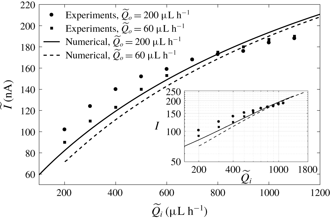
Figure 3 compares the experimental and numerical dimensional electrical current,  $\widetilde{I}$, as a function of the dimensional inner flow rate,
 $\widetilde{Q}_{i}$, for two different outer flow rates,
 $\widetilde{Q}_{o}$ (200 and
 $60~\unicode[STIX]{x03BC}\text{l}~\text{h}^{-1}$). The experimental emitter and simulation potentials are in both cases equal to 4570 V. The maximum discrepancy in the explored range is below 20. Furthermore, as can be observed in the inset in figure 3, the model reproduces the experimental trends:
 $\widetilde{I}$ scales approximately as
 $\widetilde{Q}_{i}^{1/2}$ in the numerical simulations and in the experimental data for
 $\widetilde{Q}_{i}$ below
 $800~\unicode[STIX]{x03BC}\text{l}~\text{h}^{-1}$. Also, a weak dependence on
 $\widetilde{Q}_{o}$ at large values of
 $\widetilde{Q}_{i}$ is observed, which increases monotonically as
 $\widetilde{Q}_{i}$ decreases. The agreement between the experimental and numerical results is good, and justifies the detailed analysis of the model output below.
Dimensional electrical current,  $\widetilde{I}$ (in nA), collected at the grounded electrode as a function of the inner flow rate,
 $\widetilde{Q}_{i}$ (in
 $\unicode[STIX]{x03BC}\text{l}~\text{h}^{-1}$), for different outer flow rates,
 $\widetilde{Q}_{o}$. Symbols and continuous lines correspond to experiments and numerical simulations, respectively. Inner fluid, water; outer fluid, TBP. The inset shows
 $\widetilde{I}$ versus
 $\widetilde{Q}$ in log scale. If data were fitted with potential laws of the form
 $\widetilde{I}\simeq C\widetilde{Q}^{\unicode[STIX]{x1D6FC}}$, then
 $\unicode[STIX]{x1D6FC}$ would be 0.346 and 0.453 for the experimental data with flow rates of 200 and
 $60~\unicode[STIX]{x03BC}\text{l}~\text{h}^{-1}$, respectively, and 0.529 and 0.602 for the numerical data with flow rates of 200 and
 $60~\unicode[STIX]{x03BC}\text{l}~\text{h}^{-1}$, respectively.

5 Results and discussion
Given the large number of free parameters in the model, we restrict the simulations to the geometry described in the validation section (§ 4), and the use of water and TBP as the inner and outer fluids. Only the effects of varying the conductivities and the flow rates of the fluids are studied. Yet, the wealth of physical effects found and the analysis of the critical regions of the system that our model allows justify this monographic report.
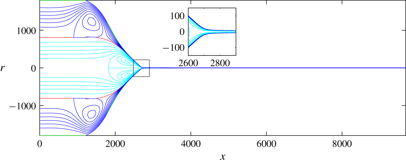
Shape and streamlines of a coaxial electrospray of water in TBP. Here  $Q_{i}=171$ (
 $234~\unicode[STIX]{x03BC}\text{l}~\text{h}^{-1}$),
 $Q_{o}=44$ (
 $60~\unicode[STIX]{x03BC}\text{l}~\text{h}^{-1}$) and
 $\unicode[STIX]{x1D6F7}=197$ (4570 V).

Figure 4 depicts the position of the free surfaces and the streamlines of the flows for a realistic case corresponding to  $\widetilde{Q}_{i}=234~\unicode[STIX]{x03BC}\text{l}~\text{h}^{-1}$,
 $\widetilde{Q}_{o}=60~\unicode[STIX]{x03BC}\text{l}~\text{h}^{-1}$ and
 $\widetilde{\unicode[STIX]{x1D719}}=4570$ V. The values of the dimensionless parameters are
 $Q_{i}=171$,
 $Q_{o}=44$ and
 $\unicode[STIX]{x1D719}=197$. In the scale of figure 4, the outer free surface rapidly approaches the inner one due to the penetration of the electric field through the outer fluid and its ability to shape the inner interface into a Taylor-cone-like meniscus; the outer surface must then approach the inner one due to the high tangential stresses and velocities, and small outer flow rate. Interestingly, a large fraction of the domain of each liquid is occupied by a recirculation region, caused by the strong tangential stresses and associated velocities at the free surfaces, and the need to maintain mass conservation. These recirculation regions occur upstream in the largely static conical region. They provide a way to accommodate the inlet flow condition to the flow in the cone-to-jet transitions and, despite their interesting geometric patterns, have little effect on the key processes of the problem, which are located in the much smaller transition region.
5.1 The transition region
We describe now the main characteristics of the solution in the transition region between cone and jet, for the same electrospraying parameters as in figure 4 ( $Q_{i}=171$,
 $Q_{o}=44$,
 $\unicode[STIX]{x1D719}=197$,
 $\unicode[STIX]{x1D705}_{r}=0.137$,
 $\unicode[STIX]{x1D70C}_{r}=0.976$,
 $\unicode[STIX]{x1D6FE}_{r}=0.29$,
 $Re_{i}=2.18$ and
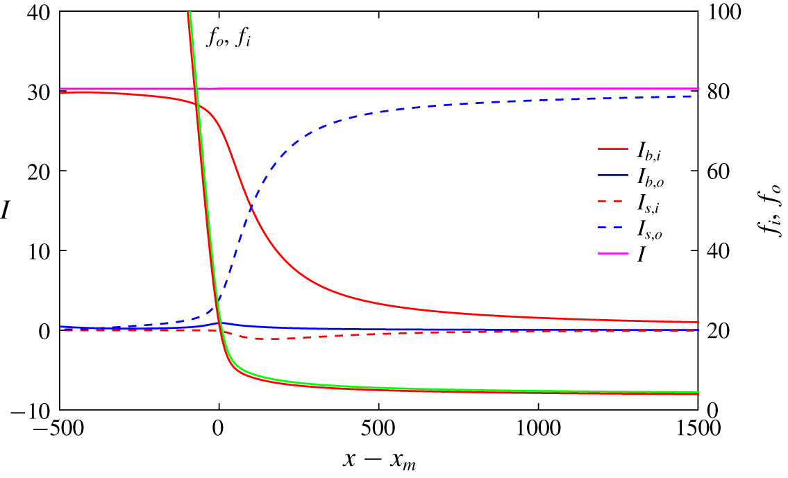
 $Re_{o}=0.64$). The model considers two charge transport mechanisms contributing to the electrical current emitted by the cone–jet: bulk conduction through both liquid subdomains (
 $I_{b,i}$ and
 $I_{b,o}$), and convection of surface charge on both free surfaces (
 $I_{s,i}$ and
 $I_{s,o}$). At any axial position of the cone–jet, each type of current is given by
 $$\begin{eqnarray}I_{s,k}(x)=2\unicode[STIX]{x03C0}f_{k}(x)\unicode[STIX]{x1D70E}_{k}(x)v_{s,k}(x),\quad I_{b,k}(x)=\int _{f_{0k}}^{f_{k}}\unicode[STIX]{x1D705}_{k}^{r}E_{x}(x)2\unicode[STIX]{x03C0}r\,\text{d}r,\end{eqnarray}$$
and, due to conservation of charge, the sum of the four components must be constant and equal to the emitted current,  $I=I_{b,i}(x)+I_{s,i}(x)+I_{b,o}(x)+I_{s,o}(x)$. Here
 $E_{x}$ is the axial component of the electric field, and
 $f_{0k}$ is 0 and
 $f_{i}$ for the inner and outer interfaces, respectively. The axial distributions of the four current components in the transition region are shown in figure 5, together with the position of the free surfaces
 $f_{i}(x)$ and
 $f_{o}(x)$. We use as origin of the axial coordinate the point
 $x_{m}$ where the second derivative of
 $f_{i}(x)$ is maximum. Upstream in the cone the main charge transport mechanism is bulk conduction through the inner liquid, while conduction through the outer liquid is negligible. This is to be expected due to the large area available for conduction through the inner fluid, the much smaller cross-section of the outer subdomain, and the much larger electrical conductivity of the inner liquid. Furthermore, the tangential electric field is constant across the interface
 $f_{i}$, making the axial electric field in the subdomains of both fluids nearly identical in this slender region. As the cross-section of the cone decreases, charge is injected preferentially in the outer free surface, increasing the surface current
 $I_{s,o}$ and decreasing
 $I_{b,i}$ proportionally. Interestingly the surface current in the inner interface is not only small, but also negative. This requires the surface charge in the inner interface to be much smaller than in the outer interface and negative, as the radii and velocities of both free surfaces are nearly identical. The cross-over point of the conduction and surface currents, i.e. the axial position where the conduction and surface currents are equal, is
 $x-x_{m}\simeq 100$.
Axial distribution of the electrical currents in the transition region. Continuous lines represent the ohmic bulk current through the inner and outer liquid,  $I_{b,i}$ and
 $I_{b,o}$. The dashed lines correspond to the electric surface current convected at the interfaces
 $f_{i}$ and
 $f_{o}$,
 $I_{s,i}$ and
 $I_{s,o}$. The total circulating current is
 $I=30.3$. The shape of the interfaces is also plotted. The operating conditions are the same as in figure 4.

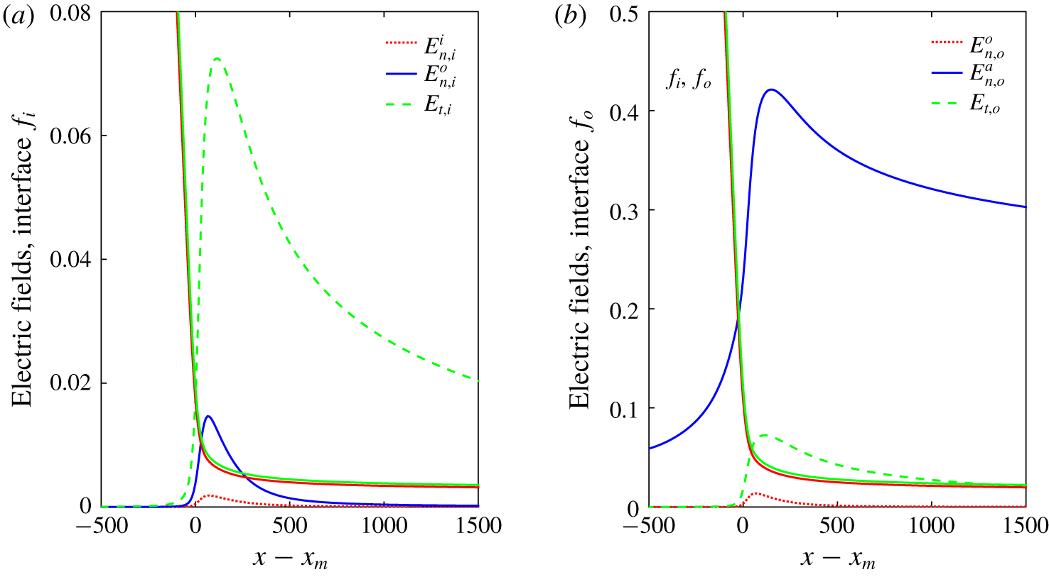
Figure 6 shows the normal components of the electric field across the two free surfaces together with the tangential component. The normal component in the atmosphere side,  $E_{n,o}^{a}$, is significantly larger than the tangential component,
 $E_{t,o}$, and both peak near the current cross-over point (the maximum of
 $E_{n,o}^{a}$ is at
 $x-x_{m}=147$, and that of
 $E_{t,o}$ at 110). This coincides with the profiles of both components in cone–jets of single fluids (Gañán-Calvo Reference Gañán-Calvo1999; Gamero-Castaño & Magnani Reference Gamero-Castaño and Magnani2019). The normal component on the outer surface on the fluid side,
 $E_{n,o}^{o}$, is much smaller than
 $E_{n,o}^{a}$, as should be expected by the large ratio between the fluid residence time,
 $t_{r}$, and the electrical relaxation time,
 $t_{e,o}$, in the outer fluid,
 $t_{e,o}/t_{r}=3.56\times 10^{-4}$. We calculate
 $t_{r}$ as in Ponce-Torres et al. (Reference Ponce-Torres, Rebollo-Muñoz, Herrada, Gañán-Calvo and Montanero2018) by computing the residence time of the outer free surface crossing the cone–jet transition region,
 $$\begin{eqnarray}t_{r}=\int _{s_{i}}^{s_{f}}\frac{\text{d}s}{(\boldsymbol{v}_{o}\boldsymbol{\cdot }\boldsymbol{t}_{o})},\end{eqnarray}$$
where variable  $s$ is the intrinsic coordinate. The interval of the cone–jet transition,
 $[s_{i},s_{f}]$, corresponds to the region in which
 $-0.5\leqslant \log _{10}[(I_{s,o}+I_{s,i})/(I_{b,o}+I_{b,i})]\leqslant 0.5$.
Axial distribution of electric fields at the interfaces (a)  $f_{i}$ and (b)
 $f_{o}$ in the transition region, corresponding to the conditions of figure 4. Dashed green, dotted red and continuous blue lines correspond, respectively, to the tangential, inward normal electric field (subdomain
 $i$ and
 $o$ in (a) and (b), respectively) and outward normal electric field (subdomain
 $o$ in (a) and
 $a$ in (b)). The shape of the interfaces is also plotted.

Therefore, the charge is nearly relaxed everywhere in the free surface and  $\unicode[STIX]{x1D70E}_{o}\cong E_{n,o}^{a}$ (Gamero-Castaño & Magnani Reference Gamero-Castaño and Magnani2019). The normal component on the inner interface on the outer fluid side,
 $E_{n,i}^{o}$, is nearly identical to
 $E_{n,o}^{o}$ due to the small cross-section of the TBP subdomain, and larger than the normal component across the interface
 $E_{n,i}^{i}$. However, and although the ratios of the fluid residence time and the electrical relaxation time are similar for both liquids (
 $t_{e,o}/t_{e,i}=\unicode[STIX]{x1D6FD}_{o}/(\unicode[STIX]{x1D6FD}_{i}\unicode[STIX]{x1D705}_{r})=0.8$), the ratio between the peak values of the normal components is significantly smaller than in the outer free surface:
 $\max (E_{n,i}^{o})/\max (E_{n,i}^{i})=7.9$ and
 $\max (E_{n,o}^{a})/\max (E_{n,o}^{o})=32.1$. In fact, the ratio
 $\max (E_{n,i}^{o})/\max (E_{n,i}^{i})$ needs to be similar to the inverse of the ratio between the electrical conductivities of both fluids,
 $\unicode[STIX]{x1D705}_{i}/\unicode[STIX]{x1D705}_{o}=1/\unicode[STIX]{x1D705}_{r}=7.3$, since the current injected on the outer surface is originated from the bulk current in the inner fluid. This constraint on the ratio
 $E_{n,i}^{o}/E_{n,i}^{i}$ is probably the proximate cause for the negative value of the surface charge. Since the tangential component of the electric field remains continuous across the interfaces and the outer layer is thin,
 $E_{t,i}\simeq E_{t,o}$ are the larger components of the electric field inside the fluid domains along the transition region, consistently with what is found in single-liquid electrosprays.
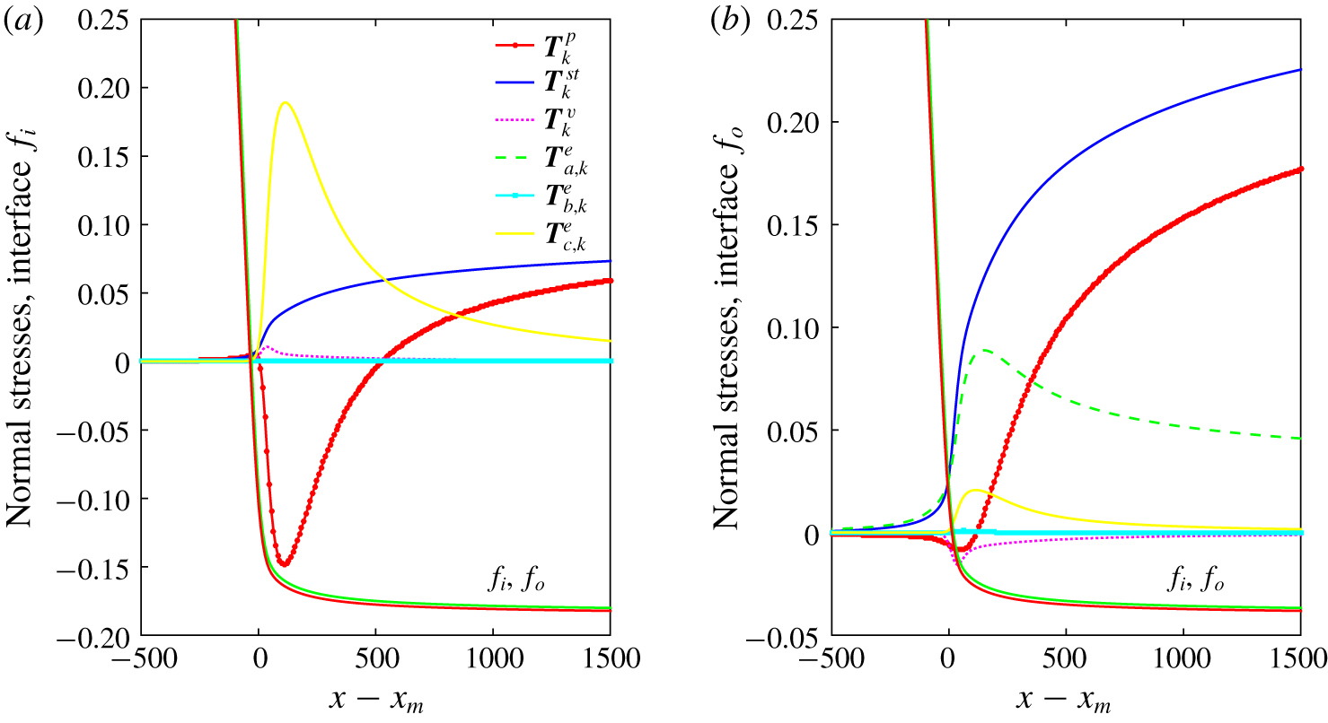
Axial distribution of the different terms of the interfacial normal stress balance (2.5) corresponding to the conditions of figure 4. In panel (a) are shown the terms corresponding to the outer interface,  $f_{o}$, while in panel (b) are shown those of the inner interface,
 $f_{i}$. Labels
 $\{\boldsymbol{T}_{k}^{p};\boldsymbol{T}_{k}^{st};\boldsymbol{T}_{k}^{v};\boldsymbol{T}_{k}^{e}\}$ refer to
 $\{\Vert p\Vert _{k};\unicode[STIX]{x1D6FE}_{k}^{r}\unicode[STIX]{x1D735}\boldsymbol{\cdot }\boldsymbol{n}_{k};\boldsymbol{n}_{k}\boldsymbol{\cdot }\Vert \unicode[STIX]{x1D70F}_{v}\Vert _{k}\boldsymbol{\cdot }\boldsymbol{n}_{k};\boldsymbol{n}_{k}\boldsymbol{\cdot }\Vert \unicode[STIX]{x1D70F}_{v}\Vert _{k}\boldsymbol{\cdot }\boldsymbol{n}_{k}\}$ at interface
 $k$, respectively. Also, in the electric stress term
 $\boldsymbol{T}_{k}^{e}$, we distinguish the normal contributions of the outer and inner sides (subscripts
 $a$ and
 $b$) and the tangential contribution (subscript
 $c$), namely
 $\{\boldsymbol{T}_{a,i}^{e};\boldsymbol{T}_{b,i}^{e};\boldsymbol{T}_{c,i}^{e}\}=\{\unicode[STIX]{x1D6FD}_{o}(E_{n,i}^{o})^{2}/2;\unicode[STIX]{x1D6FD}_{i}(E_{n,i}^{i})^{2}/2;(\unicode[STIX]{x1D6FD}_{i}-\unicode[STIX]{x1D6FD}_{o})E_{t,i}^{2}/2\}$ and
 $\{\boldsymbol{T}_{a,o}^{e};\boldsymbol{T}_{b,o}^{e};\boldsymbol{T}_{c,o}^{e}\}=\{(E_{n,o}^{a})^{2}/2;\unicode[STIX]{x1D6FD}_{o}(E_{n,o}^{o})^{2}/2;(\unicode[STIX]{x1D6FD}_{o}-1)E_{t,o}^{2}/2\}$ on the inner and outer interfaces, respectively. The shape of the interfaces is also plotted.

In figure 7 we plot the axial variation of the normal stresses acting on both free surfaces, i.e. the terms of (2.5). In the figure we have labelled as  $\boldsymbol{T}^{p}$,
 $\boldsymbol{T}^{st}$,
 $\boldsymbol{T}^{v}$ and
 $\boldsymbol{T}^{e}$, the pressure, surface tension, viscous and electric stress terms, respectively. Also, in the electric stress term
 $\boldsymbol{T}^{e}$, we distinguish the normal contributions of the outer and inner sides (subscripts
 $a$ and
 $b$) and the tangential contribution (subscript
 $c$), namely
 $\{\boldsymbol{T}_{a,i}^{e};\boldsymbol{T}_{b,i}^{e};\boldsymbol{T}_{c,i}^{e}\}=\{\unicode[STIX]{x1D6FD}_{o}(E_{n,i}^{o})^{2}/2;\unicode[STIX]{x1D6FD}_{i}(E_{n,i}^{i})^{2}/2;(\unicode[STIX]{x1D6FD}_{i}-\unicode[STIX]{x1D6FD}_{o})E_{t,i}^{2}/2\}$ and
 $\{\boldsymbol{T}_{a,o}^{e};\boldsymbol{T}_{b,o}^{e};\boldsymbol{T}_{c,o}^{e}\}=\{(E_{n,o}^{a})^{2}/2;\unicode[STIX]{x1D6FD}_{o}(E_{n,o}^{o})^{2}/2;(\unicode[STIX]{x1D6FD}_{o}-1)E_{t,o}^{2}/2\}$ on the inner and outer interfaces, respectively. The stresses associated with the normal component of the electric field in the inner side of the interface,
 $\boldsymbol{T}_{b}^{e}$, are negligible everywhere, while the viscous stress only displays a relatively small peak near
 $x_{m}$.
In the outer surface  $f_{o}$ the most important terms in the balance are the pressure,
 $\boldsymbol{T}_{o}^{p}$, the electrostatic suction caused by the outward normal electric field,
 $\boldsymbol{T}_{a,o}^{e}$, and the surface tension,
 $\boldsymbol{T}_{o}^{st}$. Up to
 $x-x_{m}\simeq 40$ the surface tension almost fully balances this electrostatic suction,
 $\boldsymbol{T}_{o}^{st}\simeq \boldsymbol{T}_{a,o}^{e}$, making the pressure jump across the interface negligible; this is consequence of the near-equipotentiality of the surface up to this point. Further downstream,
 $E_{t,o}$ increases, the electrostatic suction
 $\boldsymbol{T}_{c,o}^{e}$ becomes significant, and its combination with the
 $\boldsymbol{T}_{a,o}^{e}$ term forces the pressure to become slightly negative to fulfil the balance of normal stresses. Once
 $E_{t,o}$ and its associated stress become negligible further downstream in the jet, the surface tension is balanced by the pressure and a smaller value of the electrostatic suction,
 $\boldsymbol{T}_{a,o}^{e}$.
The balance in the inner interface  $f_{i}$ is quite different: due to the smallness of either normal electric field compared to
 $E_{t,i}$,
 $\boldsymbol{T}_{c,i}^{e}$ is the only important electrostatic stress. Furthermore, because water has a large relative permittivity, this term becomes a dominant suction, which needs to be balanced by a large negative pressure drop across the interface. The surface tension
 $\boldsymbol{T}_{i}^{st}$ is a significant but smaller term: the curvatures of both surfaces are nearly equal,
 $\unicode[STIX]{x1D735}\boldsymbol{\cdot }\boldsymbol{n}_{i}\simeq \unicode[STIX]{x1D735}\boldsymbol{\cdot }\boldsymbol{n}_{o}$, but the interface tension in the TBP–water interface is a few times smaller than the surface tension of TBP.
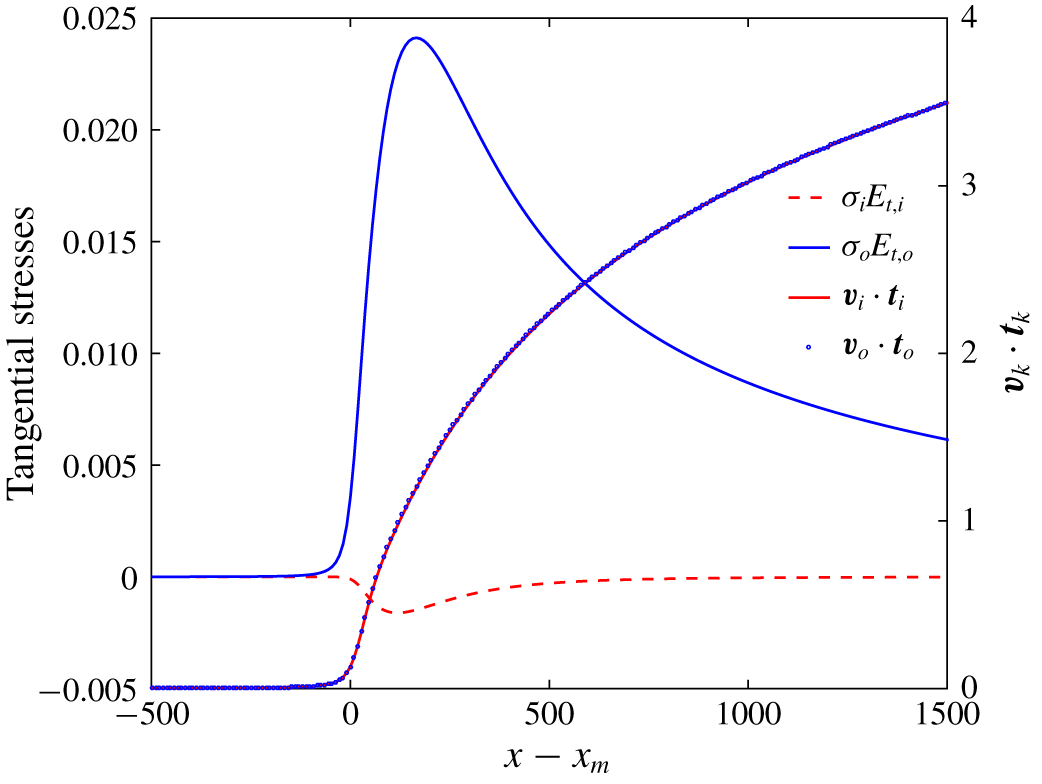
Figure 8 shows the electric tangential stresses and the surface velocity in both interfaces. The tangential stresses in the outer surface are small compared to the normal ones, while, due to the small values of  $\unicode[STIX]{x1D70E}_{i}$, the tangential stress in the inner interface is negligible. On the other hand, the velocity in any cross-section of the jet is for all purposes uniform, regardless of the fluid domain, i.e. viscous diffusion efficiently transfers momentum across the jet section. The velocity increases continuously along the jet due to the electrostatic acceleration by the axial electric field.
Axial distribution of the electrical tangential stress (left axis) and tangential velocity (right axis) in interfaces  $f_{o}$ and
 $f_{i}$, corresponding to the conditions of figure 4.

5.2 Dependence on the relative conductivity $\unicode[STIX]{x1D705}_{r}$

Figures 9–11 analyse the solution at varying  $\unicode[STIX]{x1D705}_{r}$, for fixed values of
 $Q_{i}=171$,
 $Q_{o}=44$ and
 $\unicode[STIX]{x1D719}=197$ (density and surface tension ratio, as mentioned, are also kept constant at
 $\unicode[STIX]{x1D70C}_{r}=0.976$ and
 $\unicode[STIX]{x1D6FE}_{r}=0.29$) and the same geometry as in figures 4–8. Figure 9 shows the effect of varying
 $\unicode[STIX]{x1D705}_{r}$ on the position of the interfaces in the transition region:
 $\unicode[STIX]{x1D705}_{r}$ is varied by three orders of magnitude above and below the reference value
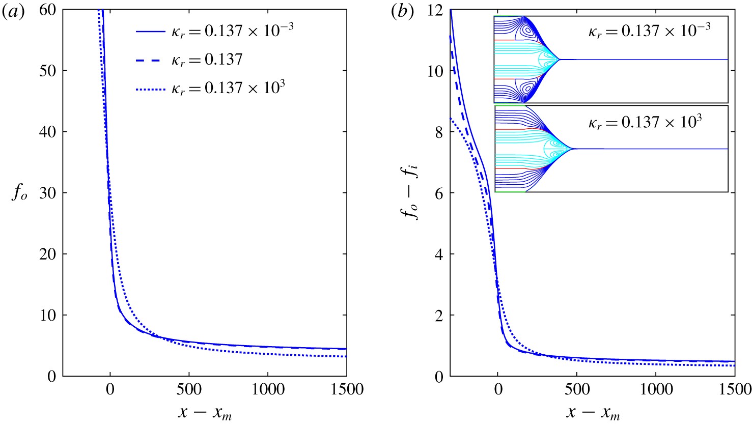
 $\unicode[STIX]{x1D705}_{r}=0.137$ used in § 5.1. Figure 9(b) also contains two insets with the streamlines (those for
 $\unicode[STIX]{x1D705}_{r}=0.137$ are given in figure 4). The positions of the two surfaces and the streamline patterns including recirculation areas remain unchanged when lowering
 $\unicode[STIX]{x1D705}_{r}$ below 0.137, while there is a significant difference for
 $\unicode[STIX]{x1D705}_{r}=0.137\times 10^{3}$: in this case the recirculation region in the outer fluid disappears, and both free surfaces transition from cone to jet following smoother trajectories (the second derivative of the interfaces, e.g.
 $f_{o}^{\prime \prime }(x)$, are lower around
 $x_{m}$, and the diameter of the jet becomes smaller downstream).
Influence of  $\unicode[STIX]{x1D705}_{r}$ in the geometry of the transition region. In panels (a) and (b) are shown the position of the interface and the width of the layer, respectively. The inset of panel (b) shows streamlines and interface for
 $\unicode[STIX]{x1D705}_{r}=0.137\times 10^{-3}$ and
 $0.137\times 10^{3}$.

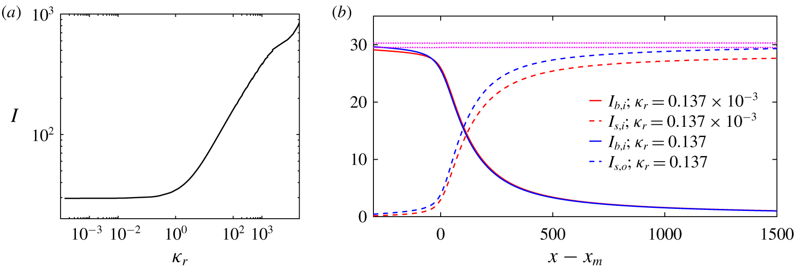
Figure 10(a) plots the total current as a function of  $\unicode[STIX]{x1D705}_{r}$, which shows a similar behaviour, i.e. for
 $\unicode[STIX]{x1D705}_{r}\lesssim 0.2$ the current remains unchanged, while for larger values of
 $\unicode[STIX]{x1D705}_{r}$ the current increases with the conductivity of the outer fluid. Figure 10(b) explains this trend for the total current, by plotting the profiles of the dominant bulk and surface currents for several values of
 $\unicode[STIX]{x1D705}_{r}$. For
 $\unicode[STIX]{x1D705}_{r}=0.137\times 10^{-3}$ the conductivity of the outer fluid is much smaller than that of the inner one and, since the tangential component of the electric field is similar through the cross-section of the transition region, conduction takes place mostly through the inner fluid and
 $I_{b,i}$ is the dominant bulk conduction current. On the other hand, the conductivity of the outer fluid is so low that injection of charge onto the outer surface from the inner fluid is small, and most of the surface current is locked in the inner interface (
 $I_{s,i}$ is the dominant surface current term). In this case the outer liquid behaves like a dielectric shell devoid of free charge surrounding the inner fluid, which is where the electric stresses are directly applied. In particular, the inner fluid is accelerated by the tangential electric stress acting on the inner interface, which in turn drags the outer fluid by nearly complete viscous diffusion of momentum.
(a) Total current  $I$ versus
 $\unicode[STIX]{x1D705}_{r}$ in log scale for
 $Q_{o}=44$ and
 $Q_{i}=171$. (b) Axial distribution of relevant electrical currents in the transition region for the conductivities
 $\unicode[STIX]{x1D705}_{r}=0.137\times 10^{-3}$ (red lines) and
 $\unicode[STIX]{x1D705}_{r}=0.137$ (blue lines) being
 $Q_{o}=44$ and
 $Q_{i}=171$. Continuous, dashed and dotted lines correspond to bulk, interfacial and total electric current, respectively. The
 $I_{b,i}$ curve is shown for both conductivities, while
 $I_{s,i}$ and
 $I_{s,o}$ are shown for
 $\unicode[STIX]{x1D705}_{r}=0.137\times 10^{-3}$ and
 $\unicode[STIX]{x1D705}_{r}=0.137$, respectively.

For  $\unicode[STIX]{x1D705}_{r}=0.137$ the conductivity of the outer fluid is still significantly smaller, so that
 $I_{b,i}$ remains the dominant component of the bulk conduction current and continues fixing the total current of the electrospray. Yet, the smaller disparity between the electrical conduction does not prevent the injection of charge on the outer surface, and
 $I_{s,o}$ becomes the larger of the two surface currents. In this case the tangential electric stress acts on the outer surface, and both fluids are accelerated by viscous diffusion from that surface.
Finally, for  $\unicode[STIX]{x1D705}_{r}=0.137\times 10^{3}$ the conductivity of the outer fluid is much larger. In this case the coaxial electrospray operates very much like the cone–jet of a single liquid with the electrical properties of the outer fluid, and a flow rate that is the sum of those for the two fluids.
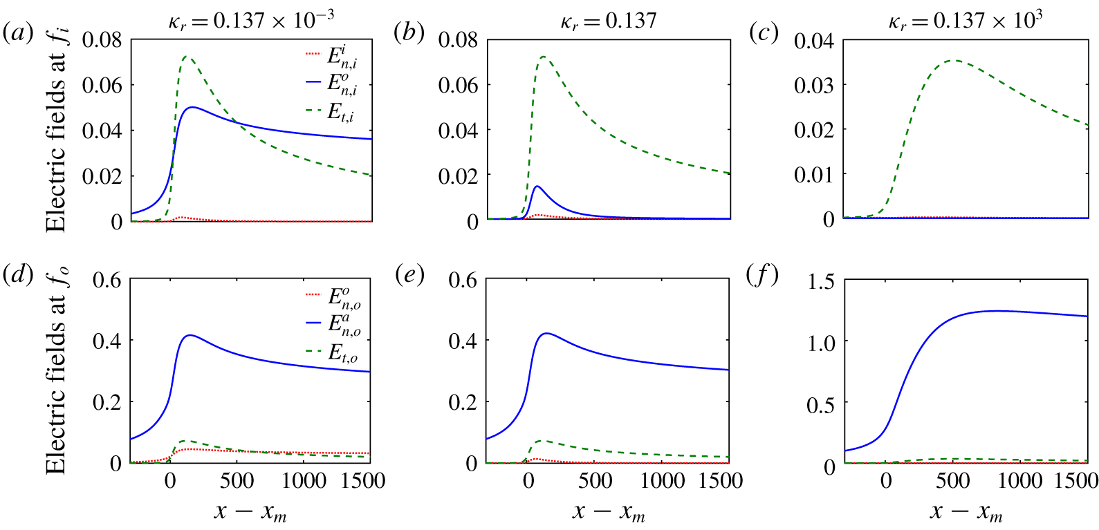
Axial distribution of the electric components at the interfaces. Inward and outward normal electric fields correspond to the red dotted and blue continuous lines, respectively; tangential electric field corresponds to the dashed green line. Panels (a–c) correspond to interface  $f_{i}$, while panels (d–f) correspond to
 $f_{o}$. Panels (a,d), (b,e) and (c,f) correspond to relative conductivities
 $\unicode[STIX]{x1D705}_{r}=0.137\times 10^{-3}$, 0.137 and
 $0.137\times 10^{3}$, respectively.

Another interesting feature is the ability of the surface charge on  $f_{o}$ to screen the normal component of the electric field in the gas phase, so that it does not penetrate into the fluid. The degree of screening, or equivalently the degree to which the surface charge is relaxed, depends on the ratio between the fluid residence time and the electrical relaxation time, equation (5.2). The values of this ratio for the three relative conductivity cases discussed in this section are
 $\{\unicode[STIX]{x1D705}_{r},t_{e,o}/t_{r}\}=\{0.137\times 10^{-3},0.35\}$,
 $\{0.137,3.6\times 10^{-4}\}$ and
 $\{0.137\times 10^{3},4.7\times 10^{-8}\}$. Clearly the surface charge is for all purposes in equilibrium when
 $\unicode[STIX]{x1D705}_{r}=0.137\times 10^{3}$, and consequently the component of the electric field normal to
 $f_{o}$ everywhere in the transition region should be negligible, as can be observed in figure 11(d). On the other hand, for
 $\unicode[STIX]{x1D705}_{r}=0.137\times 10^{-3}$ the surface charge on
 $f_{o}$ is far from equilibrium, and
 $E_{n,o}^{o}\cong \unicode[STIX]{x1D6FD}_{o}^{-1}E_{n,o}^{a}$. The axial component of the electric field across any section in the transition region, nearly aligned with the tangential electric field
 $E_{t,i}$, is nearly uniform. Figure 11 shows the dominant components of the electric field for the three values of the relative conduction
 $\unicode[STIX]{x1D705}_{r}$. Finally, the increasing degree of relaxation of the outer surface charge
 $\unicode[STIX]{x1D70E}_{o}$ at increasing
 $\unicode[STIX]{x1D705}_{r}$ is responsible for the smoother transition of the surface from cone to jet observed in figure 9: the increased relaxation requires an earlier departure of the position of the surface from the conical shape consistent with an equipotential solution.
5.3 The role of outer and inner flow rates, $Q_{o}$ and $Q_{i}$


In this section we study the effect of varying the flow rates of both fluids at fixed relative conductivity and emitter potential, using as reference state the conditions simulated in § 5.1:  $\unicode[STIX]{x1D705}_{r}=0.137$,
 $Q_{i}=171$,
 $Q_{o}=44$ and
 $\unicode[STIX]{x1D719}=197$. Section 5.2 discusses how these parameters lead to a coaxial electrospray that operates similarly to a cone–jet of the inner liquid, with an outer liquid that forms a shell around the inner liquid and has a small effect on the dynamics. However, and unlike in the case of
 $\unicode[STIX]{x1D705}_{r}=0.137\times 10^{-3}$, the role played by this outer shell is not completely negligible, as
 $\unicode[STIX]{x1D705}_{r}$ is sufficiently high to make
 $I_{s,o}$ the dominant surface current. The inset of figure 3 shows the current as a function of
 $\widetilde{Q}_{i}^{1/2}$, to test the hypothesis that under these conditions the coaxial electrospray is behaving similarly to a cone–jet of the inner fluid (the flow rate of the outer liquid is constant and equal to
 $Q_{o}=44$ (
 $60~\unicode[STIX]{x03BC}\text{l}~\text{h}^{-1}$) and
 $Q_{o}=147$ (
 $200~\unicode[STIX]{x03BC}\text{l}~\text{h}^{-1}$)). The data follow the dimensionless
 $I=\unicode[STIX]{x1D6FC}Q_{i}^{1/2}$ law that characterizes traditional cone–jets, with a constant of proportionality that depends slightly on the outer flow rate,
 $\unicode[STIX]{x1D6FC}=2.79$ and 2.96 for
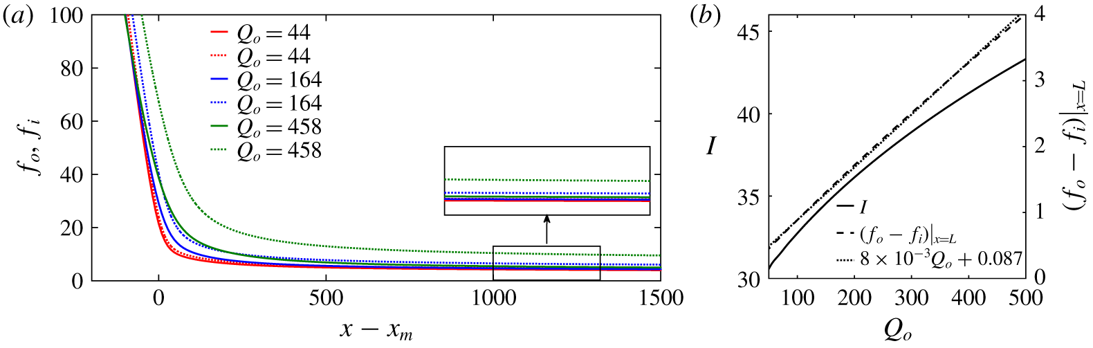
 $Q_{o}=147$ and 144, respectively. These figures are near the average value of 2.6 obtained from experimental measurements of single-phase electrosprays of a large number of liquids. Figure 12(b) shows the dependence of
 $I$ on
 $Q_{o}$ at fixed flow rate of the inner liquid,
 $Q_{i}=171$. The dependence is, as expected, significantly weaker than the dependence on
 $Q_{i}$; an increment of the flow rate
 $Q_{o}$ by a decade turns out to increase the current by just 50 %.
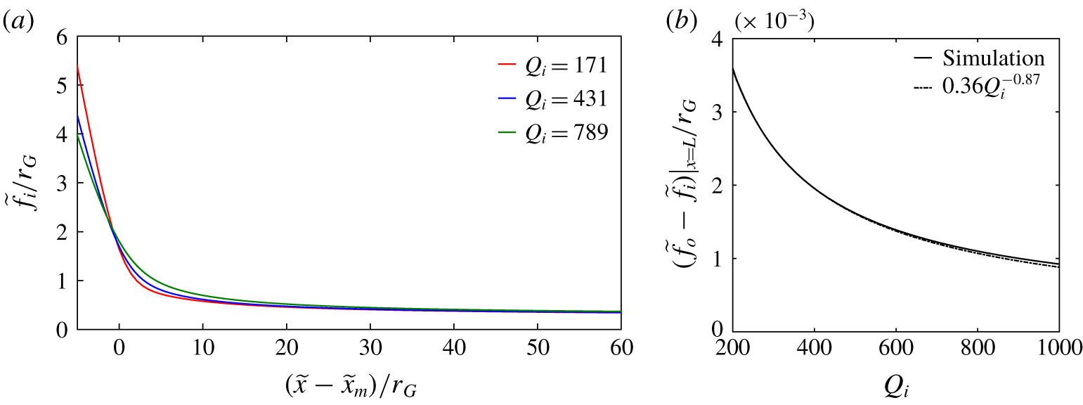
Figure 13(a) shows the position of the two interfaces normalized with the characteristic length typical of traditional cone–jets,  $r_{G}$, used already in (5.2), for several values of
 $Q_{i}$ and fixed
 $Q_{o}=44$. Despite the large variation of
 $Q_{i}$, this scaling collapses the three
 $f_{i}(x)$ profiles, confirming again that this coaxial cone–jet is operating like a traditional cone–jet of the inner fluid. Since the flow of the outer liquid is kept constant and the axial velocity is uniform and the same for both fluids, the thickness of the outer shell made dimensionless with
 $r_{G}$ should decrease with
 $Q_{i}$ as
 $(f_{o}-f_{i})/r_{G}\asymp Q_{i}^{-1}$, very close to the fitting observed in the simulations (see figure 13b).
(a) Interface positions for three different outer flow rates  $Q_{o}=44$ (red), 164 (blue) and 458 (green). The inset shows a magnification of the jet region. Continuous and dashed lines correspond to inner and outer interfaces. (b) The left
 $y$-axis shows the total current
 $I$ versus
 $Q_{o}$, while on the right
 $y$-axis is plotted the width of the layer evaluated at the end of the computational domain,
 $(f_{o}-f_{i})|_{x=L}$. In both plots, the inner flow rate is
 $Q_{i}=171$.

(a) Inner interface position,  $\widetilde{f}_{i}/r_{G}$, for three different values of
 $Q_{i}=171$, 431 and 789. The length scale
 $r_{G}$ is given in (5.2). (b) Dimensionless width of the layer evaluated at the end of the computational domain,
 $(\widetilde{f}_{o}-\widetilde{f}_{i})_{x=L}/r_{G}$, as a function of the inner flow rate
 $Q_{i}$. Simulations fit the regression
 $(\widetilde{f}_{o}-\widetilde{f}_{i})_{x=L}/r_{G}\simeq 0.46Q_{i}^{-0.87}$.

6 Conclusions and outlook
While prior studies have explored miscible liquid systems (Xu et al. Reference Xu, Qin, Yin, Hua, Pack and Wang2013) or have drastically reduced the problem to a 1-D simulation (Higuera Reference Higuera2007) where the core fluid is a perfect dielectric, in this work a complete model of coaxial electrosprays applicable to general 2-D (axisymmetric) geometries in the limit of zero net bulk charges (charge relaxation hypothesis), constant electrical permittivities and conductivities, and strict immiscibility of the liquids is presented. A robust numerical simulation method is applied in this work, which was first proposed by Herrada et al. (Reference Herrada, Lopez-Herrera, Gañan-Calvo, Vega, Montanero and Popinet2012), improved by Herrada & Montanero (Reference Herrada and Montanero2016), and subsequently applied to other problems with the presence of capillary surfaces (Ponce-Torres et al. Reference Ponce-Torres, Vega and Montanero2016, Reference Ponce-Torres, Montanero, Herrada and Vega2017; Cruz-Mazo et al. Reference Cruz-Mazo, Herrada, Gañán-Calvo and Montanero2017). The method proposed maps the three physical subdomains into three rectangles corresponding to both inner and outer electrosprayed liquids and the passive environment, with a consistent transformation of coordinates. The discretization of the equations and subsequent solution are performed following the procedures described in previous works (Herrada & Montanero Reference Herrada and Montanero2016).
In this work an illustrative range of a few fundamental variables, namely the electrical permittivities and conductivities of the liquids and their relative weight and their relevant effects, has been analysed. The effect of other variables within the ample spectrum that coaxial electrospray implies (densities, viscosities, surface tensions, geometries of the capillaries, etc.) is a matter of subsequent more specific studies, once the validity of a tool of analysis like the one proposed here is verified.
A number of experimental realizations are successfully compared to the numerical simulations. Special attention is paid to describe the whole physics rendered by the model, for a specific choice of experimental parameters. Subsequently, the influence of both the ratio of conductivities and flow rates on the different physical variables (e.g. electric fields and currents) is analysed, recovering either the asymptotic limit of the outer driving liquid experimentally described in the literature López-Herrera et al. (Reference López-Herrera, Barrero, López, Loscertales and Márquez2003), or when the coaxial electrospray behaves as the well-known single-phase electrospray of the inner liquid.
One of the interesting findings of our study is the surprising result of the existence of a region of the inner surface where the charge can be negative, which could not be expected unless the complete problem was resolved. This implies a physicochemical degree of freedom that is absent in single-liquid electrosprays. It means that somewhere in the inner liquid domain, the charge balance that imposes strict conditions on the moving liquid phases may lead to those observed negative charges at the interface of the immiscible liquids. That balance is determined by the conductivities and permittivities of both liquids and their relative values in the absence of surface conduction effects (Burcham & Saville Reference Burcham and Saville2002), which brings about some deeper considerations on the assumptions made in the model, and possible extensions, as follows.
(i) The net bulk charge is assumed to be zero in both domains. Here, the numerical model does not impose limitations on the source of counter-ions to feed this inner negative surface charge, but assumes that any charge imbalance appearing in the bulk should be small as implied by charge relaxation. The charge relaxation and its implications have been extensively discussed in the existing literature, assuming constant electrical permittivities and conductivities. It is noteworthy to mention here that electrolyte solutions in polar liquids are used in most electrospray formulations. The dissociation times of polar liquids are much smaller than those of charge relaxation. One may argue that any local (small) bulk charge imbalance below a certain threshold depending on the potential of dissociation would be partly but nearly instantaneously restored by dissociation.
(ii) The electrical conductivity, as strictly defined in Saville (Reference Saville1997) (see also Gañán-Calvo et al. (Reference Gañán-Calvo, López-Herrera, Herrada, Ramos and Montanero2018)), involves the mobilities and concentrations of both ionic species present in each domain. As long as those mobilities are similar for the ionic species present in the liquid, and their concentrations remain nearly constant everywhere, the assumption of a constant value of the liquid conductivities is implicit with the assumption of zero net bulk charge. Again, since electrical conductivity is a function of temperature and concentration for electrolytes in solution, its value should be constant everywhere in the liquid domain except in the vicinity of the interfaces at distances comparable to the Debye length (Saville Reference Saville1997). Thus, as long as surface conduction associated with tangential electric fields acting on the surface charge layer can be neglected compared to the bulk conduction, which implies certain restrictions on the thermal diffusivity
$D_{k}$ of the ions in the liquids as $D_{k}\ll d_{e}^{2}/t_{e}(E_{n,k}/E_{t,k})^{2}$, our results would render realistic predictions. A fundamental question arises on the possible extension of the methods proposed here and the basic assumptions of the leaky dielectric model beyond conditions where hydrodynamic and charge relaxation times become comparable. In electrospray configurations, the transition region implies an extraordinarily rapid stretching of the liquid. This made some authors think about the possibility that the situation reached upstream with a quasi-neutral bulk and a surface charge layer could be frozen (Fernandez de la Mora & Loscertales Reference Fernandez de la Mora and Loscertales1994; Fernández de la Mora Reference Fernández de la Mora2007) as the liquid approaches that region. This postulate would render thermal diffusion a negligible effect even in unsteady situations (Gañán-Calvo et al. Reference Gañán-Calvo, López-Herrera, Rebollo-Muñoz and Montanero2016), which in turn would make global linear stability analysis like the one presented in Ponce-Torres et al. (Reference Ponce-Torres, Rebollo-Muñoz, Herrada, Gañán-Calvo and Montanero2018) amply valid for the coaxial electrospray system studied here. However, this is still an unresolved matter of fundamental interest. Indeed, we have taken special care to select our parametric ranges of study in this work within regions where stability is experimentally assured.(iii) The condition of immiscibility between the two liquids creates a barrier for the ionic species at the free interface. That physicochemical barrier is assumed to be higher than any other potential for the ionic species in each liquid domain, implying that ionic cross-contamination is absent between the two domains, independently of the concentration of charges (either positive or negative) at the interface. However, the surface charge conservation equation used in this work does not preclude ion migration and cross-contamination, as long as that is restricted to the charge layers at the liquid–liquid interface (again, in the absence of surface conduction effects). The addition of non-negligible surface conductivity is a matter of subsequent analysis. In particular, another fundamental question here is whether surface conductivity could be assumed as a constant property along the cone–jet transition in electrospray configurations.
(iv) The values of the liquid permittivities, which reflect the degree of molecular polarity, are assumed to be not only constant but also unable to alter the different molecular potential conditions necessary to fulfil the other discussed assumptions of the model.


In summary, we claim that our findings, counterintuitive as they may appear, should reflect the physical reality as long as the liquid formulations comply with the relatively general conditions entailed by the assumption of zero net bulk charge and strict immiscibility. Notwithstanding that, a rich variety of physicochemical and surface electrochemistry processes opens up for further exploration. In particular, the global stability analysis of the system studied here could be one of the immediate tasks of future studies.
Acknowledgements
This work was supported by the Ministerio de Economía y Competitividad, Plan Estatal 2013-2016 Retos, project DPI2016-78887-C3-1-R. J.M.L.-H. wishes to acknowledge the financial support of the Ministerio de Educación, Cultura y Deporte of the Kingdom of Spain through the programme ‘Salvador de Madariaga’.