
1. Introduction
Nanoscale confined flows (NCFs) are prevalent in nature and technologies, including solar steam generation (Ghasemi et al. Reference Ghasemi, Ni, Marconnet, Loomis, Yerci, Miljkovic and Chen2014), high-performance nanocooling (Lu et al. Reference Lu, Kinefuchi, Wilke, Vaartstra and Wang2019; van Erp et al. Reference van Erp, Soleimanzadeh, Nela, Kampitsis and Matioli2020), nanoprinting (Fernández-Toledano et al. Reference Fernández-Toledano, Braeckeveldt Bertrand and De Coninck2020) and hydrogen/carbon dioxide storage (Navaid, Emadi & Watson Reference Navaid, Emadi and Watson2023). These flows exhibit multiscale characteristics (Bhadauria & Aluru Reference Bhadauria and Aluru2017; Shan et al. Reference Shan, Wang, Zhang and Guo2020), making the standard Navier–Stokes–Fourier (NSF) equations (Torrilhon Reference Torrilhon2016; Hattori Reference Hattori2023) inadequate and molecular dynamics (MD) simulations computationally prohibitive (Sadr, Pfeiffer & Gorji Reference Sadr, Pfeiffer and Gorji2021). This highlights the need for a molecular kinetic model that fills the gap between the molecular-scale dynamics and continuum hydrodynamics.
The NCFs exhibit distinct features due to surface confinement, posing significant challenges for molecular kinetic modelling. First, the interactions between surface and fluid molecules create notable inhomogeneities in fluid density and transport coefficients (Guo, Zhao & Shi Reference Guo, Zhao and Shi2005; Bhadauria, Sanghi & Aluru Reference Bhadauria, Sanghi and Aluru2015) within the attraction range
 $h\lt H_{att}$
, as shown in figure 1(a) where
 $h$
denotes the distance from the surface. Second, these inhomogeneities influence fluid–solid collision dynamics including velocity slip and temperature jump at
 $h=H_{ex}$
(Hadjiconstantinou Reference Hadjiconstantinou2024), where
 $H_{ex}$
is an equivalent fluid–solid volume exclusion region as to be determined in § 2.2.1. Additionally, non-hydrodynamic effects at the fluid–solid interface depend on the solid’s composition (Martini et al. Reference Martini, Hsu, Patankar and Lichter2008a
). Finally, real fluid effects, largely ignored in gas kinetic theory, influence the static structure and dynamics of nanoscale flows and further enhance the complexity of NCFs (Shan et al. Reference Shan, Su, Gibelli and Zhang2023b
; Han et al. Reference Han, Xia, Chen, Wu, Li, Wei, Zheng and Ma2025). It is essential to address these issues and develop accurate molecular kinetic models to account for fluid–fluid (real fluid effects) and fluid–surface interactions.
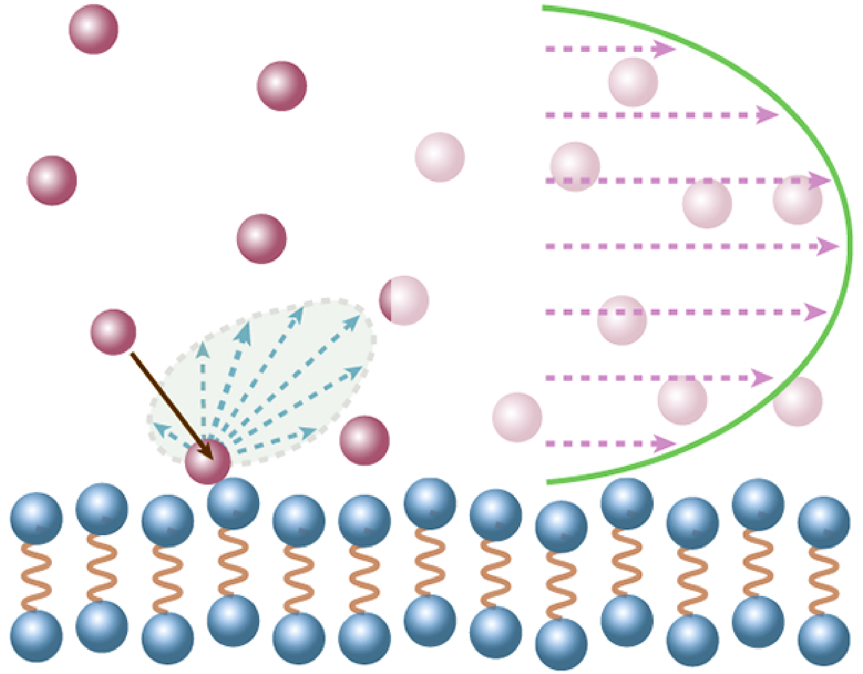
(a) The range of fluid–surface scattering at
 $h=H_{ex}$
, fluid–surface attraction (
 $h\lt H_{att}$
) and bulk fluid (
 $h\gt H_{att}$
) regions in NCFs; (b) determination of the hydrodynamic wall location, with
 $H_1$
and
 $H_2$
representing two extreme cases where fluid molecules collide with the solid surface; (c) schematic of a fluid molecule colliding through the hydrodynamic wall, with solid molecules remaining at Maxwellian equilibrium; (d) specular reflection on a perfectly smooth surface; (e) diffuse reflection on a perfectly rough surface; (f) MD simulation set-up.

Existing kinetic models for fluid–surface interactions often neglect their strong coupling with fluid transport, an approach that is acceptable for macroscopic flows where the region within the influence of surface potential (
 $H_{att}$
) is small relative to the confinement space (
 $H$
). In such cases, a conventional boundary condition suffices to describe interfacial physics (Cercignani Reference Cercignani1988). However, for NCFs where
 $H_{att}$
is comparable to
 $H$
, this simplification becomes problematic. Furthermore, traditional kinetic theory (Cercignani Reference Cercignani1988) for dilute-gas–surface interactions fails to capture fluid inhomogeneities (Hadjiconstantinou Reference Hadjiconstantinou2024) and composition-dependent non-hydrodynamic effects (Martini et al. Reference Martini, Roxin, Snurr, Wang and Lichter2008a
). Conversely, slip models based on molecular theory/mechanics for dense-liquid–surface interactions depend heavily on empirical parameters and are constrained to isothermal conditions (Shan et al. Reference Shan, Wang, Wang, Zhang and Guo2022; Hadjiconstantinou Reference Hadjiconstantinou2024). Therefore, there remains a lack of a comprehensive theoretical framework that can accurately describe non-hydrodynamic effects in both dilute and dense fluids, especially in tightly confined systems where both real fluid effects and fluid–surface interactions play critical roles in shaping the behaviour of NCFs.
In this work, we present a molecular kinetic model for NCFs that can accurately describe fluid–surface molecular interactions and capture real fluid effects. An appropriate consideration of fluid–surface interactions in the transport equation, as presented in our model, is vital for accurately predicting velocity slip and temperature jump at the fluid–solid interface. By addressing the research challenges associated with NCFs, this new model enables a mesoscopic simulation tool to advance our understanding of NCFs and develop nanoflow technologies.
The remainder of the paper is organised as follows. In § 2, we present a straightforward yet effective framework for modelling fluid–fluid and fluid–surface interactions in NCFs consistently. In § 3, we introduce a tractable molecular kinetic model that can capture both intrinsic and apparent non-hydrodynamic effects as well as real fluid behaviours, thereby addressing the challenge of defining proper boundary conditions for flows involving strongly inhomogeneous fluids. The intrinsic non-hydrodynamic effects arise from the mismatch between fluid and solid properties at their interface, while the apparent non-hydrodynamic effects are deviations observed by extrapolating from the Navier–Stokes predictions at the bulk. The numerical set-ups and solving procedures for both the molecular kinetic model and MD simulations are detailed in § 4.1. The main features of NCFs and the Knudsen paradox phenomena are investigated in §§ 4.2 and 4.3, respectively, through comparisons between MD simulations and the molecular kinetic model, demonstrating the accuracy and capability of the proposed kinetic model. A comparison with previous kinetic models is conducted at the end of § 4. Finally, the paper concludes in § 5, where the novelty and potential extensions of the proposed molecular kinetic model are discussed.
2. Modelling fluid–fluid and fluid–surface interactions
The behaviour of NCFs is largely determined by fluid–surface interactions, causing density variations (i.e. the layering structure) that lead to changes in transport properties near solid surfaces (Vanderlick, Scriven & Davis Reference Vanderlick, Scriven and Davis1989; Hadjiconstantinou Reference Hadjiconstantinou2024). As the thickness of adsorbed fluids become non-negligible, fluid–surface molecular interactions cannot be solely described by traditional boundary conditions. According to the dense fluid theory (Chapman & Cowling Reference Chapman and Cowling1990), the size of a fluid molecule
 $\sigma _f$
needs explicit consideration when it is comparable to either the mean free path
 $\ell$
or the confinement size
 $H$
. In such cases, the size of solid molecules
 $\sigma _s$
also becomes critical, as
 $\sigma _s$
and
 $\sigma _f$
are often of the same magnitude. Therefore, fluid–surface molecular interactions should be explicitly modelled in the transport equation. Given that a fluid molecule simultaneously interacts with both fluid and solid molecules in NCFs, the fluid transport equation can be expressed as
 \begin{equation} D_t f =Q_{\textit{ff}} + Q_{\textit{fs}}, \end{equation}
where
 $D_t=\partial _t + \boldsymbol{\xi }\cdot \nabla$
is the material derivative,
 $f=f(\boldsymbol{r}, \boldsymbol{\xi }, t)$
is the velocity distribution function (VDF) of a fluid molecule with velocity
 $\boldsymbol{\xi }$
at position
 $\boldsymbol{r}$
and time
 $t$
. The terms
 $Q_{\textit{ff}}$
and
 $Q_{\textit{fs}}$
describe non-local collision effects for fluid–fluid (
 $\textit{ff}$
) and fluid–solid (
 $fs$
) interactions, respectively. Notably, in conventional kinetic theory,
 $Q_{\textit{fs}}$
reduces to a boundary condition.
2.1. Fluid–fluid interactions
According to the kinetic theory for dense fluids and mean-field theories, the fluid–fluid interactions
 $Q_{\textit{ff}}$
can be decomposed into short-range repulsive interactions
 $Q_{\textit{ff}}^{\textit{sg}}$
for
 $|\boldsymbol{r}'|=|\boldsymbol{r}_2-\boldsymbol{r}_1|\lt \sigma _f$
and long-range attractive interactions
 $Q_{\textit{ff}}^{lg}$
for
 $|\boldsymbol{r}'| \geqslant \sigma _f$
. This decomposition (Shan et al. Reference Shan, Su, Gibelli and Zhang2023b
) is expressed as
 \begin{align} Q_{\textit{ff}} & = Q_{\textit{ff}}^{\textit{sg}} + Q_{\textit{ff}}^{lg}, \end{align}
 \begin{align} Q_{\textit{ff}}^{\textit{sg}} & = \chi (\bar {n}) Q_{\textit{ff}}^0 + Q_{\textit{ff}}^1, \end{align}
 \begin{align} Q_{\textit{ff}}^{lg} & = m^{-1}\nabla _{\boldsymbol{\xi }}f\cdot \nabla \phi _{\textit{ff}}^{lg}, \end{align}
where
 $m$
is the mass of a fluid molecule,
 $\chi$
is the radial distribution function (Carnahan & Starling Reference Carnahan and Starling1969), which quantifies the increase in collision frequency between fluid molecules due to their finite size. It can be calculated from the local average density
 $\bar {n}=\int w(\boldsymbol{r}')n(\boldsymbol{r}+\boldsymbol{r}')\mathrm{d}\boldsymbol{r}'$
(Tarazona Reference Tarazona1985; Tarazona, Marconi & Evans Reference Tarazona, Marconi and Evans1987) as
 \begin{equation} \chi (\bar {n})=\frac {1}{2}\frac {2-\eta (\bar {n})}{[1-\eta (\bar {n})]^3}, \quad \eta (\bar {n}) = \frac {\bar {n}V_0}{4},\quad V_0 = \frac {2\pi \sigma _f^3}{3}, \end{equation}
with
 $w(\boldsymbol{r}')$
being a weight function,
 $\eta$
the reduced number density and
 $V_0$
the covolume of fluid molecules. This approach has successfully reproduced the fluid structure under strong confinements (Vanderlick et al. Reference Vanderlick, Scriven and Davis1989; Guo et al. Reference Guo, Zhao and Shi2005; Frezzotti & Gibelli Reference Frezzotti and Gibelli2008; Bhadauria et al. Reference Bhadauria, Sanghi and Aluru2015; Bhadauria & Aluru Reference Bhadauria and Aluru2017). As
 $\chi$
varies with the local average density, it is space-dependent for inhomogeneous fluids. Besides,
 $\phi_{ff}^{lg} = \int_{|\boldsymbol{r}'|\gt \sigma _f} n(\boldsymbol{r}+\boldsymbol{r}')\phi _{att}(|\boldsymbol{r}'|)\mathrm{d}\boldsymbol{r}'$
is the mean-field attractive potential with
 $\phi _{att}(|\boldsymbol{r}'|)=-4\epsilon _{\textit{ff}}(\sigma _{f}/|\boldsymbol{r}'|)^6$
being the attractive part of the Lennard–Jones (LJ) potential and
 $\epsilon _{\textit{ff}}$
the fluid–fluid interaction strength.
The short-range repulsion
 $Q_{\textit{ff}}^{\textit{sg}}$
consists of a collision term (
 $Q_{\textit{ff}}^0$
) and a finite-size correction (
 $Q_{\textit{ff}}^1$
). The collision operator
 $Q_{\textit{ff}}^{0}$
can be simplified using the classic relaxation approach. Here, we adopt the Shakhov model (Shakhov Reference Shakhov1968), i.e.
 \begin{align} Q_{\textit{ff}}^{0} & = -\tau _f^{-1}\left (f-f^{Sh}\right ), \end{align}
 \begin{align} f^{Sh} & = f^{eq}\left [1+(1-Pr )\frac {\boldsymbol{c}\cdot \boldsymbol{Q}_k}{5p_0RT}\left (\frac {|\boldsymbol{c}|^2}{RT}-5\right )\right ], \end{align}
 \begin{align} f^{eq} & = n(2\pi RT)^{-\frac {3}{2}}\exp \left (-\frac {|\boldsymbol{c}|^2}{2RT}\right ), \end{align}
where
 $\tau _f$
is the relaxation time,
 $f^{Sh}$
is the reference VDF,
 $p_0=nk_B T$
is the ideal gas pressure with
 $k_B$
being the Boltzmann constant and
 $T$
the temperature,
 $Pr$
is the Prandtl number,
 $\boldsymbol{Q}_k$
is the kinetic heat flux,
 $R=k_B/m$
is the specific gas constant,
 $f^{eq}$
is the local Maxwellian distribution function and
 $\boldsymbol{c}=\boldsymbol{\xi }-\boldsymbol{u}$
is the peculiar velocity with
 $\boldsymbol u$
being the flow velocity. This model improves upon the Bhatnagar–Gross–Krook collision operator (Bhatnagar, Gross & Krook Reference Bhatnagar, Gross and Krook1954) to recover the correct Prandtl number. This technique has been proved as an effective procedure to capture the complex dynamics of dense fluids (Wang et al. Reference Wang, Wu, Ho, Li, Li and Zhang2020; Su et al. Reference Su, Gibelli, Li, Borg and Zhang2023; Li et al. Reference Li, Su, Shan, Li, Gibelli and Zhang2024a
).
The first-order term
 $Q_{\textit{ff}}^{1}$
accounts for the finite size effect (Chapman & Cowling Reference Chapman and Cowling1990), which prevents fluid molecules from overlapping. It approximates the repulsive forces among inhomogeneous fluid molecules (Shan et al. Reference Shan, Ju, Su, Guo and Zhang2023a
) and can be expressed as
 \begin{align} Q_{\textit{ff}}^{1}&=-\bar {n}V_0\chi (\bar {n}) f^{eq}\left \{\frac {2}{5}\left [2\boldsymbol{\mathcal{C}}\boldsymbol{\mathcal{C}}:\nabla \boldsymbol{u} +\left (|\boldsymbol{\mathcal{C}}|^2-\frac {5}{2}\right )\nabla \cdot \boldsymbol{u} \right ]\right . \notag \\ &\quad +\left .\boldsymbol{c}\cdot \left [ \frac {2\boldsymbol{A}}{\bar {n}}+\frac {\boldsymbol{B}}{\chi (\bar {n})} +\frac {3}{5}\left (|\boldsymbol{\mathcal{C}}|^2-\frac {5}{6}\right ) \nabla \ln T\right ]\right \}, \end{align}
where
 $\boldsymbol{\mathcal{C}}=\boldsymbol{c}/u_m$
is the non-dimensional peculiar velocity with
 $u_m=\sqrt {2RT}$
being the most probable speed, and
 $\boldsymbol{A}$
and
 $\boldsymbol{B}$
are vector functions (Guo et al. Reference Guo, Zhao and Shi2005), expressed as
 \begin{align} \boldsymbol A(\boldsymbol r) & = \frac {120}{\pi \sigma _f^5}\int _{|\boldsymbol r'|\lt \sigma _f/2} \boldsymbol r' \bar {n}(\boldsymbol r+\boldsymbol r')\:\mathrm{d}\boldsymbol r', \end{align}
 \begin{align} \boldsymbol B(\boldsymbol r) & = \frac {120}{\pi \sigma _f^5}\int _{|\boldsymbol r'|\lt \sigma _f/2} \boldsymbol r' \chi [\bar {n}(\boldsymbol r+\boldsymbol r')]\:\mathrm{d}\boldsymbol r'. \end{align}
2.2. Fluid–surface interactions
Similar to fluid–fluid interactions, we decompose fluid–surface interactions into short-range (
 $Q_{\textit{fs}}^{\textit{sg}}$
for
 $h\lt H_{ex}$
) and long-range (
 $Q_{\textit{fs}}^{lg}$
for
 $h \geqslant H_{ex}$
) contributions:
 \begin{align} Q_{\textit{fs}} & = Q_{\textit{fs}}^{\textit{sg}}+ Q_{\textit{fs}}^{lg}, \end{align}
 \begin{align} Q_{\textit{fs}}^{\textit{sg}} & = Q_{\textit{fs}}^0 +Q_{\textit{fs}}^{ex}, \end{align}
 \begin{align} Q_{\textit{fs}}^{lg} & = m^{-1}\nabla _{\boldsymbol{\xi }}f\cdot \nabla \phi _{\textit{fs}}^{lg}. \end{align}
Here, we utilise the 10-4-3 potential (Steele Reference Steele1973) to characterise long-range fluid–surface interactions, i.e.
 \begin{equation} \phi _{\textit{fs}}^{lg}(y) =2n_D\pi \epsilon _{\textit{fs}}\left [\frac {2}{5}\left (\frac {\sigma _{\textit{fs}}}{y}\right )^{10} -\left (\frac {\sigma _{\textit{fs}}}{y}\right )^{4}-\frac {\sigma _{\textit{fs}}^4}{3\Delta (y+0.61\Delta )^3} \right ], \end{equation}
where
 $y$
is the position in terms of the physical wall,
 $n_D$
is the non-dimensional solid number density,
 $\Delta$
is the average distance between two adjacent layers in solids, see figure 1(a), and
 $\sigma _{\textit{fs}}$
and
 $\epsilon _{\textit{fs}}$
are the length and energy parameters for fluid–surface interactions, which can be calculated using the Lorentz–Berthelot combination rules (Lorentz Reference Lorentz1881; Berthelot Reference Berthelot1898), i.e.
 $\epsilon _{\textit{fs}}=\sqrt {\epsilon _{\textit{ff}}\epsilon _{ss}},\,\sigma _{\textit{fs}}=(\sigma _{f}+\sigma _{s})/2$
with
 $\epsilon _{ss}$
representing the solid–solid interaction strength.
The short-range interaction (
 $Q_{\textit{fs}}^{\textit{sg}}$
) includes both information (momentum and energy) exchanges between the fluid and the solid (
 $Q_{\textit{fs}}^{0}$
) and the fluid–solid volume exclusion effect (
 $Q_{\textit{fs}}^{ex}$
). Specifically, the term
 $Q_{\textit{fs}}^{ex}$
accounts for the finite size of fluid and solid molecules, as well as the lattice structure of the solid substrate, which creates a depletion region near the solid surface (Joseph & Aluru Reference Joseph and Aluru2008; Hadjiconstantinou Reference Hadjiconstantinou2024). This region defines the hydrodynamic wall location, typically on the fluid side of the depletion area (Bocquet & Barrat Reference Bocquet and Barrat1994; Bhadauria & Aluru Reference Bhadauria and Aluru2017). The exact location depends on multiple factors, such as the fluid–solid interaction strength and surface lattice structure (Bhadauria et al. Reference Bhadauria, Sanghi and Aluru2015; Hadjiconstantinou Reference Hadjiconstantinou2024) and plays a crucial role in modelling NCFs (Kobryn & Kovalenko Reference Kobryn and Kovalenko2008; De La Torre et al. Reference de la Torre, Duque-Zumajo, Camargo and Español2019). We will subsequently introduce how to model
 $Q_{\textit{fs}}^{ex}$
and
 $Q_{\textit{fs}}^{0}$
, respectively.
2.2.1. Fluid–solid volume exclusion
As there are no fluid molecules in the fluid–solid volume exclusion region (
 $h\lt H_{ex}\!$
), the modelling of
 $Q_{\textit{fs}}^{ex}$
is essentially equivalent to the determination of the hydrodynamic wall. Following the approach used in the kinetic theory for dense fluids (Chapman & Cowling Reference Chapman and Cowling1990), we begin by considering the molecules of the hard-sphere fluid and solid with diameters of
 $\sigma _f$
and
 $\sigma _s$
, respectively. The solid molecules are bound by spring-like forces, as illustrated in figure 2(a). The distance between adjacent lattice sites is
 $2a$
, where
 $2a$
can be assumed no larger than
 $\sigma _{\textit{fs}}$
, a condition satisfied in most physical scenarios. The amplitude of a solid molecule’s vibration is
 $d$
, as illustrated in figures 2(a) and 2(b). Using the Debye model (Born & Huang Reference Born and Huang1996), the root-mean-square amplitude of the vibration can be estimated as
 \begin{equation} d \simeq \sqrt {\frac {3\hbar ^2}{Mk_B\Theta _D} \left (\frac {T_w}{\Theta _D} + \frac {1}{4}\right )}, \end{equation}
where
 $\hbar$
is the reduced Planck constant,
 $M$
is the mass of the vibrating molecules,
 $\Theta _D$
is the Debye temperature and
 $T_w$
is the solid temperature. Take gold molecules to represent the solid substrate as an example. Within a temperature range of 100–600 K, the calculated vibration amplitude of solid molecules is approximately
 $0.06{-}0.12$
Å, significantly smaller than the lattice spacing (
 $4.07$
Å) and molecular diameter (
 $3.29$
Å) of the solid substrate. Therefore, it can be assumed that solid molecules remain effectively at their equilibrium positions due to minimal vibration amplitudes.
(a) Lattice vibration around the equilibrium position; (b) the potential a solid molecule feels during vibration; (c) the position of the hydrodynamic wall as an average of two extreme contacts.

As shown in figure 2(c), the physical and hydrodynamic walls do not coincide in NCFs. The physical wall is defined at the mass centres of the innermost solid molecules that contact fluids. Given the negligible vibration amplitude, the physical wall can be approximated as the equilibrium position, as illustrated in figure 2(a). To determine the hydrodynamic wall location, we consider the interaction between fluid molecules and a solid substrate, taking into account the non-negligible molecular sizes and the lattice structure of the solid. The extreme distances between the physical wall and the incident fluid molecules are denoted as
 $H_1$
and
 $H_2$
, respectively, as shown in figure 2(c), which can be calculated as
 \begin{align} H_1 & = \frac {\sigma _f+\sigma _s}{2}=\sigma _{\textit{fs}}, \end{align}
 \begin{align} H_2 & = \sqrt {\sigma _{\textit{fs}}^2-a^2}. \end{align}
Following the Lorentz combination rule (Lorentz Reference Lorentz1881) commonly used in MD simulations, the hydrodynamic wall location is similarly determined as the arithmetic average of these two distances, namely
 $H_{ex}=(H_1+H_2)/2$
.
To test our molecular kinetic model with the above hydrodynamic wall, we calculate the solvation force for various confinement space
 $H$
. The solvation force, defined as the average normal force per unit area exerted by fluid molecules on the surface (with dimensions equivalent to pressure), exhibits oscillatory behaviour as the confinement space changes. It can be estimated from our model as
 \begin{equation} F_s \approx-\int _{H_{ex}}^{H-H_{ex}} n(y) \frac {\textrm {d} \phi _{\textit{fs}}^{lg} (y) } {\textrm {d} y} {\textrm {d} y}. \end{equation}
where
 $F_s$
is the solvation force related to the disjoining pressure
 $p_d$
and the bulk pressure
 $p_b$
through the relationship
 $F_s=p_d +p_b$
.
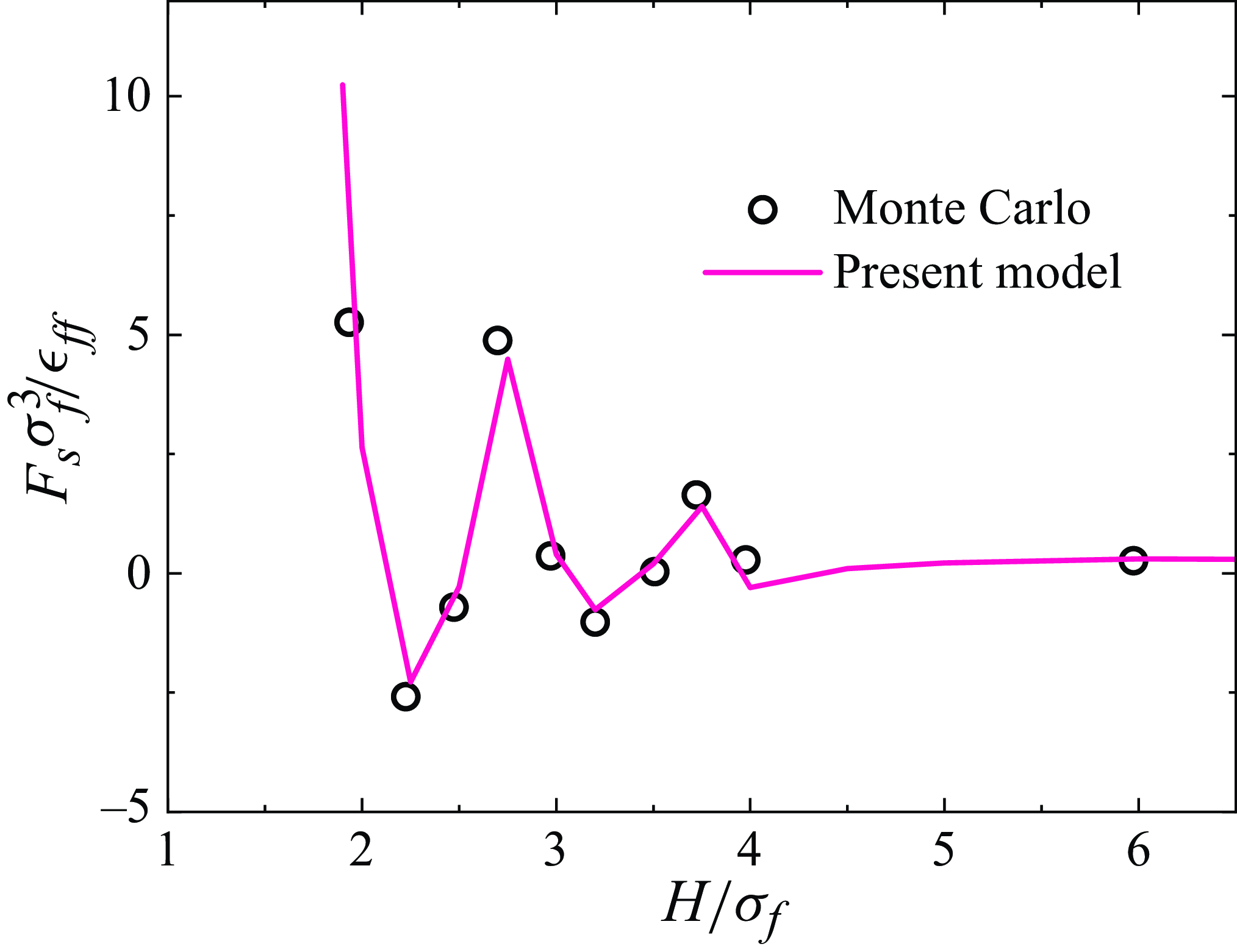
As illustrated in figure 3, the solvation force oscillates with increasing confinement and converges to the bulk pressure
 $p_b$
as the confinement space
 $H$
becomes sufficiently large. Our molecular kinetic model reproduces this oscillatory behaviour, as observed in the Monte Carlo simulations (Snook & van Megen Reference Snook and van Megen1980), confirming the appropriateness of the present molecular kinetic model and the way the hydrodynamic wall is determined. Therefore, the hydrodynamic wall location can be approximately chosen at
 $h=H_{ex}$
, which means that the term
 $Q_{\textit{fs}}^{ex}$
can be neglected in the hydrodynamic bulk flow region (
 $h\gt H_{ex}$
) when modelling fluid–surface interactions.
Oscillation of the solvation force compared with the Monte Carlo simulations (Snook & van Megen Reference Snook and van Megen1980). The following parameters are used: average number density
 $n=0.5925\sigma _f^{-3}$
; temperature
 $T=1.2\epsilon _{\textit{ff}}/k_B$
;
 $\epsilon _{ss}=\epsilon _{\textit{ff}}$
.

2.2.2. Fluid–surface collisions
To model the collision term
 $Q_{\textit{fs}}^0$
, which describes the momentum and energy exchanges between fluids and solids during molecular collisions, we assume that solid molecules remain in Maxwellian equilibrium (Frezzotti & Gibelli Reference Frezzotti and Gibelli2008; Aoki, Giovangigli & Kosuge Reference Aoki, Giovangigli and Kosuge2022), unaffected by fluid–solid collisions due to their strong rigidity, as depicted in figure 1(c). Given that the rates of momentum and energy transfer between fluids and solid surfaces differ (Cercignani Reference Cercignani1988; Woods Reference Woods1993; Struchtrup Reference Struchtrup2013), we introduce a total energy distribution function
 $g=0.5|\boldsymbol{\xi }|^2f$
. Thus,
 $Q_{\textit{fs}}^0$
for momentum (
 $Q_{\textit{fs}}^{m}$
) and energy (
 $Q_{\textit{fs}}^{e}$
) can be modelled separately, each by a relaxation process (Beenakker, Borman & Krylov Reference Beenakker, Borman and Krylov1994; Aoki et al. Reference Aoki, Giovangigli and Kosuge2022),
 \begin{align} Q_{\textit{fs}}^{m} & = -\tau _{m}^{-1} \left (f-f_w^{eq}\right ), \end{align}
 \begin{align} Q_{\textit{fs}}^{e} & = -\tau _{e}^{-1} \left (g-g_w^{eq}\right ), \end{align}
where
 $\tau _m$
and
 $\tau _e$
represent the relaxation times of momentum and energy, which quantify the exchange rates of momentum and energy between the fluid and the solid. These exchanges occur only when fluid molecules are in close contact with the solid surface, so both
 $\tau _m$
and
 $\tau _e$
take finite values at
 $h=H_{ex}$
. Away from the surface, where there is no momentum or energy exchange between the fluid and the solid, these relaxation times effectively tend to infinity. Given this physical interpretation,
 $\tau _m$
and
 $\tau _e$
only play roles at
 $h=H_{ex}$
, as the infinite relaxation at other places does not change the fluid dynamics. In this regard, the collision terms
 $Q_{\textit{fs}}^m$
and
 $Q_{\textit{fs}}^e$
act as effective boundary conditions at
 $h=H_{ex}$
and their influence is localised to the solid surface. Meanwhile, the solid Maxwellian can be written as
 \begin{align} f_w^{eq} & = n_w (2\pi RT_w)^{-\frac {3}{2}}\exp \left (-\frac {|\boldsymbol{\xi } - \boldsymbol{u}_w|^2}{2RT_w}\right ), \end{align}
 \begin{align} g_w^{eq} & = 0.5|\boldsymbol{\xi }|^2f_w^{eq}, \end{align}
where
 $n_w$
is the fluid density at the hydrodynamic wall, and
 $\boldsymbol{u}_w$
is the moving velocity of the surface. Since no fluid penetrates the solid, zero mass flux is achieved at
 $h=H_{ex}$
.
3. Molecular kinetic model
By appropriately modelling fluid–fluid and fluid–surface interactions, the transport equations governing the hydrodynamic flow field (
 $h \geqslant H_{ex}$
) of NCFs can correspondingly be expressed as
 \begin{equation} \left . \begin{split} &D_t f =Q_{\textit{ff}} +Q_{\textit{fs}}^{lg} + Q_{\textit{fs}}^m, \\ &D_t g =0.5|\boldsymbol{\xi }|^2 (Q_{\textit{ff}}+Q_{\textit{fs}}^{lg}) + Q_{\textit{fs}}^e. \end{split}\right \} \end{equation}
Physically,
 $Q_{\textit{fs}}^{m}$
and
 $Q_{\textit{fs}}^{e}$
drive the momentum (
 $f$
) and energy (
 $g$
) distribution functions towards the wall Maxwellian
 $f_w^{eq}$
and
 $g_w^{eq}$
via fluid–solid molecular collisions. This approach eliminates the need for boundary conditions in fluid flows, which have been challenging to define for strongly inhomogeneous fluids. During fluid–surface collisions, only the temporal evolution of distribution functions is considered, as the spatial advection term vanishes due to the fixed position of the hydrodynamic wall. As a result,
 $Q_{\textit{fs}}^{m}$
and
 $Q_{\textit{fs}}^{e}$
can be singled out from the molecular kinetic model (3.1) and expressed separately as
 \begin{align}& \partial _t f =-\tau _m^{-1}(f-f_w^{eq}), \end{align}
 \begin{align}&\, \partial _t g =-\tau _e^{-1}(g-g_w^{eq}). \end{align}
The fluid–solid collisions alter the distribution functions of incoming fluid molecules that collide with the surface. Introducing the characteristic time
 $\bar {t}_{\textit{fs}}$
for fluid–surface collisions, the relationship between precollision and postcollision distribution functions can be given by
 \begin{align} & f(\boldsymbol{\xi }_t, \xi _n)- f(\boldsymbol{\xi }_t, -\xi _n)=-\omega _m\left [f(\boldsymbol{\xi }_t, -\xi _n) - f_w^{eq}\right ], \end{align}
 \begin{align} &\,\, g(\boldsymbol{\xi }_t, \xi _n)- g(\boldsymbol{\xi }_t, -\xi _n)=-\omega _e \left [g(\boldsymbol{\xi }_t, -\xi _n) - g_w^{eq}\right ]. \end{align}
Here,
 $-\xi _n$
and
 $\xi _n$
denote the normal velocities of incoming and outgoing molecules, while
 $\boldsymbol{\xi }_t$
represents the tangential velocity component. The momentum and energy accommodation coefficients
 $\omega _m$
and
 $\omega _e$
measure the momentum and energy transfer rates between the fluid and the solid, which are written as
 \begin{equation} \omega _m=\left \{ \begin{split} \frac {\bar {t}_{\textit{fs}}}{\tau _m},\,\,\,h=H_{ex}, \\ 0,\,\,\,\text{otherwise}, \end{split}\right . \quad \text{and}\quad \omega _e=\left \{ \begin{split} \frac {\bar {t}_{\textit{fs}}}{\tau _e},\,\,\,h=H_{ex}, \\ 0,\,\,\,\text{otherwise}, \end{split}\right . \end{equation}
respectively. These coefficients can be determined experimentally (Ewart et al. Reference Ewart, Perrier, Graur and Méolans2007; Brancher et al. Reference Brancher, Johansson, Perrier and Graur2021), through MD simulations (Yamaguchi, Matsuda & Niimi Reference Yamaguchi, Matsuda and Niimi2017; Han et al. Reference Han, Liu, Li, Zhang and Chen2022; Chen et al. Reference Chen, Gibelli, Li and Borg2023) or via theoretical calculations (Logan & Stickney Reference Logan and Stickney1966; Iftimia & Manson Reference Iftimia and Manson2001).
The conserved variables – fluid density, velocity and energy – are calculated as
 \begin{equation} [\rho , \rho \boldsymbol{u}, \rho E]=m\int \left [f, \boldsymbol{\xi }f, g\right ]{\rm d}\boldsymbol{\xi }, \end{equation}
where
 $\rho =mn$
is the fluid density, and
 $\rho E=(3\rho RT+ \rho |\boldsymbol u|^2)/2$
is the total energy, from which the temperature
 $T$
can be obtained.
It is noted that the expression
 $g=0.5|\boldsymbol \xi |^2 f$
is introduced as an auxiliary function to derive the evolution equation for energy (
 $g$
) based on the evolution of mass/momentum (
 $f$
). During the evolution process,
 $f$
and
 $g$
are not strictly dependent on each other. This is because momentum and energy transfer between the fluid and the solid occurs at a different rate, leading to different relaxation behaviours for mass/momentum and energy. As a result, the relationship
 $g=0.5|\boldsymbol \xi |^2f$
does not hold dynamically. In our molecular kinetic model, the density and velocity are calculated from the velocity distribution function
 $f$
, while the temperature is computed from the energy distribution function
 $g$
. While these calculations are performed separately, the macroscopic variables (velocity and temperature) remain coupled through the local Maxwellian distribution function (2.4c
) and transport coefficients (e.g. viscosity and thermal conductivity). The advantage of introducing the energy distribution function
 $g$
is that it allows independent control of momentum and energy exchange rates between fluids and solids, reflecting their distinct underlying physics.
Through the Chapman–Enskog expansion (Chapman & Cowling Reference Chapman and Cowling1990), we recover the following hydrodynamic equations expressed under the Einstein summation convention:
 \begin{align} \partial _t \rho + \partial _i (\rho u_i)=0, \notag \\ \partial _t (\rho u_i)+\partial _j[p\delta _{ij}-\Pi _{ij}-K_{ij}+\rho u_i u_j]-\rho a_i=0, \notag \\ \partial _t (\rho E)+\partial _j[Q_j+ p\delta _{ij}u_i-(\Pi _{ij}+K_{ij})u_i+\rho E u_j ]-\rho a_i u_i=0, \end{align}
where
 $\delta _{ij}$
is the Kronecker delta function,
 $\boldsymbol{a}=\boldsymbol{a}_e -\nabla {\phi }_{\textit{fs}}^{lg}$
is the total acceleration arising from the external force and fluid–surface interactions and
 $K_{ij}$
is the Korteweg stress tensor (Anderson, McFadden & Wheeler Reference Anderson, McFadden and Wheeler1998), written as
 \begin{equation} K_{ij}=-\frac {1}{6}\int _{|\boldsymbol{r}|\gt \sigma _f}|\boldsymbol{r}|^2\phi _{att}(|\boldsymbol{r}|)\mathrm{d}\boldsymbol{r} \left [\left (n\partial _i\partial _in+\frac {1}{2}|\partial _in|^2\right )\delta _{ij}-\partial _in\partial _jn\right ]. \end{equation}
The pressure
 $p$
is expressed as
 \begin{align} p & = p_0+p_c+p_a, \end{align}
 \begin{align} p_c & = n^2V_0\chi k_BT, \end{align}
 \begin{align} p_a & = \frac {1}{2} n^2\int _{|\boldsymbol{r}|\gt \sigma _f} \phi _{att}(|\boldsymbol{r}|)\mathrm{d}\boldsymbol{r}, \end{align}
with
 $p_c$
accounting for the collisional transfer of momentum and energy and
 $p_a$
for the intermolecular attraction. Meanwhile, the stress tensor and heat flux are expressed as
 \begin{align} \Pi _{ij}&=nk_BT\tau _f\left [1+\frac {2}{5}\bar {n}V_0\chi (\bar {n})\right ] \left [(\partial _i u_j+\partial _j u_i)-\frac {2}{3}\partial _k u_k\delta _{ij}\right ], \notag \\ Q_j&=-c_p\frac {nk_BT\tau _f}{Pr }\left [1+\frac {3}{5}\bar {n}V_0\chi (\bar {n})\right ]\partial _jT, \end{align}
where
 $c_p=2.5R$
represents the fluid specific heat at a constant pressure. By comparing
 $\Pi _{ij}$
and
 $Q_j$
with Newton’s law of viscosity and Fourier’s law of thermal conduction, respectively, we determine the relaxation time
 $\tau _f$
and Prandtl number (
 $Pr$
) as
 \begin{align} \tau _f(n, \bar {n})&= \frac {\mu (n, \bar {n})}{p_0(n)\left [1+\frac {2}{5}\bar {n}V_0\chi (\bar {n})\right ]},\notag \\ Pr (n,\bar {n})&=\frac {c_p\mu (n, \bar {n})}{\kappa (n,\bar {n})} \frac {1+\frac {3}{5}\bar {n}V_0\chi (\bar {n})}{1+\frac {2}{5}\bar {n}V_0\chi (\bar {n})}, \end{align}
where
 $\mu$
and
 $\kappa$
are the fluid viscosity and thermal conductivity, respectively. These transport coefficients can be determined via equilibrium MD simulations as reported in Bhadauria et al. (Reference Bhadauria, Sanghi and Aluru2015) and Bhadauria & Aluru (Reference Bhadauria and Aluru2017), computationally efficient theoretical/empirical formulations such as those reported in Davis, Rice & Sengers (Reference Davis, Rice and Sengers1961), Chung et al. (Reference Chung, Ajlan, Lee and Starling1988) and Chapman & Cowling (Reference Chapman and Cowling1990), or experiments for better accuracy. Here, we use the formulation reported in Chung et al. (Reference Chung, Ajlan, Lee and Starling1988) to determine the transport coefficients, which can reproduce dynamics of van der Waals fluids in good agreement with the MD simulations for LJ fluids (Shan et al. Reference Shan, Su, Gibelli and Zhang2023b
). These transport coefficients depend on both the local density
 $n$
and the local average density
 $\bar {n}$
(Tarazona Reference Tarazona1985; Tarazona et al. Reference Tarazona, Marconi and Evans1987), hence they vary across the confinement space due to fluid inhomogeneities.
Similar to the molecular kinetic model (3.1), equation (3.6) explicitly accounts for strong fluid inhomogeneities and enhanced fluid volume exclusion effects, represented by the force term
 $a_i$
and the collisional transfer term
 $p_c$
, respectively. These terms capture the apparent non-hydrodynamic effects associated with the boundary layer, which are particularly pronounced in NCFs. In contrast, the NSF equations implicitly address both intrinsic non-hydrodynamics effects, such as velocity slip, and apparent non-hydrodynamic effects, like molecular layering structure, through boundary conditions. However, as the apparent non-hydrodynamic effects go beyond the immediate vicinity of the surface, which cannot be described by boundary conditions, the NSF equations become inadequate for describing NCFs.
4. Numerical results and discussion
4.1. Numerical procedures
Both the proposed molecular kinetic model and MD simulations are employed to investigate NCFs, aiming to demonstrate the accuracy and predictive capability of our model. In the MD simulations, the lowest fluid density considered is 60 kg m
 $^{-3}$
, as lower densities introduce significant uncertainty and statistical noise, particularly under strong confinements, e.g. the flows in a 2 nm channel.
We simulate argon confined between two planar solid surfaces with a face-centred-cubic crystal structure. Argon is selected as the working fluid due to its simplicity and well-characterised intermolecular potential (Rahman Reference Rahman1964; Fan et al. Reference Fan, Wu and Wang2020b
). Following established methodologies (Bhadauria et al. Reference Bhadauria, Sanghi and Aluru2015; Bhadauria & Aluru Reference Bhadauria and Aluru2017), our model can potentially be extended to accommodate other fluids and electroosmotic flows. To simulate fluid flows, argon atoms are subjected to an external acceleration rate
 $\boldsymbol{a}_e$
.
For the thermal cases presented in figure 4, the fluid is not thermostatted, allowing for a direct examination of energy evolution in NCFs. In the investigation of the Knudsen minimum phenomenon (figures 5 and 6), an isothermal condition is maintained to better distinguish the effects of fluid–surface interactions and real fluid behaviours on fluid transport properties, where the fluid is governed by the Nosé–Hoover thermostat for stable temperature control, avoiding the need for small external forces that could introduce substantial statistical noise.
The solid atoms are tethered to their lattice sites via a linear spring model, allowing for vibration while maintaining sufficient rigidity to contain the argon atoms. The Nosé–Hoover thermostat is employed to control the temperature of the solid substrate, ensuring thermal stability throughout the simulations. The rough surface in figure 5(a) is achieved by randomly displacing the solid atoms in the
 $y$
direction, with the maximum displacement
 $\Delta y_{max}=0.44$
Å. The confinement space, i.e. the channel height
 $H$
, is defined as the distance between the innermost layer of solid atoms at their equilibrium positions, consistent with the physical wall shown in figure 1(b).
The interactions between argon and solid atoms are modelled using the 12-6 LJ potential with a cutoff distance of 1.3 nm, which is the standard practice in MD simulations. The relevant parameters are
 $\epsilon _{ss}=0.0390$
kcal mol
 $^{-1}$
,
 $\epsilon _{\textit{ff}}=0.2376$
kcal mol
 $^{-1}$
,
 $\sigma _{s}=3.2930$
Å and
 $\sigma _f=3.4039$
Å. For figures 6(c) and 6(d), wettability strengths, quantified by the parameter
 $\epsilon _D = \epsilon _{\textit{fs}}/\epsilon _{\textit{ff}}$
, are varied by multiplying the solid energy parameter
 $\epsilon _{ss}$
by a factor of 2.5 and 0.1, resulting in
 $\epsilon _D=0.641$
and
 $0.128$
, respectively. After achieving equilibrium, the simulations are run with a time step of 0.5 fs for a minimum duration of 5 ns to ensure accurate statistical sampling. The periodic boundary condition is imposed in all the directions. All MD simulations are conducted using the large-scale atomic/molecular massively parallel simulator (Thompson et al. Reference Thompson2022).
The NCFs behaviours in comparison with MD simulations. Panels (a) and (b) are for
 $H=2.5$
nm,
 $T_w=233$
K,
 $|\boldsymbol{a}_e|=2.095\times 10^{12}$
m s
 $^{-2}$
and
 $\rho _{avg}=100$
kg m
 $^{-3}$
;panels (c) and (d) are for
 $H=5.0$
nm,
 $T_w=233$
K,
 $|\boldsymbol{a}_e|=8.382\times 10^{11}$
m s
 $^{-2}$
and
 $\rho _{avg}=500$
kg m
 $^{-3}$
.

(a) Mass flow rates in atomically smooth (
 $\omega _m=0.30$
) and rough (
 $\omega _m=0.82$
) channels. (b) Contributions of real fluid effects and fluid–surface interactions for flows in perfectly rough channels, i.e.
 $\omega _m=1.0$
.

The proposed molecular kinetic model is solved using the discrete unified gas kinetic scheme (Guo et al. Reference Guo, Xu and Wang2013, Reference Guo, Wang and Xu2015; Zhang et al. Reference Zhang, Zhu, Wang and Guo2018), which can simulate strongly inhomogeneous fluid flows (Shan et al. Reference Shan, Wang, Zhang and Guo2020). All the length and energy parameters used in the kinetic model, including
 $\sigma _f$
,
 $\sigma _s$
,
 $\epsilon _{\textit{ff}}$
and
 $\epsilon _{ss}$
, are consistent with those employed in MD simulations for meaningful comparisons.
The accommodation coefficients in our molecular kinetic model are flow system dependent, meaning that once the types of solid and fluid are specified, these coefficients remain constant for a broad range of density, velocity and confinement, if the temperature variation is small. To determine their values, we perform MD simulations and extract velocity and temperature profiles. We then fit these profiles using our molecular kinetic model to obtain the accommodation coefficients. Once determined, these values can be applied to other configurations involving the same fluid–solid system.
Temperature and wettability effects on the mass flow rate. In (a) and (b), the fluid–surface accommodation coefficients are
 $\omega _m=0.53$
,
 $0.30$
and
 $0.23$
for
 $T=183$
K,
 $283$
K and
 $383$
K, respectively. In (c) and (d), the system temperature
 $T=283$
K, and the fluid–surface accommodation coefficients are
 $\omega _m=0.49$
,
 $0.30$
and
 $0.18$
for
 $\epsilon _D=0.641$
, 0.405 and 0.128, respectively.

4.2. Features of NCFs
For force-driven channel flows shown by figure 1(f), figure 4(a,b) presents the density, velocity and temperature profiles for
 $H=2.5$
nm,
 $T_w=233$
K, external acceleration
 $|\boldsymbol{a}_e|=2.095\times 10^{12}$
m s
 $^{-2}$
in the flow direction and an average density
 $\rho _{avg}=100$
kg m
 $^{-3}$
. The fluid–surface accommodation coefficients,
 $\omega _m=0.32$
and
 $\omega _e=0.10$
, are determined through independent MD simulations with the same LJ parameters. The results of the present molecular kinetic model align well with the MD simulation data, as shown in figure 4. A pronounced density peak, indicating fluid adsorption due to fluid–surface interactions, is observed near the solid surface and rapidly diminishes with distance. This layering structure of NCFs, though frequently reported in MD simulations, has been largely overlooked by previous kinetic models (Li, Xu & Li Reference Li, Xu and Li2010; Barisik & Beskok Reference Barisik and Beskok2011) due to their oversimplification of fluid–surface interactions.
Momentum and energy transfer between the fluid and solid molecules is modulated by the local density of the adsorbed fluid, which depends on the fluid–surface interaction strength. Notably, the present kinetic model captures non-hydrodynamic effects at the fluid–solid interface, predicting a slip velocity of
 $u_s\simeq 42$
m s
 $^{-1}$
and a temperature jump of
 $T_j\simeq 11.3$
K, both closely matching MD simulation results. The model also accounts for viscous heating effects, as shown in the inset of figure 4(b), though this temperature distribution is less discernible in MD simulations due to thermal fluctuations.
Figure 4(c,d) displays fluid behaviours at
 $H=5.0$
nm,
 $T_w=233$
K,
 $|\boldsymbol{a}_e|=8.382\times 10^{11}$
m s
 $^{-2}$
and
 $\rho _{avg}=500$
kg m
 $^{-3}$
. Once again, the present molecular kinetic model demonstrates excellent agreement with MD data, showcasing its modelling capability for NCFs across a broad range of densities.
Traditional boundary conditions attempt to encapsulate both the intrinsic and apparent non-hydrodynamic effects arising from fluid–solid interactions. However, the thickness of the adsorbed layers in NCFs, which varies with the solid type and thermodynamic conditions, is non-negligible (Hadjiconstantinou Reference Hadjiconstantinou2024). Therefore, the adsorbed layer effects cannot be captured by boundary conditions. Our molecular kinetic model consistently considers molecular interactions between fluid and solid surface molecules, integrating both intrinsic and apparent interfacial dynamics within a unified transport equation and thus more suitable for predicting NCFs behaviours.
4.3. Knudsen minimum
In the Poiseuille flow of a rarefied gas, the mass flow rate, defined as
 \begin{equation} Q_n=u_m\int \frac {\rho u}{\rho _{avg}|\boldsymbol{a}_e|H^2}\mathrm{d}y, \end{equation}
typically exhibits a characteristic minimum as the Knudsen number varies, a phenomenon known as the Knudsen minimum (Cercignani Reference Cercignani1988). This behaviour arises from the interplay between viscous dissipation within the fluid and velocity slip at the fluid–solid interface (Wu et al. Reference Wu, Liu, Reese and Zhang2016; Sheng et al. Reference Shan, Wang, Zhang and Guo2020). The Knudsen number is defined as
 \begin{equation} Kn=m[\sqrt {2} \rho _{avg} \pi \sigma _f^2\chi (\rho _{avg}) H]^{-1}. \end{equation}
As the fluid density increases, the Knudsen minimum disappears. This behaviour was first reported by Guo, Zhao & Shi (Reference Guo, Zhao and Shi2006) for confined fluids and later investigated for dense fluids (Wu et al. Reference Wu, Liu, Reese and Zhang2016; Corral-Casas et al. Reference Corral-Casas, Li, Borg and Gibelli2022). However, these studies do not fully account for the complex interactions between fluid and vibrating solid molecules at the interface.
Figure 5(a) illustrates the mass flow rate at
 $T_w=283$
K, where we focus on isothermal systems with the momentum accommodation coefficient
 $\omega _m = 0.30$
and
 $0.82$
for the smooth and rough surfaces, respectively. The predicted mass flow rates show satisfactory agreement with MD simulations across a wide range of Kn, from 0.039–1.025. However, obtaining MD data for Kn
 ${\gt } 1.025$
is challenging due to significant thermal fluctuations. An increase in the fluid–solid accommodation coefficient causes a transition from specular to diffuse reflections, as shown in figure 1(d,e). Therefore, a larger accommodation coefficient normally corresponds to a more efficient momentum transfer, representing a rougher channel surface. Comparing results obtained for different accommodation coefficients (
 $\omega _m=0.30$
and
 $0.82$
) highlights the enhancement of the mass flow rate resulting from specular reflections in nanoscale flows confined by atomically smooth surfaces. This enhancement reflects the rapid mass transport enhanced by specular reflection, as observed in MD simulations and experimental studies (Keerthi et al. Reference Keerthi2018; Qian, Wu & Wang Reference Qian, Wu and Wang2023). Note, as the flow velocity in nanochannels is usually small, the thermal dissipation may be neglected, which leads to simplification of the model, i.e. the evolution of energy distribution function in (3.1), can be ignored.
Unlike the classical Knudsen minimum, typically observed at Kn
 $\sim 1.0$
, our results reveal a terrace regime for
 $0.2\lt$
Kn
 ${\lt } 1.0$
in a 2 nm channel. This terrace-like behaviour indicates a balanced competition between the decreasing rate of viscous dissipation and the increasing rate of surface flow resistance within this range.
To elucidate the impact of fluid–surface interactions and real fluid effects on NCFs behaviours, we single out their respective contributions from the present molecular kinetic model. When
 $H_{att} \ll H$
, the fluid–surface interaction term
 $Q_{\textit{fs}}^{lg}$
becomes negligible and the hydrodynamic wall coincides with the physical boundary. In this limit, our model simplifies to the Enskog–Vlasov (EV) model (Shan et al. Reference Shan, Su, Gibelli and Zhang2023b
). For consistency, we use
 $\omega _m=1.0$
in our model and apply the diffuse boundary condition in the reduced EV model. The difference in predictions between the present and EV models highlights the impact of fluid–surface interactions, which uniformly reduce the mass flow rate across all flow regimes by shortening the effective flow path and thereby increasing flow resistance. Although this enhanced resistance is a characteristic of NCFs, the overall flow rate can still be significantly increased by the large velocity slip occurring at smooth solid surfaces, an effect driven by the specular reflection of fluid molecules (Lichter et al. Reference Lichter, Martini, Snurr and Wang2007; Martini et al. Reference Martini, Roxin, Snurr, Wang and Lichter2008a
; Keerthi et al. Reference Keerthi2018), as quantified in figure 5(a).
At low densities, the terms
 $Q_{\textit{ff}}^{lg}$
and
 $Q_{\textit{ff}}^1$
describing real fluid effects can be neglected. Therefore, the EV model reduces further to the Shakhov model equation for a perfect gas. The simulation results are in good agreement with the solution of the Boltzmann equation (Ohwada, Sone & Aoki Reference Ohwada, Sone and Aoki1989), as shown in figure 5(b). Real fluid effects, including the finite volume of fluid molecules and intermolecular attractions, reduce the mass flow rate, especially in the cases with Kn
 ${\lt } 0.1$
and strong confinement (see figure 5). In contrast, when Kn
 ${\gt } 1.0$
, the flow rate is only marginally affected by real fluid effects due to the insignificance of interactions between fluid molecules.
Figures 6(a) and 6(b) demonstrate that higher temperatures result in more pronounced mass flow rates, a behaviour that contrasts with predictions from the Boltzmann equation, where the temperature has no effect on the flow rate. This discrepancy arises because (i) real fluid viscosity deviates from the relation
 $\mu \propto T^{\frac {1}{2}}$
for a perfect gas (Shan et al. Reference Shan, Su, Gibelli and Zhang2023b
), and (ii) the fluid–surface accommodation rates vary with temperature (Cercignani Reference Cercignani1988). Notably, while the Knudsen minimum disappears at high temperatures (283 and 383 K) in 2 nm nanochannels, it re-emerges at a lower temperature (183 K), where the convective flow is enhanced and the velocity slip is suppressed. This finding reinforces the explanation of how the Knudsen minimum vanishes for confined dense/real fluids.
Fluid adsorption is macroscopically governed by surface wettability (Fan et al. Reference Fan, Wu and Wang2020a
) and quantified by the contact angle, which is directly related to the fluid–solid interaction strength
 $\epsilon _D$
(Barrat & Bocquet Reference Barrat and Bocquet1999; Perumanath et al. Reference Perumanath, Chubynsky, Pillai, Borg and Sprittles2023). As shown in figures 6(c) and 6(d), as
 $\epsilon _D$
decreases, the mass flow rate increases significantly, reflecting the transition from hydrophilic to hydrophobic surface conditions. Under hydrophobic conditions, the lower fluid density near the surface and weaker fluid–surface attraction result in larger velocity slips, thereby leading to more pronounced flow rates. Therefore, our model captures composition-dependent non-hydrodynamic effects observed in MD simulations (Martini et al. Reference Martini, Roxin, Snurr, Wang and Lichter2008b
; Hadjiconstantinou Reference Hadjiconstantinou2024).
5. Conclusion
In summary, we have developed a novel molecular kinetic model for NCFs that accurately captures the complex interactions between fluid and vibrating solid molecules, accounting for strong fluid inhomogeneities and non-hydrodynamic effects of both dilute and dense fluids confined in nanospaces. To accurately describe nanoconfined flows, it is required to take both fluid–fluid and fluid–surface interactions into account in the transport equation. Fluid–fluid interactions give rise to real fluid effects, while fluid–surface interactions influence adsorption, slip velocity, temperature jump and fluid inhomogeneity. It is shown that surface smoothness and fluid adsorption significantly affect mass flow rates in nanoconfined flows, which has been mostly overlooked in previous studies. As a result, conventional models (e.g. the Navier–Stokes or Boltzmann equations) fail to accurately reproduce MD results in nanoconfined flows.
Validated by MD simulations, our model marks a significant advance in the theoretical modelling of NCFs, providing a unified framework that bridges microscale and macroscale dynamics. With wettability effects inherently embedded (see figure 6 c,d), the model captures essential molecular physics and is ideally suited for studying nanoscale phenomena such as droplet-bubble dynamics (Li et al. Reference Li, Su, Shan, Li, Gibelli and Zhang2024b ), dynamic wetting (Sprittles Reference Sprittles2015) and liquid–vapour evaporation (Sadr et al. Reference Sadr, Pfeiffer and Gorji2021; Struchtrup & Frezzotti Reference Struchtrup and Frezzotti2022).
It is worth noting that a common approach in the literature to account for nanoscale effects involves adding correction functions to the continuum theory (Chubynsky et al. Reference Chubynsky, Belousov, Lockerby and Sprittles2020; Fan et al. Reference Fan, Wu and Wang2020a ; Perumanath et al. Reference Perumanath, Chubynsky, Pillai, Borg and Sprittles2023), referred to as top-down modelling. In contrast to top-down models that prescribe the velocity or temperature slip lengths a priori as boundary conditions, our model predicts these quantities by microscopically integrating the physical mechanisms of real fluid effects and fluid–surface interactions within the transport equation, representing a bottom-up modelling strategy. While the slip length in the top-down models is dependent on density and confinement, the fluid–surface accommodation coefficient in our model is independent of these parameters.
Acknowledgements
B.S. acknowledges the support given by the Alexander von Humboldt Foundation, Germany.
Funding
This work was supported by the National Natural Science Foundation of China (grant no. 12472290).
Declaration of interests
The authors declare no competing interests.