
I. INTRODUCTION
Materials submitted to particles (neutron, ion, and electron) irradiation undergo a multitude of complex chemical and structural changes at length scale spanning the atomistic to the macroscopic regimes from few picoseconds to years. Predicting mechanical and thermal properties of these materials is difficult as irradiation drives the system away from equilibrium. The aging of these materials under irradiation has thus been an ongoing field of research for several decades. Since it can induce variation of the local composition at the atomic scale, irradiation offers the opportunity to overcome the thermodynamic phase diagram manufacturing alloys with unexpected composition fluctuations at the mesoscopic scale. On an academic point of view, materials under irradiation may be toy models to study the formation and the stability of systems maintained far from equilibrium. Varying the control parameters (temperature and particle flux), experimentalists and theoreticians can validate different approaches for understanding systems maintained far from equilibrium.
Different simulation techniques were developed over the past decades to predict the longtime microstructural evolution of solids under irradiation. Over the past three decades, classical molecular dynamics (MD) methods were extensively applied to estimate primary damage production in materials (alloys and ceramics) submitted to radiation damage. This atomistic simulation method allows describing the first stage of radiation damage in materials. However, the time scale of the simulation (few picoseconds) makes it unavailable to discuss long-term aging of materials under irradiation over the diffusive time scale (few microseconds) that controls the microstructure formation. Usual approaches to model precipitates generated under irradiation (defects cavities, secondary phases, and gas bubbles) during the aging of materials at the mesoscale, i.e., over few hundreds of nanometers, are based on the rate theory (RT). In the RT formalism, classical nucleation theory is applied to determine the spatially averaged vacancy and interstitial and solute populations.
In this mean field approximation, the underlying microstructural features (nature of extended defects) are assumed frozen and the spatial correlations between defects is neglected. To overcome this last limitation, kinetic Monte-Carlo (KMC) methods were developed enabling the spatial resolution of individual class of defects (point defect, dislocations, cavities…). This simulation tool, very efficient at low temperature when the point defect concentration is low, can be extended to include many dynamics acting in parallel. The first limitation of the KMC technique is the simulation cell size which dictates the observable cluster density. The second and the most restrictive limitation of this method is due to the fact that all different dynamics associated with extended defect formation must be added by hand. Within such an approximation, the evolution of a microstructure depends on a finite number of predefined defects. Their jump frequencies and reaction activation energies are input parameters and must be computed from other techniques (for instance ab initio calculations). Another severe limitation of this technique comes from the fact that lattice relaxations induced by electric fields (for insulators) and/or elastic fields (for metals) cannot be handled due to the limitation of the size of the simulation boxes.
Continuum methods’ phase field (PF) method is based on a mean field theory describing the evolution of the microstructure by continuum fields evolving in space and time. This approach can overcome the KMC limitation enabling to introduce long range fields.
General reviews of applications of the PF method to radiation to compute long time radiation-induced microstructures are available in the literature. Reference Millet and Tonks1,Reference Li, Hu and Stan2 Due to these recent developments and its flexible applicability, PF seems to have a large potential to impact the radiation material science community. PF models were successfully applied to discuss cavity formation and gas bubbles produced under irradiation. Reference Hu and Lu3–Reference Hu, Burkes, Lavender, Senor, Setyawan and Xu5 The main advantage of the PF approach lies in the handling of point defect fields. All spatial information on the microstructure is contained in these fields taking into account long range interaction like elastic or/and electric fields.
Concentration Reference Khatchaturyan6 (or more largely order parameter (OP) Reference Tolédano and Dmitriev7 ) fields resulting from a coarse grained average of the atomic occupation over a discrete underlying rigid lattice simulate only the long range order (LRO) of the systems like RT simulations. However, correlations between these mean values are introduced “by hand” via differential operators in a free energy functional (the so called Ginzburg term Reference Tolédano and Dmitriev7 ) allowing local fluctuations very few nanometers of the OPs. The energy cost associated to this large variation is directly related with the formations of interfaces. The main interest of this approach is its ability in comparison with atomistic simulations to take into account in-homogeneous local long range fields like strain fields produced during the microstructure evolution. In the PF approach, steady states result from a minimization of an effective free energy. However, the main limitation of such an approach is due to the absence of clear coarse grained procedures. Reference Elder, Katakowski, Haataja and Grant8 This fact leads the study of the relative stability of different minima of the effective free energy difficult, i.e., possible steady states.
Although continuous approximations suffer from some limitations, they offer the unique opportunity to discuss self organization in condensed matter at equilibrium and far from equilibrium. Reference Ghoniem and Walgraef9–Reference Van Kampen11 This work discusses the application of different methods to rationalize and explain patterning observed in some materials during irradiation. From examples extracted from the RT formalism, the first part of this paper is devoted to the presentation of the main methods used to discuss patterning (phase portrait, local stability, amplitude equations, and associated instabilities). The second part of this paper discusses radiation-induced patterning modeled within the PF approximation.
II. RADIATION-INDUCED CLUSTERING
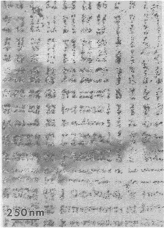
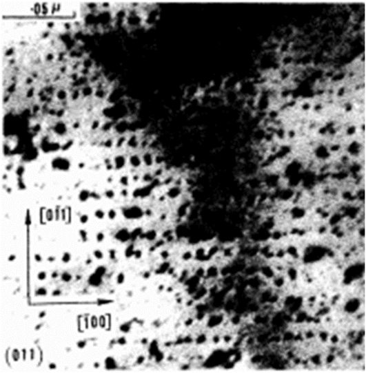
During irradiation, neutrons, ions, or electrons slow down in matter changing the isotopic composition of the medium (for neutrons), modifying the electron landscape (swift heavy ions), and setting in motion atoms at rest. All these different mechanisms will produce many point defects (vacancies, interstitials, and antisite defects) and extended defects (dumbbells, dislocations, cavities, and precipitates). The atomic fractions of these defects are much larger than those (if they are) produced at equilibrium leading to the formation of unusual microstructures and even new patterns. Even if the mechanism associated with the formation of defects in the track of swift heavy ions (above 1 keV/amu) is far from being clearly understood, the processes associated with defects production induced by low energy deposition (below 1 keV/amu) are well identified at least in metals and alloys (for a discussion on these atomistic models see Ref. Reference Simeone, Costantini, Luneville, Desgranges, Trocellier and Garcia12). Point defects (mainly vacancies and interstitials) are produced in highly perturbed areas named “displacement cascades” over a time scale of few tens of picoseconds and a space scale of few nanometers [the characteristic size of a displacement cascade induced by low energy ions (below 1 MeV)]. The theory of damage production by displacement cascades is now well understood and efficient atomistic simulations (mainly based on the MD techniques) are now available to compute defect production rates. However, such atomistic simulations are enabled to describe unusual patterns Reference Krishan13 observed over large space and time scales in irradiated materials. As an example of the unexpected microstructure, Fig. 1 displays the formation of periodic arrays of vacancy loops in pure copper irradiated with 1 MeV H ions at room temperature. Reference Jager, Erhart, Schilling, Dworschak, Gadalla and Tsukuda14,Reference Jager and Trinkaus15
Periodic array of the planar 001 wall of dislocations in Cu irradiated in pure Cu at 0.65 dPa @ RT. Reprinted from Ref. Reference Jager and Trinkaus15, Copyright 4218671135868, with permission from Elsevier.

By analogy with patterns observed in many fields of physics, Reference Nicolis and Prigogine10,Reference Van Kampen11 many studies were devoted to model different reaction diffusion processes able to create such unusual patterns. Reference Krishan13
A. Birth and death process
Within the cluster dynamics (CD) approximation, defects are treated as lattice gas. These defects produced by athermal processes will diffuse in crystalline solids and agglomerate in clusters over a time scale
 $\tau \propto {{\rm{e}}^{{{{E_{\rm{a}}}} \over {kT}}}} \approx {10^{ - 6}}{\rm{s}}$
(where E
a the activation energy varies from few hundreds of MeV to few eV) over a time scale five orders of magnitude larger the production rate in displacement cascades (few picoseconds), and a space scale defined by the mean distance between different sinks and roughly equal to few hundreds of nanometers, i.e., two orders of magnitude larger than the displacement cascade characteristic size. When defects start to agglomerate into clusters, the size of each cluster grows and shrinks by a process of accretion and emission, controlled by the local concentration of point defects in the neighborhood of the cluster.
Reference Karlin and Taylor16
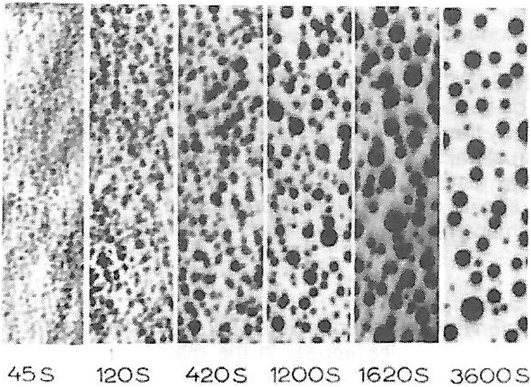
Figure 2 displays the coarsening kinetics of lead particles under electron irradiation.
Coagulation kinetics of Pb particles produced by 125 keV electron irradiation (at 673 K with a flux of 4.81018 cm−2/s) in lead glass. Reprinted with permission from Ref. Reference Biron50, Orsay university.

An appropriate framework for describing such events is the theory of stochastic processes Reference Nicolis and Prigogine10,Reference Van Kampen11 for which the cluster size appears to be a random variable. The decoupling of time and space scales allows applying the master equation (ME) formalism to discuss the microstructure formation in crystalline solids induced by vacancies and interstitials. This description is extensively used to discuss a large class of phenomena like chemical reactions. Reference Nicolis and Prigogine10,Reference Gillespie17 The ME refers to a Markov process in which state transitions can occur only between neighboring states (i → i + 1 or i → i − 1). Within the CD approximation, Reference Ghoniem and Walgraef9 one assumes in many cases that only monomers (vacancy, interstitial, and gas fission resulting from transmutation) migrate. The probability P(n, t) to create a cluster of size n obeys to the following differential equation for (n ≥ 2):
 $${{{\rm{d}}P\left( {n,t} \right)} \over {{\rm{d}}t}} = {J_{n - 1 \to n}} - {J_{n \to n + 1}}\quad .$$
In this expression, the cluster flux associated with the motion of clusters belonging to a class of size n to the class n + 1 is usually written as J n→n+1 = λ n P(n, t) − μ n+1 P(n + 1, t). In this last expression, λ n is the probability rate (per time unit) for one monomer to be scotched to a cluster of size n and μ n is the probability rate for a monomer to leave a cluster of size n. As atomic clustering in many cases Reference Binder and Stauffer18 is driven by the concentration of monomers (vacancies, interstitials, and gas), the complete distribution of clusters (di-mere, tri-mere…) must be computed. This distribution is given by a coupled hierarchy of these discrete equations. Equation (1) casts as
 $$\eqalign{ {{{\rm{d}}P\left( {n,t} \right)} \over {{\rm{d}}t}} = {\lambda _{n - 1}}P\left( {n - 1,t} \right) + {\mu _{n + 1}}P\left( {n + 1,t} \right) \cr - \left( {{\lambda _n} + {\mu _n}} \right)P\left( {n,t} \right)\quad . \cr}$$
This last equation defines a birth and death (BD) process. Reference Nicolis and Prigogine10,Reference Van Kampen11 The probability rates λ i and μ i are highly nonlinear function of the temperature and the flux as well as the cluster size.
In a pure birth process (λ i = λ; μ i = 0), P(i, t) is given by a Poisson distribution and the variance of the process is equal to its mean value. It results that the cluster distribution modeled by a BD process is determined not only by the average size of clusters 〈iP(i, t)〉 but also by all its higher moments (fluctuations). Fluctuations (second moments, third moments…) are obviously related to the system size and the correlation length over which two parts of the system “feel” each others. The main limitation of modeling cluster formations under irradiation by a BD process is to accurately determine different transition rates. Reference Waite19,Reference Abromeit and Wollenberg20 These reaction rates do not depend on the different moments of the defect concentration but are the function of the defect concentrations.
B. Rate theory
It has been clearly shown Reference Nicolis and Prigogine10 that if λ n and μ n in Eq. (2) follow a Poisson distribution, the cluster size can be computed assuming that λ i and μ i depend only the averaged value of defect concentrations. Such an assumption called the RT approximation Reference Nichols21 is extensively applied to describe chemical reactions. The RT can be understood as a mean filed theory as these transition rates calculated neglecting all fluctuations of defect concentrations. Thus, the time evolution of the population of point defects [vacancy (v), interstitial (i), and sinks like free surface, grain boundaries, or dislocations loops (s)] is dictated by the following “chemical” reactions:
 $${\rm{v}} + {\rm{i}} \to \emptyset \quad,$$
 $${\rm{v}} + {\rm{s}} \to {\rm{s}}\quad,$$
 $${\rm{i}} + {\rm{s}} \to {\rm{s}}\quad .$$
In this approach, the underlying lattice is neglected. Assuming a law of mass action can be applied, the number of λ i and μ i terms can be reduced, leading to a new set of control parameters K. This set of chemical reactions can be mathematically handled by a set of deterministic equations:
 $${{{\rm{d}}{C_{\rm{i}}}} \over {{\rm{d}}t}} = {K_{\rm{i}}} - {K_{{\rm{iv}}}}{C_{\rm{i}}}{C_{\rm{v}}} - {K_{{\rm{is}}}}{C_{\rm{i}}}{C_{\rm{s}}}\quad,$$
 $${{{\rm{d}}{C_{\rm{v}}}} \over {{\rm{d}}t}} = {K_{\rm{v}}} - {K_{{\rm{iv}}}}{C_{\rm{i}}}{C_{\rm{v}}} - {K_{{\rm{vs}}}}{C_{\rm{v}}}{C_{\rm{s}}}\quad,$$
where C i, C v, and C s are interstitial, vacancy, and sink volume concentrations.
Introducing the production rate K
i(v) of free migrating interstitials and vacancies escaping from displacement cascades, these terms can be written as νi(v)σ
d
ϕ, where ϕ is the flux of impinging particles, σ
d
is a displacement cross section
Reference Sigmund and Gras-Marti22
and is an estimation of the displacement cascade formation averaged over all crystalline directions,
Reference Simeone and Luneville23
and νi(v) is an efficiency factor varying from few percents to few tens of percent depending on the temperature and the displacement cascade density.
Reference Kiritani24
Within the effective medium theory framework,
Reference Brailsford and Bullough25
many studies
Reference Dunlop, Rullier-Albenque, Jaouen, Templier and Davenas26
were devoted to calculate vacancy–interstitial recombination
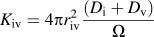 ${K_{{\rm{iv}}}} = 4\pi r_{{\rm{iv}}}^2{{\left( {{D_{\rm{i}}} + {D_{\rm{v}}}} \right)} \over \Omega }$
, where r
iv is the radius capture in which a vacancy and an interstitial recombines and D
i(v) is the thermal diffusion of interstitials (vacancies) in the medium. The term Ω is the atomic volume. The term
 ${K_{{\rm{i}}\left( {\rm{v}} \right){\rm{s}}}} = k_{{\rm{i}}\left( {\rm{v}} \right){\rm{s}}}^2{D_{{\rm{i}}\left( {\rm{v}} \right)}}\left[ {{C_{{\rm{i}}\left( {\rm{v}} \right)}} - C_{{\rm{i}}\left( {\rm{v}} \right)}^{{\rm{eq}}}\left( T \right)} \right]$
, where
 $k_{{\rm{i}}\left( {\rm{v}} \right){\rm{s}}}^{ - 1}$
is a mean free path associated with the diffusion of a point defect to a sink and has the dimension of a length and
 $C_{{\rm{i}}\left( {\rm{v}} \right)}^{{\rm{eq}}}\left( T \right)$
is the equilibrium concentration of point defects in the medium. The temperature appears in the recombination terms assumed to be thermally activated.
Reference Nichols21
The term K
is (K
is respectively) controls the vacancy (interstitial) concentration in the vicinity of a given sink (dislocation line, cavity, bubble…). The effect of the sink strength mediated by the elastic/electric fields governs these terms.
This approach can be extended to study the growth rate of precipitates, dislocation, and voids by adding specific evolution laws. Reference Abromeit and Wollenberg20,Reference Maydet and Russel27
Within this approximation, the nonequilibrium concentration of point defects results from the resolution of a set of p-coupled nonlinear autonomous (the time does not directly appear in their right hand side) differential equations Reference Sizmann28 :
 $${{\dot{\bf U}}} = F\left( {{\bf{U}},T,\phi } \right)\quad,$$
where U is the concentration field vector (C
i, C
v, C
s)
t
. This set of equations typically describes the evolution of dissipative dynamical systems.
Reference Berge, Pomeau and Vidal29
The energy of the incident particles bumping the material is dissipated via the creation of point and extended defects. The flux ϕ and the temperature T can be understood as control parameters in the theory of dynamic systems.
Reference Berge, Pomeau and Vidal29
In the functional F(U, T, ϕ), the physics associated with three main causes of the microstructure formation under radiation damage, i.e., interaction between clusters or loops, fast interstitial migration, and interstitial loops punched out from over pressure gas bubbles must be physically sounded. Modeling these effects implies that many parameters like the bias strengths of bubbles to capture radiation-induced point defects must be known. This is the main difficulty of these approaches.
Reference Li, Hu and Stan2,Reference Hu, Burkes, Lavender, Senor, Setyawan and Xu5
Moreover, finding precise solutions for the equations defining the dynamical system [Eq. (5)] is often hopeless and one prefers to study the long term behavior of solutions. As this system is dissipative, it settles down to steady states defined by all possible attractors in the phase space. The number and the nature (attractive, repulsive…) of these attractors determine the long-term behavior of the system versus the initial conditions and the control parameters (the flux, the temperature, and input parameters like the activation energy). The qualitative evolution of the system can be obtained from the phase portrait of dimension p associated to a set of p autonomous differential equations. The phase portrait results from the direct calculation of the velocity field
 ${{\dot{\bf U}}}$
versus U via Eq. (5). Fortunately, a great deal of insight into the behavior of the system is obtained simply by knowing the sign of the time derivative of each point in the phase portrait.
Reference Somorjai30
This numerical procedure allows us to determine all possible attractors.
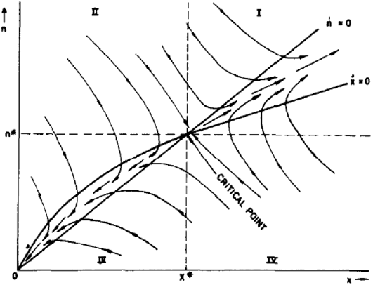
Figure 3 displays a phase portrait for radiation-induced formation of incoherent precipitates. Reference Maydet and Russel27 In this example, the time evolution of coherent precipitates is dictated by two distinct variables, the number of solute atoms n, and the vacancy concentration x. Precipitates with atomic volumes greater than the matrix volume (n > n*) will increase to relieve the local strain energy, and the undersized precipitates (n < n*) associated with smaller atomic volume will vanish. Within the RT approximation, these continuum fields are given by Reference Maydet and Russel27
 $$\dot{x} = {\lambda _{\rm{X}}}\left( {x,n} \right) - {\mu _{\rm{X}}}\left( {x,n} \right)\quad,$$
 $$\dot{n} = {\lambda _{\rm{V}}}\left( {x,n} \right) - {\mu _{\rm{V}}}\left( {x,n} \right) - {\lambda _i}\left( {n,x} \right)\quad,$$
where λX, λV, and λV are accretion rates of solute and they are proportional to the flux, vacancies, and interstitials, respectively. The terms μX and μV can be written as functions of the temperature and the free enthalpy ΔG(n, x). Reference Maydet and Russel27 They are the rate of loss of solutes and vacancies. All the underlying physics describing the radiation-induced precipitation are included in these terms. This set of equation can be written in a concise way by Eq. (5).
2D phase portrait of the number of solute atoms (x) and excess vacancies (n) calculated as the excess between the atomic volume of a host atom and a solute atom in an incoherent precipitate produced under irradiation. Reference Maydet and Russel27 Arrows indicate particle velocities in the (x, n) space. These velocities exhibit different orientations in each quadrant (I to IV). The particle moves into the stable node (0, 0) the saddle critical point (x*, n*). They spiral into the stable focus (non-null real part of the complex conjugate eigenvalues) and circle around the center (null real part of the complex conjugate eigenvalues).

As clearly displayed in Fig. 3, the trajectories of the variables (n, u) are attracted (or repelled by) to different specific points named as attractors in different quadrants (basins of attraction). These points are obviously zeros of F(U, T, ϕ) = 0. This example highlights the interest of the phase portrait to determine the different steady states versus control parameters like the temperature and the irradiation flux.
Different questions naturally appear: how can we define the nature of different possible attractors U 0 leading to distinct steady states and can a change of control parameters induced a bifurcation from one attractor to another one? The next section is devoted to answer such questions.
C. Bifurcation and instability
For dissipative systems, it is possible to define the nature of these different attractors calculating eigenvalues λ j of the first derivative DF(U, T, ϕ) (a p × p matrix) of F(U, T, ϕ) calculated for different U 0 points. As F is a real function, eigenvalues of DF(U, T, ϕ) are real or complex conjugated:
-
(i) A fixed point is called a Node when both eigenvalues are real and of the same sign. The node is stable when the eigenvalues are negative and unstable when they are positive. For the stable node, the eigenvalue(s) with minimal absolute value of the real part is called principle or leading; when the eigenvalues are different, all orbits but two tend to the node along the leading eigen-vector (the picture is reversed for the unstable node);
-
(ii) A fixed point is called a Saddle when eigenvalues are real and of opposite signs. The saddle is always unstable;
-
(iii) A fixed point is called a Focus (sometimes called spiral point) when eigenvalues are complex conjugate; the focus is stable when the eigenvalues have negative real part and unstable when they have positive real part.
It must be noticed that nodes change stability when time is reversed (i.e., when t is replaced by −t), whereas saddles are unstable regardless of the direction of time. Other kinds of fixed points (non hyperbolic ones) can exist. Reference Somorjai30 Obviously, the nature of different fixed points depends on the dimension of the ordinary differential equation set. Increasing the dimension p, various types of hyperbolic attractors can appear. Reference Somorjai30
Since evolution of the system is dictated by nonlinear differential equations [see Eq. (5)], the nature of steady states may evolve for different values of the set of the control parameters (ϕ, T), labeled μ below, leading to bifurcation of different steady states for critical values of μc. A bifurcation leads to an exchange of the stability between two different steady states of the dynamical system. In fact, the system jumps from one attractor to another point attractor. A classification of all possible bifurcations has been dressed by physicists. Reference Cross and Hohenberg31 As an illustration, we consider two types of bifurcation extensively observed in the phase transition community. Reference Tolédano and Dmitriev7 In the 1D system, the time evolution of the OP U during a second order phase transition is given by
 $$\dot{U} = \mu U - {U^3}\quad .$$
Hence, the fixed point is null for μ ≤ 0 and becomes unstable for positive values of μ while nonzero fixed points exist and are stable for positive μ values. The bifurcation is supercritical and known as a pitchfork bifurcation. Introducing a fifth order term U 5 in Eq. (7), it is possible to describe first order phase transition:
 $$\dot{U} = \mu U + \nu {U^3} - {U^5}\quad .$$
The null fixed points stable for
 $\mu \ge {{ - {\nu ^2}} \over 4}$
become unstable leading to a subcritical bifurcation showing a hysteresis as expected for a first order phase transition as displayed in the bifurcation diagram (Fig. 4).
Evolution of the fixed point U
0 versus the control parameter μ in 1D. (a) Displays a supercritical bifurcation and (b) displays a subcritical bifurcation (ν = 2). Full curves are associated with stable solutions and dashed lines define unstable solutions. In the supercritical bifurcation, two opposite stable solutions
 ${U_0} = \sqrt \mu$
exist for μ > 0. The null solution is stable for μ < 0. In the subcritical bifurcation, two distinct points U
0 = 0 and
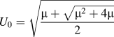 ${U_0} = \sqrt {{{\mu + \sqrt {{\mu ^2} + 4\mu } } \over 2}}$
are stable for
 $- {{{\nu ^2}} \over 4} \le \mu \le 0$
ensuring that two distinct steady states occur for these values of μ. The existence of these two stable points ensures that a hysteresis takes place in this domain.

The stability of a given attractor versus μ can be determined from the amplification rate ω(μ) defined as
 $\det \left( {{{\left. {{{\partial {F_i}\left( {{{\bf{U}}_{\bf{0}}},\mu } \right)} \over {\partial {U_j}}}} \right|}_{{U_0}}} - \omega \left( \mu \right){\delta _{ij}}} \right) = 0$
resulting from the linearization of Eq. (5) in the vicinity of μc. When the real part of ω(μ) vanishes, such a bifurcation is called a subcritical bifurcation diagram. Sometimes, the real part of ω(μ) vanishes but its imaginary part is non-null leading to a limit cycle. This kind of bifurcation is named an Andronov–Hopf bifurcation.
Reference Berge, Pomeau and Vidal29,Reference Somorjai30
The main role of nonlinear terms is to introduce a saturation of the exponential growth rate ω(μ). These nonlinearities will select different symmetry adapted points and then induce a change in the symmetry of steady states. This last remark highlights the link between the theory of dynamical systems and the theory of phase transition.
III. REACTION-DIFFUSION DYNAMICS: TURING PATTERNS
The dynamic systems studied in the previous section describe the evolution of a small number of variables and are appropriate for systems with small spatial extension (the mean free path of diffusive species is smaller than the distance between sinks). For larger systems, transport processes and/or nonlocal (elastic) interactions can take place, implying the introduction of gradient terms in dynamical equations to mimic the long-range diffusion of species. The evolution of different concentration terms then casts as
 $$\eqalign{ {{{\rm{d}}U} \over {{\rm{d}}t}} = G\left( {U,{\nabla ^2}U,\mu } \right) \cr = F\left( {U,\mu } \right) + \bar{\bar{D}}{\nabla ^2}U\quad . \cr}$$
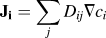
Introducing explicitly in the last term of Eq. (4), the divergence of fluxes
 ${{\bf{J}}_{\bf{i}}} = \sum\limits_j {{D_{ij}}\nabla {c_i}}$
, Eq. (9), can describe the evolution of interstitial and vacancy fields in a large system with appropriate boundary conditions. Equation (9) can be considered as the archetype of reaction-diffusion equations. Performing a linear stability analysis in the neighborhood of uniform steady state U
0 in the Fourier space, the evolution of the perturbation is dictated by the secular equation det(L
ij
− ωδ
ij
) = 0, where
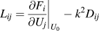 ${L_{ij}} = {\left. {{{\partial {F_i}} \over {\partial {U_j}}}} \right|_{{U_0}}} - {k^2}{D_{ij}}$
. Since the set of eigenvalues is discrete, simple instabilities correspond to a small number of situations
Reference Ghoniem and Walgraef9
:
-
(i) L ij has a vanishing eigenvalue at k = 0 and for μ = μc, we expect a transition between different homogeneous states with a critical point at μc.
-
(ii) L ij has a vanishing eigenvalue at |k| = k 0 and for μ = μc, the bifurcation induces a pattern-forming instability leading to spatially periodic structures.
-
(iii) L ij has two complex conjugate eigenvalues [(L) is a real] with vanishing real part for k = 0 and μ = μc, an Andronov–Hopf bifurcation appears leading to temporal oscillations of the limit cycle type.
-
(iv) L ij has two complex conjugate eigenvalues [(L) is a real] with vanishing real part for |k| = k 0 and μ = μc, traveling waves with well-defined spatiotemporal periodicity is produced.
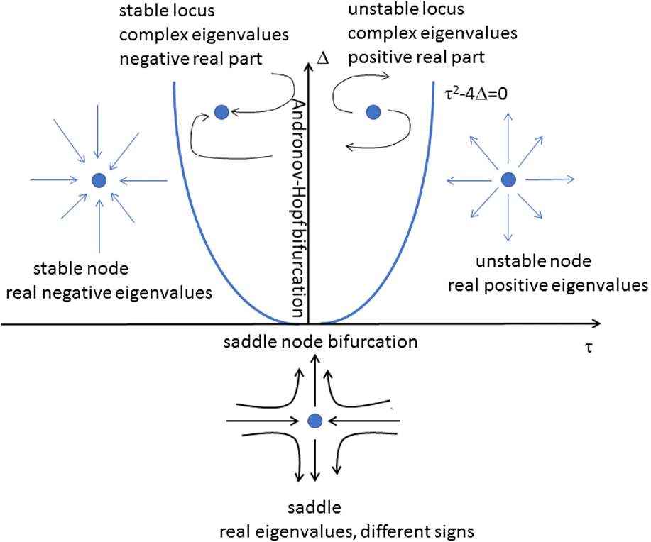
In 2D, the amplification rate satisfies ω2 − τω + Δ = 0, where τ and Δ are the trace and the determinant of the L matrix. Depending on the different values of τ and Δ, the evolution of the systems toward different attractors can be easily predicted (Fig. 5). For τ2 − 4Δ ≥ 0, one eigenvalue ω is positive and the steady state solution is unstable. The attractor reduces to a saddle point. The line τ2 − 4Δ = 0 is associated with a marginal stability. For τ ≤ 0, Δ ≥ 0, and τ2 − 4Δ ≥ 0, eigenvalues are all negative. The attractor is a stable node and uniform steady states are stable with respect to any small perturbations. For τ ≥ 0, Δ ≥ 0, and τ2 − 4Δ ≥ 0, all eigenvalues are positive leading to an unstable node; all steady states are unstable. For Δ ≥ 0 and τ2 − 4Δ ≤ 0, eigenvalues are complex conjugated and the steady state exhibits oscillations. For τ = 0, real parts of eigenvalues are positive and perturbation amplifies in time. The attractor is an unstable focus. For τ = 0, the real part of the eigenvalues is negative and the attractor is a stable focus. For τ = 0, the real part of ω is null and the attractor is a limit cycle. Figure 5 summarizes all possible fixed points in reaction diffusion problems.
Description of all possible fixed points in a 2D reaction diffusion problem.

The explicit introduction of gradient terms in the real space implies that possible space modulations (Turing patterns) of defect concentrations can appear in these reaction diffusion processes. From the knowledge of ω(k, μ) in the Fourier space, it is possible to determine the patterns’ modulation as well as the amplitudes of the modulation of the fields. To exemplify such a method, the evolution of dislocation loops under irradiation is analyzed hereinafter. The evolution of the dislocation loop density ρL (length per unit volume) is dictated by the three following coupled equations Reference Maydet and Russel27 :
 $${{{\rm{d}}{C_{\rm{i}}}} \over {{\rm{d}}t}} = {K_{\rm{i}}} - {K_{{\rm{iv}}}}{C_{\rm{i}}}{C_{\rm{v}}} + {D_{\rm{i}}}{\nabla ^2}{c_{\rm{i}}} - {D_{\rm{i}}}{c_{\rm{i}}}{Z_{\rm{i}}}\left( {{\rho _{\rm{n}}} + {\rho _{\rm{l}}}} \right)\quad,$$
 $${{{\rm{d}}{C_{\rm{v}}}} \over {{\rm{d}}t}} = \varepsilon {K_{\rm{i}}} - {K_{{\rm{iv}}}}{C_{\rm{i}}}{C_{\rm{v}}} + {D_{\rm{v}}}{\nabla ^2}{c_{\rm{i}}} - {D_{\rm{v}}}{Z_{\rm{v}}}\left( {{\rho _{\rm{n}}}\left( {{c_{\rm{v}}} - c_{\rm{v}}^{{\rm{eq}}}} \right) + {\rho _{\rm{L}}}\left( {{c_{\rm{v}}} - c_{\rm{v}}^{{\rm{eq}}}} \right)} \right)\quad,$$
 $${{{\rm{d}}{\rho _{\rm{L}}}} \over {{\rm{d}}t}} = {1 \over {\left| b \right|{r_0}}}\left( {\varepsilon {K_{\rm{i}}} - {\rho _{\rm{L}}}\left[ {{D_{\rm{i}}}{Z_{\rm{i}}}{c_{\rm{i}}} - D{E_{\rm{v}}}{Z_{\rm{v}}}\left( {{c_{\rm{v}}} - c_{\rm{v}}^{{\rm{eq}}}} \right)} \right]} \right)\quad,$$
where Z
i and Z
v are the capture efficiency of dislocation for interstitials and vacancies,
 $c_{\rm{v}}^{{\rm{eq}}}$
is the equilibrium concentration of interstitials close to the loop, and ε is the fraction of vacancies that collapse in the core of a displacement cascade producing a loop of radius r
0 associated with a Burgers vector b. ρN and ρL are the neutral and loop dislocation densities.
Reference Maydet and Russel27
In this approximation, long range elastic field induced by dislocations are neglected and the radius of dislocation is assumed to be constant. Density dislocation loops result from a balance between interstitial and vacancy concentration fields. Assuming that the evolution of the microstructure defined by ρL(x, t) is slower than the point defect field (an adiabatic-like approximation), the evolution of the vacancy loop density is dictated by
 $${{{\rm{d}}{\rho _{\rm{L}}}} \over {{\rm{d}}t}} = \left( {\varepsilon - \lambda {{\left( {k_{\rm{0}}^2 + {\nabla ^2}} \right)}^2}} \right){\rho _{\rm{L}}} + A{\left( {{\rho _{\rm{L}}}} \right)^2} - B{\left( {{\rho _{\rm{L}}}} \right)^3}\quad,$$
where ε, λ > 0, A, and B are phenomenological coefficients. Reference Maydet and Russel27
Equation (11) is the Haken
Reference Cross and Hohenberg31
equation extensively used to discuss nonequilibrium patterns. The amplification rate
 $\omega \left( k \right) = \varepsilon - \lambda {\left( {k_{\rm{0}}^2 - {k^2}} \right)^2}$
, associated with the linear part of the kinetic equations, exhibits a maximum at k
0 ensuring that spatial modulations of wave length
 $\lambda = {{2\pi } \over {{k_0}}}$
of ρL(x, t) take place in the system. An instability then occurs at ε = 0 for a spatial modulation of wave vectors of modulus k
0. For ε < 0, only the uniform steady state exists. For ε > 0, a one dimensional modulation stable steady state appears (rolls or stripes in 2D system and plane walls in 3D systems). This change at εc = 0 from an uniform solution to a modulated structure corresponds to a supercritical bifurcation plotted in Fig. 4(a). In the domain defined by k
− < k < k
+, ω(k) becomes positive and instabilities can propagate in the material. If ω(k, μ) depends only on the modulus of k, the system is said isotropic. If such a condition is not fulfilled, the system is said anisotropic.
A. Instabilities: hard and soft modes
Instabilities are associated with the maximum of the real part of the amplification rate
 ${{{\rm{d}}{\mathop{\rm Re}\nolimits} \left[ {\omega \left( {k,\mu } \right)} \right]} \over {{\rm{d}}k}}$
. This maximum is reached for a critical value of the wave vector k
c. Depending on values of Im[ω(k
c
, μ
c
)], different instability modes can propagate. For k
c = 0, soft modes propagate by analogy with the theory of phase transition. For non-null k
c values, hard modes propagate and the different directions of the propagation are given by all k
c nonequivalents to the space group associated with the invariant of the initial kinetic equation. The set of such critical wave vector is named the star of k
c.
Reference Tolédano and Dmitriev7
Steady states can then be defined by different values of Im[ω(k
c
, μ
c
)]:
-
(i) The critical wave vector associated with the maximum of the real part of the amplification rate can be null and Im[ω(k c , μ c )] = 0. A stationary state is produced and mainly dominated by long wave instabilities. No pattern is created.
-
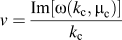
(ii) The critical wave vector associated with the maximum of the real part of the amplification rate can be null and Im[ω(k c , μ c )] is non-null. A periodic temporal state without spatial patterning is produced (limit cycle). For non-null values of Im[ω(k c , μ c )], the propagation front of the instability is thus defined by
 $v = {{{\mathop{\rm Im}\nolimits} \left[ {\omega \left( {{k_{\rm{c}}},{\mu _{\rm{c}}}} \right)} \right]} \over {{k_{\rm{c}}}}}$
.
-
(iii) For non-null k c values and Im[ω(k c , μ c )] = 0, a stationary spatial pattern is created.
-
(iv) For non-null k c and Im[ω(k c , μ c )] = 0 values, a double spatial and temporal pattern can be created.
The interplay between reaction diffusion processes is sufficient to explain spatial patterns and was first studied by Turing. Patterns produced do not depend on the detail of the kinetics under investigation but rather on the general mathematical expression for the kinetic equations. In this sense, these patterns exhibit a class of universality. As an example of radiation-induced Turing’s patterns, Fig. 6 displays the formation of a BCC void superlattice in Mo induced by 2-MeV N ions (at 1143 K and 100 dPa). Reference Sikka and Moteff32 Similar patterns have been observed in ceramic materials irradiated by He ions. Reference Beauford, Vallet, Nicolai and Bardot33
Electron micrograph displaying an ordered array of voids in W irradiated at 823 K in a fast neutron reactor at a fluence of 1022 cm−2. Reprinted with permission from Ref. Reference Sikka and Moteff32, Copyright 4218680185280, AIP Publishing LLC.

The linear analysis cannot by itself determine what type of microstructure is selected beyond the instability, i.e., for values of μ far from the critical control parameter value μc. Pattern selection is effectively determined by nonlinear terms. Reference Walgraef34 Fortunately, close to the instability threshold, space-time separation takes place between stable and unstable nodes. Stable modes can thus be adiabatically suppressed and the dynamics reduces to the nonlinear unstable mode dynamics. Only these modes govern the long time evolution of the system and capture asymptotic properties of the complete kinetic model in the vicinity of its bifurcation point. Performing such an adiabatic elimination, the stability of steady states of the system is dictated by amplitude equations.
B. Amplitude equation
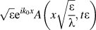
A k range exists for which all infinitesimal perturbations can grow in the vicinity of ε = 0 and ρL(x, t) can be written as
 $\sqrt \varepsilon {{\rm{e}}^{i{k_0}x}}A\left( {x\sqrt {{\varepsilon \over \lambda }},t\varepsilon } \right)$
, where A is an unknown function. From this analysis, new space scale and time scale emerge associated with
 $X = {x \over {\sqrt {{\varepsilon \over \lambda }} }}$
and
 $T = {t \over \varepsilon }$
.
For example, in the vicinity of εc = 0 (more generally in the neighborhood of the μc), ρL(x, t) exhibits a patterning of wave length
 $\lambda = {{2\pi } \over {{k_0}}}$
and its amplitude A(X, T) varies very slowly and satisfies simpler equations known as amplitude equations. Performing a scaling with the new variable X, T, the evolution of A(X, T) casts as
Reference Cross and Hohenberg31
 $${{{\rm{d}}A} \over {{\rm{d}}T}} = \left( {\varepsilon + 4k_0^2{{\left( {{\nabla _X}} \right)}^2}} \right)A - 3{\left| A \right|^2}A\quad .$$
This amplitude equation has the structure of a Landau–Ginzburg equation (due to the |A|2 term) analyzed in detail in the literature. Reference Cross and Hohenberg31 As a result, Eq. (12) describing spatial inhomogeneities of loop distribution (or void densities) has the generic structure. It is known to produce stripes and hexagonal structures in 2D systems and BCC lattices or planar wall structures in 3D systems (see Fig. 6). Hexagonal and BCC structures appear via subcritical bifurcation while stripes and walls appear via a supercritical bifurcation. Reference Ghoniem and Walgraef9 An expected sequence of selected patterns should develop increasing the irradiation flux from BCC as displayed in Fig. 6 to arrays of dislocations Reference Ghoniem and Walgraef9 as displayed in Fig. 1.
Steady states given by a modulated wave of wave length
 ${{2\pi } \over {{k_0}}}$
and amplitude
 ${A_k} = {\left( {\varepsilon - 4k_0^2{k^2}} \right)^{{1 \over 2}}}{{\rm{e}}^{i\psi }}$
, where ψ is an arbitrary phase for ε > 0. The bifurcation from a uniform to a modulated structure generates a band structure made of one pair of opposite wave vectors (k, −k) of modulus k
0. The final structure thus results from the growth of an arbitrary number of wave–vector pairs of arbitrary orientations leading to stripes with different orientations.
C. Eckhaus and zigzag instabilities
As the patterns under consideration spontaneously break the continuous invariant, different microstructures (Goldstone modes) characterized by their phase ψ(X, t) are expected to exist. These solutions exist in a domain of the parameter space limited by the marginal stability curve defined by
 $\omega \left( k \right) = \varepsilon - 4k_0^2{k^2} = 0$
. For a 2D pattern, the stability of different modulated phases is dictated by the evolution of a perturbation f(X, T)e
i(kx+ψ(X,T)) according to
 $${{\partial \psi \left( {X,Y,T} \right)} \over {\partial T}} = \left( {{D_X}{{{\partial ^2}} \over {\partial {X^2}}} + {D_Y}{{{\partial ^2}} \over {\partial {X^2}}}} \right)\psi \left( {X,Y,T} \right)\quad,$$
 $$f\left( {X,Y,T} \right) = - {{3k} \over {{{\left( {\varepsilon - 4k_0^2{k^2}} \right)}^{{1 \over 2}}}}}{{\partial \psi \left( {X,Y,T} \right)} \over {\partial X}}\quad,$$
where D X and D Y are the function of k 0 and ε.
The amplitude perturbation f(X, Y, T) exhibits a relaxation and the phase ψ(X, Y, T) follows a diffusive process occurring over a larger time scale. Reference Pomeau and Manneville35 Far from the bifurcation point ε = 0, the stability of patterns can thus be easily studied using this linear diffusive equation:
-
(i) D x > 0 and D y > 0 imply that the structure is stable. A perturbation relaxes via a diffusive process.
-
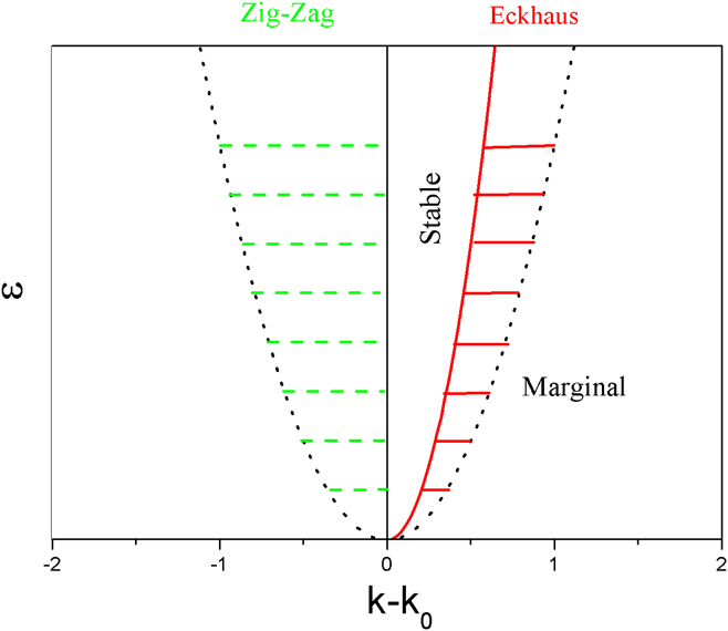
(ii) D x < 0, stripes relax to a stable structure via compression or dilatation parallel to walls or rolls according to the exact nature of the system. This instability is known as the Eckhaus instability.
-
(iii) D y < 0, the structure relaxes via modulations perpendicular to the structure stripes. This instability is named zigzag instability.
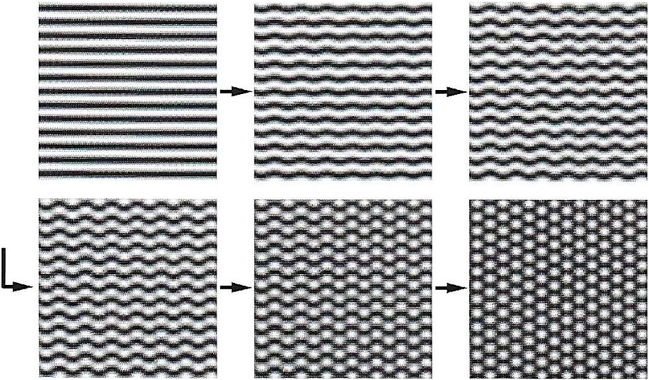
This stability analysis of the phase equation points out that transitions between an unstable “stripes” steady state to a stable hexagonal lattice Reference Ghoniem and Walgraef9 can be induced by a set of unstable modes lying in portions of the k − ε plane (Fig. 7). As an example, Fig. 8 highlights this transition in 2D simulations.
Stability diagram of stripe structures (2D) resulting from Eq. (11). The structure is unstable with respect to infinitesimal perturbation below the marginal curve (full line). Above the marginal curve (dotted line), Eckhaus (full hatched domain associated with negative D x values) and zigzag (dashed domain associated with negative D y values) perturbations can develop destabilizing the pattern. A stable domain insensitive to any perturbation exists leading to roll patterns.

To illustrate the effects of instabilities on pattern formation, the transition from an unstable stripe steady state to a stable hexagonal lattice via the propagation of Eckhaus (first row) and zigzag instabilities (second row) is displayed from SH simulations. Reprinted with permission from Instabilities and self-organization in materials Volume I: Fundamentals of nanoscience by Ghoniem (2008) Figs. 9.12 by permission of Oxford University Press.

Such an analysis can be straightforwardly applied to more complex structures like honeycomb lattices for which wave vectors k
j
of module k
0 defining the structure satisfy some geometric relations (k
1 + k
2 + k
3 = 0 leading to 2D honeycomb or 3D BCC structures). These structures resulting from the propagation of unstable critical modes defined by different k
j
do not follow the geometrical constraints. Patterns with modulations separated by angles slightly different from
 ${\pi \over 3}$
can appear for some positive values of ε and k values. The final structure is no more made by hexagons but is similar to rhombuses.
D. Topological defects
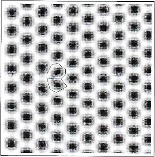
This part is largely inspired from the work of Walgraef. Reference Walgraef34 Although each individual spatiotemporal pattern resulting from the propagation of nonstable modes break transitional and rotational symmetries, different patterns grow in different parts of the system implying the formation of various defects connecting these different steady states. The existence of such structures generalizes the notion of topological defects defined for equilibrium structures and is generally the rule beyond pattern forming instabilities as it is the case in equilibrium phase transitions. As an illustration, Fig. 9 displays a penta–hepta pair of cells associated with a dislocation in hexagonal patterns. Reference Ghoniem and Walgraef9
Coarsening of hexagonal patterns in different directions leads to the formation of penta–hepta pairs of cells (black lines) in a hexagonal pattern. This topological defect can be understood as a dislocation. Reprinted from Instabilities and self-organization in materials Volume I: Fundamentals of nanoscience by Ghoniem (2008) Figs. 9.15 by permission of Oxford University Press.

This example points out that topological defects (antiphase boundary, disinclination, dislocation…) appear in pattern-forming systems. To clarify this point, reaction-diffusion dynamics is considered:
 $${{\delta U} \over {\delta t}} = f\left( {U,\mu } \right) + \alpha D\left( {U,\nabla } \right)\quad .$$
In the limit α → 0, the system reduces to a set of discrete equations where each point of the field U(x, t) evolves independently of its neighbors. Complex dynamics of the system may converge to different attractors such as in the case of Andronov–Hopf bifurcation for example. The basic idea Reference Coullet, Emilsson and Plaza36 is that the domains of attraction of disjoint attracting set do not intersect. Considering a system with two attracting sets, one part of the system lies in the domain of attraction of one set while another part lies in the second domain. The evolution of the system leads to the formation of a singularity (for α = 0) lying on a nonattractive set and forms the core of defects. The dimension of the defect core is the dimension of the embedded space d minus the number of unstable directions of the nonattracting set labeled n u, which can be understood as the co-dimension of the topological defect. This analysis tells us that co-dimension 1 defects correspond to points in 1D, to lines in 2D, and to planes in 3D while co-dimension 2 defect corresponds to points in 2D and filaments in 3D. When diffusion is turn on (non-null α values), the topological defects depend specifically on the system under consideration. If the domains of attraction of two different sets are identical, the diffusion effect is to smooth out the singularities. A typical example of this effect is the basic kink defect. For a stable limit cycle induced by an Andronov–Hopf bifurcation, n u = 2 and the formation of radial equiphases are created in 2D. The effect of diffusion is to regularize the equiphase forming a regular vortex observed in the XY model of ferromagnets or superfluids. Reference Walgraef34 Obvious generalizations of these vortexes in irradiated materials are the dislocations of layered or hexagonal patterns.
The key point of this analysis is that both a formation energy
 $\left( {F_i^d} \right)$
and a topological charge (m
i
) can be computed for each type of defects. Since this energy is nonnegligible, the probability for the nucleation of isolated defects in large systems is vanishingly small. However, a finite density of defects (dislocations pairs or dislocation clusters) of zero topological charges
 $\left( {\sum {{m_i} = 0} } \right)$
could nucleate in the structure leading to perfect array of defects explaining the formation of patterns as displayed in Figs. 1 and 2.
IV. PHASE FIELD APPROACH
Even if continuum models like the RT are sufficient to explain observed patterns created under irradiation, accretion and loss rate terms remain input parameters and must derive from more fundamental approaches. In the PF approach, these terms are directly derived from minimization of a “free energy” term. Reference Li, Hu and Stan2 In this sense, the PF method is self-consistent.
The PF method is an extension of the Landau theory of phase transition.
Reference Le Bellac, Mortessagne and Batrouni37
In his seminal work, Landau pointed out that phase transitions are associated with symmetry breaking and he defines the notion of OP, null in the high symmetric phase.
Reference Tolédano and Dmitriev7
For instance in paramagnetic to ferromagnetic transition, the rotational symmetry of the magnetization vector (the OP) is broken in the ferromagnetic phase leading to domains of well-defined orientation. To go a step beyond this approach, he intuited that the free energy of the system (more generally the thermodynamic potentials) is only a function of the OP related with LRO in materials. The main drawback of the Landau’s theory is to neglect the fluctuation (the evolution of the short-range order). In this sense, the PF approach is a mean-field approximation. To introduce spatial variation of the OP, η(x), extra (Ginzburg) terms ∇
p
(η(x)) were introduced in the free energy expression to take into account local inhomogeneities of the OP.
Reference Elder, Katakowski, Haataja and Grant8
Contrary to the RT described above, all information on the microstructure is only dictated by the variation of the free energy (more precisely its first variation
 ${{\delta F} \over {\delta \eta \left( {x,t} \right)}}$
) term without any need to external inputs.
A. Gradient and nongradient dynamics
Assuming that the evolution of a system can be modeled within the PF framework, the time variation of the LRO η(x, t) is assumed to be linked to the variation of an effective real free energy functional,
 $$\eqalign{ {{{\rm{d}}\eta \left( {x,t} \right)} \over {{\rm{d}}t}} = F\left( {\eta \left( {x,t} \right),\mu } \right) \cr = {F_{\rm{R}}}\left( {\eta \left( {x,t} \right),\mu } \right) + {F_{{\rm{NR}}}}\left( {\eta \left( {x,t} \right),\mu } \right)\quad . \cr}$$
Here, F was separated in two distinct terms. The first one F
R(η(x, t), μ) is associated with the relaxation part
 $- \Gamma {{\delta {\cal L}\left[ \eta \right]} \over {\delta \eta \left( {x,t} \right)}}$
of the dynamics (Γ being a positive operator). F
NR(η(x, t), μ) describes all nonrelaxing processes associated with the dynamics and is orthogonal to F
R(η(x, t), μ) for the given inner product.
Reference Ghoniem and Walgraef9
Different cases exist:
-
(i) If F NR = 0 and Γ is constant, the evolution of the system follows the line of steepest descent of
${\cal L}$
. The system is named a relaxation gradient flow. -
(ii) If F NR = 0 and Γ is not constant (system with conservation laws), transient patterns do not correspond to the lines of steepest descent of
${\cal L}$
. The system is a relaxation nongradient flow. -
(iii) If F NR is non-null, the status of the dynamics is still under investigation. The system is a nonrelaxation potential flow.


For systems described by relaxation flows, their behavior should be similar to those at equilibrium since a Lyapounov functional
 ${\cal L}\left[ \eta \right]$
can be determined. This functional plays the same role than the free energy and then can be understood as an “effective” free energy for dynamical systems. In particular, spatiotemporal patterns resulting from the minimization of
 ${\cal L}\left[ \eta \right]$
should appear and generate Turing-like patterns leading to the formation of topological defects. The next section is devoted to highlight this point discussing the nonequilibrium behavior of radiation-induced decomposition in nonmiscible alloys.
B. Application of the PF method: spinodal decomposition of alloys under irradiation
The spontaneous formation of patterns under irradiation was observed in many nonmiscible alloys for seventy years. The observed experimental patterns result from the existence of steady states. The main ingredient leading to steady states results from the competition between a thermally activated dynamics driving the system at temperature T to the equilibrium and an externally imposed particle exchange Γext(ϕ) regardless of the chemical identity of particles. This last dynamics is by essence athermal (T = ∞) and driven by the nature, the energy, and the flux ϕ of impinging particles. Martin
Reference Martin38
points out that the ordering induced under irradiation is indistinguishable from that of an equilibrium Ising model assuming that this exchange has an infinite range as expected.
Reference Bergersen and Racz39
The connection between these dynamical systems and equilibrium system is performed via the construction of a Lyapounov functional acting as an effective free energy. Thus, the dynamics of order–disorder transformation under irradiation for binary alloys with positive heat of mixing is indistinguishable to an equilibrium Cahn–Hilliard (CH) equation, the continuum counterpart of the Ising model, with infinite-range interactions. By analogy with the CH equation including elastic energy assumed to be of infinite range,
Reference Khatchaturyan6,Reference Huston, Cahn and Hilliard40
a “law of corresponding states” can be introduced for a system at temperature T via T
eff = T(1 + W). T
eff can be understood as the effective temperature of the system and
 $W = {{{\Gamma ^{{\rm{ext}}}}\left( \phi \right)} \over {\Gamma \left( {T,\phi } \right)}}$
(Γ(T, ϕ) is the thermally activated frequency of atoms promoting equilibrium) is a kinetic enhancement factor induced by the infinite range exchanges. From this analysis, T
eff becomes important at very low irradiation temperatures and do not affect the stability of precipitates at high temperature and low doses in agreement with experimental results.
Reference Adda, Beyeler and Brebec41
Since athermal exchanges are assumed to take place over an infinite range, such an approach is unable to describe patterns associated with spatial modulation of the chemical composition of the alloy at the mesoscopic scale, i.e., few tens of nanometers, experimentally observed under irradiation.
Reference Tsaur, Lau and Mayer42
To overcome this difficulty, the exchange of atoms occurring during the irradiation process is assumed to occur over a finite range with an average relocation distance R by analogy with phase separation induced by long range Coulomb interactions describing similar patterns.
Reference Chen and Khatchaturyan43
At equilibrium, the local composition (atomic fraction) given by the OP η(x, t) = c(x, t) − c
0, null in the disordered high temperature phase of uniform concentration c
0 in the
 ${A_{\bar{c}}}{B_{1 - \bar{c}}}$
alloy of average composition
 $\bar{c}$
is dictated by the CH equation routinely used to study the phase separation dynamics within the PF framework:
 $${{\partial \eta \left( {{\bf{x}},t} \right)} \over {\partial t}} = \Gamma \left( {T,\phi } \right){\nabla ^2}\left[ {{{\delta F\left[ \eta \right]} \over {\delta \eta \left( {{\bf{x}},t} \right)}}} \right]\quad,$$
where f(η(x, t)) is the free energy density which usually results from a Landau polynomial expansion
 $f\left( {\eta \left( {{\bf{x}},t} \right)} \right) = {{{a_2}} \over 2}\eta {\left( {{\bf{x}},t} \right)^2} + {{{a_3}} \over 3}\eta {\left( {{\bf{x}},t} \right)^3} + {{{a_4}} \over 4}\eta {\left( {{\bf{x}},t} \right)^4}$
, the parameters of which are fitted to satisfactorily reproduce the equilibrium phases.
Reference Demange, Luneville, Pontikis and Simeone44
In this equation, Γ(T, ϕ) is the averaged mobility of species assumed to be concentration independent.
Reference Bray45
On the other hand, the contribution of irradiation to the kinetic evolution of the alloy composition entering Eq. (16) can be expressed by the following equation Reference Sigmund and Gras-Marti22,Reference Simeone and Luneville23 :
 $$\eqalign{ {\left( {{{\partial \eta \left( {{\bf{x}},t} \right)} \over {\partial t}}} \right)^{{\rm{ext}}}} = {\Gamma ^{{\rm{ext}}}}\left( \phi \right)\left[ {\int {{p_{\rm{R}}}({\bf{x}} - {\bf{y}\right)}\eta \left( {{\bf{y}},t} \right){\rm{d}}{\bf{y}} - \eta } } \right] = {\Gamma ^{{\rm{ext}}}}\left( \phi \right)\left[ {{{\left\langle \eta \right\rangle }_{\rm{R}}} - \eta } \right]\quad, \cr}$$
where p R(x) ∝ exp(−|x|/R) is the density probability function describing the relocation of atoms set in motion by elastic collisions. R can be understood as a mean free path describing the relocation of atoms and is roughly equal to 1 nanometer. Reference Luneville, Mallick, Pontikis and Simeone46
By analogy with the studies of long range interactions at equilibrium, Reference Chen and Khatchaturyan43,Reference Ohta and Kawasaki47 the radiation-induced dynamics can be written as
 $${{{\partial \eta \left( {{\bf{x}},t} \right)} \over {\partial t}}^{{\rm{ext}}}} = {{{\Gamma ^{{\rm{ext}}}}\left( \phi \right)} \over 2}{\nabla ^2}{{\delta \left[ {\int {{\rm{d}}{\bf{x}}{\rm{d}}{\bf{y}}\eta \left( {{\bf{x}},t} \right)G\left( {{\bf{x}},{\bf{y}}} \right)\eta \left( {{\bf{y}},t} \right)} } \right]} \over {\delta \eta }}\quad,$$
where G(x, y) = G(|x − y|) expresses the spatial dependence of the radiation-induced relocation and can be understood as an effective long range interaction. This function G(x) is related with p
R(x) via ∇2
G(x) = p
R(x) − δ(x). The total dynamics resulting from the evolution in parallel to the thermal and the irradiation dynamics can thus result from the minimization of a Lyapounov functional
 ${\cal L}\left[ \eta \right] = F\left( {\eta \left( {x,t} \right)} \right) + {W \over 2}\left( {\int {{\rm{d}}x{\rm{d}}y\eta \left( {x,t} \right)G\left( {x,y} \right)\eta \left( {y,t} \right)} } \right)$
. This Lyapounov functional can be seen as an effective potential. Its minimization under the constraint of species conservation gives all possible steady states produced under irradiation. This effective free energy captures the physics associated with radiation damage in this particular system assessing the use of the PF method to handle the formation of the radiation-induced microstructure in nonmiscible alloys. The term W(ϕ, T) highlights the competition between relocation of atoms and their thermal diffusion.
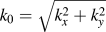
Figure 10 displays the 2D long-term evolution of η(x, t) resulting from a PF simulation. The power spectrum of the microstructure, i.e., the structure factor of η(x, t) resulting from the average of square of the Fourier transform of η(x, t) over initial configurations, exhibits a ring shape for long times revealing the existence of wave vector modulations of modulus k 0 assessing pattern formation.
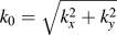
(a) 2D numerical simulation of the long-time microstructure (1000 in reduced units) of the AgCu alloy irradiated by 1 MeV Kr ions. Black (white) domains correspond to Cu rich (poor) regions. Boundary conditions imply that the calculated microstructure exhibits a point symmetry and two mirror symmetries. (b) Power spectrum of the microstructure. This power spectrum, i.e., the structure factor of the OP exhibits a Mexican hat shape. The maximum of its intensity exists for a well-defined modulus
 ${k_0} = \sqrt {k_x^2 + k_y^2}$
of wave vectors as displayed in figure (c).

A careful inspection of
 ${\cal L}\left[ \eta \right]$
clearly shown that order–disorder transitions (k
0 = 0) or a decomposition process occurs (non null k
0 values) for different (Wa, R) couples as shown in Fig. 11. From this analysis, it also becomes possible to compute the evolution of k
0 versus R for different W values as shown in Fig. 11. This evolution extracted from numerical PF simulation shows a clear linear evolution of k
0 with R
−1 in agreement with theoretical investigations resulting from the minimization of
 ${\cal L}\left[ \eta \right]$
.
Reference Simeone, Demange and Luneville48
This pattern formation is assessed by the peaked shape of the power spectrum (inset b in Fig. 10). The variation of k
0 with the parameters R and W points out a supercritical bifurcation of the dynamical system for the control parameter
 $\mu = \sqrt {W{R^4}} - 1$
(inset c in Fig. 10). Below μc = 0, relocation of atoms are not sufficient to counterbalance the thermal diffusion and the spinodal decomposition takes place under irradiation. For μc > 0, a balance between the two competitive dynamics occurs leading to the formation of modulated structures of wave vectors (k) of non-null modulus k
0 minimizing
 ${\cal L}\left[ \eta \right]$
.
(a) Evolution of k
0 versus R for different W values (black squares: W = 0.04, open circles: W = 0.7) and (b) k
0 values are extracted from the maximum of the universal structure factor obtained from simulations. (c) The evolution of k
0 versus the control parameter
 $\mu = \sqrt {W{R^4}} - 1$
displays a supercritical bifurcation.

Patterns produced under irradiation result from slow composition modulations in space and time of simple basic patterns defined by the wave vector of modulus k
0 minimizing
 ${\cal L}\left( t \right)$
. Although each individual stationary pattern breaks transitional and rotational symmetries (Fig. 12), different patterns grow in different parts of the system implying the formation of various defects connecting these different steady states
Reference Ghoniem and Walgraef9
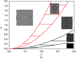
as displayed in Fig. 12. These patterns depend not only on R and W but also on the average composition of the nonmiscible alloys.
2D phase diagram for steady states obtained from
 ${\cal L}\left( t \right)$
in the one-mode approximation. Depending on the averaged composition
 $\bar{\psi }$
(in reduced units), stripes, bubbles in hexagonal networks and constant phase can be created. Hatched areas correspond to co-existence domains. This phase diagram is validated by numerical simulations (microstructure drawings). All simulations were performed for Δ = 0.2, R = 3, t = 3000 and the domain size equal to 200 in reduced units.

V. CONCLUSION
More than fifty years were devoted to show that irradiation of materials with energetic particles induces drastic changes in their microstructure and then induces important variation of their physicochemical properties (hardening, swelling…). The radiation response of materials is important in various technological fields ranging from nuclear industry to microelectronics and surface engineering. The existence of an extensive experimental database not only for metals and alloys Reference Dunlop, Rullier-Albenque, Jaouen, Templier and Davenas26 but also for ceramics Reference Simeone, Costantini, Luneville, Desgranges, Trocellier and Garcia12 allows us to present a large perspective on the physical nature of self organization in irradiated materials responsible for drastic modification of the microstructure under irradiation. The challenge in the prediction of these radiation-induced microstructures results from the integration of different mechanisms acting on different space and time scales in a unified framework. Even if the large amount of defects produced under irradiation drives the system far from equilibrium implying very complex and specific mechanisms, it seems that the final microstructure-like patterning do not depend on the specific mechanism under consideration and can be described within mean field approaches like the RT approximation. After describing in detail, mathematical approaches allowing us to discuss the long-term evolution of the patterns produced under irradiation (amplitude equations, Reference Cross and Hohenberg31 phase equations, Reference Pomeau and Manneville35 and Eckhaus instabilities Reference Cross and Hohenberg31 ), the interest of the PF method as a self-consistent mean-field approximation is presented. Neglecting specific details on the underlying physics, the PF approximation highlights the universal feature of radiation-induced patterns. The time-dependent classical density theory seems to point out at least formally the existence of a possible free energy functional (more general a thermodynamic potential) far from equilibrium assessing the use of the PF approach to discuss far from equilibrium situations. Reference Cross and Hohenberg31 However, this powerful method suffers from several limitations. As the PF method is a mean field approach, the free energy defining the system at equilibrium suffers from many limitations. This free energy is highly sensitive to the short-range order neglected in the PF approximation and its entropy does not take into account thermal vibrations which are usually in alloys and metals larger than the configuration entropy. To overcome this difficulty, the free energy is usually fitted on experimental phase diagram if they exist. Due to the large number of phenomenological parameters, this approach remains qualitative. However, multiscale approaches coupling MD Reference Demange, Luneville, Pontikis and Simeone44 and Monte Carlo Reference Opplestrup, Bulatov, Gilmer, Kalos and Sadigh49 simulations may overcome this difficulty leading to predictive methods. In radiation damage processes, three different time scales exist: the relaxation of point defects like interstitials and vacancies, the evolution of the short-range order terms, and the time variation of the LRO. In the PF approach, the time relaxation of point defects and short range order parameters is assumed to be very fast. Under such an “adiabatic” approximation, these variables are then fixed to their stationary values. This approximation remains difficult to assess. Moreover, the coarse graining process neglecting short-range order correlations in the PF approach does not allow a description of interfaces at the atomic scale and then leads difficult to reproduce the impact of these interfaces on mechanical properties of irradiated materials like elastic constants even if the elastic interaction between precipitates is naturally described in this framework. On the other hand, Langevin forces describing the possibility for the system to explore different minima of the Lyapounov functional depend on the coarse grained size avoiding fully quantitative predictions.
ACKNOWLEDGMENT
It is a pleasure to thank M. Athenes and A. Forestier for numerous stimulating discussions on dissipative systems and gradient flow systems.