1 Introduction
The migration of a fluid through a porous rock has received considerable interest over many decades (Dagan Reference Dagan1984; Hess, Wolf & Celia Reference Hess, Wolf and Celia1992; Berkowitz, Scher & Silliman Reference Berkowitz, Scher and Silliman2000; Paster, Bolster & Benson Reference Paster, Bolster and Benson2013). Such flows are of concern in many industrial and environmental applications including radioactive waste disposal, the flow of contaminants in freshwater aquifers, enhanced oil recovery and the sequestration of
 $\text{CO}_{2}$
within geological storage reservoirs (Lake Reference Lake1989; Phillips Reference Phillips2009; Woods Reference Woods2014). In order to learn about the nature of such flows in the ground, and obtain some constraints on the permeability of the host aquifer, it has been proposed to add passive tracers to the flow and analyse samples at observation wells (Bickle Reference Bickle2009; Mathieson et al.
Reference Mathieson, Midgely, Wright, Saoula and Ringrose2011; Kampman et al.
Reference Kampman, Bickle, Maskell, Chapman, Evans, Purser, Zhou, Schaller, Gattacceca, Bertier, Chen, Turchyn, Assayag, Rochelle, Ballentine and Busch2014). For example, in the
 $\text{CO}_{2}$
storage project at the Otway Basin, Australia, tracers were added to the injected gas to measure and verify the breakthrough of
 $\text{CO}_{2}$
at a production well (Stalker et al.
Reference Stalker, Boreham, Underschultz, Freifeld, Perkins, Schacht and Sharma2015). It is also possible to use naturally occurring isotopes to monitor the sequestration of
 $\text{CO}_{2}$
(Györe et al.
Reference Györe, Stuart, Gilfillan and Waldron2015).
Much of the previous work on tracer migration has focused on the effect of heterogeneity on the dispersion in a pressure-driven flow (Dagan Reference Dagan1984; Eames & Bush Reference Eames and Bush1999; Phillips Reference Phillips2009). However, Farcas & Woods (Reference Farcas and Woods2016) showed that longitudinal dispersion is possible in flow in a layered porous medium, even if the layers have constant permeability. Porous rocks often have low permeability baffles which act as a barrier to the vertical migration of a buoyant fluid such as
 $\text{CO}_{2}$
. Hesse & Woods (Reference Hesse and Woods2010) illustrated how the lateral spreading beneath these baffles can lead to longitudinal dispersion. Such advection-driven dispersion is controlled by the geometry and length scale of the formation, which can lead to much more rapid dispersive spreading of the flow compared to the effects of pore-scale dispersion or molecular diffusion. In this paper, we focus on the regime in which shear-driven dispersion of a tracer dominates, and so we neglect the effects of smaller-scale mixing processes, which may however become important at later times as shown in the appendix A.
We consider the migration of a tracer within a permeable layer in which the permeability varies linearly with height. It has previously been shown that contrasts in permeability lead to shear in the flow profile (Bjorlykke Reference Bjorlykke1993; Woods & Mingotti Reference Woods and Mingotti2016). In the absence of diffusion, the migration of a tracer is controlled by the shear and the interaction with the nose of the current. The shape of the nose of a current supplied by a constant flux migrating through a finite depth aquifer in which the permeability varies linearly with depth was studied by Hinton & Woods (Reference Hinton and Woods2018). They found four regimes for the late-time evolution of the flow. These depend on the viscosity ratio and the variation of permeability with depth. The regimes include a rarefaction wave which spreads at a rate proportional to time,
 $t$
, a shock-like front of fixed length, a mixture of shock-like regions and growing rarefaction regions, and an interface which spreads laterally at a rate proportional to
 $t^{1/2}$
. In each case, the flow is primarily driven by the pressure owing to injection and the role of buoyancy is secondary. In this paper, we explore the migration of a tracer in each of these regimes.
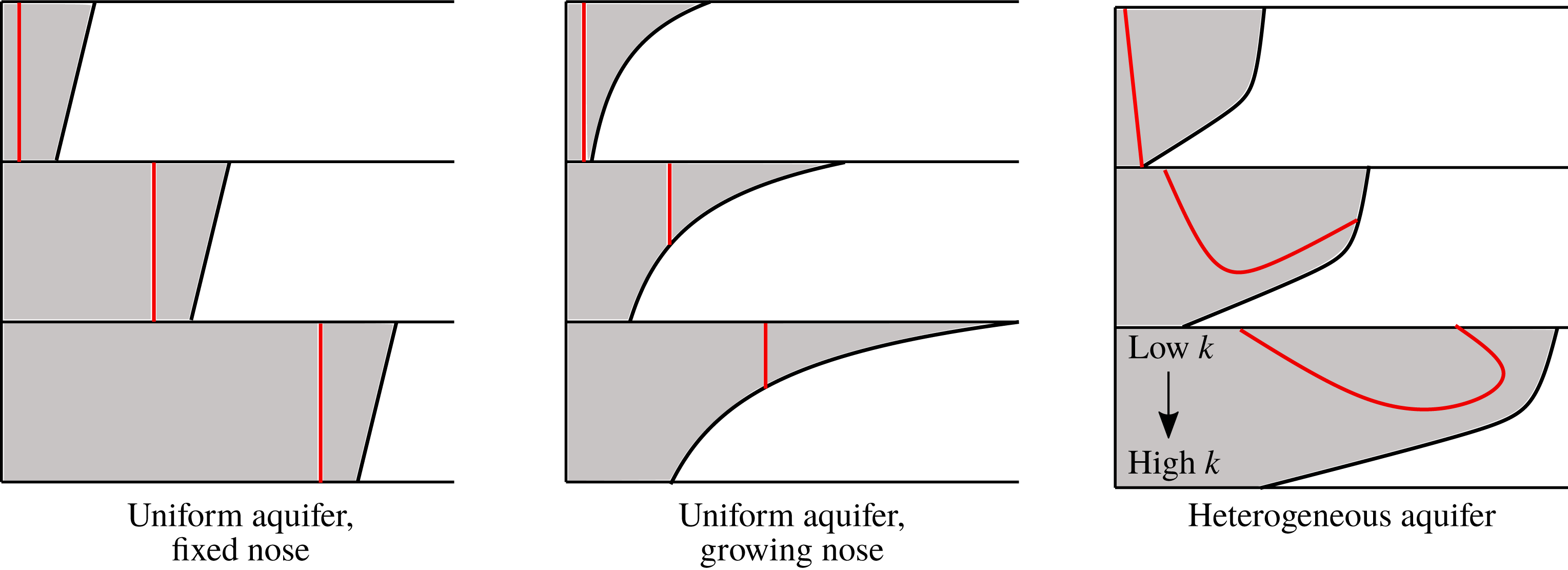
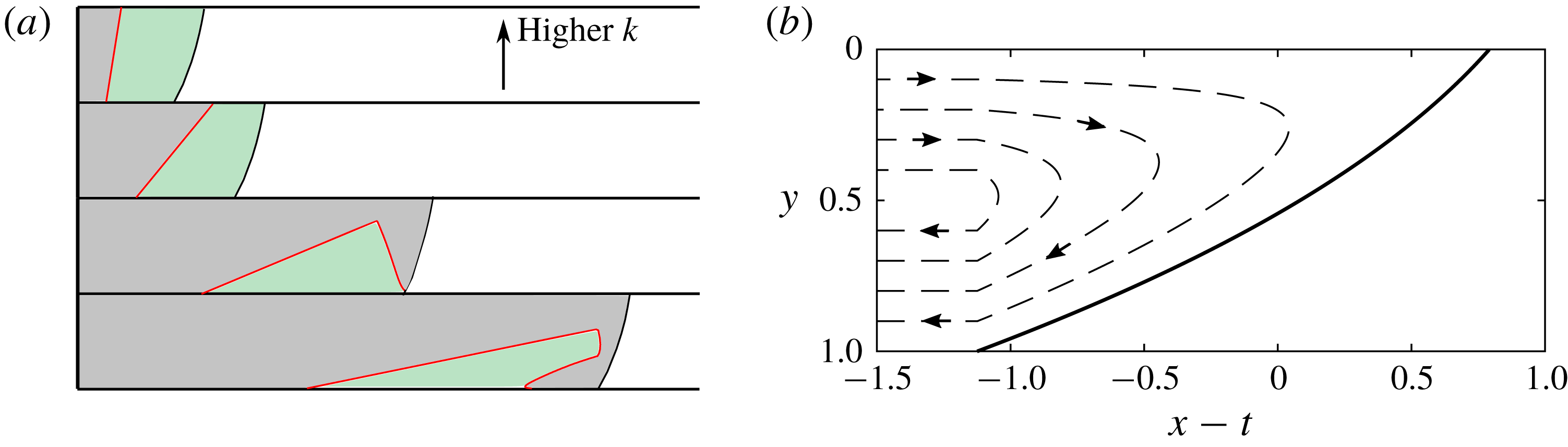
However, before launching into this analysis, it is useful for reference to describe the motion of a tracer within the flow in a uniform aquifer distinguishing between the cases in which the nose is of fixed shape and volume and in which the nose gradually spreads with time. Since the flow is uniform across the depth of the aquifer, there is no dispersion associated with the flow, but the location of the tracer relative to the front of the flow does change depending on whether the volume of the fluid in the nose of the current grows in time or remains fixed. In the case that the nose forms a fixed travelling-wave structure, the tracer remains a fixed distance behind the nose (see figure 1 a). If instead the nose region grows, the tracer is advected into continually shallower regions of the nose (see figure 1 b).
Schematic diagram showing the interaction between injected tracer (red pulse) and the nose region of the current. For a uniform aquifer in which the nose is fixed, the tracer remains a constant distance behind the interface. When the nose is growing, the tracer is carried into the nose. In a heterogeneous aquifer, tracers undergo a shear and the tracers in the fastest moving regions enter the nose.

In § 3, we review the four flow regimes which arise in an aquifer with a vertical gradient of permeability (Hinton & Woods Reference Hinton and Woods2018). The shear in these flows leads to dispersion of the tracer upstream of the nose and we examine how the dispersing tracer interacts with the nose region. In § 4, we investigate the first of the four flow regimes in which the nose of the flow continually grows (see figure 1 c). We show that the tracer may migrate towards the front of the nose as in the case of a uniform aquifer, or that the tracer may initially enter the nose, but then slow down relative to the speed of the nose, and may in fact subsequently advance more slowly than the trailing edge of the nose.
In § 5, we explore the interaction of the shearing of the tracer with a nose of fixed shape. Now the nose is a travelling wave which moves at the mean flow speed owing to mass conservation. The cross-channel shear associated with the variation of the permeability leads to a range of heights at which the flow is faster than the mean speed. The combination of these two effects means the tracer can catch and enter the fixed nose. However, mass conservation requires that the tracer which enters the nose subsequently leaves the nose and this occurs through the migration of the tracer into lower permeability regions where it is then left behind as the nose continues to advance. In § 6, we explore the dispersion which arises in the more complex case in which the interface consists of a growing rarefaction region and a vertical shock region. The fourth regime, in which the interface grows in proportion to
 $t^{1/2}$
, occurs only in a uniform aquifer and hence we cannot consider the influence of a shear flow in this case.
Finally, in § 7, we summarise our results and briefly discuss some implications for
 $\text{CO}_{2}$
sequestration.
2 Vertically uniform aquifer
In this section we consider the migration of tracer in a vertically uniform aquifer. There are three late-time regimes and we begin by finding the shape of the nose in each. We then introduce a tracer into the flow, and consider how it migrates in each regime. We show that the migration of the tracer is controlled by whether the nose is growing or has fixed volume. A vertical line of tracer added to the injectate at
 $X=0$
will remain vertical because there is no shear in the flow.
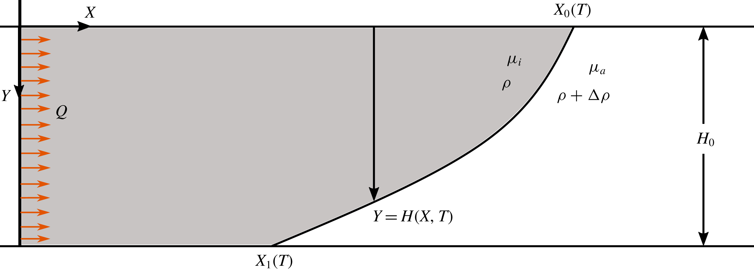
Cartoon of fluid injection into a confined aquifer. Fluid is injected from a line source at
 $X=0$
which releases a pulse of tracer at some late time.

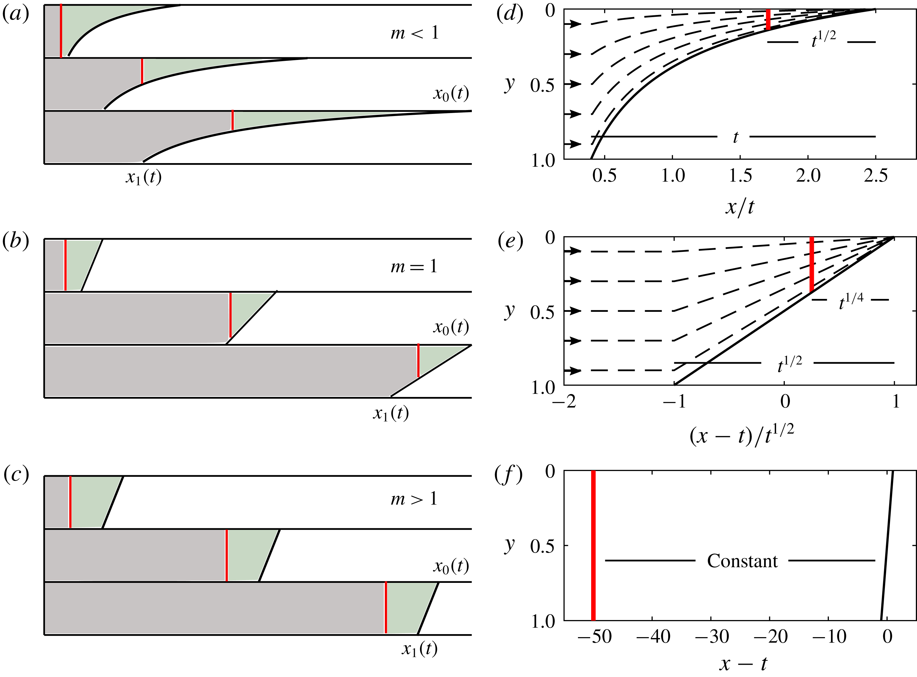
Tracer injection into a uniform porous medium. Panels (a–c) show cartoons of the position of tracer (red) relative to the nose at three times. The area of fluid ahead of the tracer (green region) is constant. Panels (d–f) show the position of the red tracer in coordinates moving with the nose region, and the particle paths (dashed lines). (a,d) The case of a less viscous injected fluid. The extent of the nose grows in proportion to
 $t$
and the distance between the tracer and the leading contact point in proportion to
 $t^{1/2}$
. (b,e) Equally viscous fluids. The nose grows in proportion to
 $t^{1/2}$
with the tracer a distance proportional to
 $t^{1/4}$
from the leading contact point. (c,f) More viscous injected fluid. The fixed shape nose and the tracer both travel at the mean flow speed and hence the distance between them is constant.

2.1 Review of the interface evolution in a uniform aquifer
If liquid of density
 $\unicode[STIX]{x1D70C}$
and viscosity
 $\unicode[STIX]{x1D707}_{i}$
is injected from a line source at
 $X=0$
with a flow rate
 $Q$
into a horizontal, laterally extensive aquifer initially filled with liquid of density
 $\unicode[STIX]{x1D70C}+\unicode[STIX]{x0394}\unicode[STIX]{x1D70C}$
and viscosity
 $\unicode[STIX]{x1D707}_{a}$
, and the aquifer has depth
 $H_{0}$
, porosity
 $\unicode[STIX]{x1D719}$
(figure 2), then the flow is controlled by the combination of the applied pressure associated with the injection and the buoyancy force. We can scale the depth, length and time using the following relations
 $$\begin{eqnarray}h=\frac{H}{H_{0}},\quad y=\frac{Y}{H_{0}},\quad x=\frac{Q}{UH_{0}^{2}}X,\quad t=\frac{Q^{2}}{\unicode[STIX]{x1D719}UH_{0}^{3}}T,\end{eqnarray}$$
where
 $$\begin{eqnarray}U=\frac{\unicode[STIX]{x0394}\unicode[STIX]{x1D70C}gK}{\unicode[STIX]{x1D707}_{i}}\end{eqnarray}$$
is the characteristic buoyancy velocity of the injectate, and
 $K$
is the constant permeability. In this paper, we use capital letters to denote dimensional quantities and lower case for dimensionless quantities, with the exception of the density, the viscosity and gravity,
 $g$
.
Once the injectate has spread far from the well and provided that the horizontal extent is much greater than the depth of the aquifer, the assumption that the cross-flow pressure gradient is hydrostatic (see Bear Reference Bear1971) leads to the dimensionless equation for the depth of the injected flow,
 $h(x,t)$
,
 $$\begin{eqnarray}\frac{\unicode[STIX]{x2202}h}{\unicode[STIX]{x2202}t}+\frac{\unicode[STIX]{x2202}}{\unicode[STIX]{x2202}x}\left(\frac{h}{m+(1-m)h}\right)=\frac{\unicode[STIX]{x2202}}{\unicode[STIX]{x2202}x}\left(\frac{mh(1-h)}{m+(1-m)h}\frac{\unicode[STIX]{x2202}h}{\unicode[STIX]{x2202}x}\right)\!,\end{eqnarray}$$
where we have assumed the two fluids are immiscible and there is a sharp interface between them. The viscosity ratio of the two fluids is (see figure 2)
 $$\begin{eqnarray}m=\frac{\unicode[STIX]{x1D707}_{i}}{\unicode[STIX]{x1D707}_{a}}.\end{eqnarray}$$
The second term on the left-hand side of (2.3) represents the advection associated with the applied pressure whilst the term on the right-hand side represents the diffusive slumping of the injected fluid owing to buoyancy. After an initial transient, the flow has a fully flooded region in which
 $h=1$
and a nose region in which
 $0<h<1$
. We use the term ‘trailing contact point’ to describe the point at which the interface touches the bottom boundary at the back of the nose region, denoted
 $X_{1}(T)$
in figure 2. The point at the front of the nose along the top boundary is the ‘leading contact point’ (
 $X_{0}(T)$
in figure 2). Note that in the dimensionless variables,
 $$\begin{eqnarray}h(x_{0}(t),t)=0,\quad \text{and}\quad h(x_{1}(t),t)=1.\end{eqnarray}$$
Three different late-time asymptotic regimes for the evolution of the nose can emerge depending on whether
 $m$
is less than, equal to or greater than
 $1$
(see Huppert & Woods Reference Huppert and Woods1995; Pegler, Huppert & Neufeld Reference Pegler, Huppert and Neufeld2014; Zheng et al.
Reference Zheng, Guo, Christov, Celia and Stone2015). With a less viscous injectate (
 $m<1$
), the extent of the nose region increases in proportion to
 $t$
and the term associated with the buoyancy on the right-hand side of (2.3) can be neglected. The late-time shape is then given by (Pegler et al.
Reference Pegler, Huppert and Neufeld2014)
 $$\begin{eqnarray}h(x,t)=\frac{\sqrt{{\displaystyle \frac{mt}{x}}}-m}{1-m},\end{eqnarray}$$
and the positions of the trailing (
 $h=1$
) and leading (
 $h=0$
) contact points are
 $x_{1}(t)=mt$
and
 $x_{0}(t)=t/m$
, respectively (see figure 3
a).
In the case of fluids with the same viscosity (
 $m=1$
), the term in the governing equation (2.3) associated with the buoyancy balances the term associated with the advection. The extent of the nose grows in proportion to
 $t^{1/2}$
and the depth is given by
 $$\begin{eqnarray}h={\textstyle \frac{1}{2}}(1-\unicode[STIX]{x1D709}),\quad \text{where}\;\unicode[STIX]{x1D709}=(x-t)/\sqrt{t},\quad \text{for}\;-1\leqslant \unicode[STIX]{x1D709}\leqslant 1,\end{eqnarray}$$
and the contact points are
 $$\begin{eqnarray}x_{1}(t)=t-t^{1/2},\quad x_{0}(t)=t+t^{1/2}\end{eqnarray}$$
(see figure 3
b). The depth in the nose region for the present case of
 $m=1$
(2.7) is a singular limit of the case
 $m<1$
. This is because the effects of buoyancy can no longer be neglected when
 $m=1$
.
With a more viscous injectate (
 $m>1$
), a steadily travelling shock moving with the speed of the mean flow develops across the entire depth of the aquifer. To model the shock it is convenient to transform to coordinates moving with the shock. We then find the constant shape of the nose is a straight line with gradient
 $(1-m)/m$
(see figure 3
c). The equation for the depth in the nose region is
 $$\begin{eqnarray}h(x,t)=\frac{1}{2}+\frac{1-m}{m}(x-t),\quad \text{for}\;x_{1}(t)<x<x_{0}(t),\end{eqnarray}$$
where the contact points are
 $$\begin{eqnarray}x_{0}(t)=t+\frac{m}{2(m-1)},\quad x_{1}(t)=t-\frac{m}{2(m-1)}.\end{eqnarray}$$
The late-time shape (2.9) is accurate after times of order (cf. Zheng et al. Reference Zheng, Guo, Christov, Celia and Stone2015)
 $$\begin{eqnarray}t_{s}=\frac{m}{1-m},\end{eqnarray}$$
which corresponds to the time taken to supply the volume of fluid in the fixed travelling nose.
In each regime, the dimensionless Darcy velocity in the current is
 $$\begin{eqnarray}u=\frac{1-m(1-h){\displaystyle \frac{\unicode[STIX]{x2202}h}{\unicode[STIX]{x2202}x}}}{m+(1-m)h}.\end{eqnarray}$$
The second term in the numerator arises from buoyancy forces, and the first is associated with the injection pressure. The incompressibility condition for the flow,
 $\unicode[STIX]{x1D735}\boldsymbol{\cdot }\boldsymbol{u}=0$
, can be used to calculate the vertical velocity from the horizontal velocity,
 $$\begin{eqnarray}v=-\int _{0}^{y}\frac{\unicode[STIX]{x2202}u}{\unicode[STIX]{x2202}x}\;\text{d}y,\end{eqnarray}$$
and
 $v(y=0)=0$
as there is no flux across the upper boundary. In dimensional terms, the ratio of the vertical velocity to the horizontal velocity is
 $$\begin{eqnarray}b=\frac{Q}{UH_{0}}.\end{eqnarray}$$
For the hydrostatic assumption to apply, we require the vertical velocity to be much smaller than the horizontal velocity. In an interface which grows,
 $v$
decays in time and this assumption is always valid at late times. However, for an interface of constant extent, we require that
 $b\ll 1$
.
2.2 Tracer injection
The injection of fluid begins at
 $t=0$
. We consider releasing a pulse of tracer across the entire depth of the aquifer at a dimensionless time
 $t_{R}$
after the first injection of fluid. We assume
 $t_{R}$
is sufficiently large that the interface between the two fluids has evolved to one of the late-time regimes. We assume the tracer does not react with the injectate or the rock, the interface is gravitationally stable and we assume there is no mixing across the interface. Tracer particles are advected by the flow field (diffusion is neglected, see appendix A for details).
2.3 Tracer migration for a less viscous injected fluid (
 $m<1$
)

At late times the interface is long and thin; the role of buoyancy is negligible. Behind the nose region, the along-channel velocity is 1 which is greater than
 $m$
, the velocity of the trailing contact point (see figure 3
a). Using these two velocities and the release time of tracer,
 $t=t_{R}$
, we calculate that the line of tracer enters the nose region at a time,
 $$\begin{eqnarray}t_{E}=\frac{t_{R}}{1-m}.\end{eqnarray}$$
The along-channel velocity in the nose region can be calculated from (2.12),
 $$\begin{eqnarray}u=\frac{1}{m+(1-m)h},\end{eqnarray}$$
where we have neglected the component of velocity owing to buoyancy, consistent with the assumption used in deriving the interface shape. Combining this with our expression for the depth,
 $h(x,t)$
(equation 2.6), and mass continuity (2.13), we derive the equations for the particle paths in the nose region,
 $$\begin{eqnarray}\frac{\text{d}x}{\text{d}t}=\left(\frac{x}{mt}\right)^{1/2}\!,\quad \frac{\text{d}y}{\text{d}t}=-\frac{y}{2(mxt)^{1/2}}.\end{eqnarray}$$
We can solve (2.17a ) for the horizontal position of a vertical line of tracer as it is advected in the nose,
 $$\begin{eqnarray}x(t;a_{0})=\left[\left(\frac{t}{m}\right)^{1/2}-a_{0}\right]^{2},\end{eqnarray}$$
where
 $a_{0}$
is a constant which can be found using the time,
 $t=t_{E}$
(2.15), at which the line of tracer passes the trailing contact point,
 $x_{1}(t)=mt$
, and enters the nose,
 $$\begin{eqnarray}a_{0}=\left(\frac{t_{E}}{m}\right)^{1/2}-(Mt_{E})^{1/2}.\end{eqnarray}$$
Relative to the leading contact point,
 $x_{0}(t)=t/m$
, the position is
 $$\begin{eqnarray}x_{L}=x_{0}(t)-x(t;a_{0})=2a_{0}\left(\frac{t}{m}\right)^{1/2}-a_{0}^{2}.\end{eqnarray}$$
At late times, at leading order, (2.20) implies that the distance between the line of tracer and the leading contact point grows in proportion to
 $b_{0}t^{1/2}$
where
 $$\begin{eqnarray}b_{0}=\frac{2a_{0}}{m^{1/2}}=2\frac{(1-m)^{1/2}}{m}t_{R}^{1/2}.\end{eqnarray}$$
The volume of fluid ahead of the tracer is constant (green region in figure 3
a) and hence the line of tracer travels into continually shallower regions of the growing nose. This can also be seen by comparing the distance to the leading contact point,
 $t^{1/2}$
, with the extent of the interface which grows in proportion to
 $t$
(see figure 3
a).
2.4 Tracer migration for equally viscous fluids (
$m=1$
)

It was shown in § 2.1 that the structure of the nose in the case of isoviscous fluids is singular owing to the balance between the term associated with buoyancy and the term associated with advection. The horizontal velocity upstream of the nose is 1 and hence a line of tracer released from
 $x=0$
at
 $t=t_{R}$
reaches the trailing contact point,
 $x_{1}(t)=t-t^{1/2}$
(2.8), and enters the nose at a time,
 $$\begin{eqnarray}t_{E}=t_{R}^{2}.\end{eqnarray}$$
The along-channel velocity in the nose is given by (2.12),
 $$\begin{eqnarray}u=1-(1-h)\frac{\unicode[STIX]{x2202}h}{\unicode[STIX]{x2202}x}.\end{eqnarray}$$
Combining this with our expression for the depth of the current,
 $h(x,t)$
(equation 2.7), and mass continuity (2.13), we derive the equations for the velocity and hence the particle paths in the nose region,
 $$\begin{eqnarray}\frac{\text{d}x}{\text{d}t}=1+\frac{x-(t-t^{1/2})}{4t},\quad \frac{\text{d}y}{\text{d}t}=\frac{-y}{4t}.\end{eqnarray}$$
Solving (2.24a ) for the horizontal position of the vertical line of tracer gives
 $$\begin{eqnarray}x=t+t^{1/2}-a_{1}t^{1/4},\end{eqnarray}$$
where
 $a_{1}$
is a constant which can be found using the time at which the line of tracer enters the nose,
 $$\begin{eqnarray}a_{1}=2t_{E}^{1/4}=2t_{R}^{1/2}.\end{eqnarray}$$
The distance between the line of tracer and the leading contact point,
 $x_{0}(t)=t+t^{1/2}$
, grows in proportion to
 $t^{1/4}$
. The distance from the trailing contact point grows in proportion to
 $t^{1/2}$
because the interface grows in proportion to
 $t^{1/2}$
(see figure 3
b). Using the vertical velocity (2.24b
), we calculate that the height of the line of tracer decays in proportion to
 $t^{-1/4}$
.
We found in § 2.1 that the shape of the nose region in the case
 $m=1$
is a singular limit of the shape for
 $m<1$
. Similarly, the migration of tracer described in the present section for
 $m=1$
is a singular limit of the migration described in § 2.3 for
 $m<1$
. The results in the case
 $m=1$
are analogous to those of § 2.3, with the exponents halved. For
 $m<1$
, the distance between the leading contact point and the tracer grows as
 $b_{0}t^{1/2}$
(2.20). The coefficient
 $b_{0}$
tends to
 $0$
as
 $m\rightarrow 1$
, and the analogous result for
 $m=1$
gives the distance growing in proportion to
 $t^{1/4}$
, a singular limit.
2.5 Tracer migration for a more viscous injected fluid (
$m>1$
)

When the injected fluid is more viscous than the ambient fluid, the nose takes the form of a fixed travelling wave, shown as a black line in figure 3(c). A line of tracer is released at
 $t=t_{R}$
from
 $x=0$
; it is initially behind the interface in the fully flooded region. The nose and the line of tracer both travel at the injection velocity, which in dimensionless terms is
 $1$
. The tracer remains a constant distance behind the nose (see figure 3
c). The nose of the current never influences the dynamics. In the limit as
 $m\rightarrow 1$
, the interface gradient (2.9) tends to
 $0$
and the nose becomes infinitely long and would influence the tracer; the case
 $m=1$
is a singular limit of the fixed nose regime.
2.6 Summary of tracer migration in a uniform aquifer
We have found that when fluid is injected into a uniform aquifer of finite depth and the viscosity of the injected fluid is less than or equal to the viscosity of the ambient fluid (
 $m\leqslant 1$
), the nose region grows in time, supplied by fluid from behind. There is no dispersion of the tracer but it is carried into continually shallower regions of the nose. When
 $m>1$
, the nose has fixed shape, and all the fluid moves at the same velocity, remaining a fixed distance behind the nose.
3 Model for flow in an aquifer with a vertical gradient of permeability
We now extend the analysis from § 2, for tracer migration in a uniform aquifer, to incorporate the influence of vertical heterogeneities. We first review the model of Hinton & Woods (Reference Hinton and Woods2018) which describes injection into a confined aquifer in which the dimensional permeability,
 $K(Y)$
, varies with the dimensional depth,
 $Y$
. We scale the permeability with its mean across the depth of the aquifer,
 $\bar{K}$
,
 $$\begin{eqnarray}k(y)=\frac{K(H_{0}y)}{\bar{K}}.\end{eqnarray}$$
We define the dimensionless depth-integrated permeability by the relation,
 $$\begin{eqnarray}\unicode[STIX]{x1D713}(h)=\int _{0}^{h}k(y)\,\text{d}y.\end{eqnarray}$$
Note that
 $\unicode[STIX]{x1D713}(0)=0$
,
 $\unicode[STIX]{x1D713}(1)=1$
, and in a uniform aquifer
 $\unicode[STIX]{x1D713}(h)=h$
. The governing equation (2.3) can now be generalised for a heterogeneous aquifer (for details, see Hinton & Woods Reference Hinton and Woods2018),
 $$\begin{eqnarray}\frac{\unicode[STIX]{x2202}h}{\unicode[STIX]{x2202}t}+\frac{\unicode[STIX]{x2202}}{\unicode[STIX]{x2202}x}\left(\frac{\unicode[STIX]{x1D713}(h)}{m+(1-m)\unicode[STIX]{x1D713}(h)}\right)=\frac{\unicode[STIX]{x2202}}{\unicode[STIX]{x2202}x}\left(\frac{m\unicode[STIX]{x1D713}(h)(1-\unicode[STIX]{x1D713}(h))}{m+(1-m)\unicode[STIX]{x1D713}(h)}\frac{\unicode[STIX]{x2202}h}{\unicode[STIX]{x2202}x}\right).\end{eqnarray}$$
The dimensionless Darcy velocity in the current is
 $$\begin{eqnarray}u=k(y)\frac{1-m(1-\unicode[STIX]{x1D713}(h)){\displaystyle \frac{\unicode[STIX]{x2202}h}{\unicode[STIX]{x2202}x}}}{m+(1-m)\unicode[STIX]{x1D713}(h)}.\end{eqnarray}$$
To gain insight into the evolution of the interface, we approximate the governing equation (3.3) at late times. Late times correspond to those times after which a volume much greater than
 $V=\unicode[STIX]{x1D719}H_{0}^{2}/b$
has been injected, independent of any permeability variation, which is equivalent to
 $t\gg 1$
in dimensionless terms (Zheng et al.
Reference Zheng, Guo, Christov, Celia and Stone2015). In this limit, the system is governed by the approximate equation,
 $$\begin{eqnarray}\frac{\unicode[STIX]{x2202}h}{\unicode[STIX]{x2202}t}+\frac{\unicode[STIX]{x2202}}{\unicode[STIX]{x2202}x}(f(h))=0,\end{eqnarray}$$
where we have set the right-hand side of (3.3) to zero, and
 $f$
is the flux function,
 $$\begin{eqnarray}f(h)=\frac{\unicode[STIX]{x1D713}(h)}{m+(1-m)\unicode[STIX]{x1D713}(h)}.\end{eqnarray}$$
In (3.5), the diffusive term associated with buoyancy has been neglected and the solution depends only on the form of
 $f(h)$
. The local speed of propagation of the interface at
 $y=h$
is given by
 $f^{\prime }(h)$
. In the case that
 $$\begin{eqnarray}f^{\prime \prime }(h)<0\end{eqnarray}$$
across the depth of the aquifer, the speed decreases from the top of the aquifer to the bottom and the extent of the nose increases in time. The ratio of the term associated with buoyancy to the advection term in the governing equation (3.3) scales with
 $L^{-1}$
for an interface of length
 $L$
and hence in the case that
 $f^{\prime \prime }(h)<0$
, in which the nose grows, equation (3.5) provides a good approximation of the full equation (3.3) at late times.
If instead
 $f(h)$
does not satisfy condition (3.7) then the local propagation speed is not monotonically decreasing with depth in the aquifer. The nose region consists of regions of fixed extent which travel at constant velocity and regions which grow in time.
As considered in Hinton & Woods (Reference Hinton and Woods2018), we choose a linear permeability gradient,
 $$\begin{eqnarray}k(y)=1+\unicode[STIX]{x0394}k\left(y-{\textstyle \frac{1}{2}}\right).\end{eqnarray}$$
Here
 $\unicode[STIX]{x0394}k=k(1)-k(0)$
is the dimensionless permeability difference between the top and the base of the aquifer, and has values in the range
 $-2<\unicode[STIX]{x0394}k<2$
; it is the ratio of the permeability difference across the aquifer to the mean permeability. One could use a more complicated permeability profile than (3.8); we have chosen a linear gradient as it simplifies the analysis whilst still capturing the generic effects of heterogeneous permeability.
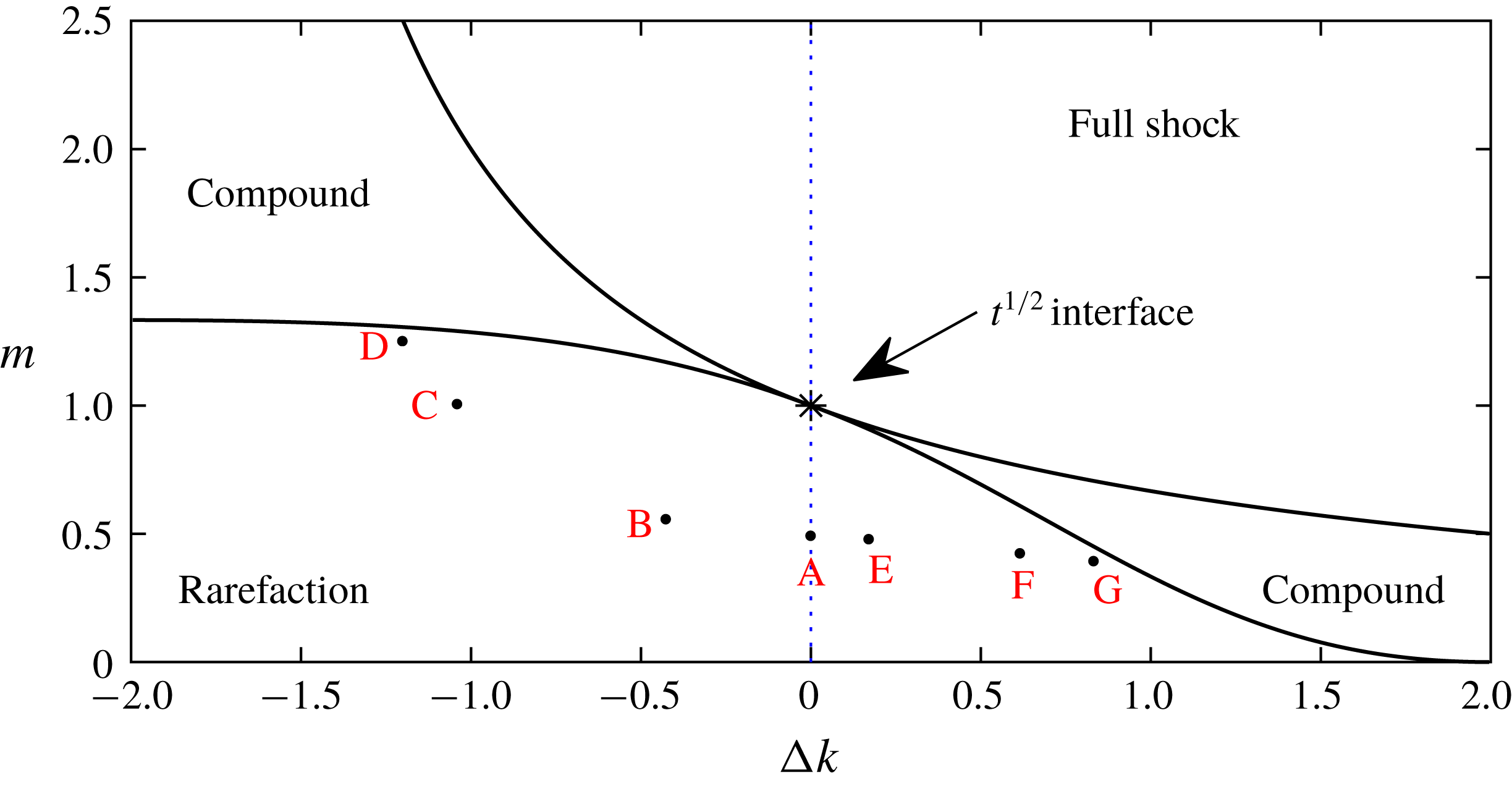
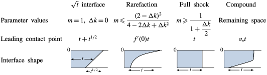
With this choice of permeability profile, the interface can evolve into one of four late-time regimes found by Hinton & Woods (Reference Hinton and Woods2018), depending on the values of the parameters
 $\unicode[STIX]{x0394}k$
and
 $m$
. The four regimes include generalisations of the three found for a uniform aquifer: a growing interface across the depth of the aquifer, a travelling wave of fixed extent and the singular case in which the interface grows in proportion to
 $t^{1/2}$
. The additional fourth regime, which does not occur in a uniform aquifer, consists of a shock region near the upper boundary, which travels with constant velocity
 $v_{s}$
, and a growing region below that which arises when the effect of the viscosity contrast and the permeability gradient act in opposition. The regimes are summarised in table 1, and shown in parameter space in figure 4.
Parameter space delineating the different regimes for the evolution of the interface in an aquifer with a permeability gradient (from Hinton & Woods Reference Hinton and Woods2018). The vertical axis is the viscosity ratio,
 $m=\unicode[STIX]{x1D707}_{i}/\unicode[STIX]{x1D707}_{a}$
, of the injected and ambient fluid. The left-hand side (
 $\unicode[STIX]{x0394}k<0$
) corresponds to the permeability increasing towards the top of the aquifer whilst the right-hand side corresponds to permeability decreasing towards the top of the aquifer. Four regimes can occur: a travelling wave of fixed extent (‘full shock’), a nose which grows in proportion to
 $t$
(a ‘rarefaction’ wave), a mixture of shock and rarefaction regions (‘compound’) and the singular case of isoviscous fluids in a uniform aquifer in which the nose grows in proportion to
 $t^{1/2}$
. The dashed blue line indicates
 $\unicode[STIX]{x0394}k=0$
, the case of uniform permeability. To understand the migration of tracer in the rarefaction regime, we consider the parameter values marked with red letters; the migration for A–D is shown in figure 5, and the migration of A, E–G is shown in figure 6.

Late-time shapes for injection into an aquifer with a permeability that varies linearly with depth, from Hinton & Woods (Reference Hinton and Woods2018). The regimes are distinguished in parameter space in figure 4.

The vertical shear produced when there is a vertical gradient of permeability can lead to fundamentally different regimes for the migration of tracer to those found for a uniform aquifer which we presented in § 2. The singular regime in which the interface grows in proportion to
 $t^{1/2}$
occurs only in a uniform aquifer. We now study the other three regimes in turn, beginning in § 4 with the migration of the tracer when the nose has the form of a growing rarefaction wave for which we identify three different subregimes depending on the viscosity ratio and the vertical permeability contrast. We then study the migration of the tracer in the full shock regime in § 5 and finally consider the compound regime in § 6.
4 Tracer migration in a growing nose in a heterogeneous aquifer
In this section, we study the migration of the tracer in the case that the nose of the current grows in proportion to
 $t$
and the permeability in the aquifer varies linearly with depth (see the second column in table 1). We generalise the results of § 2.3 which analysed the migration in a growing nose in a uniform aquifer. We first analyse the structure of the nose and flow therein, and then show that this leads to three subregimes for the evolution of the tracer.
4.1 Interface shape and flow structure in a growing nose
In the case of a linear permeability profile (3.8), Hinton & Woods (Reference Hinton and Woods2018) found that the condition for a growing nose,
 $f^{\prime \prime }(h)<0$
for all
 $h$
in
 $(0,1)$
, is equivalent to
 $$\begin{eqnarray}m\leqslant \frac{(2-\unicode[STIX]{x0394}k)^{2}}{4-2\unicode[STIX]{x0394}k+\unicode[STIX]{x0394}k^{2}}.\end{eqnarray}$$
When this condition is satisfied, the shape of the nose can be found implicitly from (3.5) by using the similarity variable
 $x/t$
,
 $$\begin{eqnarray}x(h,t)=f^{\prime }(h)t,\end{eqnarray}$$
where
 $$\begin{eqnarray}f^{\prime }(h)=\frac{mk(h)}{[m+(1-m)\unicode[STIX]{x1D713}(h)]^{2}}.\end{eqnarray}$$
The position of the trailing contact point,
 $h(x_{1}(t),t)=1$
, can be calculated from the equation for the shape of the nose (4.2),
 $$\begin{eqnarray}x_{1}(t)=f^{\prime }(1)t=mk(1)t.\end{eqnarray}$$
Similarly, the leading contact point,
 $h(x_{0}(t),t)=0$
, has position given by
 $$\begin{eqnarray}x_{0}(t)=f^{\prime }(0)t=k(0)t/m.\end{eqnarray}$$
The shape of the nose is controlled by two parameters, the viscosity ratio,
 $m$
, and the permeability gradient,
 $\unicode[STIX]{x0394}k$
. In the case of a uniform aquifer (
 $\unicode[STIX]{x0394}k=0$
) the position of the leading contact point was found to be
 $t/m$
. As the viscosity of the injectate decreases relative to the ambient fluid, the nose becomes elongated owing to the instability which occurs when a less viscous fluid is injected into a more viscous fluid (Saffman & Taylor Reference Saffman and Taylor1958). A permeability gradient across the aquifer may complement or oppose the effect of the viscosity ratio. If the permeability increases towards the top of the aquifer (
 $\unicode[STIX]{x0394}k<0$
), the injected fluid prefers to flow near the upper boundary and this enhances the effect of the viscous fingering (case B, figure 4). As the magnitude of the change in permeability increases, the role of the viscosity contrast becomes smaller in driving the instability (e.g. cases B and C, figure 4). Eventually, it is possible for the variations in permeability to dominate the spreading of the nose of the flow and in fact even if the viscosity gradient becomes weakly stabilising (
 $m>1$
), a sufficient gradient in the permeability can still lead to the spreading of the nose of the flow (case D, figure 4). In § 4.2, we analyse how the dispersal of tracer is influenced by this balance between the permeability gradient and the viscosity gradient, for flow regimes B–D.
In the opposite case that the permeability decreases towards the top of the aquifer (
 $\unicode[STIX]{x0394}k>0$
), we expect the extent of the finger to be reduced (case E, figure 4). If the permeability decreases sufficiently rapidly towards the top of the aquifer, then even with an unstable viscosity ratio the viscous fingering instability at the top of the domain may be suppressed.
To determine how tracer migrates within the nose, we calculate the horizontal and vertical velocities in the nose region from (3.4) and mass continuity,
 $$\begin{eqnarray}u(x,y,t)=\frac{k(y)}{m+(1-m)\unicode[STIX]{x1D713}(h)},\quad v(x,y,t)=\frac{(1-m)\unicode[STIX]{x1D713}(y)f^{\prime }(h)}{mf^{\prime \prime }(h)t},\end{eqnarray}$$
where
 $h=h(x,t)$
. As before, in the long-time limit, buoyancy is neglected. The velocities upstream of the nose are
 $u=k(y)$
and
 $v=0$
.
In the case that the fluids have equal viscosities (
 $m=1$
), the vertical velocity in the nose is zero and the flow is purely horizontal. Since
 $f^{\prime \prime }(h)<0$
and
 $f^{\prime }(h)>0$
, the vertical velocity is negative when
 $m<1$
and fluid migrates towards the upper boundary, whilst when
 $m>1$
, fluid migrates down towards the bottom boundary. This change in the flow structure is independent of the permeability gradient. Indeed,
 $m=1$
is a limiting case for any general nonlinear permeability profile. The limit of purely horizontal flow is critical to understanding the migration of tracer and will be used in our discussion below.
4.2 Permeability increasing towards the top of the aquifer (
$\unicode[STIX]{x0394}k<0$
)

Tracer migration in a growing nose in the case that the permeability decreases from top to bottom (
 $\unicode[STIX]{x0394}k<0$
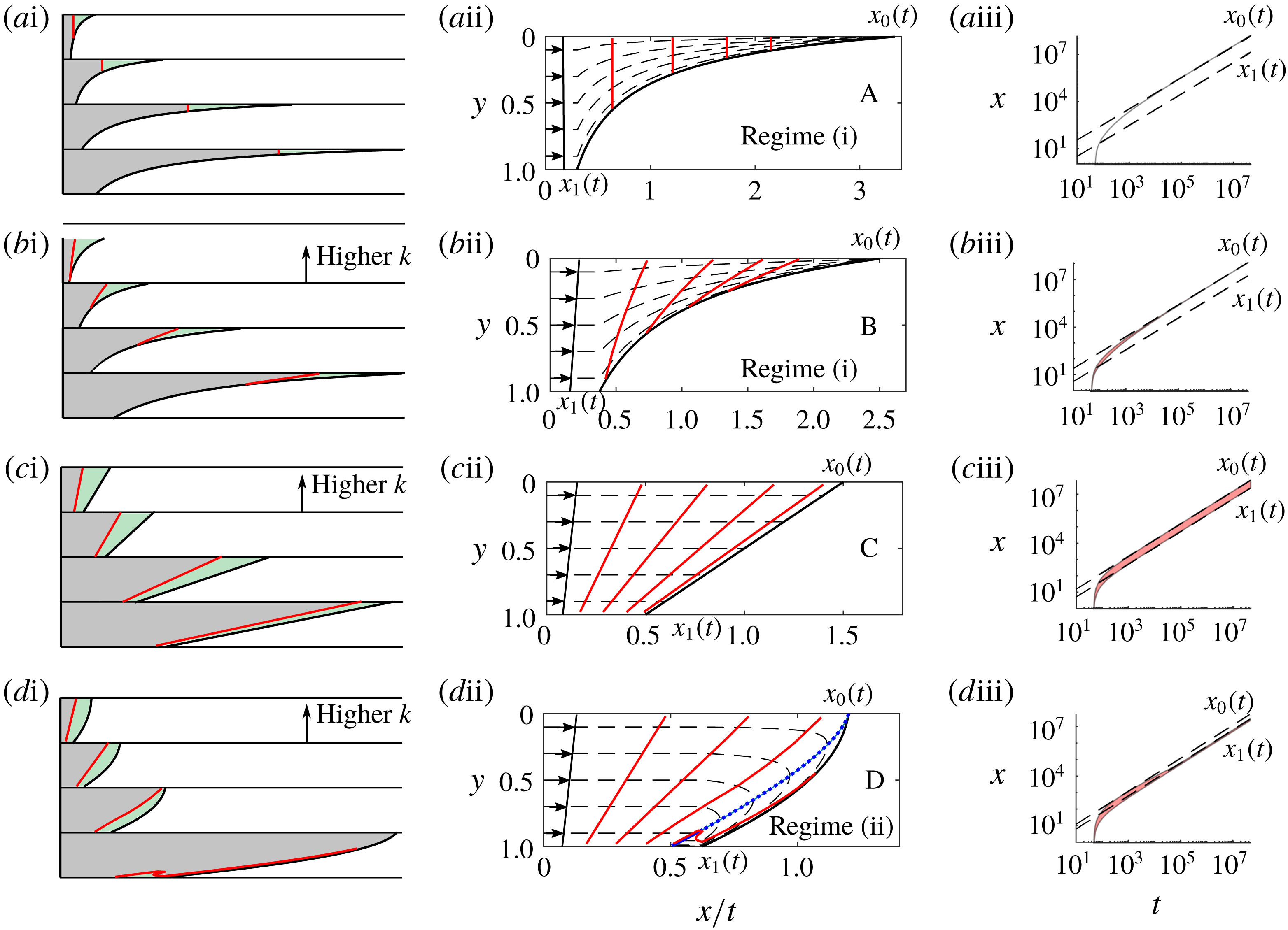
). Panels (ai–di) show how the tracer (red line) is carried into the nose in real coordinates at four times. The volume of the green fluid ahead of the tracer is constant. Panels (aii–dii) show the direction of the shear, the particle paths (dashed lines) relative to the growing nose and the position of the tracer at four times (red lines) corresponding to the times in the four cartoons. In panels (aiii–diii), the shaded area shows the along-channel positions occupied by a pulse of tracer released at
 $t_{R}=50$
, and the position of the contact points (dashed lines). The rows correspond to A–D in parameter space in figure 4. The case of a uniform aquifer is included in the top row for comparison. The dashed blue line in (dii) distinguishes the region in which fluid travels more slowly than the nose.

We examine the migration of tracer in the case that the permeability increases towards the top of the aquifer (
 $\unicode[STIX]{x0394}k<0$
) corresponding to cases B–D in figure 4.
In a uniform aquifer, the speed is constant with depth, and fluid enters the nose at all depths with the same flux. As the nose grows in time this fluid is then distributed through the nose, and as a result, the streamlines are all tilted upwards (see figure 5 aii). A line of tracer therefore moves into the nose and gradually enters shallower and shallower regions as the nose stretches out. If the permeability increases towards the top a small amount, this same process dominates, and the streamlines are all tilted upwards as in the uniform case. However, the speed on the higher streamlines is faster and so a line of tracer becomes stretched out laterally within the nose, with the leading part of the tracer being at the top of the aquifer (case B, figures 4, 5 b).
As the viscosity ratio,
 $m$
, is increased, the nose grows more slowly, reducing the tilting of the streamlines. A specific value is reached at which exactly the correct flux of fluid is supplied above each height to supply the growing nose region above that height, and so the streamlines are everywhere horizontal (case C, figures 4, 5
c). In this special case, the tracer is sheared out, but the tracer now remains on an inclined straight line. As discussed earlier, this corresponds to
 $m=1$
, and occurs for any permeability gradient which increases towards the top of the aquifer.
Finally, if the permeability increases sufficiently rapidly towards the top of the aquifer, but the effect of the viscosity is stabilising (
 $m>1$
) then the speed of the flow upstream of the nose can exceed the speed of the head of the nose near the upper boundary of the aquifer. As a result, fluid near the top of the aquifer travels faster than the front of the nose, and hence moves into the nose. However, the upstream speed in the aquifer at lower points is now smaller than the speed of the nose, and so here, the fluid at that depth cannot supply the nose region. Instead the fluid entering the nose at higher points in the aquifer moves down into the lower part of the nose region. Here, the speed is smaller than the speed of the nose, and so the fluid begins to lag behind the nose of the flow. The region in which particles travels more slowly than the nose is bounded by the interface and the dashed blue line in figure 5(dii). The dashed blue line is the nullcline on which the flow velocity equals the nose velocity. All the tracer eventually converges to a line of points behind the nose on which
 $x=k(y)t$
, shown as a solid blue line in figure 5(dii). To find the equation of the nullcline, we consider points in similarity space, i.e. (
 $x/t$
,
 $y$
) coordinates, at which the along-channel velocity is equal to the velocity of the nose,
 $$\begin{eqnarray}u(x,y,t)=f^{\prime }(h(x,t)).\end{eqnarray}$$
Using our expressions for
 $u$
and
 $f^{\prime }(h)$
(4.6) and (4.3), this can be rewritten as
 $$\begin{eqnarray}\frac{k(y)}{m+(1-m)\unicode[STIX]{x1D713}(h)}=\frac{mk(h)}{[m+(1-m)\unicode[STIX]{x1D713}(h)]^{2}}.\end{eqnarray}$$
Noting that the depth is a function only of
 $x/t$
so
 $h(x,t)=h(x/t)$
, the shape of the nullcline is given implicitly by
 $$\begin{eqnarray}y=\frac{m\unicode[STIX]{x0394}kh-(1-m)\unicode[STIX]{x1D713}(h)k(0)}{m\unicode[STIX]{x0394}k+(1-m)\unicode[STIX]{x1D713}(h)\unicode[STIX]{x0394}k},\end{eqnarray}$$
where
 $h=h(x/t)$
. Note that this line coincides with the interface in the limiting case of
 $m=1$
.
We have found two regimes for the migration of the tracer. We call the case in which the tracer migrates into continually shallower regions of the nose ‘regime (i)’ (A and B in figure 5), and the case in which the tracer enters the nose in the high permeability region at the top of the aquifer and subsequently lags behind the nose in the low permeability region ‘regime (ii)’ (D in figure 5). The migration towards the leading contact point in regime (i) and migration behind the trailing contact point in regime (ii) is illustrated in figure 5(aiii–diii); the shaded area shows the along-channel positions of the tracer and the dashed lines are the positions of the contact points.
4.3 Permeability increasing towards the bottom of the aquifer (
$\unicode[STIX]{x0394}k>0$
)

Tracer migration in a growing nose in the case that the permeability increases towards the bottom of the aquifer (
 $\unicode[STIX]{x0394}k>0$
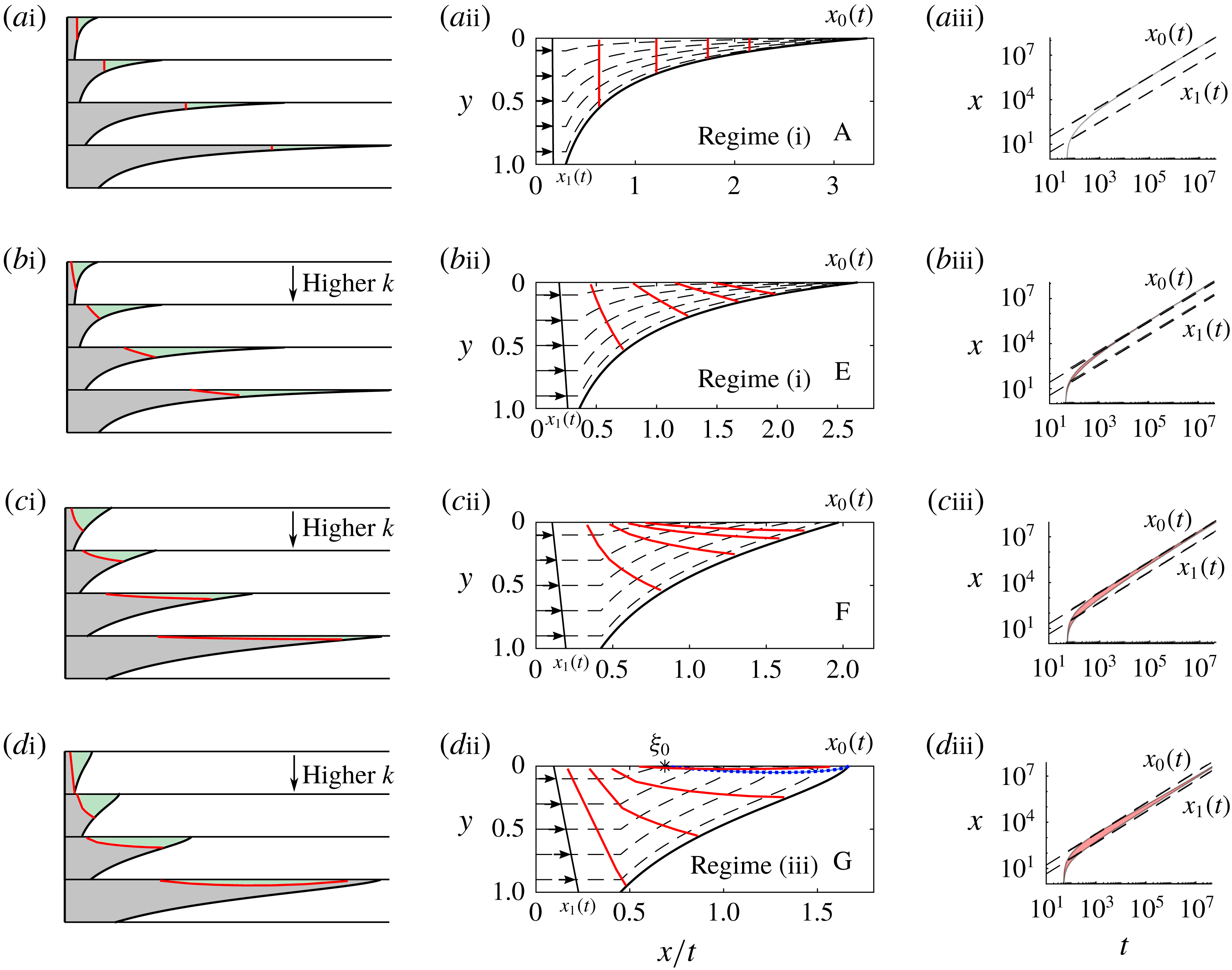
). Panels (ai–di) show how the tracer (red line) is carried into the nose in real coordinates at four times. The volume of the green fluid ahead of the tracer is constant. Panels (aii–dii) show the direction of the shear, the particle paths (dashed lines) relative to the growing nose and the position of the tracer at four times (red lines) corresponding to the times in the four cartoons. In panels (aiii–diii), the shaded area shows the along-channel positions occupied by a pulse of tracer released at
 $t_{R}=50$
, and the position of the contact points (dashed lines). The rows correspond to A, E, F and G in parameter space in figure 4. The case of a uniform aquifer is included in the top row for comparison. The dashed blue line in (dii) distinguishes the region in which fluid travels more slowly than the nose, and
 $\unicode[STIX]{x1D709}_{0}$
is the position along the upper boundary which tracer converges to in similarity coordinates.

We examine the migration of tracer in the case that the permeability is highest towards the bottom of the aquifer (
 $\unicode[STIX]{x0394}k>0$
) corresponding to cases E–G in figure 4. Note that the viscosity ratio is less than
 $1$
in this case because the permeability gradient suppresses the viscous fingering. Hence,
 $v<0$
(see (4.6b
)) and fluid in the nose always migrates upwards.
If there is a small increase in permeability from the top of the aquifer to the bottom then the streamlines are all tilted upwards as in the uniform case. However, the speed on the lower streamlines is faster and so a line of tracer becomes stretched out laterally within the nose, with the leading part of the tracer being nearest to the interface (case E, figures 4, 6 b). Tracer migrates into shallower and shallower regions as the nose stretches out and hence case E lies in regime (i) (see figure 6 biii).
In an aquifer with a larger increase in permeability from the top to the bottom, the fluid near the bottom of the aquifer travels much faster than the nose. There is a specific value, which shall be specified later in (4.11), at which the lower region provides sufficient flux that the leading portion of the nose is supplied only by fluid from the bottom of the aquifer. In this case, fluid near the top of the aquifer does not migrate into continually shallower regions of the nose; instead, particles travel towards the top boundary and subsequently slowly converge towards the leading contact point (case F, figures 4, 6 c).
If the permeability increase is even larger, the flux entering the nose near the bottom boundary is greater than the flux needed to supply the growing nose. Owing to mass conservation, fluid reverses relative to the nose in a thin region near the upper boundary (case G, figures 4, 6
d). The equation of the nullcline is given by (4.9). We call this ‘regime (iii)’. It is fundamentally different from regime (ii) because fluid is supplied to the nose from the bottom of the aquifer, and fluid never lags behind the nose. The nullcline intersects the upper boundary at a point
 $\unicode[STIX]{x1D709}_{0}$
given implicitly by
 $$\begin{eqnarray}h(\unicode[STIX]{x1D709}_{0})=\frac{2m}{(1-m)k(0)}+1-\frac{2}{\unicode[STIX]{x0394}k}.\end{eqnarray}$$
Tracer converges towards a region around this point which lies within the nose, and between the two contact points (see figures 6 dii and 6 diii).
To find the value of the viscosity ratio at which the transition between regimes (i) and (iii) occurs, we analyse the limiting case (F in figures 4, 6c). Fluid migrates towards the upper boundary and the nullcline just touches the upper boundary. This corresponds to the stationary point given by (4.10) coalescing with the leading contact point. Setting
 $h(\unicode[STIX]{x1D709}_{0})=0$
yields
 $$\begin{eqnarray}m=\frac{(2-\unicode[STIX]{x0394}k)^{2}}{\unicode[STIX]{x0394}k^{2}+4},\end{eqnarray}$$
which is the boundary between regime (i) and regime (iii).
It is interesting to note that the regimes correspond to the convexity of the interface at the leading contact point. The interface is concave for parameter values in regime (i), and convex at the leading contact point for regimes (ii) and (iii). The limiting interface between regimes (i) and (ii) is linear and the limiting interface between regimes (i) and (iii) has an inflection point at the leading contact point (see figures 5 cii and 6 cii). This characterisation arises from the linear shear; the limiting regimes occur when the interface is linear because the volume of fluid supplied at each height upstream of the nose matches the flux at that height in the nose. If the permeability gradient was not linear, the limit between regimes would not correspond to a locally linear interface at the leading contact point.
4.4 Dispersion coefficients
The lateral extent of the tracer could be used to constrain aquifer properties. In a growing nose our results imply that the rate of longitudinal dispersion at late times depends critically on the regime. In regime (i), in which the tracer migrates into progressively shallower regions of the nose, the lateral extent of the tracer increases at a rate slower than
 $t$
because the influence of the permeability gradient diminishes as the tracer migrates into shallower regions (see figure 6
bii). In regime (ii), the tracer converges to a line of points upstream of the nose near the lower boundary (see figure 5
dii). The equation of this line is
 $x=k(y)t$
for
 ${\hat{y}}\leqslant y\leqslant 1$
where
 ${\hat{y}}=(mk(1)-k(0))/\unicode[STIX]{x0394}k$
is the depth of the line at the trailing contact point. The extent of this line grows in proportion to
 $t$
and the horizontal standard deviation of the tracer is
 $$\begin{eqnarray}\langle (x-\bar{x})^{2}\rangle ^{1/2}=\frac{(m-1)k(1)t}{2\sqrt{3}}.\end{eqnarray}$$
In regime (iii), the tracer migrates towards a region near the upper boundary and hence samples a progressively smaller portion of the permeability contrast. Therefore, at long times, the extent of the tracer in the nose increases more slowly than
 $t$
(see figure 6
diii). Note that the rate of dispersion at early times, before the tracer enters the nose, is proportional to
 $|\unicode[STIX]{x0394}k|t$
in each regime owing to the linear permeability contrast across the aquifer.
5 Heterogeneous aquifer: tracer migration in a nose of fixed extent
We now consider the case in which the nose is a travelling wave of fixed extent (see third column of table 1), then in § 6, we will combine the results from the present and preceding sections to investigate the flow in the case that the nose has regions which grow and regions of fixed extent.
We first investigate the shape of the nose region and the flow structure. Hinton & Woods (Reference Hinton and Woods2018) found the condition for a travelling wave across the aquifer to be
 $$\begin{eqnarray}m\geqslant \frac{1}{1+{\displaystyle \frac{\unicode[STIX]{x0394}k}{2}}}.\end{eqnarray}$$
In this case, the governing equation (3.3) has a travelling-wave solution which travels with constant shape and the velocity of the mean flow. By transforming to coordinates moving with the front,
 $\unicode[STIX]{x1D702}=x-t$
, Hinton & Woods (Reference Hinton and Woods2018) found the shape of the interface satisfies
 $$\begin{eqnarray}\frac{\text{d}h}{\text{d}\unicode[STIX]{x1D702}}=\frac{\unicode[STIX]{x1D713}(h)-mh+(m-1)h\unicode[STIX]{x1D713}(h)}{m\unicode[STIX]{x1D713}(h)(1-\unicode[STIX]{x1D713}(h))}.\end{eqnarray}$$
Using the Darcy velocity (3.4), and mass continuity, we can calculate the horizontal and vertical particle velocities in the nose region,
 $$\begin{eqnarray}u=\frac{h}{\unicode[STIX]{x1D713}(h)}k(y),\quad v=-\unicode[STIX]{x1D713}(y)\frac{\unicode[STIX]{x1D713}(h)-hk(h)}{\unicode[STIX]{x1D713}(h)^{2}}\frac{\text{d}h}{\text{d}\unicode[STIX]{x1D702}}.\end{eqnarray}$$
Upstream of the nose, in the fully flooded region,
 $u=k(y)$
and
 $v=0$
. There is a discontinuity in
 $v$
at the trailing contact point. This is unphysical but the hydrostatic assumption requires that
 $b\ll 1$
(see (2.14)) meaning the horizontal length scale is much larger than
 $H_{0}$
and hence in dimensional terms the vertical velocity is much less than the horizontal velocity and the discontinuity in the vertical velocity is small.
In § 2.5, we showed that in a uniform aquifer in which there is a travelling-wave solution, all the fluid travels at the mean flow speed and a line of tracer remains a fixed distance behind the nose. Now, when the aquifer is not uniform, the variation of the permeability with height partitions the line of tracer into heights where the tracer travels faster than the mean speed (
 $k(y)>1$
) and heights where the tracer is slower (
 $k(y)<1$
). The vertical line of tracer is linearly sheared until the fastest particle, either
 $y=1$
if
 $\unicode[STIX]{x0394}k>0$
or
 $y=0$
if
 $\unicode[STIX]{x0394}k<0$
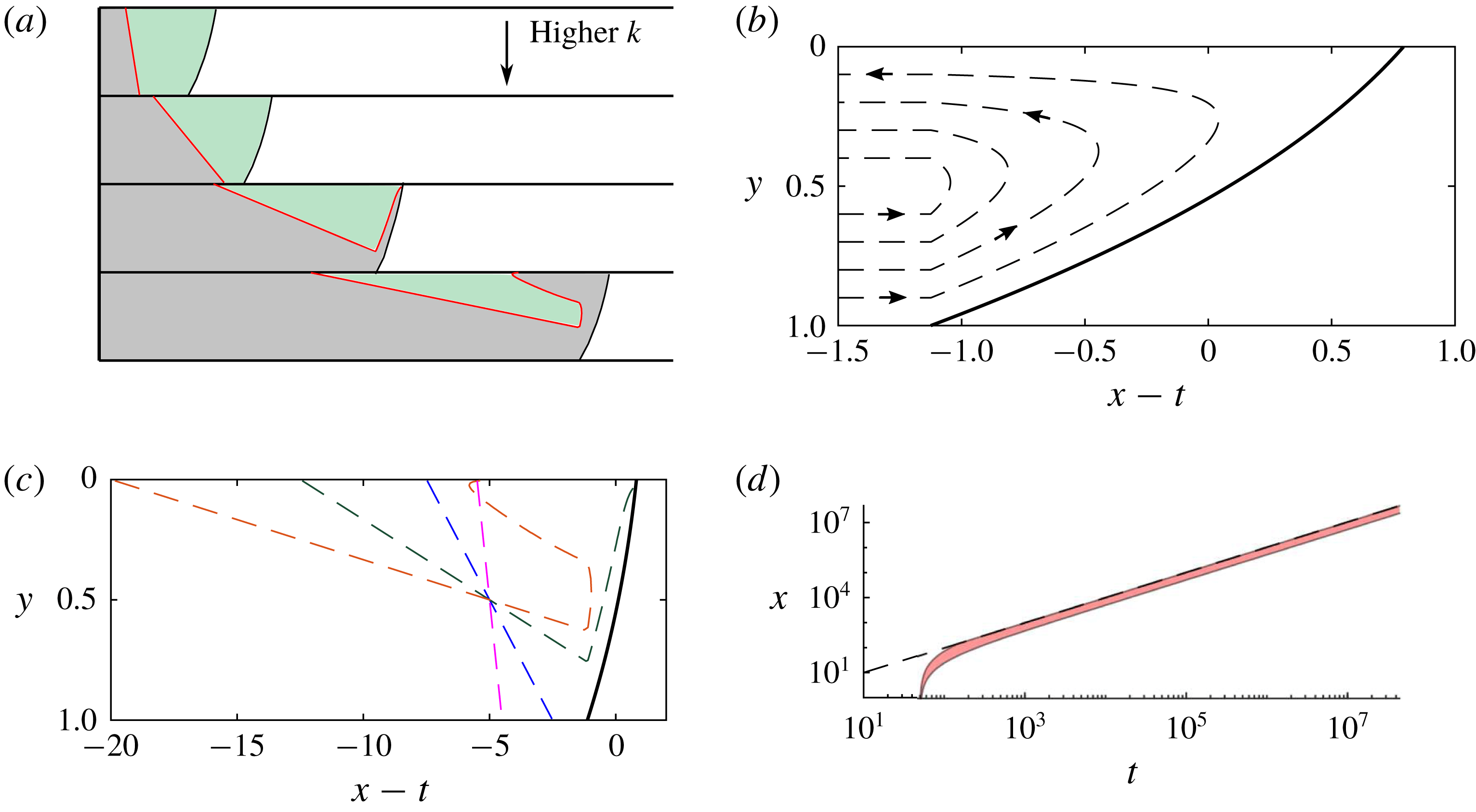
reaches the nose region which travels at the mean speed. This fastest particle enters the nose, and travels across the aquifer towards the lower permeability region near the opposite boundary of the aquifer where it is left behind by the advancing nose region (see figure 7). After the first entry time, the tracer at progressively lower (or greater if
 $\unicode[STIX]{x0394}k<0$
) heights reaches the nose region where it travels to successively higher (or lower) points in the slower half. This eventually leads to the migration of all particles which originate in the region in which
 $k(y)>1$
to the region in which
 $k(y)<1$
, the slow half. In contrast, particles which began in the slow region never reach the nose. These particles undergo a linear shear. The particle at
 $y=1/2$
travels at the speed of the nose. At long times, there are then two regions of tracer: that which has travelled through the nose and that which has not. Both are linearly sheared and form lines joining the slow boundary of the aquifer to the point at
 $y=1/2$
behind the nose. The initial vertical line of tracer has been folded in half and linearly sheared as shown in figure 7 for the case of permeability decreasing towards the top of the aquifer (
 $\unicode[STIX]{x0394}k>0$
). Figure 8 shows the case
 $\unicode[STIX]{x0394}k<0$
. The particle paths and interface shape are calculated numerically using (5.2) and (5.3). Owing to mass conservation, particles that enter the nose at
 $y=y_{0}$
leave at
 $y=1-y_{0}$
.
The interaction between the shearing of the tracer and a fixed nose. The permeability increases from the top of the aquifer to the bottom of the aquifer (
 $\unicode[STIX]{x0394}k>0$
). (a) A cartoon illustrating how a red line of tracer undergoes a shear, tracer in the fast regions enters the nose and subsequently encloses the green fluid which was initially ahead of the line of tracer. Panel (b) shows particle paths relative to the travelling nose, particles below
 ${\textstyle \frac{1}{2}}$
are deflected into the upper region. Panel (c) shows the position of a line of tracer at four times (dashed lines) relative to the position of the interface (solid line). The line of tracer is folded over itself and becomes two asymptotically parallel lines joining the top of the aquifer to the trailing edge of the nose. (d) The position of a pulse of tracer relative to the leading contact point (dashed line) illustrating that the tracer disperses at a rate proportional to
 $t$
.

Tracer migration for permeability increasing towards the top of the aquifer (
 $\unicode[STIX]{x0394}k<0$
), in the case of a fixed nose. (a) A cartoon illustrating how a red line of tracer undergoes a shear, tracer in the fast regions enters the nose and subsequently encloses the green fluid which was initially ahead of the line of tracer. Panel (b) shows particle paths relative to the travelling nose; particles above
 $1/2$
are deflected into the lower region. The late-time evolution of a line of tracer is similar to the case
 $\unicode[STIX]{x0394}k>0$
up to a reflection across
 $y=1/2$
.

At times long after all the tracer is in the slow half of the aquifer, the two lines of tracer continue to be linearly sheared and become asymptotically identical straight lines with gradient
 $(\unicode[STIX]{x0394}kt)^{-1}$
. The distance behind the front of the centre of mass of the tracer tends to
 $$\begin{eqnarray}\frac{\unicode[STIX]{x0394}kt}{4}\end{eqnarray}$$
as
 $t\rightarrow \infty$
. Similarly, the horizontal standard deviation of the tracer is
 $$\begin{eqnarray}\frac{\unicode[STIX]{x0394}kt}{4\sqrt{3}}.\end{eqnarray}$$
The extent of tracer grows in proportion to
 $t$
and
 $\unicode[STIX]{x0394}k$
owing to the shear, in contrast to a uniform aquifer in which there is no dispersion. Molecular diffusion or pore-scale dispersion would lead to growth in the extent of the tracer zone at a rate proportional to
 $t^{1/2}$
in a uniform flow (cf. Phillips Reference Phillips2009).
6 Heterogeneous aquifer: tracer migration in a nose with a growing and a fixed region
In this section, we investigate how tracer migrates in a compound nose involving a region which grows in proportion to
 $t$
and a region in which there is a travelling wave of fixed extent with height
 $h_{s}$
and constant velocity
 $v_{s}$
. We show that the evolution of a pulse of tracer is similar to that in regime (ii) (see § 4.2). In regions of higher permeability the tracer travels faster than the nose. Upon entering the nose this tracer migrates across the aquifer into lower permeability regions and subsequently lags behind the advancing nose (see figure 9). The details of the migration within the nose are altered from the case of regime (ii) by the fixed region at the front of the nose.
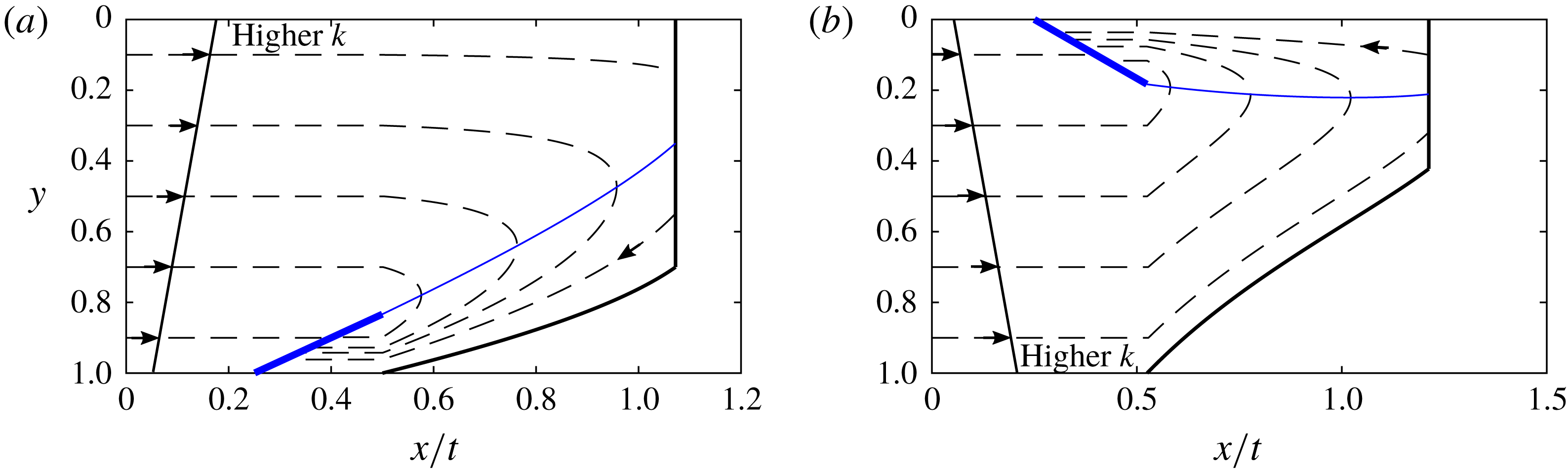
Evolution of the tracer in a compound nose. Particle paths (dashed) and the interface (solid) are shown in
 $x/t$
coordinates. The nullcline along which the flow velocity equals the local velocity of the interface is a thin blue line whilst the thick blue line behind the nose region is the line of points which particles converge to. The shock region has constant shape. (a) The case where the permeability is higher towards the top of the aquifer (
 $\unicode[STIX]{x0394}k<0$
). (b)
 $\unicode[STIX]{x0394}k>0$
.

Figure 9(a) shows the case
 $\unicode[STIX]{x0394}k<0$
, where the permeability increases towards the top of the aquifer. A line of tracer upstream of the nose is partitioned into three regions by height according to the flow velocity. In the top region, the velocity is highest and fluid enters the growing nose and migrates into the fixed region. In the fixed region, particles travel across the nose into lower permeability regions and subsequently lag behind the fixed region. The flow within the fixed region is as described in § 5, with the velocities increased by a factor
 $v_{s}$
, the velocity of the fixed region. After migrating through the fixed region the tracer continues to travel more slowly than the nose and lags behind the nose and towards the line of constant velocity on which
 $x=k(y)t$
(shown as a thick blue line in figure 9). Tracer in the second region, in the middle of the aquifer, travels fast enough to enter the nose but not fast enough to enter the fixed region. This tracer migrates across the aquifer within the growing region, it crosses the nullcline (thin blue line in figure 9) and subsequently lags behind the nose towards the line of constant velocity. Finally, tracer initially near the bottom of the aquifer lies in the region of lowest permeability and never enters the nose. Instead this tracer converges towards the line of constant velocity from upstream. Figure 9(b) shows the case
 $\unicode[STIX]{x0394}k>0$
which is similar. Note that a smaller viscosity ratio,
 $m$
leads to a shallower fixed region.
In the case that the permeability is highest towards the top of the aquifer (
 $\unicode[STIX]{x0394}k<0$
), the rate of dispersion of tracer at late times is the same as in regime (ii),
 $$\begin{eqnarray}\frac{(m-1)k(1)t}{2\sqrt{3}},\end{eqnarray}$$
because tracer converges to the same line of constant velocity as in regime (ii) (see thick blue line in figure 9
a). In the case that the permeability is lowest towards the top of the aquifer (
 $\unicode[STIX]{x0394}k>0$
), the line to which tracer converges at late times is
 $x=k(y)t$
at the top of the aquifer (see thick blue line in figure 9
b). The standard deviation is adjusted to
 $$\begin{eqnarray}\frac{(mk(1)-k(0))t}{2\sqrt{3}}.\end{eqnarray}$$
7 Conclusion
We have analysed the migration of tracer within a flow in a confined aquifer in which the permeability varies linearly with height. In the context of
 $\text{CO}_{2}$
sequestration, our work focuses on the regime in which the dispersion of the tracer by the shear dominates the effects of pore-scale dispersion or molecular diffusion. In this regime, the tracer evolution is controlled by the structure of the leading interface of the
 $\text{CO}_{2}$
plume as well as the shear.
For reference, we have shown that in a uniform medium the nose region may either grow in time if the viscosity of the input fluid is less than the original, and it has a fixed shape if the viscosity of the input fluid is greater. If the nose region is growing, the tracer travels into increasingly shallow regions of the nose. If the nose region has fixed shape, the tracer remains a constant distance behind the interface.
When the formation has a vertical gradient of permeability, we have found three regimes for the evolution of the tracer in a growing interface: the tracer can continue to migrate into progressively shallower regions of the nose indefinitely; the tracer can enter the nose, and then circulate through the nose, so that it then reverses relative to the interface and drops out of the nose; finally, the tracer may converge to a region within the nose. We have found parameter values which delineate these different regimes and explored the transitions between them.
The combination of a shear flow and a fixed-shape, shock-like interface also leads to novel results. Fluid in the high permeability regions travels faster than the interface, this fluid enters the nose and subsequently migrates out of the nose via the low permeability region. The longitudinal extent of the tracer then grows in proportion to
 $t$
, rather than
 $\sqrt{t}$
which would be expected if small-scale dispersion or diffusion dominated. In the cases where the lateral extent of tracer grows in proportion to
 $t$
we have found the long-time dispersion coefficients. It may be possible to use these coefficients to constrain the structure of the permeability of an aquifer if the time interval over which tracer arrives at a production well is known.
In all regimes, the rate of longitudinal dispersion of the tracer is proportional to
 $|\unicode[STIX]{x0394}k|t$
at early times before tracer enters the nose. This picture has some similarities with the review of field data by Gelhar, Welty & Rehfeldt (Reference Gelhar, Welty and Rehfeldt1992) who investigated an extensive range of tracer dispersal data in water saturated aquifers, for which the viscosity ratio is unity, and found that the dispersion coefficient increased linearly with the distance between the wells. However, we note that in the real rock systems studied by Gelhar et al. (Reference Gelhar, Welty and Rehfeldt1992) the detailed permeability structure would be more complex than the present modelling, the flows are three dimensional and the effects of multiple layers may also play a role.
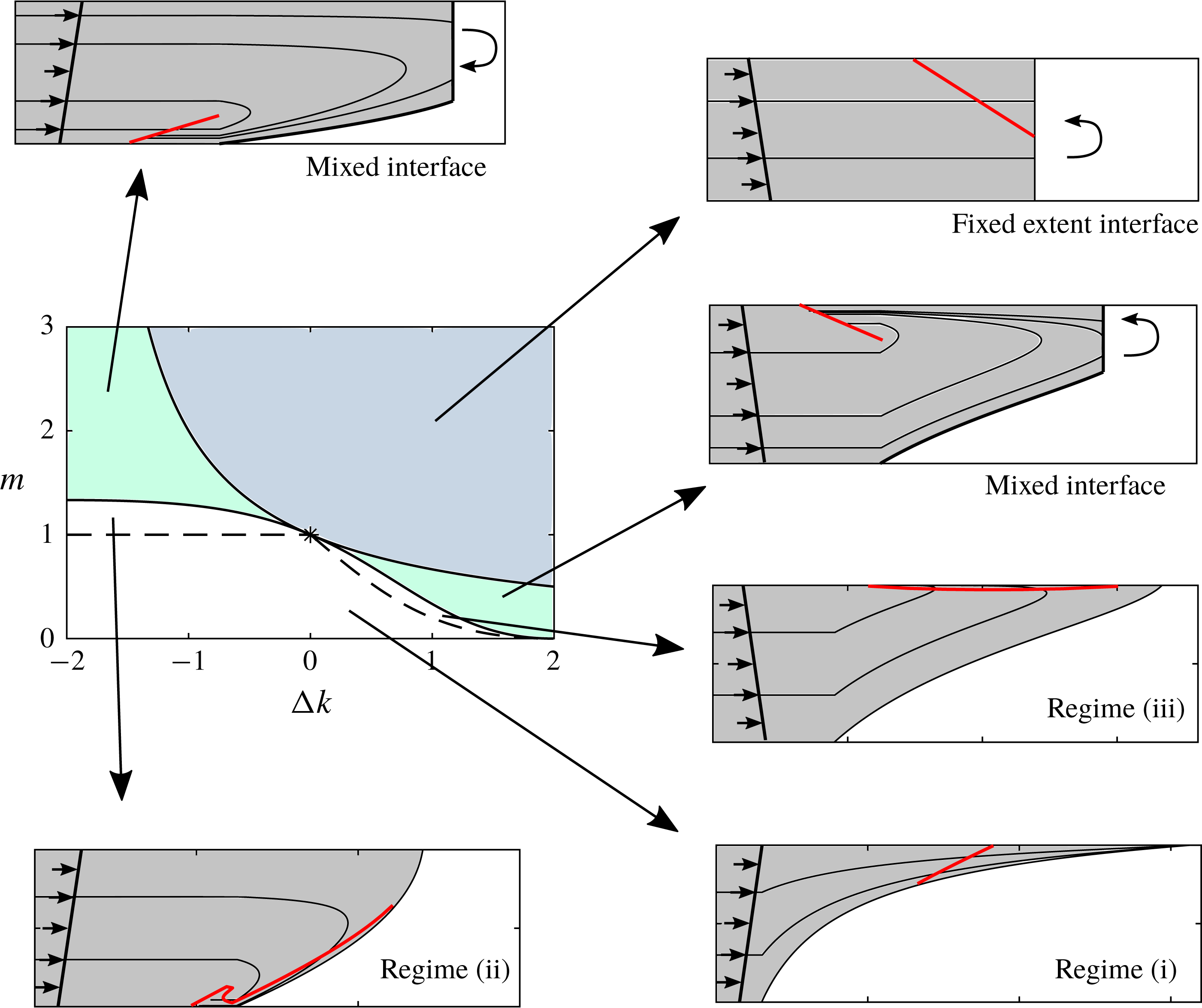
Parameter space and corresponding plots of the interface and flow structure in
 $x/t$
coordinates. The red lines show the position of the tracer at a late time. The dashed lines in parameter space separate the three regimes for a growing nose, and the boundary is given by
 $m=1$
in
 $\unicode[STIX]{x0394}k<0$
and (4.11) in
 $\unicode[STIX]{x0394}k>0$
. The curly arrows indicate the recirculation within the fixed extent regions.

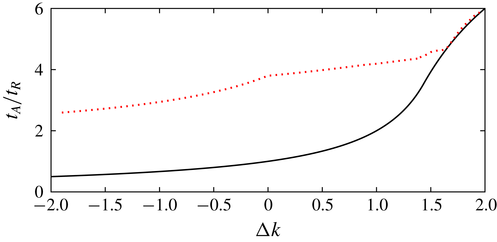
Arrival times of
 $\text{CO}_{2}$
(black continuous line) and tracer (red dashed line) at a producer well at
 $x=10$
.

In figure 10, we summarise the results of this paper and relate them to parameter space. The interface shapes in figure 10 are shown in
 $x/t$
coordinates and hence the fixed regions have zero width and the recirculation within them is not shown.
In future work, we plan to study how our model could be applied to invert the results of tracer tests to constrain aquifer parameters in the context of
 $\text{CO}_{2}$
sequestration. To briefly illustrate the complex relation between the permeability gradient and the results of tracer tests, we consider a simple tracer test. In our example, there is a producer well at
 $x=10$
, we take the typical value
 $m=0.1$
and consider releasing a tracer at
 $t_{R}=1$
from an injection well at
 $x=0$
, into which
 $\text{CO}_{2}$
was injected for time
 $t>0$
. We then calculate the time at which
 $\text{CO}_{2}$
and the tracer first arrive at the well as a function of the permeability gradient, shown in figure 11 by the continuous black and dashed red lines respectively.
As the permeability gradient is reduced, the permeability at the top of the aquifer increases and hence the
 $\text{CO}_{2}$
travels more quickly. For the arrival of the tracer, there is a change in behaviour at
 $\unicode[STIX]{x0394}k=0$
. The region in which the tracer travels the fastest changes from being the tracer at the top of the aquifer (
 $\unicode[STIX]{x0394}k<0$
) to the tracer travelling fastest at the bottom (
 $\unicode[STIX]{x0394}k>0$
). If the permeability gradient is sufficiently large, then a mixed shock–dispersive interface develops, and the delay between the arrival of
 $\text{CO}_{2}$
and tracer is reduced dramatically because tracer catches the nose much more quickly (cf. § 6). If the distance to the producer well were greater, the tracer would have time to fall behind the nose and the delay would increase at a larger permeability gradient.
The richness in the relative times of arrival of the tracer and the leading edge of the plume as a function of the permeability gradient in the cross-flow direction, as predicted by the model presented in this work, provides a framework to interpret tracer tests. Since it is difficult to access the detailed spatial distribution of subsurface reservoirs, interpretation of such tracer tests may be key in constraining models of the structure of the system. The inversion of real field data using simplified models as presented herein, involves a number of further challenges, including accounting for the presence of noise in the data, and for the non-ideal structure of real rocks. However, such models can provide very useful constraints on the flow properties, and we plan to explore this further in future work.
Acknowledgements
The authors wish to thank T. Espie for his support of this work, and BP and EPSRC for the award of a CASE studentship funding the research.
Appendix A. The significance of diffusion
The significance of small-scale dispersion or molecular diffusion on the motion of the tracer can be assessed by consideration of the ratio of the diffusive time scale and the advective time scale,
 $$\begin{eqnarray}\unicode[STIX]{x1D706}=\frac{T_{D}}{T_{A}}=\frac{L^{2}/D}{L/V_{0}},\end{eqnarray}$$
where
 $D$
is the coefficient of molecular diffusion for the tracer,
 $V_{0}=Q/(\unicode[STIX]{x1D719}H_{0})$
is the velocity at injection and
 $L$
is the length scale, which we take to be the depth of the aquifer,
 $H_{0}$
. In terms of the aquifer parameters, the ratio (A 1) is
 $$\begin{eqnarray}\unicode[STIX]{x1D706}=\frac{Q}{\unicode[STIX]{x1D719}D}.\end{eqnarray}$$
Buoyancy does not influence this ratio because at late times the flow is controlled by the injection pressure rather than buoyancy forces. If
 $\unicode[STIX]{x1D706}\gg 1$
, advection dominates until late times, and if
 $\unicode[STIX]{x1D706}\ll 1$
, diffusion is important even at earlier times.
In the context of
 $\text{CO}_{2}$
sequestration, using typical values of the injection flux,
 $Q=10^{-5}{-}10^{-4}~\text{m}^{2}~\text{s}^{-1}$
, and the porosity of the aquifer,
 $\unicode[STIX]{x1D719}=0.15$
, and assuming the diffusion coefficient,
 $D$
, is of order
 $10^{-9}~\text{m}^{2}~\text{s}^{-1}$
, the ratio is
 $$\begin{eqnarray}\unicode[STIX]{x1D706}=10^{4}{-}10^{5}.\end{eqnarray}$$
The pore-scale dispersion of tracer is therefore small compared to the influence of the shear on the dispersal and growth of the tracer zone.
In the present work, we have neglected the possible dissolution of
 $\text{CO}_{2}$
into the ambient brine (Riaz et al.
Reference Riaz, Hesse, Tchelepi and Orr2006; Neufeld et al.
Reference Neufeld, Hesse, Riaz, Hallworth, Tchelepi and Huppert2010). Such dissolution would reduce the velocity of the nose of the current. The mechanisms of tracer dispersion discussed in this work would still occur if dissolution were incorporated in the motion of the
 $\text{CO}_{2}$
, but in this case, a fraction of the tracer-laden
 $\text{CO}_{2}$
may dissolve into the brine, and this will then be lost from the
 $\text{CO}_{2}$
plume. It would be of interest to develop the model further to account for such dissolution, although we note that since
 $\text{CO}_{2}$
is only soluble in water up to a few per cent by mass. The dissolution would lead to a relatively slow evolution of the tracer mass, and only that part of the tracer which enters the head region of the flow and comes into contact with the leading edge of the flow would migrate into the brine.