

Introduction
Appropriately selecting maturity groups based upon planting date and soil characteristics can have a significant impact on yield. However, maturity groups also play a role in harvest logistics and the demand for drying and storage equipment. This demand for drying and storage also drives decisions of how crops are marketed. Economically, optimal decision making throughout this system manifests itself in maximum net returns. Furthermore, depressed grain prices have put pressure on farmers to improve their management and marketing strategies. One way to improve profitability is through the production of a specialty grain such as white food-grade corn. While processors will pay a premium for specialty grains, it is usually the case that they have strict quality standards that ultimately determine the price. Hence, producers must take considerable care in the harvest, dry down, and storage of specialty grains. This usually necessitates priority for the specialty grain to be harvested, dried and stored ahead of less valuable grain types. Ultimately, this can implicate decision making for other crops from planting to marketing. Additionally, the capacity of drying and storage equipment dictates how producers take advantage of the futures market, a strong margin between the local cash price and futures price, or opportunities like specialty grain production. Analysis can be performed on these capacities to determine if the equipment being used is under or oversized compared to production and what effect that has on returns.
The purpose of this paper is, therefore, to model net returns at the whole-farm scale based on the optimal combination of planting date, maturity group selection, and a differential marketing strategy for a production system typical of rainfed grain farms in western Kentucky. The model farm has an enterprise mix of white corn, corn, and soybeans over an area of 1040 hectares and two possible marketing strategies, cash and contract sales. Possible site-specific agronomic decisions revolve around the choice of variable maturity group cultivar selection planted into different topsoil depths. The proposed model then determines how production from different combinations and fixed drying and storage infrastructure affects potential marketing strategies and net returns. Constraints affecting this combination of variables include land, labor, yield, dryer and storage capacities, contract sale of white corn, and soil variation. Likewise, the demand for drying and storage of grain for futures contract sales will be analyzed for bottlenecks or slacks and the effect it has on net returns.
Materials and Methods
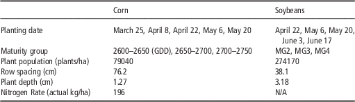
Linear programming is used to optimize the detailed whole farm plan. Microsoft Excel and Solver add-in are used to organize the tableau and compute maximized net returns using the Simplex method (Dantzig, Reference Dantzig1963). Essentially, there are two broad decision variable components in the tableau: production and marketing. For production, separate matrices are used for each crop and respective cultivar and planting date. These contain relevant constraint information such as yield potential and labor requirements per hectare. Marketing decisions are indexed by two categories, cash, and contract sales, and each of these contains matrices for each crop with applicable constraints (e.g. white corn contract, drying and storage capacities). Five planting date options are considered for all three crops. For white corn and corn, planting can take place March 25, April 8, April 22, May 6, or May 22. For soybeans, planting dates are April 22, May 6, May 20, June 3, and June 17. It should be noted that these dates represent a two-week window in which planting of a particular crop and its related maturity group(s) takes place. It is assumed the operation has the necessary technology to complete variable maturity group planting over different topsoil depths.
This study considers three maturity groups for both corn and soybeans which can be referenced in Table 1. A single maturity group (maturity group 2, 2650–2700 GDD) represents white corn production because of yield data limitations. Varying corn and soybean maturity groups among fields, and in this case by topsoil depth, can enable producers to lengthen planting and harvesting windows. Fields can be sequentially harvested as they mature which in turn minimizes yield loss from delayed harvest. Scheduling harvest operations around an optimal combination of maturity groups can also maximize the additional profit realized by using fixed drying and storage equipment to capture price premiums. This is due to the fact one maturity group can be dried and stored before another is ready to be harvested; alleviating bottlenecks and larger amounts of grain entering the (potentially) less profitable cash market. Two topsoil depths, deep and shallow, constitute 80% and 20% of the tillable hectares, respectively. These proportions are representative of soil characteristics in Henderson County, KY (NRCS, 2008). Soil variability based upon constituents such as sand, silt, and clay was not modeled due to computational constraints of Solver software and is recognized as a limitation.

Marketing strategies include spot cash sales and futures contract sales. Futures contract sales imply that a predetermined amount of either corn or soybeans is delivered in a specific month under terms established by buyer and seller where price is determined by the exchange where trading is conducted. In this instance, the exchange in which price data is gathered is the Chicago Mercantile Exchange (CME). Within the model, production allocated to cash sales is assumed to be harvested and transported directly to a commercial elevator with no on-farm drying or storage required. Essentially, this means the crop in question has reached maturity and a moisture content of 15% where spoilage is not an issue. For contract sales, the assumption is made that on-farm drying and storage are utilized so that grain can be delivered at a later date. White corn production is based upon a 1016 Mg contract to reflect real world transactions. This is representative of food processors establishing mills in high production areas and executing contract-based transactions to meet their demand for specialty grains.
To observe interactions within the harvest window, weeks 35–47 are included in the model to complete the harvest of all three crops. White corn harvest can take place within weeks 35–40, and the entirety of the 1016 Mg quota is harvested within one week. This one-week timeframe is imposed because of two reasons. First, the production level of white corn is predetermined, and the labor requirements for its harvest do not exceed weekly constraints. Second, grain quality is the main determinant of price ultimately received. It is hypothesized that producers want to harvest white corn and have it dried and stored with care before a significant impact on other crops occur due to delayed harvest. Corn harvest can take place over weeks 35–42 and requires two weeks to complete. Soybean harvest is considered for weeks 38–47 and also requires two weeks to complete. Drying and storage operations parallel harvest and occur over weeks 35–47. Storage of grain past the harvest period cannot be modeled using Solver given a large number of other constraints. However, an emphasis of this study is to model the flow of grain into drying and storage equipment during the harvest window as a consequence of using variable maturity groups. In this sense, modeling storage past harvest would only be useful to calculate how much storage costs and a decline in grain quality affects net returns. Finally, a rotation limit is imposed to reflect sound agronomic practices. 50% of the land is devoted to white corn (food-grade) or yellow corn (feed-grade) production and the other half to soybeans.
Futures contract prices for corn are average CME December futures, priced in April over five years from 2011–2016. Soybean futures contract prices are average November futures, priced in June over the same five-year period. The rationale behind selecting April and June for corn and soybean contract pricing is that these months are historically most advantageous for producers to add value to their production in the futures market. Furthermore, contract prices reflect drying and storage costs since those operations are imposed on contracted grain within the model. These costs are derived from Iowa State University Extension and Outreach ‘Monthly Cost of Storing Grain’ decision aid (Edwards, 2015) and total US$3.20 and US$4.00 per Mg for corn and soybeans, respectively. An additional US$0.80 per week is subtracted from each metric ton price as weeks’ progress, i.e. every seven days a metric ton sits in storage, it depreciates US$0.80 to reflect storage cost. Cash prices are average daily spot prices from 12 western Kentucky elevators within weeks 35–47 for corn and soybeans from 2011–2016. Since cash sale grain is transported directly from the field to a commercial elevator, US$8.80 /Mg is deducted to reflect hauling cost. This was determined using the University of Tennessee Grain Hauling Cost Calculator (Smith, 2013) and assumes a 56 km distance from field to elevator. Lastly, white corn price is estimated by placing a US$25.80 /Mg premium on the futures price of corn and includes the same drying and storage costs. This was estimated using an extensive data set of prices paid for GMO white corn at an elevator in Henderson County, KY and is the daily average basis premium above futures price from 2011–2015. Variable costs per hectare for corn and soybeans are derived from the University of Kentucky Western Kentucky Corn and Soybean Budgets (Halich, 2016). These values are US$945.89 and US$580.13 for corn and soybeans, respectively, and include all variable costs (seed, fertilizer, labor, etc.) except a cash rental rate of US$432.00/ha. For white corn, variable costs per hectare are determined by holding all values on the UK corn budget constant, but increasing seed cost from US$234.65 to US$296.40 for total variable costs less cash rent of US$1007.64. White corn seed cost was identified through consultation with a sales representative from Crop Production Services in Franklin, KY. This methodology for estimating white corn variable costs implies that it is a GMO and sprayed with glyphosate to control weeds as specified in the UK corn budget.
Drying and storage equipment specifications are derived from a large farm in Logan County, KY and are scaled to the 1040 hectare farm size used in the model. Weekly drying capacity during harvest totals 467.4 Mg which assumes a seven-day workweek and14-hour workday for the operator. Likewise, storage capacity totals 2868.5 Mg. Yield data on maturity group and planting date for corn and soybeans are taken from Shockley, Dillon, and Stombaugh (2011) in which a hypothetical farm in Henderson County, KY was modeled with simulated data. A summary of the production practices used in the simulation can be found in Table 1. Per hectare labor requirements and average days suitable for fieldwork in the harvest window is also taken from the Shockley, et al. study. Both white corn and corn require 0.541 hrs/ha of labor during harvest and soybeans require 0.293 hrs/ha. Weekly labor constraints are calculated by multiplying average days suitable for fieldwork by a 12-hour workday. The 1040 hectare farm size corresponds with the upper one-third of all farms in management returns represented by net farm income in the Ohio Valley region of Kentucky where Henderson County is located (Pierce, Reference Pierce2008). White corn yields are estimated to have 87% of the yield potential of corn. This is determined by taking the ratio of white corn average yield to average corn yield for maturity group 2 from the Kentucky Hybrid Corn Performance Test (Kenimer, Kurd, and Lee, Reference Kenimer, Ron W and Chad2015) from 2013–2015 in Caldwell County, KY.
Results
Once the data is organized and the model is run, maximized net returns total US$1,107,592.95. Caution should be taken when interpreting these returns since no land rental or associated opportunity cost was included in its calculation. As such, this number represents returns to land, labor, and management. To arrive at this figure, 51 and 57 hectares of maturity group 2 white corn need to be planted on March 25 and April 22, respectively. This land area also satisfies the 1016 Mg production requirement as per the hypothetical contract. Since corn planting can involve multiple maturity groups across different topsoil depths on a given planting date, results require a bit more analysis. With variable rate technology assumed, the model selects March 25 as an ideal planting date for 51 ha of maturity group 1 across shallow topsoil, 111 ha of maturity group 2 on deep topsoil, and 94 ha of maturity group 3 on deep topsoil. Additional corn planting takes place on April 22 and requires 33 and 87 ha of maturity groups 2 and 3 across deep topsoil, respectively. The model also incorporates 30 ha of maturity group 2 on shallow topsoil on the same planting date. Soybean maturity groups identified to maximize net returns include MG3 and MG4. April 22 is the first planting date selected with 220 ha of MG3 planted across deep topsoil, and 55 ha of MG4 planted across shallow topsoil. Finally, a second planting date of May 20 is chosen to plant 201 ha of MG3 across deep topsoil and 50 ha of MG4 across shallow topsoil. The results of these planting decisions are not surprising considering they are the yield maximizing combinations of planting dates and maturity groups over different topsoil depths. Once again, it should be noted that planting dates are the start of a two-week window, not a single day in which all planting is expected to be completed. Moreover, hectares planted of all grain types sum to 1040, meaning all the land was used under the rotation limit.
Marketing decisions are interpreted as the Mg amount harvested in a given week (week 35–47) that should be obligated to either cash or contract sale to maximize net returns. A total of 3884.4 Mg of corn is sold in the cash market over week 35–38. No soybean production is sold in the cash market due to higher futures prices and no limitation on drying and storage during harvest. Since white corn production must equal 1016 Mg and be sold contractually, 467.4 Mg of this contract are harvested in week 35, another 467.4 in week 37 and 81.2 in week 38. Corn for contract sale totals 794.5 Mg and is harvested over weeks 38 and 39. Finally, futures contract soybean production totals 1983.7 Mg harvested over week 40–45.
To test the sensitivity, a more restrictive model was run where maturity groups did not vary over topsoil depth. Different maturity groups are still selected on a single planting date but are planted in contiguous hectarages rather than by soil type as the planter moves across the field. A drastic change is not observed throughout the system, but net returns are US$19162.10 lower due to more corn and soybeans being sold in the cash market given other resource restrictions. Furthermore, this difference in net returns going from variable maturity groups to variable maturity groups over topsoil depth is exclusive of the cost of technology and therefore be interpreted with caution.
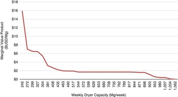
Dryer capacity reaches its maximum seven out of the thirteen weeks of harvest (week 35, 37, 38, 40, 41, 42, 43). Referencing the shadow prices, there are considerable gains to be made by expanding dryer capacity. During week 35, if the dryer capacity could dry 0.03 more MT, it would increase net returns by US$0.79. A similar situation occurs in weeks 37, 40, and 41, but at lower shadow prices of US$0.38, US$0.63, and US$0.70, respectively. Of course, increasing the actual size of the dryer would not take place in the short run, but capacity could be expanded by increasing the temperature at which the dryer runs. However, it is known that this could cause quality issues (shatter) and devalue specifically the specialty grains. Conversely, storage never reaches its full capacity, and no additions can be made to net returns by increasing capacity under the proposed system. A short analysis of the marginal value product (MVP) of weekly dryer capacity was performed and can be referenced in figure 1. As weekly capacity is increased, the value it adds to net returns diminishes per Mg. One constraint that was not emphasized at the beginning of this study, but presents an interesting shadow price, is land. If one more hectare of land were added to the system, net returns would increase by US$745.40, which is much higher than a typical US$432.00/ha rental rate in western Kentucky.
MVP of weekly dryer capacity

Conclusions
Overall, producers with access to variable maturity group planting technology need to be aware of the implications their planting strategy has on net returns and the use of harvest equipment such as dryers and grain bins. As it was shown in the shadow prices associated with the model, if only one of these reaches its full capacity, it can have a significant impact on net returns. This demand for storage and drying equipment is driven by what maturity group was planted when. If a farmer grows a specialty grain such as white corn to increase profitability, the system can become even more constrained. Principally, the model constructed for this paper is an example of the ever-changing and more complex management decisions producers are faced with in the era of precision agriculture. With proper analytical tools, farmers can be better equipped to understand what effect certain technologies have on their production system as a whole. Once they gain this understanding, more profitable decisions can be made and implemented.