2. The model-year 2012–16 light-duty greenhouse gas and fuel economy rules

For light-duty vehicles, NHTSA regulates Corporate Average Fuel Economy (CAFE), expressed in miles per gallon, while EPA has authority over GHGs and regulates grams of carbon dioxide per mile (g/mi). Because the primary way of reducing GHG emissions from vehicles is to reduce fuel consumption, EPA and NHTSA worked closely together as they developed standards to achieve these two goals. While different legal authorities led to the agencies each writing separate sets of standards under their respective statutes, the joint rulemaking produced harmonized standards so that automakers could build one fleet of vehicles across the United States that satisfy all federal and state requirements.Footnote ⁴ As mentioned above, this paper focuses on EPA’s standards and its regulatory analysis; because of minor differences in the programs, the NHTSA calculations are similar but not identical.

Under the rule, by 2016, passenger cars and trucks are projected to achieve a fleet average GHG emission standard of 250 g/mi, equivalent to a CAFE standard of 35.5 mpg if all the emission reductions come from fuel economy.Footnote ⁵ The target fuel economy/GHG level for any individual vehicle, however, depends on its footprint, or the area between a vehicle’s wheels. Larger vehicles are targeted to achieve looser standards than smaller vehicles. The intent of allowing larger vehicles to face a looser standard was to reduce the incentive for vehicle manufacturers to meet the standards in part by producing smaller vehicles.Footnote ⁶ $\!^{,}$ Footnote ⁷ Compliance is based on sales-weighted averaged results for each manufacturer. For instance, a fleet may comply with the standards through large vehicles that exceed their targets and small vehicles that are below their targets.

3. BCA at EPA

Under Executive Orders 12866 and 13563, federal agencies are required to conduct benefit-cost analyses (BCAs) of “significant” rules, including those expected to have impacts of over $100 million per year on the economy. The light-duty GHG/fuel economy standards easily fell into the “significant” category with estimated lifetime costs for MY 2012–16 vehicles of $52 billion (U.S. EPA and DOT, 2010a , p. 25346).

EPA conducts its BCA under the guidance of Circular A-4 (White House, 2003) and its internal Guidelines for Preparing Economic Analyses (U.S. EPA, 2010c ). The principles in these documents reflect standard practices for BCA: identifying the impacts, both positive and negative, intended and ancillary, of a proposed policy, compared to a baseline representing the absence of the policy. These and other guidelines also specify some of the parameters to be used in the analysis. For instance, Circular A-4 specifies the use of 3% and 7% discount rates; the Guidelines provide a value for mortality risk reduction of $7.4 million per statistical life (2006 dollars); and interagency technical support outlines the values to be used for the social cost of carbon (Interagency Working Group on Social Cost of Carbon, 2010). These documents promote consistency in methods and values.

Of course, any particular regulation will have parameters particular to it. For the light-duty vehicle GHG rules, NHTSA and EPA documented most of the parameters used in the BCA in a joint Technical Support Document (TSD; U.S. EPA and DOT, 2010b ). These included the technology cost and effectiveness estimates, the baseline and projected vehicle fleets, average driving amounts, and a number of economic parameters, such as the “rebound rate” (the increase in vehicle miles driven in response to a decrease in the cost of driving due to improved fuel economy) and the impacts of the standards on energy security. The values for these analyses came from a variety of sources, including technical reports, published literature, and internally conducted analyses, cited in the TSD.

There is uncertainty regarding the “true” value of these parameters. In some cases, such as the discount rate and the social cost of carbon, the benefits and costs were calculated several times using alternate parameter values. These calculations allow for the sensitivity of the results across a range of values to be checked. For other parameters, only one value was used for the primary analysis, with side sensitivity analyses. Additional evidence regarding those values would either improve the BCA (if the parameter estimate changes meaningfully) or increase the confidence in the results that are obtained (if the parameter estimates are essentially confirmed). Because the value of the fuel savings were found to be substantially higher than the technology costs, in order for the finding of positive net benefits to be reversed, changes in parameters would have to result in a substantial change in the private costs and benefits of the rule.

Table 1

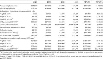
Benefits and costs of EPA’s light-duty greenhouse gas rule, 2010, millions of 2007$.

* SCC refers to the social cost of carbon, the benefit associated with reducing GHG levels; four different estimates of the SCC were used in the assessment, consistent with the Interagency Working Group on Social Cost of Carbon (2010).

Source: EPA and DOT (2010a ), Tables III.H.10-1 through III.H.10-3, pp. 25535–6. Descriptions of all the benefit and cost categories are included in EPA and DOT (2010a ).

4. The light-duty vehicle greenhouse gas BCA and the energy paradox

Table 1 shows EPA’s net benefits calculation for its rule using discount rates of both 3% and 7% and multiple estimates for the social cost of carbon. As seen in the table, the BCA took into account the effect on climate change and energy security, as well as the health effects of other pollutants such as nitrogen oxides and particulate matter, time saved through less need to refuel, and both benefits and costs associated with increased driving due to cheaper costs of driving (the rebound effect). The greatest benefits, however, were expected to come from fuel savings. With the fuel savings benefits per vehicle estimated at approximately $400 per year and additional one-time costs estimated at $950 for MY 2016 vehicles, the payback period to an average consumer for greater fuel efficiency was under 3 years (U.S. EPA, 2010a). Indeed, EPA estimated that an average driver who bought a vehicle on credit could save more in fuel, starting in the first month, than the increase in the loan payment; this result rests on assumptions about technology costs, how the additional costs are passed through to consumers in the final price, car loan rates for the average consumer and the expected amount of driving.Footnote ⁸

If vehicle buyers minimize costs of ownership, as in standard economic models, then all else equal, they should be willing to purchase additional fuel-saving technology as long as the additional cost of this technology to them is less than the expected discounted fuel savings. Given the predicted short payback period, is the failure of the market to provide these estimated fuel savings prima facie evidence that the EPA analysis is missing some costs or overstating benefits? Or, alternatively, does this imply that the market for fuel economy is not resulting in all cost-effective technologies being adopted?

This result is in line with other work that identifies a variety of energy conservation measures, such as building insulation or more efficient light bulbs, that appear to have positive net consumer benefits but are not widely adopted; this phenomenon is commonly termed the “energy efficiency gap” or “energy efficiency paradox” (e.g., Helfand & Wolverton, Reference Helfand and Wolverton2011; Allcott & Greenstone, Reference Allcott and Greenstone2012; Gillingham & Palmer, Reference Gillingham and Palmer2013). An example in the context of fuel economy would be switching from a 4-speed to a 6-speed automatic transmission; this was estimated to cost $99 and reduce GHG emissions/fuel consumption by 4.5%–6.5% (U.S. EPA and DOT, 2010b , Tables 3–32 and 3–37). If a person spends $1500–$2200 on fuel in a year, the fuel savings from using that transmission would recover the initial costs in about a year.Footnote ⁹ If this is correct, it is a puzzle that it has not been in widespread use in vehicles.

A number of hypotheses have been raised for why this efficiency gap could appear (e.g., Helfand & Wolverton, Reference Helfand and Wolverton2011). On the demand side, some potential hypotheses include:

• ∙ High consumer discount rates. If consumers discount future fuel savings at a rate higher than the rates used by the EPA during their estimation of future fuel savings, they will not find the fuel savings as beneficial as the EPA’s calculation suggests and eventually would find that the private costs outweigh the benefits.Footnote ¹⁰ However, while high discount rates may be a straightforward way to model the effects of myopic behavior this does not explain why consumers are myopic.Footnote ¹¹

• ∙ Hierarchical or lexicographic decision-making (e.g., Sallee, Reference Sallee2012). Consumers may limit themselves to vehicles meeting a few characteristics (e.g., body type or price range) instead of evaluating across all vehicle attributes. If manufacturers believe that fuel economy is low in the decision hierarchy, consumers may not have the opportunity to reveal their true preferences for fuel economy. For example, if a buyer had decided on an MY 2010 6-cylinder minivan, she would then face a range of fuel economy of 18–20 mpg, according to fueleconomy.gov. Even if she would have been willing to pay for more fuel economy, the decision to select a minivan foreclosed that option.

• ∙ Consumer difficulty in calculating expected fuel savings. Turrentine and Kurani (Reference Turrentine and Kurani2007) present the results of a survey indicating that many households were either unable to answer, appeared to guess at, or made basic errors in calculating gasoline savings over time for a given improvement in fuel efficiency. Many vehicle buyers may not identify, much less choose, cost-minimizing levels of fuel economy.Footnote ¹²

• ∙ Uncertain future fuel savings contrasted with certain immediate increased costs (Greene, Reference Greene2011). Under prospect theory with a reference point of a given vehicle, loss-averse customers may find the immediate utility loss from the increased cost for a more fuel-efficient vehicle outweighs the gamble associated with an uncertain level of future fuel savings.Footnote ¹³

• ∙ Consumer heterogeneity (Bento, Li & Roth, Reference Bento, Li and Roth2012). While the proposed fuel efficiency improvements are estimated to be cost-effective for the average consumer, there is likely a subset of consumers, perhaps those with low annual miles driven or high discount values, for which the technology is in fact not cost-effective. In this case, the apparent gap may be due in part to people choosing vehicles that are cost-effective for their individual purposes.

Less commonly discussed are possible factors that might generate the efficiency gap, if it exists, from the supply side (Helfand & Wolverton, Reference Helfand and Wolverton2011; U.S. EPA and DOT, 2012; Blumstein & Taylor, Reference Blumstein and Taylor2013).

• ∙ Vehicle manufacturers may believe most consumers are not willing to pay much for some cost-effective improvements to fuel economy and so these are not provided. Similarly, manufacturers might believe that technology that would be cost-effective for the average consumer will not be cost-effective for enough of their customers to use it.

• ∙ Vehicle manufacturers may themselves be risk averse, either in terms of uncertainty in consumer willingness to pay for fuel-saving technologies or in the costs or effectiveness of the new technologies.

• ∙ Vehicle manufacturers may not be able to adjust quickly to changes in consumer demand due to changes in expected fuel prices, so fuel-saving technologies that become cost-effective are not immediately implemented.

• ∙ Market discipline, both through bankruptcy and liquidation at the firm level as well as negative career consequences for executives, may not be sufficiently strong to prevent or quickly correct behaviors that do not maximize profits.

This paper does not take a stand on or provide evidence for which, if any, of the above possible sources of the energy gap are true. Instead, while these possibilities do not necessarily signal market failures, they do suggest ways in which the efficiency gap, where efficient fuel-saving technologies are not fully utilized, could arise.

Allcott and Greenstone (Reference Allcott and Greenstone2012) summarize evidence suggesting that in a number of contexts the energy efficiency gap is substantially smaller than what is found using engineering estimates. While the bases for EPA’s estimates of the technology cost and effectiveness, included in the TSD associated with the rule, were in many cases peer-reviewed, it is possible that EPA’s estimates of the technology costs and effectiveness may have flaws and be too low or too high.

5. The baseline for analysis

Developing a baseline for analysis requires an assessment of what the world would look like in the absence of the proposed policies. EPA’s baseline vehicle fleet started with the MY 2008 vehicle fleet, the most recent one fully available at the time (U.S. EPA and DOT, 2010b , Chapter 1), for sales of individual models and for the technologies that affect fuel use.Footnote ¹⁴ Total sales of cars and light trucks for future years came from projections of the Energy Information Administration (EIA), augmented with market segment data from private sources; these projections were used to estimate future sales volumes for the models in the MY 2008 fleet. This procedure held constant the features of the MY 2008 vehicles, and it did not account for vehicles being dropped from or entering the fleet in future years. The one exception to holding features constant was modeling the addition of technologies to the vehicles so that they would achieve the MY 2011 fuel economy standards already enacted.

Of course, the models offered in MYs 2012–16 in the absence of the standards would not be the same as those in MY 2008. If EPA used a baseline that did not match the future fleet, the analysis might misestimate both costs and benefits associated with the standards. For instance, if automakers would have built more fuel-efficient vehicles in the absence of the standards, then the standards would have less effect on the auto market than projected, and both the costs and the benefits of the standards would be overstated. In addition, if vehicle characteristics such as horsepower would have changed in the absence of the standards, then the technologies estimated to achieve the standards, and thus the cost estimates, might need to be revised. A baseline should project those characteristics into the future, and impacts of the standards would be based on the difference created from that baseline (Klier & Linn, Reference Klier and Linn2013). EPA, however, did not make a projection of changed characteristics. There was no publicly available information about trends in vehicle plans to inform the decisions. The rationale for this approach covered two issues: first, how fuel economy might change in the absence of the standards; and, second, how to address changes in other vehicle characteristics in the absence of the standards.

The expectation that vehicles would not become more fuel-efficient in the absence of the standards was based on history: in years when gas prices and fuel economy standards were stable (e.g., 1986–2003), any overcompliance with the standards was due almost entirely to Japanese manufacturers that produced smaller, lighter vehicles; full-line manufacturers rarely overcomplied (U.S. EPA and DOT 2012, p. 62843).Footnote ¹⁵ In the absence of fuel price shocks, then, the evidence suggested that full-line auto manufacturers, such as the U.S. auto companies, would fashion their fleets to just comply with fuel economy standards. EIA was projecting essentially stable fuel prices into the future. In the absence of sustained increases in vehicle prices, EPA did not find a reason to expect increasing fuel economy in the absence of the standards. Because some cost-effective fuel-saving technologies (e.g., 6-speed automatic transmissions) existed but were not in common use during this era, there did not seem to be a basis to expect their adoption in the absence of the standards.

In contrast, history does not show stability in vehicles’ horsepower (Knittel, Reference Knittel2012); it has increased, except at the time of the initial fuel economy standards.Footnote ¹⁶ Power is generally considered an attribute of which consumers want more; in the absence of the standards, it might continue its trend.Footnote ¹⁷ Power is also considered a substitute for fuel economy (e.g., Klier & Linn, Reference Klier and Linn2012), though it is possible to increase both power and fuel economy, at a cost. One possible approach would be to draw trend lines for horsepower, estimate the vehicle technologies that would be used to achieve those, and add fuel-saving technologies to vehicles with those characteristics.Footnote ¹⁸ Such an effort was considered beyond the information, cost, and time resources available to the agencies. It should be noted that the technology analysis only incorporated known technologies; it is possible that innovations may identify alternative paths to meet the standards, presumably at less cost. An improved baseline estimate that included credible estimated changes in vehicle characteristics could allow for an improved before/after comparison. Klier and Linn (Reference Klier and Linn2013) argue that accounting for these changes in vehicle characteristics may have a substantial effect on consumer welfare.

The fact that it is possible, for a cost, to add both fuel economy and power to a vehicle allows for an alternative way to consider the missing costs associated with not having more power in the projected baseline vehicles. For any future vehicle that would have been built in the absence of the standards, there would be ways to improve the fuel economy. EPA’s cost estimates were based on adding known technology to MY 2008 vehicles. If the same methods to improve fuel economy for that hypothetical future vehicle would have been used for the MY 2008 vehicle, then there would be no opportunity costs unaccounted for in the baseline. If, on the other hand, the greater power of the future vehicle would make it more expensive to improve the fuel economy, then there is a missing cost: the additional expense associated with adding fuel-saving technology to a more powerful vehicle. This value could exist, but EPA did not have ways to estimate it.

Mathematically, if the cost of a vehicle with fuel economy $F$ and power $P$ is $C(F,P)$ , then a Taylor-series expansion suggests that a change in costs can be approximated by:

$$\begin{eqnarray}\text{d}C\approx (\partial C/\partial F)\ast \text{d}F+(\partial C/\partial P)\ast \text{d}P.\end{eqnarray}$$

For a change in fuel economy, then,

$$\begin{eqnarray}\text{d}C/\text{d}F\approx \partial C/\partial F+(\partial ^{2}C/\partial P\partial F)\ast \text{d}P.\end{eqnarray}$$

The first term on the right side is the cost estimate that EPA developed. The missing cost associated with a change in fuel economy, then, is the second term. Even with projections of the change in power, $\text{d}P$ , the cross-partial term is likely to vary with the baseline level of power and the specific technologies used to achieve it. For future BCAs, if credible projections of future characteristics of the vehicle fleet were available, this could be incorporated into the analysis.

Furthermore, the actual attributes of the future vehicle fleet that would have occurred in the absence of the rule (and would ideally be used as a baseline in the BCA) would depend in part on advances in technology. Credible estimates here as well could be beneficial, though perhaps difficult to obtain. It is reasonable to assume, though, that any adopted advances in technology would lower, rather than increase, cost estimates, though the effects on the cross-partial term are harder to predict. EPA’s estimates, if reasonable for known technologies, were thus argued to identify a feasible path to achieving the standards, even if they do not identify the actual strategy that any given firm might use.

6. Measuring benefits under the energy gap

As discussed above, the primary way to reduce GHG emissions from vehicles is to reduce their fuel consumption. The impacts of reduced fuel consumption thus needed to be included in the BCA. Indeed, OMB Circular A-4 explicitly mentions this possibility:

Thus, the official guidance on BCA requires inclusion of averted costs in the BCA.Footnote ¹⁹

For the BCA of the rule, EPA thus needed to find a measure of private benefits that would result from the expected increase in fuel economy. One approach would be to use the preference for fuel economy revealed in the market for vehicles. Another would be to use the estimated discounted fuel savings resulting from the rulemaking. In the absence of an energy efficiency gap, these two values should be the same; here, however, the EPA found different values. The EPA then had to determine which measure of the benefits of increased fuel economy to use.

The literature on BCA in a behavioral context (Gillingham & Palmer, Reference Gillingham and Palmer2013) examines the dilemma over how to respect consumers’ choices when those choices might not reflect their ex post best interests. This literature commonly distinguishes between decision utility, the utility that reflects preferences at the time of a choice, and experienced or true utility, the utility someone experiences after the decision is made (e.g., Kahneman and Sugden (Reference Kahneman and Sugden2005); Beshears, Choi, Laibson and Madrian (Reference Beshears, Choi, Laibson and Madrian2008) and Carlsson (Reference Carlsson2010) refer to this as revealed and normative preferences).

Some authors seek to find ways to bridge the gap between decision and experienced utility. Bernheim and Rangel (Reference Bernheim and Rangel2009), for instance, seek to model preferences in ways that incorporate behavioral economics but nevertheless emphasize the primacy of individuals’ choices (decision utility) as revealing preferences. Smith and Moore (Reference Smith and Moore2010) suggest testing if nonstandard behavior is the result of unmodeled constraints which could then be incorporated. Thaler and Sunstein (Reference Thaler and Sunstein2009) suggest “nudging” choices in what they consider to be noncontroversial directions, as a way to make decision utility better reflect experienced utility. Sugden (Reference Sugden2005) argues that the value employed in a BCA should be one that best represents a market interaction, where market price is a means to bring the two forms of utility closer. Gillingham and Palmer (Reference Gillingham and Palmer2013) suggest that this literature “holds promise, but it is far from ready to be implemented by policymakers.”

Other authors suggest limits on the role of BCA when decision and experienced utility differ. Beshears et al. (Reference Beshears, Choi, Laibson and Madrian2008) recommend that government provide expert advice to individuals when the normative (experienced) recommendation is clear, but then let people choose as they wish. Robinson and Hammitt (Reference Robinson and Hammitt2011), who pursue practical ways to include behavioral insights into BCA, nevertheless conclude by suggesting a constrained use of BCA in policy, as a way of organizing both quantitative and qualitative information, of identifying opportunity costs, and as but one input into a policy decision.

In some cases, such as option or existence value, it may not be clear how to measure experienced utility. For instance, Carlsson (Reference Carlsson2010) notes that stated preference surveys identify revealed (i.e., decision) preferences. In contrast, the new standards present an opportunity to examine decision and experienced utility in a context where, relatively speaking, data exist to measure both decision and experienced utility. For a measure of experienced utility, EPA estimated the change in fuel consumption associated with improving the fuel economy of vehicles, taking into account the additional mileage expected as a result of reducing the cost per mile (U.S. EPA and DOT, 2010a ). This value was multiplied by the predicted fuel prices in the EIA’s Annual Energy Outlook to find the estimated fuel savings. Obtaining relatively credible estimates of benefits apart from willingness to pay may be more difficult when estimating benefits where the main effect of the attribute under consideration involves nonmarketed impacts.

Gayer and Viscusi (Reference Gayer and Viscusi2013) write that the EPA did not have sufficient evidence of inefficiencies in the market for fuel economy to justify using their estimated value of fuel savings instead of consumer willingness to pay as the measure of benefit consumers get from higher fuel economy.Footnote ²⁰ They do allow that inefficiencies in the market for fuel economy are possible, but believe that the evidence presented by EPA for substantial inefficiencies is not great enough to justify not using willingness to pay. In essence, they argue that markets should be assumed to be operating efficiently until they are proven to be otherwise, and thus argue for a decision utility metric.

For decision utility, a number of econometric studies have estimated the willingness to pay for fuel economy as part of the vehicle purchase decision. Empirical studies of the hedonic value of fuel economy in vehicle purchases have found wide variation in results, with about half the studies finding that consumer willingness to pay was less than expected future fuel savings, and about half showing either “correct” valuation or overvaluation (Greene, Reference Greene2010). Two recent papers (Busse, Knittel & Zettelmeyer, Reference Busse, Knittel and Zettelmeyer2013; Sallee, West & Fan, Reference Sallee, West and Fan2011) that focus specifically on the role of fuel economy in vehicle purchase decisions find that the willingness to pay for additional fuel economy approximately equals the expected fuel savings; a third recent paper (Allcott & Wozny, Reference Allcott and Wozny2010), in contrast, continues to findundervaluation.

Fischer, Harrington and Parry (Reference Fischer, Harrington and Parry2007) modeled the value of fuel economy regulation as its actual effect on fuel expenditures (experienced utility), as opposed to how consumers considered its effect at the time of vehicle purchase. As they note, one implication of this approach is that, if the “true value” of fuel economy differs from what consumers are willing to pay at the time of vehicle purchase, then it is possible for fuel economy regulation to make consumers better off than in a baseline scenario with the absence of regulation.

For the BCA of the vehicle GHG standards, EPA, like Fischer et al., relied on the experienced utility measure, rather than the decision utility approach advocated by Gayer and Viscusi. It argued that the experienced utility estimates the expected actual impacts of the rule on fuel consumption, rather than the impacts that consumers considered at the time of vehicle purchase. Regarding decision utility, EPA noted that vehicle buyers may not estimate these impacts accurately and are under no obligation to consider those impacts. Nevertheless, after the vehicle’s purchase, they are expected to receive those fuel savings over its lifetime. To the extent that regulatory analysis is intended to estimate the expected impacts of the rule, the experienced utility measure is aligned with the expected outcomes of the rule. Furthermore, if the recent papers finding that consumers do value fuel economy at approximately the level of the expected fuel savings (Busse et al., Reference Busse, Knittel and Zettelmeyer2013; Sallee et al., Reference Sallee, West and Fan2011) are correct, then measuring benefits through either decision or experienced utility should yield roughly the same result.

Using professional assessments of estimated future benefits in place of people’s perceptions for BCA is also done in other contexts. In BCA of mortality risk, for instance, evidence suggests that people respond to risks based on feelings as well as analysis (e.g. Slovic, Finucane, Peters & MacGregor, Reference Slovic, Finucane, Peters and MacGregor2004). The calculations of risk-related benefits for BCA are nevertheless commonly based on professional calculation of the expected probabilities of adverse outcomes rather than people’s perceptions of those probabilities (e.g., U.S. EPA, 2010c , Chapter 7).

While the EPA used experienced utility to measure the private benefits of the rule, a way to incorporate decision utility in the impacts of the rule would be to include the effects of the rule on vehicle sales. Peoples’ ex ante attitudes influence their vehicle purchase decisions. Incorporating into the BCA the effects of the rule on vehicle sales would account for consumers’ responses to the new vehicles. In practice, though, these impacts were not included, because of the uncertainty associated with consumer response to more expensive but fuel-saving vehicles, with the methods and implications as discussed in Part 5.

7. Estimates of technology costs and compensating variation

Cost and effectiveness measures for various efficiency-improving technologies came from detailed engineering analyses, including tear-down studies that estimated, at the level literally of nuts and bolts, the change in costs for the fuel-saving technologies (e.g., FEV, Inc., 2009). EPA then used its Optimization Model for reducing Emissions of Greenhouse gases from Automobiles (OMEGA) (EPA, 2010b , Chapter 4) to estimate cost-effective ways of achieving specified GHG standards.

Note that EPA’s regulatory analysis sought to identify a feasible path for attaining the standards, not necessarily the path that automakers and consumers would ultimately adopt. An important aspect of these technology cost estimates is that they sought to include the costs of maintaining constant other vehicle attributes. As discussed in Section 5, improvements in fuel economy have been considered substitutes for vehicle power or weight, as improvements in vehicle efficiency could be used for more power, weight, or fuel economy. The analysis underlying the standards argues that this association is not a requirement: for enough money, to a certain extent it is possible to have the same or more power as well as more fuel economy. For instance, changing from an 8-cylinder engine to a smaller displacement 6-cylinder engine generally saves fuel but reduces power. To maintain power, the technology costs for engine downsizing include the addition of turbocharging, which restores the power.Footnote ²¹

For some technologies, it is unclear whether vehicle buyers will consider the new technologies to have the equivalent utility. For instance, stop–start technology turns off the engine when the vehicle is stopped and restarts it as soon as the brake is released. Though the analysis assumed that this technology would not affect vehicle quality, it is possible that some vehicle owners may feel that this technology imposes a cost on them. In the rulemaking process, EPA requested comments on hidden costs associated with the new technologies but did not receive any.Footnote ²² To the extent that the estimates did not capture all relevant outcome characteristics, the cost estimates could be incomplete.

It should also be noted again that the analysis relied on a baseline fleet of vehicles from MY 2008, the most recent available at the time, and held constant the vehicle characteristics for that MY. As discussed earlier, to the extent that the “no-change” baseline is not correct, this may affect the accuracy of the EPA’s estimates of costs. If credible forecasted baselines are available, future BCAs could benefit from their use.

An additional justification for this procedure is that, as noted above, the analysis sought to identify a feasible path for attaining the standards, not necessarily the path that automakers and consumers would ultimately adopt. This approach had the practical implication that changes to vehicle and fleet attributes, apart from fuel economy and levels of GHG emissions, as a result of the rule would be adopted only if they were expected to increase welfare above the outcome where these characteristics did not change in response to the rule. Because of this approach, the net costs of consumer gains from a different path must be less than the technology costs of the baseline fleet. This argument can be demonstrated based on compensating variation, as outlined here.

Let the utility of consumer $i$ be dependent on a measure of the quality of the vehicle purchased and an outside good:

(1) $$\begin{eqnarray}\mathit{Utility}_{i}=U(\mathit{VehicleQuality}_{i},\mathit{OutsideGood}_{i}).\end{eqnarray}$$

The consumer faces the budget constraint

(2) $$\begin{eqnarray}\mathit{Wealth}_{i}=\mathit{VehicleCost}_{i}+\mathit{OutsideGoodExpenditure}_{i}\end{eqnarray}$$

where $\mathit{VehicleQuality}_{i}$ is a measure of the utility that vehicle owner $i$ receives from the vehicle, measuring attributes such as size, power, or comfort in such a way that an additional dollar expended on quality leads to a constant increase in the perceived quality. (The analysis easily generalizes if vehicle quality is measured with a vector of attributes instead of a single-dimensioned vehicle quality measure, or if the technology costs to comply with the rule vary with vehicle quality, as long as they vary monotonically.) VehicleCost, the cost to the vehicle buyer, is a function of vehicle quality, where, as above, the cost per unit for additional vehicle quality is constant. Utility is increasing in both VehicleQuality and OutsideGood. Note that because fuel economy and fuel savings were accounted for in the benefits discussion above and this section focuses on costs, fuel economy is not taken into account in the measure of vehicle quality, and fuel costs are ignored in the budget constraint.Footnote ²³

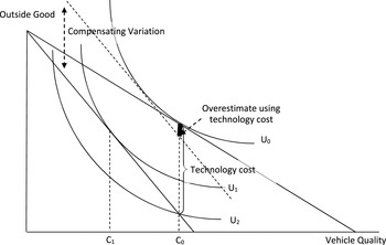
Figure 1 shows the initial vehicle selection for a representative consumer, with vehicle quality $C_{0}$ and utility $U_{0}$ . Assume the standards increase the marginal cost of vehicle quality from $p_{0}$ to $p_{1}$ , by requiring additional fuel-saving technology, so that the budget constraint shifts inward.

The additional cost to purchase the same vehicle after the price change is the vehicle’s technology cost if increases in production costs are fully passed through from the manufacturers to the consumer.Footnote ²⁴ Thus the technology cost can also be seen as the amount of money that the consumer needs to be compensated in order to remain at her original utility level, $U_{0}$ , while purchasing the original vehicle quality, $C_{0}$ , under the higher prices. If $e(p,U)$ is the minimum expenditure necessary to receive utility $U$ when prices are $p$ , then the technology cost can be written as:

(3) $$\begin{eqnarray}\mathit{TechCost}=e(p_{1},U_{0}\mid \mathit{VehicleQuality}=C_{0})-\mathit{Wealth}\end{eqnarray}$$

In Figure 1, this choice corresponds to the point where $C_{0}$ is on the new budget constraint.

A consumer is unlikely to stay with quality $C_{0}$ , though; in Figure 1, a utility-maximizing consumer will switch to bundle $C_{1}$ , with lower vehicle quality, to have more of the outside good. The compensating variation labeled on Figure 1 is the amount of additional money that the consumer needs in addition to her original wealth to return to the original utility level $U_{0}$ after the price of vehicle quality increased to $p_{1}$ .Footnote ²⁵ The compensating variation can be written as:

(4) $$\begin{eqnarray}CV=e(p_{1},U_{0})-\mathit{Wealth}\end{eqnarray}$$

with $\mathit{Wealth}=e(p_{0},U_{0})$ .

Figure 1

Comparison of technology cost and compensating variation.

As shown in Figure 1, because the dotted line corresponding to $e(p_{1},U_{0})$ lies below the original budget constraint at quality $C_{0}$ , the compensating variation is smaller than the technology cost of complying with the rule. This is because, according to the law of compensated demand, the least expensive way to achieve the original utility under higher prices for vehicle quality involves purchasing less vehicle quality. The financial compensation necessary for the consumer to reach her original utility under the higher prices is smaller if she reduces the amount of vehicle quality purchased (CV) than if she does not (technology cost). This also implies that, if the private benefits to the consumer meet or exceed the technology costs, then they also meet or exceed the compensating variation. Thus, as long as EPA estimated the full technology costs with reasonable accuracy and the no-change baseline is correct, those costs fully account for costs to consumers. Future BCAs taking an engineering approach to estimating costs could use similar arguments to avoid the difficulties of projecting changes in outcomes as a result of proposed actions. This argument, however, does not assist in determining an appropriate baseline outcome in the absence of the rule.