





Introduction
Radar has evolved into a reliable and omnipresent technology for ranging, detection, and localization applications. Typically, in such applications, the radar target is far away from the radar system, which aims to determine the target’s position and velocity. However, radar technology is increasingly used for short-range sensing applications as well. On the one hand, the low-cost availability of integrated radar transceivers makes radar technology applicable for sensing tasks for widespread customer mass products. On the other hand, radar-based sensing drives research activities for new applications. These include hand gesture recognition [Reference Bräunig, Wirth, Kammel, Schüßler, Ullmann, Stamminger and Vossiek1, Reference Stadelmayer, Santra, Weigel and Lurz2], material characterization [Reference Barowski, Zimmermanns and Rolfes3], biomedical imaging [Reference Klemm, Leendertz, Gibbins, Craddock, Preece and Benjamin4], smoke detection [Reference Schenkel, Schultze, Baer, Balzer, Rolfes and Schulz5], as well as vital-sign sensing, including heart sound detection [Reference Wenzel, Albrecht, Langer, Heyder and Koelpin6, Reference Albrecht, Heyer, Wenzel, Langer, Lu and Koelpin7]. In contrast to traditional applications, the radar sensors then often operate at close ranges to the target, where the range becomes comparable to the target dimension. With the trend toward higher operating frequencies in the millimeter-wave bands, this implies the onset of near-field wave propagation effects, which conventionally are disregarded, but may be critical for reliable performance [Reference Tegowski, Langer, Albrecht and Koelpin8].
The concept of the radiative near-field and far-field regions is well-known for antennas, which follows from the antenna aperture size [9, Reference Balanis10]. Analogously, the differentiation between near field and far field also applies to the scattering from a target. Here, the far-field distance is dictated by the size of the target. Accordingly, once the radar antenna is located at a distance  $z$, which is comparable to the size
 $D$ of an electrically large target, it will be in the target’s radiative near field. One of the consequences is that the incident field illumination, as shown in Figure 1 for the exemplary application of radar-based vital-sign sensing, becomes inhomogeneous and, thus, cannot be approximated by a plane wave, as in target-far-field conditions.
Accordingly, the illumination and, thus, the scattering, become distance-dependent; compare Figure 1(a) with (b). Similarly, the scattering contributions from different regions of the target are individually weighted by the receive antenna according to its spatial selectivity.
Thus, in the target near field, the characterization of scattering on the system level cannot be conducted by a target-inherent radar cross section (RCS) in conjunction with the well-known radar equation. Similarly, the definition of a range-dependent near-field RCS [Reference Pouliguen and Desclos11], which presumes isotropic antennas, provides an incomplete description since, even though it accounts for the spherical nature of wave propagation, it neglects the antenna characteristic. However, as the antenna characteristic weights the incident field illumination in terms of amplitude and phase distribution (see Figure 1), the antenna cannot be decoupled from the analysis of near-field scattering [Reference Tegowski, Langer, Wenzel, Albrecht and Koelpin12, Reference Taylor and Terzuoli13]. As a result, the complete characterization requires a conjunct analysis of the antenna-target system, which is given by the radar channel transfer function [Reference Tegowski, Langer, Albrecht and Koelpin8, Reference Tegowski, Langer, Wenzel, Albrecht and Koelpin12, Reference Tegowski, Langer, Albrecht and Koelpin14] that relates the outward-going power wave ( $\underline{b}$) to the forward-propagating one (
 $\underline{a}$) at the antenna feed port, as visualized in Figure 1.
Near-field scattering scenario. The radar antenna is located in the near field of an electrically large target, whereas the target is in the far field of the antenna. The color gradient on the target surfaces indicates the normalized incident field strength.

Figure 1 Long description
Two diagrams labeled as a and b illustrate radar channel transfer functions. In both diagrams, the radar channel transfer function is represented by the equation R equals b over a. Diagram a shows a radar transceiver on the left, connected to a circular pattern labeled G left parenthesis theta comma phi right parenthesis, indicating the radiation pattern. The pattern is directed towards a human figure on the right, with a color gradient indicating dBmax values ranging from minus 40 to 0. Diagram b similarly depicts the radar channel transfer function with the same equation, but highlights the radiation pattern and incident field directed towards the human figure. The color gradient on the human figure is consistent with the dBmax scale, showing variations in field strength. Both diagrams emphasize the interaction between the radar transceiver and the human figure, illustrating the violation of far-field conditions.
The phenomena that arise in the target near field can be categorized into spatial receive power level fading [Reference Tegowski, Langer, Wenzel, Albrecht and Koelpin12, Reference Tegowski, Langer, Albrecht and Koelpin14, Reference Pouliguen and Desclos15] and nonlinear phase distortions relative to the far-field relationships [Reference Tegowski, Langer, Wenzel, Albrecht and Koelpin12, Reference Tegowski, Langer, Albrecht and Koelpin14]. In addition, because of the short range within the target near field, multiple reflections between the target and the antenna due to the antenna RCS and radar self-RCS may be significant for accurate measurements [Reference Tegowski and Koelpin16, Reference Tegowski and Koelpin17]. However, the associated impairments occur on a smaller scale compared to the power-level fading and nonlinear phase distortion effects, which dictate the overall behavior of the near-field radar channel.
To investigate the impact of the near-field phenomena on the radar receive signal in practical applications, a simulation framework is required that captures the relevant effects. Noting the electrically large size of the targets, a fast simulation with a low computational effort is particularly advantageous. This is key to examine the performance of radar systems for a multitude of configurations. This is relevant in light of the multidimensionality of the radar channel transfer function introduced by the dependence on range and the antenna, which is in contrast to the conventional RCS-based far-field analysis. Thus, computationally expensive full-wave simulations are often not reasonably applicable, and one relies on high-frequency approximation techniques such as geometrical-optics-based ray-tracing [Reference Williams, Tirado, Chen, Gonzalez-Valdes, Martinez and Rappaport18, Reference Ruck19] or physical-optics-based approaches [Reference Tegowski, Langer, Wenzel, Albrecht and Koelpin12, Reference Ruck19, Reference Körner, Altholz, Gerling, Barowski, Schulz and Rolfes20]. The physical optics concept derives from integral solutions of Maxwell’s equations and can be adapted to near-field scattering problems [Reference Tegowski, Langer, Wenzel, Albrecht and Koelpin12, Reference Pouliguen and Desclos15]. It yields closed-form solutions for the radar channel, which enables an analytical examination of the dependencies. Even though the antenna is in the near field of the electrically large target, the target is typically in the far field of the antenna in short-range applications. Given these conditions, the antenna’s behavior can be incorporated by means of its far-field gain and phase patterns. Following this principle, a physical-optics-based monostatic radar channel transfer function that accounts for the spatial selectivity of the antenna is derived in [Reference Tegowski, Langer, Wenzel, Albrecht and Koelpin12] and validated for simple targets [Reference Tegowski, Langer, Wenzel, Albrecht and Koelpin12] as well as complex-shaped objects such as human-body-like shapes in [Reference Tegowski, Langer, Albrecht and Koelpin8, Reference Tegowski, Langer, Albrecht and Koelpin14].
This article extends the contribution presented at the 2025 55th European Microwave Conference and published in its proceedings [Reference Tegowski, Langer, Albrecht and Koelpin14] by providing more details on the simulation framework tailored to evaluate the radar channel transfer function. In particular, absorption effects due to finite conductivity or dielectric losses are incorporated in this article to the simulation approach from [Reference Tegowski, Langer, Albrecht and Koelpin14]. Moreover, this article discusses the required sampling density and convergence of the numerical implementation of the radar channel evaluation.
The article is organized as follows. Section “Theory” reviews the derivation of the radar channel transfer function, including absorption effects. Section “Numerical implementation” discusses the target surface sampling density in conjunction with the convergence. It furthermore provides details on the implementation of the simulation framework. Section “Measurements” presents the experimental validation. Section “Conclusion” summarizes the article.
Theory
This section reviews the derivation of the radar channel transfer function 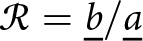 ${\mathcal{R} = \underline{b}/\underline{a}}$, which relates the output power wave phasor
 $\underline{b}$ to the incident one
 $\underline{a}$ at the antenna terminal, as indicated in Figure 1. The derivation relies on the Stratton–Chu integrals [Reference Tegowski, Langer, Wenzel, Albrecht and Koelpin12, Reference Ruck19]. Assuming an
 $\exp(\mathrm{j}\omega t)$ time dependence, the magnetic field at position
 $\mathbf{r}$ scattered by a target is given by [Reference Ruck19]
 \begin{align}\mathbf{H}^S \! (\mathbf{r}) = &\frac{1}{4\pi} \int_S \Bigl\{(\hat{\mathbf{n}} \times \mathbf{H}^{T}) \times \nabla\psi_0 \\ \nonumber&+\mathrm{j}\frac{k}{\eta}(\hat{\mathbf{n}}\times\mathbf{E}^{T})\psi_0 + \langle \hat{\mathbf{n}}, \mathbf{H}^{T} \rangle \nabla \psi_0 \Bigr\} dS .\end{align}
It is determined by the total electric  $\mathbf{E}^{T}$ and magnetic fields
 $\mathbf{H}^{T}$ at the closed scatterer surface
 $S$, where
 $\hat{\mathbf{n}}$ is the outward-pointing unit normal vector at the surface element
 $dS$ located at
 $\mathbf{r}^\prime$. An analogous relationship holds for the scattered electric field [Reference Ruck19]. Boldface letters (
 $\mathbf{a}$) denote vectors, where hat-symbols (
 $\hat{\mathbf{a}}$) indicate unit vectors.
 $\langle \cdot, \cdot \rangle$ denotes the dot product,
 $\lVert \cdot \rVert$ is the Euclidean norm, and
 $\mathrm{j}=\sqrt{-1}$ is the imaginary unit. Moreover,
 \begin{equation}
\psi_0 = \frac{\exp(-\mathrm{j} k \lVert\mathbf{r} - \mathbf{r}^\prime\rVert)}{\lVert\mathbf{r} - \mathbf{r}^\prime\rVert}
\end{equation}
is the Green’s function of free space,  $k$ denotes the wavenumber, and
 $\eta$ is the intrinsic impedance of the environmental medium. In (1), the gradient
 $\nabla$ operates with respect to
 $\mathbf{r}^\prime$.
To approximate the total fields at the scatterer surface  $S$, the tangent-plane approximation is applied in accordance with the physical optics approach. For this, the target shape is restricted to exhibit radii of curvature much larger than the wavelength [Reference Ruck19]. In particular, edges and sharp corners leading to diffraction effects are excluded. Then, the total fields can be approximated by expressing them in terms of the incident fields based on the elementary plane wave reflection at an infinitely extending plane material interface, which is governed by the law of reflection. The electromagnetic properties of a nonmagnetic target material are accounted for by the Fresnel coefficients, which depend on the ratio of the intrinsic impedances [Reference Ruck19, Reference Pozar21]
 \begin{equation}
\eta^\prime = \frac{\eta_\text{Target}}{\eta_0}
\end{equation}
between the target  $\eta_\text{Target}$ and the environmental medium
 $\eta_0 =\sqrt{\mu_0/\varepsilon_0}$, which is assumed to be free space.
 $\varepsilon_0$ and
 $\mu_0$ are the free-space permittivity and permeability, respectively. For lossy dielectrics with a complex-valued relative permittivity
 $\varepsilon_r=\varepsilon_r^\prime - \mathrm{j}\varepsilon_r^{\prime\prime} = \varepsilon_r^\prime[1-\mathrm{j}\tan(\delta)]$, and loss tangent
 $\tan(\delta)$, the intrinsic impedance reads [Reference Pozar21]
 \begin{equation}
\eta_\text{Target} = \sqrt{\frac{\mu_0}{\varepsilon_0\varepsilon_r^\prime [1-\mathrm{j}\tan(\delta)]}},
\end{equation}
whereas for conductors with conductivity  $\sigma$, it holds [Reference Pozar21]
 \begin{equation}
\eta_\text{Target} = \sqrt{\frac{\mathrm{j}\omega\mu_0}{\sigma}}.
\end{equation}
It is assumed that the penetration depth, either due to conductivity or high dielectric losses, is sufficiently small that wave interactions beyond the first material interface are negligible.
To approximate the incident field, one exploits spherical wave propagation together with the gain pattern 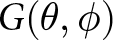 $G(\theta,\phi)$ and phase pattern
 $\Psi(\theta,\phi)$ of the antenna. For this, one presumes that the target is located in the far-field region of the antenna. However, note that the reverse relationship does not require far-field conditions, i.e., the antenna can be located in the near field of the target. Consequently, the field incident on
 $dS$ reads [Reference Tegowski, Langer, Albrecht and Koelpin8, 9]
 \begin{equation}
\mathbf{H}_\text{inc} = {\mathrm{j} \underline{a} \sqrt{\frac{G(\mathbf{r}^{\prime})}{4\pi \eta \lVert\mathbf{r}^{\prime}\rVert^2}} e^{-\mathrm{j}[k\lVert\mathbf{r}^{\prime}\rVert - \Psi(\mathbf{r}^{\prime})]} }\cdot \hat{\mathbf{h}}_\text{inc}
\end{equation}
where the unit vector  $\hat{\mathbf{h}}_\text{inc}$ defines the polarization of the incident magnetic field strength at
 $dS$. Because of the far-field condition, it follows from the unit vectors of a spherical coordinate system
 $(\theta,\phi)$. It is assumed that the position of the antenna defines the origin of the coordinate system. Assuming linear polarization, the polarization vector
 $\hat{\mathbf{h}}_\text{inc}$ makes an angle
 $\nu$ with the normal vector of the plane of incidence defined by
 $\mathbf{r}^\prime\times\hat{\mathbf{n}}$. Following the tangent-plane approximation, the fields at the shadowed subsurface of
 $S$ that is not visible from the perspective of the antenna are set to zero, as indicated in Figure 1.
The contribution from each surface element  $dS$ to the received power wave
 $\underline{b}$ is given by the evaluation of the associated scattered field at the antenna position and weighting it by the antenna effective area and the phase pattern corresponding to the observation direction. Combining all relationships, the radar channel transfer function is derived as [Reference Tegowski, Langer, Albrecht and Koelpin8, Reference Tegowski, Langer, Wenzel, Albrecht and Koelpin12]
 \begin{align}\mathcal{R} = \int_{\bar{S}} {G(\mathbf{r}^{\prime}) e^{2\mathrm{j}\Psi(\mathbf{r}^{\prime})}}& \cdot{\frac{e^{-2\mathrm{j} k\lVert\mathbf{r}^{\prime}\rVert}}{4\pi \lVert\mathbf{r}^{\prime}\rVert^3}} \langle \hat{\mathbf{n}}, \mathbf{r}^\prime \rangle \\ \notag& \cdot \left[ (\Gamma_H + \Gamma_E) \cos^2(\nu) - \Gamma_E \right] d\bar{S}\end{align}
where  $\bar{S}$ denotes the subsurface of
 $S$ visible from the perspective of the antenna. The Fresnel reflection coefficients are given by [Reference Tegowski, Langer, Albrecht and Koelpin8, Reference Ruck19, Reference Pozar21]
 \begin{equation}
\Gamma_E = \frac{\eta^\prime \cos\theta_\text{inc} - \sqrt{1 - {\eta^\prime} ^2 (1-\cos^2\theta_\text{inc})}}{\eta^\prime \cos\theta_\text{inc} + \sqrt{1 - {\eta^\prime} ^2 (1-\cos^2\theta_\text{inc})}}
\end{equation}
and
 \begin{equation}
\Gamma_H = \frac{\cos\theta_\text{inc} - \eta^\prime \sqrt{1 - {\eta^\prime}^2 (1-\cos^2\theta_\text{inc})}}{\cos\theta_\text{inc} + \eta^\prime \sqrt{1 - {\eta^\prime}^2 (1-\cos^2\theta_\text{inc})}}
\end{equation}
where  $\cos(\theta_\text{inc}) = \langle \hat{\mathbf{n}}, \mathbf{r}^\prime \rangle/\lVert\mathbf{r}^\prime\rVert$ with
 $\theta_\text{inc}$ denoting the angle of incidence. For further details on the derivation, the reader is referred to [Reference Tegowski, Langer, Albrecht and Koelpin8, Reference Tegowski, Langer, Wenzel, Albrecht and Koelpin12].
Numerical Implementation
For the numerical evaluation of (7), the target surface needs to be discretized into  $N$ surface elements with individual surface areas
 $dS_i$. Then, the radar channel transfer function is approximated by a finite sum
 \begin{equation}
\mathcal{R}_N = \frac{1}{4\pi}\sum_{i=1}^{N} \mathcal{R}_{N,i} \approx \mathcal{R}
\end{equation}
with the contribution of each surface element
 \begin{align}\mathcal{R}_{N,i} &= G_i e^{2\mathrm{j} \Psi_i} \frac{e^{-2\mathrm{j} k \lVert\mathbf{r}_i^\prime\rVert}}{ \lVert\mathbf{r}_i^\prime\rVert^3} \langle \hat{\mathbf{n}}_i, \mathbf{r}_i^\prime \rangle \\ \notag& \cdot \underbrace{\left[ (\Gamma_{H,i} + \Gamma_{E,i}) \cos^2(\nu_i) - \Gamma_{E,i} \right]}_{= M_i} d\bar{S}_i.\end{align}
The subscript  $i$ denotes that each of the quantities is evaluated for the particular surface element
 $i$. The term
 $M_i$ summarizes the material-dependent factor, which depends on the Fresnel coefficients and the relative polarization angle
 $\nu$.
This section discusses the details of the numerical evaluation of (7). First, the required sampling density is discussed in terms of convergence. Then, the implementation of a simulation framework for practical target shapes is presented.
Convergence
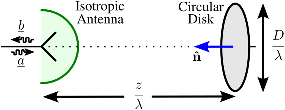
To investigate the impact of sampling density on convergence, the example depicted in Figure 2 is considered.
Exemplary configuration for the convergence analysis consisting of an isotropic antenna and a circular disk as target.

It consists of an isotropic antenna at a distance of  $z/\lambda$ from a circular disk of diameter
 $D/\lambda$.
 $\lambda$ denotes the wavelength. The antenna position intersects with the rotational axis of the disk. The disk is made out of perfect electric conductor (PEC). In this case,
 $M_i=1$ and (10) can be rewritten as
 \begin{align}
\mathcal{R}_N &= \frac{1}{4\pi}\sum_{i=1}^{N} \frac{e^{-2\mathrm{j} k \lVert\mathbf{r}_i^\prime\rVert}}{\lVert\mathbf{r}_i^\prime\rVert^3} \langle \hat{\mathbf{n}}_i, \mathbf{r}_i^\prime \rangle d\bar{S}_i \\ \nonumber
&= \frac{1}{4\pi}\sum_{i=1}^{N} \frac{e^{-4\pi\mathrm{j} \lVert\mathbf{r}_{i,\lambda}^\prime\rVert}}{\lVert\mathbf{r}_{i,\lambda}^\prime\rVert^3} \langle \hat{\mathbf{n}}_i, \mathbf{r}_{i,\lambda}^\prime \rangle d\bar{S}_{i,\lambda} .\end{align}
The problem of convergence can be analyzed in a wavelength-normalized spatial domain since the summands in (12) are invariant with respect to scaling of the entire geometry in proportion of the wavelength  $\lambda$, i.e.,
 $\mathbf{r}_{i,\lambda}^\prime = \mathbf{r}^\prime_i /\lambda$. Accordingly, the number of surface elements
 $N$ controls the convergence based on the normalized area
 $ {d\bar{S}}_{i,\lambda} = {d\bar{S}}_{i}/\lambda^2$ of the surface elements.
To examine the convergence, the disk surface is subdivided into  $N$ surface elements, each associated with a sampling point, where
 $N-1$ of them exhibit an equal area
 $d\bar{S}_\lambda$, while the remaining one in the center completes the total surface area of the disk. The discretization is constructed to uniformly distribute the sampling points along the radial direction while maintaining an equal surface element area of
 $d\bar{S}_\lambda$. The normalized sampling density
 ${\rho_\lambda = 1/d\bar{S}_\lambda}$ is given by the inverse of the normalized surface element area. Figure 3 shows different examples of the discretization.
Examples of different normalized sampling densities  $\rho_\lambda$. The normalized diameter of the disk is
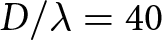 $D/\lambda = 40$.

Figure 3 Long description
A scatter plot of points inside a circle. The title reads, rho subscript lambda equals 0.1. The x-axis label reads, x over lambda, with tick labels at minus 20, minus 10, 0, 10, 20. The y-axis label reads, y over lambda, with tick labels at minus 20, minus 10, 0, 10, 20. Points form a sparse grid across the circular area. The image B showing a scatter plot of points inside a circle. The title reads, rho subscript lambda equals 0.2. The x-axis label reads, x over lambda, with tick labels at minus 20, minus 10, 0, 10, 20. The y-axis label reads, y over lambda, with tick labels at minus 20, minus 10, 0, 10, 20. Points form a denser grid than image A across the circular area. The image C showing a scatter plot of points inside a circle. The title reads, rho subscript lambda equals 0.4. The x-axis label reads, x over lambda, with tick labels at minus 20, minus 10, 0, 10, 20. The y-axis label reads, y over lambda, with tick labels at minus 20, minus 10, 0, 10, 20. Points form a dense grid across the circular area. The image D showing a scatter plot of points inside a circle. The title reads, rho subscript lambda equals 0.8. The x-axis label reads, x over lambda, with tick labels at minus 20, minus 10, 0, 10, 20. The y-axis label reads, y over lambda, with tick labels at minus 20, minus 10, 0, 10, 20. Points form the densest grid among the four images across the circular area.
The convergence is quantified by means of the absolute variation
 \begin{equation}
e_N = | \mathcal{R}_{2N} - \mathcal{R}_{N} |
\end{equation}
between the radar channel transfer function  $\mathcal{R}_{2N}$ evaluated with
 $2N$ sampling points and the transfer function
 $\mathcal{R}_N$ evaluated with
 $N$ sampling points for the exact same configuration. Thus, (13) measures the impact on the radar channel result due to doubling of the sampling density.
Relative convergence versus the normalized sampling density for different parameter sets of the exemplary configuration from Figure 2: normalized distance  $z/\lambda$ = (50, 100, 200) (colors) and normalized diameter
 $D/\lambda$ = (40, 80) (solid, dotted).

Figure 4 Long description
The horizontal axis is labeled, Sampling Density rho subscript A, with tick labels 0.1, 1, 10, 100 and 1000. A second horizontal axis is labeled, Normalized Area dS, with tick labels 10, 1, 0.1, 0.01, 0.001. The vertical axis is labeled, 20 log subscript 10 of e subscript N, with tick labels minus 20, minus 40, minus 60, minus 80, minus 100, minus 120 and minus 140. A legend lists D over lambda equals 40 and 80 and z over lambda equals 50, 100 and 200. Six lines are shown, with three solid lines and three dotted lines. All six lines slope downward from left to right. Near sampling density 0.1, the upper group of lines is around minus 20 to minus 40 and the lower group of lines is around minus 60 to minus 80. Around sampling density 1, the upper group is around minus 40 to minus 60 and the lower group is around minus 80 to minus 100. Around sampling density 10, the upper group is around minus 70 to minus 90 and the lower group is around minus 100 to minus 120. Around sampling density 100, the upper group is around minus 100 to minus 115 and the lower group is around minus 120 to minus 135. Near sampling density 1000, the upper group is around minus 120 to minus 130 and the lower group is around minus 135 to minus 145.
Figure 4 evaluates the convergence  $e_N$ for the exemplary parameter combinations
 $D/\lambda=\{40, 80\}$ and
 $z/\lambda = \{50, 100, 200\}$. The exact convergence depends on the particular configuration. This stems from the
 ${\exp(-4\pi\mathrm{j} \lVert\mathbf{r}_{i,\lambda}^\prime\rVert)}$ contribution in (12), which experiences different variations of the phase term
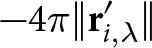 ${-4\pi \lVert\mathbf{r}_{i,\lambda}^\prime\rVert}$ across the sampling points depending on the distance and target dimension. With decreasing distance, the phase change across the disk increases due to spherical wave propagation, thus requiring a finer sampling density. This dependence similarly applies for increasing the disk diameter at a constant distance, which necessitates finer sampling for a particular convergence threshold. The considered exemplary configuration serves as guidance for the sampling density required to reach a particular numerical accuracy. For practical configurations with real-world complex-shaped targets and directive antennas, the necessary sampling density may be subject to change due to the additional weighting of the summands in (12) by the gain pattern as well as the dot product
 $\langle \hat{\mathbf{n}}_i, \mathbf{r}_{i,\lambda}^\prime \rangle$.
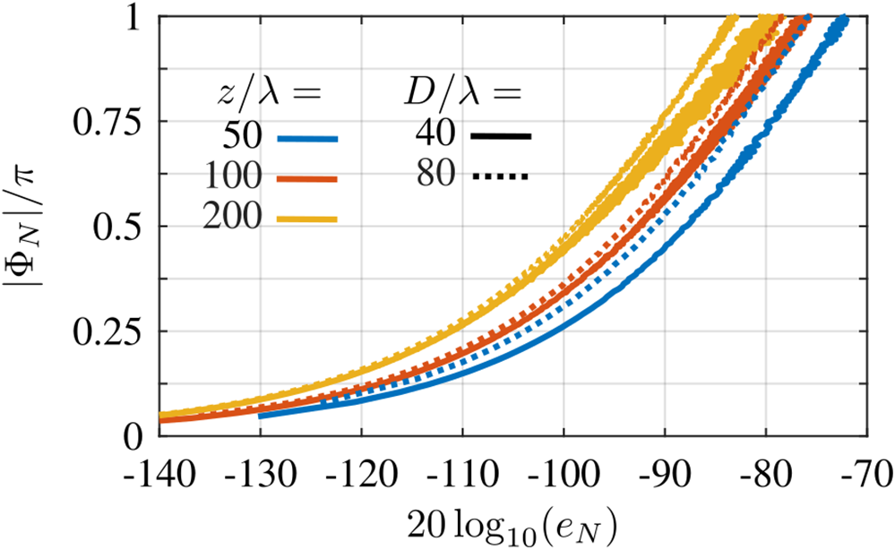
Because (12) is a summation of complex numbers, a sufficient sampling density must be provided to prevent out-of-phase cancellations due to undersampling. If the sampling density is too coarse, the convergence measure  $e_N$ shows varying oscillatory behavior; see Figure 4. Thus, convergence is reached once this density threshold is surpassed. Accordingly, the convergence can be examined by evaluating the maximum phase variation over all sampling points
 \begin{equation}\Phi_N = \max_i \left[ \arg \left( \frac{\mathcal{R}_{N,j}}{\mathcal{R}_{N,i}} \right) \right]
\end{equation}
between the phase at the sampling point  $i$ and the immediately neighboring sampling point
 $j$. Figure 5 evaluates
 $\Phi_N$ as a function of the convergence measure
 $e_N$ for the considered disk target example and the simulated sampling densities.
Maximum phase change  $\Phi_N$ across neighboring evaluation points versus the convergence measure
 $e_N$ for different parameter sets of the exemplary configuration from Figure 2: normalized distance
 $z/\lambda$ = (50, 100, 200) (colors) and normalized diameter
 $D/\lambda$ = (40, 80) (solid, dotted).

Based on the results, the convergence can be estimated given the target distance and its overall dimension from the maximum phase variation between neighboring sampling points. For the considered examples, a convergence below  $-$100 dB results for a maximum phase change of
 ${|\Phi_N| \lt \pi/4}$. This phase difference translates to a maximum equivalent distance between neighboring sampling points of
 $\pi/(4 \cdot 2k) = \lambda/16$ assuming a 90
 $^\circ$ incidence angle as a worst-case estimation. However, as practical configurations are typically dominated by non-grazing incidence, the sampling density can often be significantly reduced without violating the maximum phase variation threshold.
Simulation framework
The evaluation of (7) for practical target shapes is based on the simulation framework visualized in Figures 6 and 7. The vital-sign sensing application configuration shown in Figure 6(a) serves as an example for a complex-shaped target object, which cannot be defined analytically. However, the simulation framework also applies to other target shapes as long as the underlying model assumptions outlined in Section “Theory” are satisfied.
(a) Exemplary view of the simulation framework. (b) Close-up view of the triangle mesh. (c) Definition of the coordinate system.

Figure 6 Long description
Three parts labeled as (a), (b) and (c). In part (a), a human figure is shown with the label ′Target STL File′ on the left and ′Far-Field Antenna Pattern′ on the right. Arrows in various colors represent different directions and components, including u subscript theta, u subscript phi, v and w. Part b is a close-up view of a triangle mesh, showing points labeled a subscript i, b subscript i and c subscript i, connected by lines forming a triangle. Part c illustrates the definition of the coordinate system with axes labeled x, y and z. Arrows in different colors indicate directions and components such as u subscript theta, u subscript phi, v and w, along with angles phi and theta. The diagram visually represents the simulation framework used for evaluating the radar channel transfer function for different target shapes and antenna patterns.
Overview of the simulation framework and the interdependencies between the quantities.

Figure 7 Long description
Two labeled parts are connected by arrows. The part titled, STL-File Target Model shows a triangulated surface with one triangle highlighted and its three vertices labeled a subscript i, b subscript i and c subscript i, with additional vertex markers around the mesh. Beneath it, a bracketed list shows triangle vertex sets written as left brace a subscript 1, b subscript 1, c subscript 1 right brace, left brace a subscript 2, b subscript 2, c subscript 2 right brace, left brace a subscript i, b subscript i, c subscript i right brace and left brace a subscript N, b subscript N, c subscript N right brace. A downward arrow leads to a row of boxed expressions that include n subscript i and r prime subscript i and a box containing T left parenthesis n subscript i comma r prime subscript i right parenthesis. From this row, arrows point to the right toward the part titled, Antenna Far-Field Pattern. That part shows a three dimensional lobe shape with axis labels u and v and an angle label theta. Below it is a square u comma v plane with u marked along the horizontal direction and v marked along the vertical direction and numeric endpoints labeled minus 1 and plus 1 on both axes. Inside the square, text lists G left parenthesis u comma v right parenthesis and psi left parenthesis u comma v right parenthesis. A downward arrow from the u comma v square leads to a row of boxes that includes a box labeled u subscript i comma v subscript i and boxes labeled G subscript i and psi subscript i. Additional boxes in the same row include an expression with cos superscript 2 left parenthesis nu subscript i right parenthesis and a box labeled k. Beneath these, a long horizontal box contains summation notation and ends at a box labeled R subscript N. Along the bottom, two boxed instructions read, for all i colon Evaluate left parenthesis 24 right parenthesis and L colon Evaluate left parenthesis 23 right parenthesis, with arrows pointing upward into the computation boxes and then onward to the final R subscript N.
The simulation framework has two inputs: the target model and the antenna model. The target model is provided by an STL-file, which describes the target surface as a mesh of triangles defined by their vertices  $\{\mathbf{a}_i, \mathbf{b}_i, \mathbf{c}_i\}$, see Figure 6(b). The antenna radiation characteristic is given by the far-field gain pattern and phase pattern of the considered antenna. These can stem from full-wave simulation or be analytically defined. It is assumed that the coordinate system of the antenna, shown in Figure 6(c), defines the global coordinate system, in which the target geometry is described. To change the relative distance and orientation between the target and the antenna, the target model needs to be transformed accordingly. Here, the
 $z$-axis (
 $\theta=0, \phi=0$) aligns with the direction of maximum directivity and the
 $x$- and
 $y$-axes align with the antenna’s primary polarization planes. In the chosen spherical coordinate system, the spherical unit vectors are given by
 \begin{equation}
\hat{\mathbf{u}}_r = \begin{pmatrix}
\cos\theta \sin\phi \\
\sin\theta \\
\cos\theta \cos\phi
\end{pmatrix},
\end{equation}
 \begin{equation}
\hat{\mathbf{u}}_\theta = \begin{pmatrix}
-\sin\theta \sin\phi \\
\cos\theta \\
-\sin\theta \cos\phi
\end{pmatrix},
\end{equation}
 \begin{equation}
\hat{\mathbf{u}}_\phi = \begin{pmatrix}
\cos\phi \\
0 \\
-\sin\phi
\end{pmatrix}.
\end{equation}
 $N$ triangles of the STL-file-based model, one defines the evaluation point
 \begin{equation}
\mathbf{r}^\prime_i = \frac{\mathbf{a}_i + \mathbf{b}_i + \mathbf{c}_i}{3}
\end{equation}
as the geometric center of the triangle vertices  $\{\mathbf{a}_i, \mathbf{b}_i, \mathbf{c}_i\}$. For very dense meshes, one of the vertices can be assigned as the evaluation point instead. Evaluating the vector product of the triangle edges
 \begin{equation}
\mathbf{n}_i = (\mathbf{b}_i - \mathbf{a}_i) \times (\mathbf{c}_i - \mathbf{b}_i)
\end{equation}
yields the outward-pointing triangle normal vector, whose Euclidean norm  $\lVert\mathbf{n}_i\rVert$ accords with two times the triangle’s surface area, i.e.,
 $ \lVert\mathbf{n}_i\rVert = 2 \cdot d\bar{S}_i$. If
 ${\langle \mathbf{n}_i, \mathbf{r}_i^\prime \rangle\geq 0}$, the evaluation terminates as the considered triangle is not in the area visible from the perspective antenna. Note that depending on the particular configuration, additional checks may be required to ensure that the triangle is not within the shadowed region.
The full-wave simulated radiation patterns are tabulated in terms of  $uv$-coordinates, which speeds up calculations by omitting the evaluation of trigonometric functions. The
 $(u,v,w)$-coordinate representation (indicated in Figure 6(c)) of the observation direction toward an evaluation point
 $\mathbf{r}_i$ is determined by
 \begin{equation}
\begin{pmatrix}
u_i \\
v_i \\
w_i
\end{pmatrix}
=
\frac{\mathbf{r}_i^\prime}{\lVert\mathbf{r}_i^\prime\rVert}
= \hat{\mathbf{u}}_{r,i}
\end{equation}
where  $u_i^2+v_i^2+w_i^2 = 1$. The gain pattern and phase pattern values
 $G_i$ and
 $\Psi_i$ corresponding to the evaluation point
 $\mathbf{r}_i$ follow from 2D interpolation within the
 $uv$-tabulated patterns. Depending on the sampling density of the patterns in the
 $uv$-domain, a bilinear interpolation can already be sufficiently accurate. The wavenumber can select a particular radiation pattern depending on the corresponding frequency. For analytically defined patterns, the pattern values can be directly evaluated from the determined
 $uv$-coordinates.
To account for the material properties of the target, the Fresnel coefficients (8) and (9) need to be evaluated for the  $i$th evaluation point based on the intrinsic impedance ratio
 $\eta^\prime$ (3) and
 \begin{equation}
\cos(\theta_{\text{inc},i}) = \frac{\langle \mathbf{n}_i, \mathbf{r}_i^\prime \rangle}{\lVert\mathbf{n}_i\rVert \cdot \lVert \mathbf{r}_i^\prime\rVert} .
\end{equation}
Furthermore, the  $\cos^2(\nu_i)$-term with the relative polarization angle
 $\nu_i$ in (11) is determined by
 \begin{equation}
\cos^2(\nu_i) = \left(\frac{\langle \hat{\mathbf{h}}_{\text{inc},i}, \mathbf{r}_i^\prime \times \mathbf{n}_i \rangle }{\lVert \mathbf{r}_i^\prime \times \mathbf{n}_i \rVert}\right)^2,
\end{equation}
which follows from the projection of the magnetic field polarization vector  $\hat{\mathbf{h}}_{\text{inc},i}$ onto the normal vector of the local plane of incidence. The polarization vector accords with one of the principal polarizations of the antenna, which are described by either
 \begin{equation}
\hat{\mathbf{u}}_{\theta, i} = \frac{1}{\sqrt{1-v_i^2}} \begin{pmatrix}
-u_i v_i \\
1-v_i^2 \\
-v_i w_i
\end{pmatrix}
\end{equation}
or
 \begin{equation}
\hat{\mathbf{u}}_{\phi,i} = \cfrac{1}{\sqrt{1-v_i^2}} \begin{pmatrix}
w_i \\
0 \\
-u_i
\end{pmatrix}.
\end{equation}
Again,  $\hat{\mathbf{u}}_{\theta,i}$ and
 $\hat{\mathbf{u}}_{\phi,i}$ are described by
 $uv$-coordinates, which follow from (20), thus avoiding overhead evaluations of trigonometric functions. Note that one needs to apply the radiation patterns corresponding to the particular polarization used.
All in all, the numerical evaluation of (7) within the simulation framework follows from
 \begin{equation}
\mathcal{R}_N = \frac{1}{8\pi} \sum_{i=1}^{N} I_i
\end{equation}
where
 \begin{equation}
I_i = \begin{cases}
\dfrac{\langle \mathbf{n}_{i}, \mathbf{r}^{\prime}_i \rangle}{\lVert\mathbf{r}^{\prime}_{i}\rVert^3} G_i {e^{-2\mathrm{j}(k\lVert\mathbf{r}^{\prime}_{ i}\rVert - \Psi_i)}} M_i, \quad & \langle \mathbf{n}_{i}, \mathbf{r}^{\prime}_i \rangle \lt 0, \\
0, \quad &\text{otherwise},
\end{cases}
\end{equation}
and the material-dependent term  $M_i$ is evaluated based on (21), (22), and the Fresnel coefficients (8) and (9) following the definition in (11). Note that for PEC,
 $M_i=1$ and the corresponding evaluations can be omitted.
The time complexity of the simulation framework scales as  $\mathcal{O}(N)$. Since the contributions of each triangle (26) are independent of each other, their evaluations can be performed in parallel. In addition to the simplicity of the evaluations, this allows for low overall computational times. However, the concept disregards coupling effects between the surface elements.
Measurements
Figure 8 shows the measurement setup used to validate the evaluation of the radar channel transfer function according to the simulation framework.
(a) Measurement setup with a metallized human-body-like target. (b) K-band pyramidal horn. (c) WR-42 OWG antenna. (d) V-band pyramidal horn antenna. Circular disk targets made out of (e) aluminum and (f) a resin–graphene mix as a lossy dielectric.

Figure 8 Long description
An experimental RF measurement setup across multiple panels is illustrated. In the central panel, labeled (a), a metallized human-body-like target is positioned on a platform, surrounded by equipment. Above the target, a gantry labeled C is visible, indicating the x, y and z axes for positioning. An antenna labeled A is connected to a vector network analyzer labeled B, which drives and measures the scattering from the target. Insets (b), (c) and (d) show close-ups of different antennas, each with x and y axes labeled. Panel (b) features a K-band pyramidal horn, panel (c) displays a WR-42 OWG antenna and panel (d) shows a V-band pyramidal horn antenna. Panels (e) and (f) depict circular disk targets, with panel (e) showing an aluminum target and panel (f) showing a resin-graphene mix as a lossy dielectric. These targets are used to evaluate radar channel transfer functions. No numeric scales are shown in the diagram. The setup is designed to measure and analyze the interaction between the antennas and targets, with the gantry allowing precise positioning and scanning relative to the target.
Different targets and antennas are mounted on a three-axis linear gantry stage [Reference Bade22]. It controls the position of the antenna in the  $xy$-plane and the distance between the antenna and the target along the
 $z$-axis.
The antennas are 3D-printed linear pyramidal horn antennas with a directivity of 18 dBi at 24 GHz (Figure 8(b)) and at 61 GHz (Figure 8(d)), and a WR-42 open-ended waveguide (OWG) (Figure 8(c)), which exhibits a directivity of 9 dBi at 24 GHz. The antennas are connected to a vector network analyzer (VNA) (Agilent Technologies E8361A) via WR-42 and WR-15 waveguides, respectively, and appropriate waveguide-to-coaxial adapters and coaxial cables. A full one-port calibration is performed at the waveguide reference plane (RP) as indicated in Figure 8(b)–(d). The VNA measures the input reflection coefficient  $S_{11}$ at the antenna input feed. The antennas are aligned such that the
 $E$-plane is aligned parallel to the
 $xz$-plane. The full-wave simulated radiation patterns of the antennas are used to feed the simulation framework.
Circular disk target and absorption
To validate the model’s capability to account for absorption effects, a highly lossy dielectric circular disk is manufactured based on a 10:1 mixture of epoxy resin and graphene nanoplatelets (in the following termed as resin–graphene). The epoxy resin serves as the base for a mouldable dielectric, and the graphene nanoplatelets introduce losses. The manufactured sample is machined to a final diameter of 150 mm and a thickness of 19.2 mm. Figure 8(f) shows its photograph. It is mounted on a circular disk of the same diameter made out of aluminum, see Figure 8(e), which serves as a reference measurement.
The effective complex-valued permittivity of the resin–graphene is determined by the transmission-reflection method [Reference Weir23, Reference Anis, Jostingmeier and Omar24]. For this, a sample of this material is inserted into a WR-15 waveguide with a length of 2.2 mm, and the scattering matrix is measured. The real part of the permittivity at 61 GHz is determined as  ${\varepsilon_r^\prime = 35.8}$, whereas the effective loss tangent amounts to
 ${\tan (\delta) = 0.223}$. Accordingly, the Fresnel coefficient at normal incidence for this material evaluates to
 $\Gamma_E = -\Gamma_H = 0.718 \cdot$
 $\exp(\mathrm{j} \cdot$ 177.9
 $^\circ$).
Figure 9 shows the results for the magnitude of the radar channel transfer function depending on the absolute distance between the 61-GHz 18-dBi horn and the circular disk.
Measured (solid) and simulated (dotted) magnitude of the radar channel transfer function for the circular disks made out of aluminum (see Figure 8(e)) and the resin–graphene material (see Figure 8(f)) at 61 GHz for a 18-dBi horn antenna (see Figure 8(d)).

Figure 9 Long description
The vertical axis is labeled, magnitude of R, in decibel, with tick labels from minus 50 to minus 20. The horizontal axis is labeled, z, in meter, with tick labels at 0.2, 0.3, 0.4, 0.5 and 0.6. Four curves are shown: two solid lines and two dotted lines. Text near the upper set of curves reads, Aluminum slash PEC. Text near the lower set of curves reads, Resin dash Graphene slash Lossy Dielectric. The upper set of curves varies between about minus 35 decibel and minus 23 decibel across z from 0.2 meter to 0.6 meter, with a dip near z about 0.30 meter, another dip near z about 0.40 meter and a broader dip near z about 0.58 meter. The lower set of curves varies between about minus 48 decibel and minus 27 decibel across z from 0.2 meter to 0.6 meter, with a dip near z about 0.30 meter, another dip near z about 0.40 meter and a deeper dip near z about 0.58 meter. A vertical bracket annotation near z about 0.52 meter is labeled, 2.85 decibel. Another vertical bracket annotation near z about 0.52 meter is labeled, 2.78 decibel, followed by, Meas.
The antenna is centered on the rotational axis of the disk. To extract the measured radar channel transfer function  $\mathcal{R}$, stationary reflections due to the measurement setup as well as the antenna mismatch are subtracted. According to [Reference Tegowski, Langer, Wenzel, Albrecht and Koelpin12], they are determined by the mean of the upper and lower peak envelopes of the measured real and imaginary parts of the input reflection coefficient
 $S_{11}(z)$.
The receive power minima and maxima stem from near-field scattering phenomena [Reference Tegowski, Langer, Wenzel, Albrecht and Koelpin12] as a consequence of the distance-dependent phase distribution of the integrands in (7). The simulation and measurement agree well in terms of the qualitative trend. Deviations are related to alignment inaccuracies as well as uncertainties in the exact antenna geometry after manufacturing. In accordance with the proposed simulation, the lossy dielectric introduces absorption, which leads to a vertical shift of the magnitude response of the radar channel transfer function. Compared to the aluminum disk, which in simulation is assumed as PEC, the characteristic for the resin–graphene disk is offset by 2.85 dB in simulation and 2.78 dB in measurement. This agrees well with the Fresnel coefficient magnitude evaluated for normal incidence for the determined material properties of the resin–graphene mix, which evaluates to  $-20\log_{10}(0.718) = 2.88$ dB.
Human-body-like target
Next, the radar channel transfer function is measured at 24 GHz and 61 GHz using the antennas from Figure 8(b)–(c) for the copper-coated true-size dummy mannequin shown in Figure 8(a). Here, absorption effects are not taken into account. However, because of the high losses of skin at millimeter-wave frequencies [Reference Tegowski, Langer, Albrecht and Koelpin8] and the relatively short penetration depths, the copper-coated mannequin target can be considered representative for near-field scattering effects associated with the overall size and shape of a human body. As shown in Section “Circular disk target and absorption”, highly lossy dielectrics mainly introduce an attenuation of the radar channel transfer function magnitude, which can be estimated by the Fresnel reflection coefficient.
A 3D-model of the dummy mannequin is captured using a Zeiss Atos Compact Scan 3D scanner. This enables a comparison between measurements and the results of the proposed simulation framework.
Results
Figure 10 shows the measured and simulated radar channel transfer function captured at four different  $xy$-positions P1, P2, P3, and P4. They differ by a shift of 80 from the arbitrarily defined origin along the positive and negative directions defined by the
 $x$- and
 $y$-axes; see the illustrations in Figure 10. The
 $z$-distance between the target and the antenna is varied from 200 to 500 in steps of 200 µm.
Measured (solid) and simulated (dashed) radar channel transfer function magnitudes (left column) and phase deviations with respect to linear far-field dependence (right column) for the four positions P1, P2, P3, and P4 indicated in the center column. For better graphical differentiation, the phase result curves associated with the individual antennas are offset by  $2\pi$ in (e)–(h).

Figure 10 Long description
Eight graphs represent radar channel transfer function magnitudes and phase deviations for four positions labeled P1 to P4. For each position, the left graph shows the magnitude of the radar channel transfer function, |R|, in decibels (dB), plotted against the z-axis in meters (m), ranging from 0.2 to 0.5 meters. The y-axis ranges from -90 to -20 dB. Three datasets are overlaid: ′24 GHz Horn′, ′61 GHz Horn′ and ′24 GHz OWG′. The magnitude plots reveal varying peaks and troughs, with notable deep fades. The right graph for each position displays phase deviations, Deltaarg(H), relative to linear far-field dependence, in radians divided by pi. The y-axis ranges approximately from -5 to 5. The phase deviation curves show different offsets and trends, with some clustering near zero, indicating minimal deviation from linear behavior. Across positions P1 to P4, the ′24 GHz Horn′ dataset generally exhibits higher magnitudes, while phase deviations remain relatively constant, except for slight drifts at certain z values. The graphs provide insight into the radar channel response versus z, highlighting differences among the three conditions. Human figure illustrations indicate the positions P1 to P4, marked with a blue cross.
Figure 10(a)–(d) compares the magnitudes of the simulated and the measured radar channel transfer functions. As in the measurements discussed in Section “Circular disk target and absorption,” the offset due to antenna mismatch and reflections from the measurement setup is removed based on the mean of the peak envelopes [Reference Tegowski, Langer, Wenzel, Albrecht and Koelpin12]. For all configurations, the simulation qualitatively agrees with the measurement. For the horn antennas, the number of local receive power maxima and minima, as well as the overall trend versus distance, is well predicted. Similarly, the simulated absolute receive power level accords with the measurement. For the OWG, larger absolute deviations are observed. Due to the increased field of view of the OWG, multipath propagation effects within the measurement environment inevitably impact the measurement more strongly, which is a potential source of these deviations. Furthermore, rotational and translational misalignment of the electrically large target introduces additional discrepancies between the measurement and simulation. Nonetheless, the overall trend remains well predicted by the simulation.
Figure 10(e)–(h) evaluates the phase response of the radar channel transfer function for the considered configurations. For this, one considers the phase deviation
 \begin{equation}
\Delta\!\arg(\mathcal{R}) + \varphi_0 = \arg(\mathcal{R}) + 2 k z + \varphi_0
\end{equation}
with respect to the linear dependence
 \begin{equation}
\arg(\mathcal{R})|_{z \to \infty} = -2 k z - \varphi_0,
\end{equation}
which holds in far-field scattering conditions.  $\varphi_0$ denotes a phase offset. It is selected such that (27) equals zero at the arbitrarily chosen reference position
 $z_\text{ref}=0.35\, \text{m}$. For better graphical differentiation, the curves associated with the individual antennas are offset by
 $2\pi$ in Figure 10(e)–(h).
In accordance with the simulation, different phase responses result at the four different measurement positions. The phase response for all configurations is distorted compared to its far-field response. This is because of the operation within the target near field, in which far-field dependencies are not valid. Again, larger discrepancies result for the OWG, while the overall trend is well predicted by the proposed simulation framework.
Discussion
The results demonstrate the near-field scattering effects, which introduce magnitude and phase distortions that differ from the commonly assumed far-field relationships. Depending on the antenna position, the relative distance between the target and the antenna, and the radiation characteristics of the antenna, significantly varying magnitude and phase responses result. Among the considered exemplary configurations, the magnitude of the transfer function fluctuates even up to 30 dB within small changes in the positional setting. For instance, a power level decrease of 30 dB results at position P4 at 61 GHz when the distance changes by just 5 cm. Moreover, the received power level can also decrease when the distance reduces or can increase when the distance enlarges, which is contrary to the dependencies known in the far field. Overall, the relative ratio between the magnitude evaluated at 24 GHz and 61 GHz is not constant, but varies with distance. Relative to 61 GHz, the magnitude fluctuations at 24 GHz are less frequent with distance because of the reduced electrical size of the target. Similarly, different antenna characteristics at the same frequency result in different radar channel responses versus distance, which is contrary to far-field scattering where the scattering properties are considered as an inherent property of the target by means of its RCS.
Large changes in the slope of the phase deviation  $\Delta\!\arg(\mathcal{R})$ align with the positions of the local magnitude minima. The slope of the phase deviation can be interpreted as an effective wavenumber, which differs from the wavenumber that derives from the operating frequency and the speed of light in the environmental medium. A positive (negative) slope of
 $\Delta\arg(\mathcal{R})$ indicates that the effective wavenumber is decreased (increased) compared to the far-field wavenumber
 $k$. This is a consequence of the distribution of the scattered field not being a plane wave or a spherical wave in the target near-field region.
The STL-file target model consists of a triangle mesh with  $N=1,550,000$ triangles. The mean surface area of the triangles is 0.58 mm2, which yields the wavelength-normalized areas of 0.0037 and 0.024 at 24 GHz and 61 GHz, respectively. The total computation time of (25) for all four antenna positions and the 1501 distance samples amounts to 520 s when the simulation framework is executed based on a custom-written MATLAB script on a 3.50GHz Intel(R) Xeon(R) E-2146G central processing unit (CPU). It reduces to 3.3 s when computing all configurations in parallel using a custom-written CUDA kernel executed on an Nvidia Quadro GV100 graphical processing unit (GPU).
Conclusion
This article presents a simulation framework to evaluate the radar channel transfer function for radar applications, in which the antenna is located in the near field of an electrically large target. It is based on the concepts of physical optics. The transfer function encompasses the impact of the antenna on the scattering, which is non-negligible in the target near field. For this, the antenna far-field radiation pattern is employed. The simulation framework takes two inputs: an STL-file-based model of the target and the full-wave simulated gain pattern and phase pattern of an antenna. The convergence can be assessed by checking the maximum phase difference among neighboring sampling points of the target surface. The computational effort is low as the framework is based on direct scalar evaluations. Absorption effects due to a lossy target material are accounted for using Fresnel coefficients. Validation measurements indicate the applicability of the simulation framework for the computation of the radar channel transfer function in modern short-range applications, which operate in the near field of electrically large targets with absorptive material properties.
Acknowledgements
The authors would like to thank their colleague Nils Bade for his outstanding support in implementing the automated measurement setup AntRig-Measurement-System [Reference Bade22].
Competing interests
The author(s) declare none.

Bartosz Tegowski was born in 1997. He received the B.Sc. and M.Sc. degrees in electrical engineering from the Hamburg University of Technology, Hamburg, Germany, in 2019 and 2021, respectively, where he is currently pursuing the Ph.D. degree at the Institute of High-Frequency Technology.
His current research interests include passive components, antennas, electromagnetic theory, modeling of near-field scattering, and radar systems.
Mr. Tegowski was a recipient of the Science Award of the Gisela and Erwin Sick Foundation and the First Prize from the 3D-Printed Surface-Mounted Filter Student Design Competition of the IEEE International Microwave Symposium in 2023. He received the Best Student Paper Award of the German Microwave Conference in 2024, the Young Scientist Award of the International Radar Symposium in 2025, the Young Engineer Prize of the European Microwave Conference in 2025, and the Young Scientist Award of the International Microwave and Radar Conference (MIKON) in 2026. He was awarded the 2026 Sergei A. Schelkunoff Transactions Prize Paper Award for the best paper published in the IEEE Transactions on Antennas and Propagation in 2025. He serves as a reviewer for the IEEE Microwave and Wireless Technology Letters.

Dominik Langer received the B.Sc. and M.Sc. degrees in electrical engineering from the Hamburg University of Technology, Hamburg, Germany, in 2018 and 2021, respectively, where he is currently pursuing the Ph.D. degree at the Institute of High-Frequency Technology.
His current research interests include antenna design, additive manufacturing, and interferometric radar systems.
Mr. Langer was a recipient of the First Prize of the Radar for Noncontact Vital Sign Sensing of the IEEE International Microwave Symposium in 2021, 2022, and 2023, respectively. He serves as a reviewer for the IEEE Microwave and Wireless Technology Letters.

Nils Christian Albrecht received the B.Sc. and M.Sc. degrees from Hamburg University of Technology, Hamburg, Germany, in 2018 and 2021, respectively, where he is currently pursuing the Ph.D. degree at the Institute of High-Frequency Technology.
His current research interests include radar systems for medical applications, software-defined radar, and machine learning for radar signals.
Mr. Albrecht was a recipient of the First Prize of the Radar for Noncontact Vital Sign Sensing of the IEEE International Microwave Symposium in 2021, 2022, and 2023, respectively. Additionally, he received the Science Award of the Gisela and Erwin Sick Foundation. He serves as a reviewer for IEEE Transactions on Radar Systems and IEEE Open Journal of Engineering in Medicine and Biology.

Felix Scheikowski received the B.Sc. and M.Sc. degrees in electrical engineering from the Hamburg University of Technology, Hamburg, Germany, in 2022 and 2025, respectively. In 2026, he joined NXP Semiconductors, Hamburg, Germany, and is pursuing the Ph.D. degree.
His current research interests include CMOS RF integrated circuit design and the modeling of radar near-field scattering.

Alexander Koelpin received the Diploma degree in electrical engineering and the Ph.D. and Habilitation degrees from the University of Erlangen–Nuremberg (FAU), Erlangen, Germany, in 2005, 2010, and 2014, respectively.
From 2005 to May 2017, he was with the Institute for Electronics Engineering, FAU. From 2007 to 2010, he was a Team Leader; from 2010 to 2015, a Group Leader of Circuits, Systems, and Hardware Test; and since 2015, he has been a Leader of the Group Electronic Systems. From June 2017 to February 2020, he was a Professor and the Head of the Chair for Electronics and Sensor Systems at the Brandenburg University of Technology Cottbus–Senftenberg, Cottbus, Germany. Since March 2020, he has been with the Hamburg University of Technology, Hamburg, Germany, as a Professor and the Head of the Institute of High-Frequency Technology. He has authored or coauthored more than 300 publications in his areas of interest. He serves as a reviewer for several journals and conferences. His research interests are in the areas of microwave circuits and systems, radar and wireless sensing, wireless communication systems, local positioning, and six-port technology.
Dr. Koelpin was a member of the Commission A: Electromagnetic Metrology of U.R.S.I. from 2012 to 2017. He has been an Elected Member since 2018 and has been the Vice Chair of the IEEE MTT-S/AP German Chapter Executive Board since 2020. He has received the IEEE MTT-S Outstanding Young Engineer Award in 2016, the ITG Award of the German VDE in 2017, and the IEEE Microwave Application Award in 2025. He was the Chair of the IEEE MTT-S Technical Committee MTT-24, from 2018 to 2020. He served as the Conference Co-Chair for the IEEE Topical Conference on Wireless Sensors and Sensor Networks, the Conference Chair for the 2020 German Microwave Conference, the Technical Program Chair for IEEE Radio and Wireless Week 2021, and the General Chair for IEEE Radio and Wireless Week 2023.





 Open access

