1 Introduction
Particle flows in nature, such as rock avalanches, occur at length scales that are so large that continuum descriptions must be employed to predict their initiation, flow and run out. In the search for constitutive relations for the closure of such continuum models in the last fifteen years, two approaches have emerged. One is based on kinetic theory of granular gases (Haff Reference Haff1983; Jenkins & Savage Reference Jenkins and Savage1983; Jenkins & Richman Reference Jenkins and Richman1985), extended to include the role of significant contact inelasticity (Garzó & Dufty Reference Garzó and Dufty1999), surface friction (Jenkins & Zhang Reference Jenkins and Zhang2002; Larcher & Jenkins Reference Larcher and Jenkins2013; Berzi & Vescovi Reference Berzi and Vescovi2015), velocity correlations (Jenkins Reference Jenkins2006, Reference Jenkins2007; Jenkins & Berzi Reference Jenkins and Berzi2010; Berzi Reference Berzi2014) and particle stiffness (Berzi & Jenkins Reference Berzi and Jenkins2015); the other is based on a phenomenological relation, the inertial rheology, between the particle shear stress and the shear rate, both made dimensionless using the particle pressure, mass density and diameter (GdR-Midi 2004; Jop, Forterre & Pouliquen Reference Jop, Forterre and Pouliquen2005, Reference Jop, Forterre and Pouliquen2006).
1.1 Extended kinetic theory and the inertial rheology
The two approaches offer advantages and disadvantages. Extended kinetic theory (EKT) requires as inputs four microscopic, well-defined, parameters, at least in the case of linear contacts, that are also the inputs of discrete-element numerical simulations of compliant spheres: the normal and tangential coefficients of restitution, the negative of the ratios of post- to pre-collisional normal and tangential relative velocities between two colliding spheres; the coefficient of sliding friction; and the particle stiffness. On the other hand, EKT introduces a measure of the intensity of the particle velocity fluctuations, the granular temperature  $T$, that enters the constitutive relations for the stresses. This additional hydrodynamic variable is governed by a partial differential equation, the balance of fluctuation kinetic energy, that must be solved in addition to the classical mass and momentum balances.
In its simplest incompressible form, the inertial rheology requires three model parameters obtained as fits to experiments or numerical simulations. Two more model parameters are needed if the incompressibility assumption is relaxed (da Cruz et al. Reference da Cruz, Emam, Prochnow, Roux and Chevoir2005). The rather large number of fitting parameters seems justified, given the simplicity of the approach and its straightforward implementation in already existing mathematical models that employ only mass and momentum balances. However, there are several non-local effects that cannot be predicted by the inertial rheology, such as the influence of the boundaries on steady, inclined flows over rigid, rough bases (Pouliquen Reference Pouliquen1999; Silbert et al. Reference Silbert, Ertas, Grest, Halsey, D. and Plimpton2001) and creep in regions where the stress ratio is less than the yield (Koval et al. Reference Koval, Roux, Corfdir and Chevoir2009). To deal with this non-locality, Kamrin & Koval (Reference Kamrin and Koval2012) recently suggested the introduction of an additional hydrodynamic field, the granular fluidity, governed by a second-order partial differential equation. This non-local model has been successfully employed in a number of flow configurations (Henann & Kamrin Reference Henann and Kamrin2013; Kamrin & Henann Reference Kamrin and Henann2015), but at least one additional fitting parameter is necessary. Also, distributions of solid volume fraction and stresses cannot be predicted by the non-local model: they have to be known in advanced and treated as inputs.
The relationship between EKT and Kamrin’s non-local model is evident – they both introduce a partial differential equation governing an additional hydrodynamic field, either the granular temperature or the granular fluidity, and this permits the prediction of non-local effects. The link between the granular fluidity and the granular temperature has been made even more explicit in a recent work (Zhang & Kamrin Reference Zhang and Kamrin2017), in which it is indicated that the granular fluidity, scaled by the square root of the granular temperature, is a unique function of the solid volume fraction. Berzi & Jenkins (Reference Berzi and Jenkins2018) show that this dependence for frictionless spheres is well predicted by a kinetic theory involving the velocity correlations and the second moment of the velocity fluctuations.
It has been shown that the inertial rheology can be obtained as a special case of EKT, when the fluctuation energy balance reduces to a local equilibrium between the energy produced through the work of shear stress and that dissipated in collisions (Jenkins & Berzi Reference Jenkins and Berzi2010; Berzi & Vescovi Reference Berzi and Vescovi2015). This implies that the fitting parameters of the inertial rheology for rigid particles can be obtained from the coefficients of restitution and sliding friction. The restriction to homogeneous flows explains the failure of the inertial rheology in the presence of non-local effects. It remains to show that Kamrin’s non-local model is also a special case of EKT, when the fluctuation energy balance is employed.
1.2 Kinetic theory for flows of inelastic, frictional, compliant sphere, with correlated velocities
Although recognized as a useful paradigm to explore the fundamental physics governing the interaction among grains (Goldhirsch Reference Goldhirsch2003), the common perception of kinetic theory was, and in many respects still is (Forterre & Pouliquen Reference Forterre and Pouliquen2008; Jop Reference Jop2015), that it can successfully describe only dilute flows of not-very dissipative spheres in the absence of frictional interactions and enduring contacts. This is not the case. In fact, the first proposed kinetic theory for granular gases (Jenkins & Savage Reference Jenkins and Savage1983) was for dense shearing flows; but, it is true, limited to nearly elastic, identical, frictionless, rigid spheres, for which collisions were assumed to be binary, instantaneous and uncorrelated. In dense flows, the particles cannot be considered to be points and the probability of collisions both increases, due to excluded volume effects, and decreases, due to shielding. From the time of Enskog’s extension of Boltzmann’s approach to dense gases, this has been accounted for by including the radial distribution function at contact,  $\unicode[STIX]{x1D712}_{0}$, in expressions for the collision frequency (Chapman, Cowling & Burnett Reference Chapman, Cowling and Burnett1990). This function, which contains information about the probability of having two particles at close contact, is a function of the solid volume fraction,
 $\unicode[STIX]{x1D708}$, and becomes infinite at a critical value,
 $\unicode[STIX]{x1D708}_{c}$ that is the maximum volume fraction for a randomly collisional assembly of rigid particles at which the mean inter-particle distance vanishes. For frictionless spheres, the critical volume fraction is that at random close packing (Torquato Reference Torquato1995).
Kinetic theories for dissipative particles, for which the coefficient of normal restitution measured in experiments (Foerster et al. Reference Foerster, Louge, Chang and Allia1994) is much less than unity have been derived (Garzó & Dufty Reference Garzó and Dufty1999). Despite that, and despite the use of  $\unicode[STIX]{x1D712}_{0}$, measurements in event-driven discrete-element simulations of homogeneous shearing flows of rigid, frictionless particles at large volume fractions showed departures from the predictions of such kinetic theories (Mitarai & Nakanishi Reference Mitarai and Nakanishi2005, Reference Mitarai and Nakanishi2007). The reason for the lack of agreement for rigid spheres was that velocity correlations develop at solid volume fractions greater than the freezing point, 0.49, the lowest value of
 $\unicode[STIX]{x1D708}$ at which a three-dimensional assembly of spheres can experience a first-order transition to an ordered collisional state (Torquato Reference Torquato1995). If the grains remain in a disordered configuration even when
 $\unicode[STIX]{x1D708}>0.49$, the distribution of single-particle fluctuation velocities, whose intensity is measured by the granular temperature, differs from the distribution of relative velocities between colliding grains (Mitarai & Nakanishi Reference Mitarai and Nakanishi2007; Kumaran Reference Kumaran2009). This is due to the inelasticity of the collisions, and indicates that the assumption of molecular chaos no longer holds; and that the granular temperature, which measures the intensity of the single-particle velocity fluctuations, is no longer an appropriate measure of the intensity of collisions, because the particles tend to fluctuate together.
Jenkins (Jenkins Reference Jenkins2006, Reference Jenkins2007) took this effect into account by phenomenologically introducing a length scale  $L$ larger than one particle diameter in the denominator of the expression for the collisional dissipation rate of fluctuation energy of the kinetic theory. Its determination is the result of the competition between shearing and velocity fluctuations in building and destroying correlation and depends only on the volume fraction and the coefficient of restitution (Berzi Reference Berzi2014). The fact that only the rate of collisional dissipation must be modified, while leaving unaltered the expression for the stresses, is because the correlated collisions affect the temperature, and the rate of collisional dissipation has the greatest influence on the temperature (Mitarai & Nakanishi Reference Mitarai and Nakanishi2007).
Friction introduces the possibility of transforming translational into rotational fluctuation kinetic energy and dissipating fluctuation energy in frictional sliding. Although kinetic theories that include balances of angular momentum and rotational fluctuation kinetic energy have been proposed (Lun et al. Reference Lun, Savage, Jeffrey and Chepurniy1984; Lun Reference Lun1991), it is much simpler to consider frictional dissipation and the transformation of translational into rotational fluctuation kinetic energy as mechanisms for the dissipation of translational fluctuation energy. In steady, homogeneous flows, this results in an effective coefficient of restitution  $\unicode[STIX]{x1D716}$, that depends on the coefficients of normal and tangential restitution,
 $e_{n}$ and
 $e_{t}$, and sliding friction,
 $\unicode[STIX]{x1D707}$, in the expression for the collisional rate of energy dissipation (Jenkins & Zhang Reference Jenkins and Zhang2002; Larcher & Jenkins Reference Larcher and Jenkins2013). The predictions of that model compare favourably with results of numerical simulations by Lun & Bent (Reference Lun and Bent1994) for
 $e_{n}=0.93$,
 $e_{t}=0.123$ and
 $\unicode[STIX]{x1D707}=0.4$ over a range of volume fractions; although Kremer, Santos & Garzó (Reference Kremer, Santos and Garzó2014) employ a simpler description of frictional collisions in dilute flows and find that the transport coefficients may also be influenced.
Another consequence of friction on shearing flows is that it affects their spatial anisotropy, so that the mean interparticle distance, at least along the principal compression axis, vanishes at a solid volume fraction lower than random close packing; that is, the value  $\unicode[STIX]{x1D708}_{c}$ at which
 $\unicode[STIX]{x1D712}_{0}$ is singular decreases with increasing friction. However, the correlation length
 $L$ remains finite at the critical volume fraction, allowing the quantitative prediction of yielding in granular materials using kinetic theory (Berzi & Vescovi Reference Berzi and Vescovi2015).
When particles are not perfectly rigid, the contact duration is not zero. As a consequence, the frequency of collisions must decrease with decreasing particle stiffness. It has been shown (Berzi & Jenkins Reference Berzi and Jenkins2015) that this can be quantitatively captured by defining the frequency of collisions as inversely proportional to the sum of the time of free flight between collisions and the contact duration. Random configurations of compliant particles can then be sheared even at volume fractions larger than  $\unicode[STIX]{x1D708}_{c}$; in that case the time of free flight is zero and the frequency of interactions is solely determined by the contact duration.
The finite particle stiffness also allows the development of rate-independent, elastic components of the stresses (Chialvo, Sun & Sundaresan Reference Chialvo, Sun and Sundaresan2012) associated with long-lasting compression of the contact network. In steady, homogeneous flows, the minimum volume fraction at which elastic stresses are present is exactly  $\unicode[STIX]{x1D708}_{c}$ (Chialvo et al. Reference Chialvo, Sun and Sundaresan2012; Berzi & Vescovi Reference Berzi and Vescovi2015); this occurs when the particles first touch along the principal compression axis. Also, in steady, homogeneous flows, there is a one-to-one relation between
 $\unicode[STIX]{x1D708}_{c}$ and the critical coordination number,
 $Z_{c}$, at which the contact network is mechanically stable. The value of
 $Z_{c}$ is four in three dimensions, when friction is infinite, and increases with decreasing friction (Silbert Reference Silbert2010; Sun & Sundaresan Reference Sun and Sundaresan2011).
Finally, the probability of multiple, simultaneous contacts also increases with the contact compliance. Although the influence of other than binary encounters has not been accounted for in any kinetic theory, there are some indications from numerical simulations (Bharathraj & Kumaran Reference Bharathraj and Kumaran2018) that this is only a minor effect.
Extended kinetic theory is able to reproduce the results of discrete element method (DEM) simulations of soft and hard spheres in steady, homogeneous shearing flows at volume fractions both less than and greater than  $\unicode[STIX]{x1D708}_{c}$ (Berzi Reference Berzi2014; Berzi & Jenkins Reference Berzi and Jenkins2015; Berzi & Vescovi Reference Berzi and Vescovi2015). In steady, homogeneous shearing, the boundaries play no role.
A striking advantage of kinetic theory over any other proposed model of granular flows is that it permits the derivation of boundary conditions at solid surfaces (Jenkins & Richman Reference Jenkins and Richman1986; Richman Reference Richman1988; Jenkins Reference Jenkins1992; Jenkins & Louge Reference Jenkins and Louge1997) and phase interfaces (Jenkins & Askari Reference Jenkins and Askari1991; Jenkins & Hanes Reference Jenkins and Hanes1993; Pasini & Jenkins Reference Pasini and Jenkins2005), using arguments of statistical mechanics in the energy and momentum balances. Such conditions are required when numerically solving the system of partial differential equations that govern granular flows in realistic geometries. The use of appropriate boundary conditions has permitted EKT to be successfully tested against discrete numerical simulations of steady, inhomogeneous shearing flows of frictionless spheres between bumpy planes in the absence of gravity (Vescovi et al. Reference Vescovi, Berzi, Richard and Brodu2014); and inclined, gravity-driven, free surface flows of frictional spheres over rigid, bumpy boundaries, with and without flat, frictional sidewalls (Gollin, Berzi & Bowman Reference Gollin, Berzi and Bowman2017). In those flows, the solid volume fraction was always less than  $\unicode[STIX]{x1D708}_{c}$.
1.3 Inclined flow over an erodible bed
The goal of the present paper is to apply extended kinetic theory to steady, inhomogeneous shearing flows in which the solid volume fraction exceeds the critical value for the development of rate-independent components of the stresses. The flow that we consider is the steady, gravity-driven, free surface flow of frictional, soft spheres over a rigid, bumpy base between flat, frictional sidewalls. When a sufficient number of particles is fed to the system, the flow develops an erodible bed above the rigid base. Above the bed, the spheres interact through collisions, with uncorrelated, binary collisions occurring near the top of the flow and correlated collisions taking place nearer to the bed. Within the bed, the particles creep (Komatsu et al. Reference Komatsu, Inagaki, Nakagawa and Nasuno2001; Taberlet et al. Reference Taberlet, Richard, Valance, Losert, Pasini, Jenkins and Delannay2003, Reference Taberlet, Richard, Henry and Delannay2004; Crassous et al. Reference Crassous, Metayer, Richard and Laroche2008; Richard et al. Reference Richard, Valance, Métayer, Sanchez, Crassous, Louge and Delannay2008; author’s unpublished observations), collisions continue to occur, but ephemeral force chains develop and transfer forces from the bed to the rigid base.
Inclined, collisional, shearing flows above an erodible bed differ from those that extend to a rigid bumpy base in the nature of the profile of the granular temperature through their depth. In flows that extent to a rigid bumpy base, the granular temperature is greatest at the base and diminishes towards the top. That is, slip at the bumpy base drives spheres of the flow into collisions with the base, creating fluctuations and fluctuation energy there. In contrast, flows above an erodible bed have a very small velocity relative to the bed and dissipation in collisions with spheres of the bed dominates the energy exchange there. As a consequence, the granular temperature at the bed is smallest and increases towards the top. This difference is important in flows that are a mixture of spheres of two sizes made of the same material; steady concentration profiles of each type of sphere depend on the sign of the mixture granular temperature gradient (Larcher & Jenkins Reference Larcher and Jenkins2013). The larger spheres concentrate at lower temperatures – near the top, in a collisional flow that extends to a rigid, bumpy base; near the bed, in a collisional flow over an erodible bed.
Here, we use EKT for modelling the flow above the bed and propose a model for flow in the bed that combines the rate-dependent mechanism of collisional momentum transfer with the rate-independent elastic transfer of force through a continuous evolving network of chains of particles. The surface of the bed is at the same critical volume fraction at which rate-independent components of the stresses develop in steady, homogeneous shearing flows. However, the force chains that begin at the surface the bed are much weaker that those that span the homogeneous flows (Berzi, Jenkins & Richard Reference Berzi, Jenkins and Richard2019).
They are similar to those observed in quasi-static, fragile, shearing deformations (Bi et al. Reference Bi, Zhang, Chakraborty and Behringer2011) in that they are oriented in the direction of greatest compression and involve a fraction of force-bearing grains less than in the isotropic, jammed state. We model the combined influence of collisions and elasticity on the stress in a similar way to that employed in describing homogeneous shearing (Berzi & Jenkins Reference Berzi and Jenkins2015), but with an elastic stiffness that better represents the fragile state of the bed.
We introduce the flow configuration and the constitutive relations in § 2 and, then, phrase the boundary-value problem in § 3. In doing this, we refer to recent results of discrete numerical simulations (author’s unpublished observations) and show that EKT satisfactorily reproduces the measurements, even inside the erodible bed. We provide concluding remarks and suggestions for future developments in § 5.
2 Flow regimes and constitutive relations
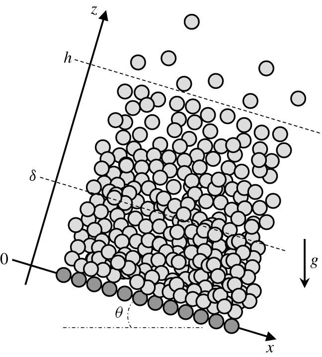
We consider an inclined flow of identical spheres of mass density  $\unicode[STIX]{x1D70C}_{p}$ and diameter
 $d$ in the presence of gravity over a rigid, bumpy base between two vertical, flat, frictional sidewalls, separated by a distance
 $W$. We take
 $x$ and
 $z$ to be the directions parallel and perpendicular to the base, in the plane parallel to the sidewalls, with the
 $x$-axis inclined of an angle
 $\unicode[STIX]{x1D703}$ with respect to the horizontal. The gravitational acceleration is
 $g$. We specify the mass of particles per unit basal area, i.e. the mass hold-up,
 ${\mathcal{M}}$, assume that the flow is fully developed and steady and perform averaging along the spanwise direction. This permits us to treat the flow as varying only in the
 $z$-direction. The only non-zero component of the spanwise-averaged particle velocity is the
 $x$-component,
 $u$. The rigid base is taken sufficiently bumpy to enforce a no-slip boundary condition for the velocity there. We take
 ${\mathcal{M}}$ large enough to permit the presence of a region of creep, which we call erodible bed, extending for a distance
 $\unicode[STIX]{x1D6FF}$ from the base.
Berzi et al. (Reference Berzi, Jenkins and Richard2019) have recently shown that, in the erodible bed, the volume fraction exceeds the critical, that is,  $\unicode[STIX]{x1D708}>\unicode[STIX]{x1D708}_{c}$; so that spheres are in ephemeral contact or experience repeating collisions along the axis of greatest compression of the flow. Above the bed and up to
 $z=h$, the solid volume fraction is less than
 $\unicode[STIX]{x1D708}_{c}$, so that the mean inter-particle distance is larger than zero; grains interact through collisions, and experience free flight in between consecutive encounters. This is the collisional flow region. For
 $z>h$, particles follow ballistic trajectories and rarely interact with other particles (Haff Reference Haff1983; Richard et al. Reference Richard, Valance, Métayer, Sanchez, Crassous, Louge and Delannay2008). In this dilute, ballistic layer, the constitutive relations of kinetic theory do not apply, because it is not possible to disregard the influence of gravity between collisions. As in Pasini & Jenkins (Reference Pasini and Jenkins2005), we identify
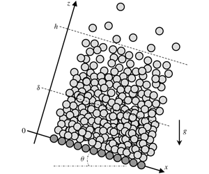
 $h$ as the distance from the base at which the length of the average ballistic trajectory equals the mean free path of kinetic theory. The flow configuration is depicted in figure 1. In the following, we make all quantities dimensionless using the particle mass density and diameter, and the gravitational acceleration; for simplicity, we do not change the notation.
Flow configuration.

2.1 Collisional flow region
For  $\unicode[STIX]{x1D6FF}<z\leqslant h$,
 $\unicode[STIX]{x1D708}<\unicode[STIX]{x1D708}_{c}$, and, because the mean inter-particle distance is greater than zero, stresses originate only from momentum exchange in collisions. Given that the particles are soft, the contact duration is not zero, so that kinetic theory for rigid particles over-estimate the actual collision frequency. Consequently, we employ the constitutive relations for the pressure
 $p$ and the shear stress
 $s$ in case of rigid particles (Garzó & Dufty Reference Garzó and Dufty1999; Vescovi et al. Reference Vescovi, Berzi, Richard and Brodu2014) but multiply them by a correction factor equal to the ratio of the time of free flight and the sum of time of free flight and contact duration (Berzi & Jenkins Reference Berzi and Jenkins2015):
 $$\begin{eqnarray}p=f_{1}T\left(1+\frac{12}{5}G\frac{T^{1/2}}{k_{n}^{1/2}}\right)^{-1}\end{eqnarray}$$
and
 $$\begin{eqnarray}s=f_{2}T^{1/2}\left(1+\frac{12}{5}G\frac{T^{1/2}}{k_{n}^{1/2}}\right)^{-1}u^{\prime }.\end{eqnarray}$$
Here and in what follows, a prime indicates derivative with respect to  $z$. The coefficients
 $f_{1}$ and
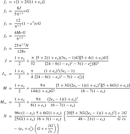
 $f_{2}$ are given in table 1, where
 $G=\unicode[STIX]{x1D708}\unicode[STIX]{x1D712}_{0}$. The term between parentheses in (2.1) and (2.2) is the correction due to the non-zero contact duration; it is valid when the contact force can be modelled as a linear spring–dashpot system, in which
 $k_{n}$ is the dimensionless spring stiffness in the normal direction.
List of auxiliary coefficients in the constitutive relations of EKT.

For the radial distribution function at contact  $\unicode[STIX]{x1D712}_{0}$, it is common to employ that of Carnahan & Starling (Reference Carnahan and Starling1969) for
 $\unicode[STIX]{x1D708}<0.49$, the freezing volume fraction,
 $$\begin{eqnarray}\unicode[STIX]{x1D712}_{0}=\frac{2-\unicode[STIX]{x1D708}}{2(1-\unicode[STIX]{x1D708})^{3}},\end{eqnarray}$$
and that of Torquato (Reference Torquato1995) for  $0.49\leqslant \unicode[STIX]{x1D708}<\unicode[STIX]{x1D708}_{c}$,
 $$\begin{eqnarray}\unicode[STIX]{x1D712}_{0}=\frac{2-0.49}{2(1-0.49)^{3}}\frac{\unicode[STIX]{x1D708}_{c}-0.49}{\unicode[STIX]{x1D708}_{c}-\unicode[STIX]{x1D708}}.\end{eqnarray}$$
Here, for computational convenience, we employ the expression suggested by Vescovi et al. (Reference Vescovi, Berzi, Richard and Brodu2014), that is, equation (2.3) for  $\unicode[STIX]{x1D708}<0.4$, and
 $$\begin{eqnarray}\unicode[STIX]{x1D712}_{0}=\left[1-\left(\frac{\unicode[STIX]{x1D708}-0.4}{\unicode[STIX]{x1D708}_{c}-0.4}\right)^{2}\right]\frac{2-\unicode[STIX]{x1D708}}{2(1-\unicode[STIX]{x1D708})^{3}}+\left(\frac{\unicode[STIX]{x1D708}-0.4}{\unicode[STIX]{x1D708}_{c}-0.4}\right)^{2}\frac{2}{\unicode[STIX]{x1D708}_{c}-\unicode[STIX]{x1D708}}\end{eqnarray}$$
for  $0.4\leqslant \unicode[STIX]{x1D708}<\unicode[STIX]{x1D708}_{c}$. The form (2.5) has the advantage of being continuously differentiable, unlike that of (2.4). This facilitates convergence in the search for numerical solutions.
As  $\unicode[STIX]{x1D708}$ approaches
 $\unicode[STIX]{x1D708}_{c}$,
 $\unicode[STIX]{x1D712}_{0}$ and, consequently,
 $G$ tend to infinity. In that limit, the coefficients
 $f_{1}$ and
 $f_{2}$ are proportional to
 $G$ and also tend to infinity. In the case of rigid particles, the scaled stresses
 $p/T$ and
 $s/(T^{1/2}u^{\prime })$ are singular at
 $\unicode[STIX]{x1D708}=\unicode[STIX]{x1D708}_{c}$, and a random, collisional assembly of rigid particles at volume fractions larger than the critical cannot exist. If the particle stiffness is finite, however, the collision frequency is proportional to the inverse of the contact duration at the critical volume fraction (Berzi & Jenkins Reference Berzi and Jenkins2015) and the scaled stresses remain finite at
 $\unicode[STIX]{x1D708}=\unicode[STIX]{x1D708}_{c}$.
The balance of fluctuation energy governs the distribution of granular temperature. In it, at steady conditions, the fluctuation energy produced through the work of the shear stress is either dissipated in collisions or diffused via velocity fluctuations. The latter term can be expressed as the divergence of the flux of fluctuation energy. Consequently, constitutive relations for the rate of collisional dissipation,  $\unicode[STIX]{x1D6E4}$, and the
 $z$-component of the flux of fluctuation energy,
 $Q$, must be provided. By modifying the expressions valid for rigid particles (Garzó & Dufty Reference Garzó and Dufty1999; Vescovi et al. Reference Vescovi, Berzi, Richard and Brodu2014) with the correction due to the finite duration of contacts (Berzi & Jenkins Reference Berzi and Jenkins2015), we obtain
 $$\begin{eqnarray}\unicode[STIX]{x1D6E4}=\frac{f_{3}}{L}T^{3/2}\left(1+\frac{12}{5}G\frac{T^{1/2}}{k_{n}^{1/2}}\right)^{-1}\end{eqnarray}$$
and
 $$\begin{eqnarray}Q=-f_{4}T^{1/2}\left(1+\frac{12}{5}G\frac{T^{1/2}}{k_{n}^{1/2}}\right)^{-1}T^{\prime }-f_{5}T^{3/2}\left(1+\frac{12}{5}G\frac{T^{1/2}}{k_{n}^{1/2}}\right)^{-1}\unicode[STIX]{x1D708}^{\prime },\end{eqnarray}$$
respectively, where  $f_{3}$,
 $f_{4}$ and
 $f_{5}$ are given in table 1.
The quantity  $\unicode[STIX]{x1D716}$ in the coefficient
 $f_{3}$ of the collisional dissipation rate (table 1) is an effective coefficient of restitution that accounts for frictional dissipation. Given the values of
 $e_{n}$,
 $e_{t}$ and
 $\unicode[STIX]{x1D707}$,
 $\unicode[STIX]{x1D716}$ can be calculated using the numerical procedure explained in the Appendix of Larcher & Jenkins (Reference Larcher and Jenkins2013).
In (2.6),  $L$ is the correlation length, which decreases the rate of collisional dissipation due to correlated motion of particles that occurs at solid volume fractions exceeding that of freezing (Jenkins Reference Jenkins2007; Mitarai & Nakanishi Reference Mitarai and Nakanishi2007; Kumaran Reference Kumaran2009). When the assumption of molecular chaos is valid,
 $L$ is equal to one diameter. Jenkins (Reference Jenkins2007), based on heuristic arguments, suggested using
 $$\begin{eqnarray}L=\max \left(1,f_{0}\frac{|u^{\prime }|}{T^{1/2}}\right),\end{eqnarray}$$
where  $f_{0}$ is a function of solid volume fraction and, through
 $\unicode[STIX]{x1D716}$, the coefficients of normal and tangential restitution and surface friction (Berzi Reference Berzi2014; Berzi & Vescovi Reference Berzi and Vescovi2015)
 $$\begin{eqnarray}f_{0}=\left[\frac{2J}{15(1-\unicode[STIX]{x1D716}^{2})}\right]^{1/2}\left[1+\frac{26(1-\unicode[STIX]{x1D716})}{15}\frac{\unicode[STIX]{x1D708}-0.49}{0.64-\unicode[STIX]{x1D708}}\right]^{3/2}.\end{eqnarray}$$
2.2 Erodible bed
At volume fractions larger than the critical, there is always some contact between spheres. This provides rate-independent components of the stresses that are associated with force transmission through a contact network. However, collisions do persist and are responsible for the rate-dependent components of the stresses.
We have recently shown (Berzi et al. Reference Berzi, Jenkins and Richard2019) that granular, erodible beds bounded by collisional flows are fragile, in the sense that, there, the average number of contacts per particle is less than the critical value required for mechanical stability (Silbert Reference Silbert2010; Sun & Sundaresan Reference Sun and Sundaresan2011). As a consequence, the bulk stiffness of erodible beds (Berzi et al. Reference Berzi, Jenkins and Richard2019) is three orders of magnitude less than that measured in homogeneous shearing flows at the same volume fraction (Chialvo et al. Reference Chialvo, Sun and Sundaresan2012; Berzi & Jenkins Reference Berzi and Jenkins2015).
As in the case of homogeneous shearing for  $\unicode[STIX]{x1D708}$ larger than
 $\unicode[STIX]{x1D708}_{c}$ (Berzi & Jenkins Reference Berzi and Jenkins2015), we take the pressure and the shear stress in the bed equal to
 $$\begin{eqnarray}p={\textstyle \frac{5}{6}}(1+e_{n})\unicode[STIX]{x1D708}k_{n}^{1/2}T^{1/2}+0.0006(\unicode[STIX]{x1D708}-\unicode[STIX]{x1D708}_{c})k_{n}\end{eqnarray}$$
and
 $$\begin{eqnarray}\frac{s}{p}=\frac{4J_{\infty }}{5\unicode[STIX]{x03C0}^{1/2}(1+e_{n})}\frac{u^{\prime }}{T^{1/2}},\end{eqnarray}$$
where  $J_{\infty }$ is given in table 1. In (2.10), the first term on the right-hand side is the rate-dependent component, in which the strength of collisions is influenced by the elasticity of the contacts; the second term is the rate-independent component. In the latter, the coefficient of proportionality with the normal spring stiffness is three orders of magnitude less than the value 0.6 appropriate for homogeneous shearing, in accord with the observations of Berzi et al. (Reference Berzi, Jenkins and Richard2019) on the fragility of the force chains in erodible beds.
Given that collisions do persist in the erodible bed, we adopt the constitutive relations for the collisional dissipation rate and the fluctuation energy flux suggested by Berzi & Jenkins (Reference Berzi and Jenkins2015) for dense, shearing flows of soft particles above the critical volume fraction
 $$\begin{eqnarray}\unicode[STIX]{x1D6E4}=\frac{5(1-\unicode[STIX]{x1D716}^{2})\unicode[STIX]{x1D708}}{\unicode[STIX]{x03C0}^{1/2}L_{c}}k_{n}^{1/2}T\end{eqnarray}$$
and
 $$\begin{eqnarray}Q=-\frac{5M_{\infty }\unicode[STIX]{x1D708}}{3\unicode[STIX]{x03C0}^{1/2}}k_{n}^{1/2}T^{\prime },\end{eqnarray}$$
where  $M_{\infty }$ is given in table 1. In writing (2.13), we have ignored the dependence of the energy flux on
 $\unicode[STIX]{x1D708}^{\prime }$ while retaining the dependence on
 $T^{\prime }$. We have determined that its inclusion, apart from complicating the mathematics, has no effect on the predictions of the theory reported in the next sections. In (2.13),
 $L_{c}$ is the correlation length when
 $\unicode[STIX]{x1D708}$ exceeds
 $\unicode[STIX]{x1D708}_{c}$. Berzi & Jenkins (Reference Berzi and Jenkins2015) showed that
 $$\begin{eqnarray}L_{c}=1+\frac{26(1-\unicode[STIX]{x1D716})}{15}\frac{\unicode[STIX]{x1D708}_{c}-0.49}{0.64-\unicode[STIX]{x1D708}_{c}};\end{eqnarray}$$
that is, a constant, which contributes to the reproduction of the results in steady, homogeneous shearing flows, also recently confirmed by direct measurements in numerical simulations (Oyama, Mizuno & Saitoh Reference Oyama, Mizuno and Saitoh2019).
3 Boundary-value problem
In order to obtain profiles of solid volume fraction, granular temperature,  $x$-velocity and stresses and to quantitatively compare predictions of EKT with DEM simulations of steady, confined, incline flows over erodible beds, we have to employ balances of momentum and fluctuation energy. These, together with the constitutive relations introduced in the previous section, permit the formulation of a set of differential equations whose solution requires boundary conditions. In doing this, we distinguish between the collisional flow, where the pressure is larger than in the ballistic layer above it and the solid volume fraction is less than the critical, and the erodible bed, where the solid volume fraction exceeds
 $\unicode[STIX]{x1D708}_{c}$.
3.1 Collisional flow region
In the collisional flow region, the spanwise-averaged momentum balances along the  $z$ and
 $x$-directions for steady and fully developed inclined flows in the presence of sidewalls are (Jenkins & Berzi Reference Jenkins and Berzi2010; Gollin et al. Reference Gollin, Berzi and Bowman2017)
 $$\begin{eqnarray}p^{\prime }=-\unicode[STIX]{x1D708}\cos \unicode[STIX]{x1D703}\end{eqnarray}$$
and
 $$\begin{eqnarray}s^{\prime }=-\unicode[STIX]{x1D708}\sin \unicode[STIX]{x1D703}+2\frac{\unicode[STIX]{x1D707}_{w}}{W}p,\end{eqnarray}$$
respectively, where  $\unicode[STIX]{x1D707}_{w}$ is an effective wall friction coefficient, which accounts for the average force exerted by the sidewalls on the flow (Taberlet et al. Reference Taberlet, Richard, Valance, Losert, Pasini, Jenkins and Delannay2003). We take
 $\unicode[STIX]{x1D707}_{w}=\unicode[STIX]{x1D707}[1-\exp (-0.14u/T^{1/2})]$. The reasoning for this is provided in appendix A. Equations (3.1) and (3.2) assume that the normal stresses are isotropic and equal to the pressure. Departures from this assumption are discussed in appendix B.
In steady, inhomogeneous flows, the balance of the fluctuation kinetic energy is
 $$\begin{eqnarray}su^{\prime }=Q^{\prime }+\unicode[STIX]{x1D6E4},\end{eqnarray}$$
where the term on the left-hand side represents the energy produced through the work of the shear stress, while  $Q^{\prime }$ is the energy diffusion due the velocity fluctuations of the particles. We ignore the possible flux of energy to or from the walls due to the possible imbalance between the working of the wall shear stress through the span-averaged flow velocity and the rate of dissipation of energy in wall collisions (Jenkins Reference Jenkins1992). We have checked that its inclusion has negligible effects on the results.
For inhomogeneous flows in which the volume fraction is greater than 0.49, the balance of energy corresponds to the non-local, linear equation introduced for the fluidity by Kamrin and coworkers (Kamrin & Koval Reference Kamrin and Koval2012; Kamrin & Henann Reference Kamrin and Henann2015; Zhang & Kamrin Reference Zhang and Kamrin2017). In such flows, the energy balance can be written as a linear equation for  $T^{1/2}$, similar to that at lesser densities (e.g. Jenkins Reference Jenkins1994), and Zhang & Kamrin (Reference Zhang and Kamrin2017) have recently shown that this measure of the strength of the velocity fluctuations and the fluidity are equivalent.
In (3.1), (3.2) and (3.3), we use the constitutive relations of EKT for random aggregates of soft particles, i.e. (2.1), (2.2), (2.6) and (2.7). This permits us to use a value of the solid volume fraction arbitrarily close to  $\unicode[STIX]{x1D708}_{c}$ as a boundary condition at the interface with the erodible bed.
We differentiate (2.1) with respect to  $z$ and use it in (3.1) and (2.7) to obtain the differential equation governing the distribution of the solid volume fraction in the collisional flow
 $$\begin{eqnarray}\unicode[STIX]{x1D708}^{\prime }=\left[\frac{\unicode[STIX]{x2202}p}{\unicode[STIX]{x2202}T}\left(1+\frac{12}{5}G\frac{w}{k_{n}^{1/2}}\right)Q-f_{4}w\unicode[STIX]{x1D708}\cos \unicode[STIX]{x1D703}\right]\left(\frac{\unicode[STIX]{x2202}p}{\unicode[STIX]{x2202}\unicode[STIX]{x1D708}}f_{4}w-\frac{\unicode[STIX]{x2202}p}{\unicode[STIX]{x2202}T}\,f_{5}w^{3}\right)^{-1},\end{eqnarray}$$
where  $w=T^{1/2}$,
 $$\begin{eqnarray}\frac{\unicode[STIX]{x2202}p}{\unicode[STIX]{x2202}T}=f_{1}\left(1+\frac{12}{5}G\frac{w}{k_{n}^{1/2}}\right)^{-1}-\frac{1}{2}f_{1}\frac{12}{5}G\frac{w}{k_{n}^{1/2}}\left(1+\frac{12}{5}G\frac{w}{k_{n}^{1/2}}\right)^{-2}\end{eqnarray}$$
and
 $$\begin{eqnarray}\frac{\unicode[STIX]{x2202}p}{\unicode[STIX]{x2202}\unicode[STIX]{x1D708}}=\frac{\unicode[STIX]{x2202}f_{1}}{\unicode[STIX]{x2202}\unicode[STIX]{x1D708}}w^{2}\left(1+\frac{12}{5}G\frac{w}{k_{n}^{1/2}}\right)^{-1}-f_{1}w^{2}\frac{12}{5}\frac{\unicode[STIX]{x2202}G}{\unicode[STIX]{x2202}\unicode[STIX]{x1D708}}\frac{w}{k_{n}^{1/2}}\left(1+\frac{12}{5}G\frac{w}{k_{n}^{1/2}}\right)^{-2}.\end{eqnarray}$$
The differential equation that governs the distribution of the shear stress (3.2) becomes, with (2.1) and the expression for  $\unicode[STIX]{x1D707}_{w}$,
 $$\begin{eqnarray}s^{\prime }=-\unicode[STIX]{x1D708}\sin \unicode[STIX]{x1D703}+2\frac{\unicode[STIX]{x1D707}}{W}\left[1-\exp \left(-0.14\frac{u}{w}\right)\right]f_{1}w^{2}\left(1+\frac{12}{5}G\frac{w}{k_{n}^{1/2}}\right)^{-1}.\end{eqnarray}$$
Equation (2.2) gives
 $$\begin{eqnarray}u^{\prime }=\frac{1}{f_{2}}\frac{s}{w}\left(1+\frac{12}{5}G\frac{w}{k_{n}^{1/2}}\right).\end{eqnarray}$$
The differential equation for the  $z$-component of the energy flux (3.3) becomes, with (2.6) and (3.8),
 $$\begin{eqnarray}Q^{\prime }=\frac{1}{f_{2}}\frac{s^{2}}{w}\left(1+\frac{12}{5}G\frac{w}{k_{n}^{1/2}}\right)-\frac{f_{3}}{L}w^{3}\left(1+\frac{12}{5}G\frac{w}{k_{n}^{1/2}}\right)^{-1},\end{eqnarray}$$
where  $L$ is given in (2.8). The governing equation for the distribution of the square root of the granular temperature is given by (2.7) and (3.4):
 $$\begin{eqnarray}\displaystyle w^{\prime } & = & \displaystyle -\frac{Q}{2f_{4}w^{2}}\left(1+\frac{12}{5}G\frac{w}{k_{n}^{1/2}}\right)\nonumber\\ \displaystyle & & \displaystyle -\,\frac{f_{5}}{2f_{4}}w\left[\frac{\unicode[STIX]{x2202}p}{\unicode[STIX]{x2202}T}\left(1+\frac{12}{5}G\frac{w}{k_{n}^{1/2}}\right)Q-f_{4}w\unicode[STIX]{x1D708}\cos \unicode[STIX]{x1D703}\right]\left(\frac{\unicode[STIX]{x2202}p}{\unicode[STIX]{x2202}\unicode[STIX]{x1D708}}f_{4}w-\frac{\unicode[STIX]{x2202}p}{\unicode[STIX]{x2202}T}f_{5}w^{3}\right)^{-1}\!.\qquad\end{eqnarray}$$
Finally, as in Jenkins & Berzi (Reference Jenkins and Berzi2010) and Gollin et al. (Reference Gollin, Berzi and Bowman2017), we define the partial mass hold-up,  $m=\int _{0}^{z}\unicode[STIX]{x1D708}\,\text{d}z$. The differential equation for the partial mass hold-up is, then,
 $$\begin{eqnarray}m^{\prime }=\unicode[STIX]{x1D708}.\end{eqnarray}$$
We require boundary conditions at the top and bottom of the collisional flow. As already mentioned, Pasini & Jenkins (Reference Pasini and Jenkins2005) identified the interface with the ballistic layer, that is  $z=h$, as the position at which twice the height of a ballistic trajectory,
 $3T$, is equal to the mean free path of kinetic theory,
 $\sqrt{2}/(12\unicode[STIX]{x1D708})$ (Chapman et al. Reference Chapman, Cowling and Burnett1990). With this and (2.1),
 $$\begin{eqnarray}p_{h}=0.039,\end{eqnarray}$$
where, here and in what follows, the subscript indicates the location at which that quantity is evaluated. At  $z=h$, the shear stress and the energy flux have been derived by Jenkins & Hanes (Reference Jenkins and Hanes1993) as
 $$\begin{eqnarray}s_{h}=p_{h}\tan \unicode[STIX]{x1D703}\end{eqnarray}$$
and
 $$\begin{eqnarray}Q_{h}=-p_{h}w_{h}\tan ^{2}\unicode[STIX]{x1D703},\end{eqnarray}$$
respectively. Finally, we neglect the contribution of the ballistic layer to the mass hold-up and take
 $$\begin{eqnarray}m_{h}={\mathcal{M}}.\end{eqnarray}$$
At the interface with the erodible bed,  $z=\unicode[STIX]{x1D6FF}$, as mentioned, we take
 $\unicode[STIX]{x1D708}_{\unicode[STIX]{x1D6FF}}$ arbitrarily close to
 $\unicode[STIX]{x1D708}_{c}$.
3.2 Erodible bed
In the bed, where  $\unicode[STIX]{x1D708}$ exceeds
 $\unicode[STIX]{x1D708}_{c}$, we use the constitutive relations (2.11) through (2.14). This implies that velocity fluctuations are also crucial in the erodible bed, where we assume that ‘the fluctuating energy supplied at the interface’ with the flow region is ‘conducted away from this surface, dissipated in collisions and eventually disappears’ (Jenkins & Askari Reference Jenkins and Askari1991). That is, because the shear rate is negligible in the bed, we ignore the production of fluctuation energy associated with it, and assume that the diffusion of fluctuation energy equals its dissipation
 $$\begin{eqnarray}-Q^{\prime }=\unicode[STIX]{x1D6E4}.\end{eqnarray}$$
The momentum balances (3.1) and (3.2) continue to apply in the bed, with the effective wall friction coefficient depending on the ratio  $u/T^{1/2}$ as in the collisional flow. We differentiate (2.10) with respect to
 $z$ and use it in (3.1) and (2.13) to obtain the differential equation governing the distribution of the solid volume fraction in the bed:
 $$\begin{eqnarray}\unicode[STIX]{x1D708}^{\prime }=\left[\frac{\unicode[STIX]{x03C0}^{1/2}(1+e_{n})Q}{4M_{\infty }w}-\unicode[STIX]{x1D708}\cos \unicode[STIX]{x1D703}\right]\left[\frac{5}{6}(1+e_{n})k_{n}^{1/2}w+0.0006k_{n}\right]^{-1}.\end{eqnarray}$$
We obtain the differential equation governing the distribution of the shear stress in the bed from (3.2), with (2.10) and the expression for  $\unicode[STIX]{x1D708}_{w}$:
 $$\begin{eqnarray}s^{\prime }=-\unicode[STIX]{x1D708}\sin \unicode[STIX]{x1D703}+2\frac{\unicode[STIX]{x1D707}}{W}\left[1-\exp \left(-0.14\frac{u}{w}\right)\right]\left[\frac{5}{6}(1+e_{n})\unicode[STIX]{x1D708}k_{n}^{1/2}w+0.0006(\unicode[STIX]{x1D708}-\unicode[STIX]{x1D708}_{c})k_{n}\right].\end{eqnarray}$$
We obtain the shear rate in the bed from (2.11) and (2.10):
 $$\begin{eqnarray}u^{\prime }=\frac{5\unicode[STIX]{x03C0}^{1/2}(1+e_{n})}{4J_{\infty }}sw\left[\frac{5}{6}(1+e_{n})\unicode[STIX]{x1D708}k_{n}^{1/2}w+0.0006(\unicode[STIX]{x1D708}-\unicode[STIX]{x1D708}_{c})k_{n}\right]^{-1}.\end{eqnarray}$$
The distribution of the  $z$-component of the energy flux in the bed is governed by (3.16) with (2.12),
 $$\begin{eqnarray}Q^{\prime }=-\frac{5(1-\unicode[STIX]{x1D716}^{2})\unicode[STIX]{x1D708}}{\unicode[STIX]{x03C0}^{1/2}L_{c}}k_{n}^{1/2}w^{2},\end{eqnarray}$$
with  $L_{c}$ given in (2.14). The differential equation for the square root of the granular temperature in the bed is, from (2.13),
 $$\begin{eqnarray}w^{\prime }=-\frac{3\unicode[STIX]{x03C0}^{1/2}Q}{10\unicode[STIX]{x1D708}M_{\infty }k_{n}^{1/2}w}.\end{eqnarray}$$
Finally, the differential equation governing the distribution of the partial mass hold-up in the erodible bed is
 $$\begin{eqnarray}m^{\prime }=\unicode[STIX]{x1D708}\end{eqnarray}$$
as in the collisional flow.
The bottom of the bed, at  $z=0$, is in contact with a rough, rigid base. There, we assume the no-slip boundary condition
 $$\begin{eqnarray}u_{0}=0;\end{eqnarray}$$
that there is no energy flux injected into or taken from the particles in the bed
 $$\begin{eqnarray}Q_{0}=0;\end{eqnarray}$$
and that
 $$\begin{eqnarray}m_{0}=0.\end{eqnarray}$$
Equations (3.4), (3.7) through (3.11), and (3.17) through (3.22) are a system of 12 differential equations in the 6 variables  $\unicode[STIX]{x1D708}$,
 $s$,
 $u$,
 $Q$,
 $w$ and
 $m$ evaluated in the collisional flow and in the bed (12 unknowns). We solve this system using the Matlab ‘bvp4c’ two-point boundary-value problem solver with the boundary conditions (3.12) through (3.15), (3.23) through (3.25),
 $\unicode[STIX]{x1D708}_{\unicode[STIX]{x1D6FF}}\approx \unicode[STIX]{x1D708}_{c}$ and assuming continuity in all six variables at the interface between the collisional flow and the bed (14 boundary conditions). The two additional boundary conditions allow the values of the thicknesses of the collisional flow,
 $h-\unicode[STIX]{x1D6FF}$, and of the bed itself,
 $\unicode[STIX]{x1D6FF}$, to be determined as part of the solution.
Given that the differential equations are highly nonlinear, the convergence of the iteration process towards the numerical solution of the system is somewhat delicate; the initial guess for the distribution of the unknowns must be sufficiently close to the eventual solution. The Matlab code employed for the solution of the differential equations and values of the variables that can be used as initial guess are available at http://intranet.dica.polimi.it/people/berzi-diego/.
4 Comparisons with discrete numerical simulations
We now compare the distributions of various quantities along the  $z$-direction obtained from the solution to the two-point boundary value problem with those measured in DEM simulations of inclined flows of inelastic, frictional spheres between frictional sidewalls (author’s unpublished observations). The discrete-element method is based on the soft-sphere approach. The basic principle of DEM simulations is to treat the particles as spheres (the size of the particles is mildly poly-dispersed, ±20 %, to avoid crystallization) submitted to gravity and contact forces with both other particles and boundaries. These contact forces are described by the well-known linear spring–dashpot force model in both normal (spring stiffness
 $k_{n}$, damping
 $\unicode[STIX]{x1D6FE}_{n}$) and tangential directions (spring stiffness
 $k_{t}$, damping
 $\unicode[STIX]{x1D6FE}_{t}$). In the tangential direction, the spring elongation is truncated to satisfy Coulomb’s law. The following values of the dimensionless parameters are used:
 $k_{n}=2.94\times 10^{6}$,
 $k_{t}=2k_{n}/7$,
 $\unicode[STIX]{x1D6FE}_{t}=0$ and coefficient of sliding friction
 $\unicode[STIX]{x1D707}=0.5$. The value of
 $\unicode[STIX]{x1D6FE}_{n}$ is adjusted to obtain the desired value of the normal restitution coefficient,
 $e_{n}=0.88$, while the tangential coefficient of restitution is
 $e_{t}=1$. The dimensionless stiffness, in units of
 $\unicode[STIX]{x1D70C}_{p}gd^{2}$, employed in the DEM simulations is approximately three orders of magnitude less that the dimensionless stiffness of 1 mm glass spheres, with a Young’s modulus of the order of 70 GPa.
The simulation chute is a rectangular cuboid which can be inclined relatively to the horizontal by the angle  $\unicode[STIX]{x1D703}$. Its size in the
 $x$-direction is equal to 25.3, with periodic boundary conditions employed along this direction. Along the
 $z$-direction (i.e. normal to the free surface of the flow), the size of the cell is considered as infinite. Frictional sidewalls are located at positions
 $y=-W/2$ and
 $y=W/2$. They are treated as sphere of infinite radius and mass. Initially, the angle of inclination is set to a large value,
 $\unicode[STIX]{x1D703}\approx 70^{\circ }$, and grains are poured in the system from an ordered, slightly dilute, hexagonal compact packing.
Each component of the dimensionless grains’ velocity is initially randomly and uniformly assigned between  $-1$ and
 $+1$. The angle was then decreased instantaneously to the desired value and the system slowly relaxes to a steady and fully developed state that has no sign of the initial ordered structure. Note that this protocol leads to relatively loose erodible beds and other protocols (e.g. by initially building a dense static packing and triggering the flow by suddenly increase the inclination angle) lead to much denser erodible bases and, thus, likely different results.
For solving the differential problem outlined in the previous section, we employ the same set of microscopic parameters of the DEM simulations. That is,  $e_{n}=0.88$,
 $e_{t}=1$,
 $\unicode[STIX]{x1D707}=0.5$ and
 $k_{n}=2.94\times 10^{6}$. Then, the effective coefficient of normal restitution
 $\unicode[STIX]{x1D716}=0.645$ (Larcher & Jenkins Reference Larcher and Jenkins2013), while
 $\unicode[STIX]{x1D708}_{c}=0.587$ (Chialvo et al. Reference Chialvo, Sun and Sundaresan2012).
The mass hold-up  ${\mathcal{M}}$, the angle of inclination,
 $\unicode[STIX]{x1D703}$, and the channel width,
 $W$, are imposed in the simulations. Here, we limit the comparisons with the simulations to
 $W=20$ and 30. In separate unpublished observations by P.R., due to the presence of the sidewalls, flows in channels of width
 $W=5$ and 10 are strongly layered in the spanwise direction. As already mentioned, all measurements in the simulations are averaged along the spanwise direction. We exclude from the analysis measurements in the region adjacent to the rigid bottom, where the solid volume fraction decreases as the base is approached. The thickness of this region is about five diameters and, within it, the base influences the coarse graining. We also exclude measurements in the ballistic layer at the top, where
 $p<0.039$ (Pasini & Jenkins Reference Pasini and Jenkins2005).
In the following, we report comparisons for three combinations of the control parameters:  ${\mathcal{M}}=25$,
 $\unicode[STIX]{x1D703}=30^{\circ }$ and
 $W=30$;
 ${\mathcal{M}}=25$,
 $\unicode[STIX]{x1D703}=25^{\circ }$ and
 $W=30$; and
 ${\mathcal{M}}=37$,
 $\unicode[STIX]{x1D703}=35^{\circ }$ and
 $W=20$. Similar agreement, not shown here for brevity, is obtained for all the DEM simulations performed with
 $W=20$ and 30 diameters (author’s unpublished observations).
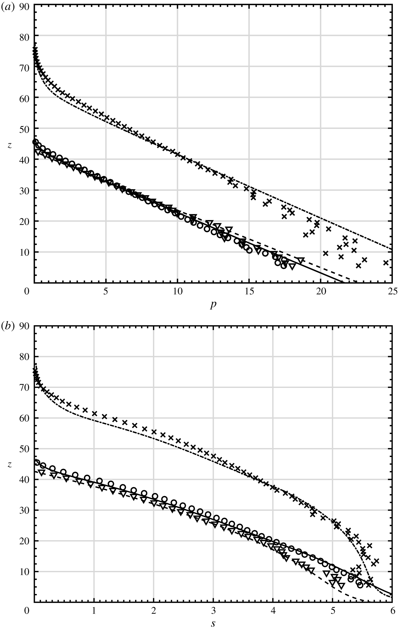
Measured (symbols) and predicted (lines) profiles of (a) pressure and (b) shear stress for:  ${\mathcal{M}}=25$,
 $\unicode[STIX]{x1D703}=30^{\circ }$ and
 $W=30$ (circles and solid line);
 ${\mathcal{M}}=25$,
 $\unicode[STIX]{x1D703}=25^{\circ }$ and
 $W=30$ (triangles and dashed line);
 ${\mathcal{M}}=37$,
 $\unicode[STIX]{x1D703}=35^{\circ }$ and
 $W=20$ (crosses and dot-dashed line).

Figure 2(a) shows that the profiles of pressure are overall well predicted by EKT (the maximum deviation from the measurements is within 10 %), even near the top, where the anisotropy in the normal stresses is strong (appendix B), and in the bed, thus justifying the validity of the constitutive relation (2.10). The pressure is overpredicted near the bottom for the case  $W=20$ and
 $\unicode[STIX]{x1D703}=35^{\circ }$, although the scattering in the measurements might point to a problem with the coarse-graining procedure there. A remarkable agreement is obtained also for the distribution of the shear stress (figure 2b). The theory correctly predicts even the deviation from the linear distribution near the bottom of the erodible bed. Obviously, this is a consequence of the validity of the expression for the dependence of the effective wall friction coefficient on the ratio
 $u/T^{1/2}$, that we fit using the measurements, even in the bed. It would have been more desirable to employ, for
 $\unicode[STIX]{x1D707}_{w}$, the expression derived from the application of the momentum balance at a flat, frictional wall (Jenkins Reference Jenkins1992), with no adjustable parameter. We claim that this is not possible because we are employing a one-dimensional approximation to an inherently two-dimensional problem. The non-trivial extension of the present theory to deal with two-dimensional flows is currently work in progress.
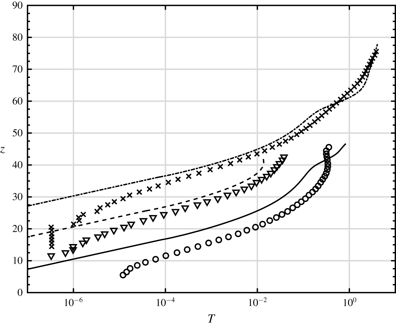
Measured (symbols) and predicted (lines) profiles of granular temperature for:  ${\mathcal{M}}=25$,
 $\unicode[STIX]{x1D703}=30^{\circ }$ and
 $W=30$ (circles and solid line);
 ${\mathcal{M}}=25$,
 $\unicode[STIX]{x1D703}=25^{\circ }$ and
 $W=30$ (triangles and dashed line);
 ${\mathcal{M}}=37$,
 $\unicode[STIX]{x1D703}=35^{\circ }$ and
 $W=20$ (crosses and dot-dashed line).

The behaviour of the granular temperature is well captured by EKT when  $W=20$ and
 $\unicode[STIX]{x1D703}=35^{\circ }$ (figure 3). For the other two cases, instead, the theory underpredicts the granular temperature. Near the top, this has probably to do with the fact that the anisotropy in the velocity fluctuations is stronger, and a linear kinetic theory that assumes nearly isotropic velocity fluctuations is not applicable. This is particularly evident for the case
 $W=30$ and
 $\unicode[STIX]{x1D703}=30^{\circ }$. We also emphasize that the boundary condition for the pressure at the top of the flow, equation (3.12), has been derived for horizontal flows in which the velocity fluctuations were taken to be isotropic. Both assumptions are violated in the present flow configurations, and this has consequences on the predictions of both the granular temperature and the solid volume fraction at the interface with the ballistic layer.
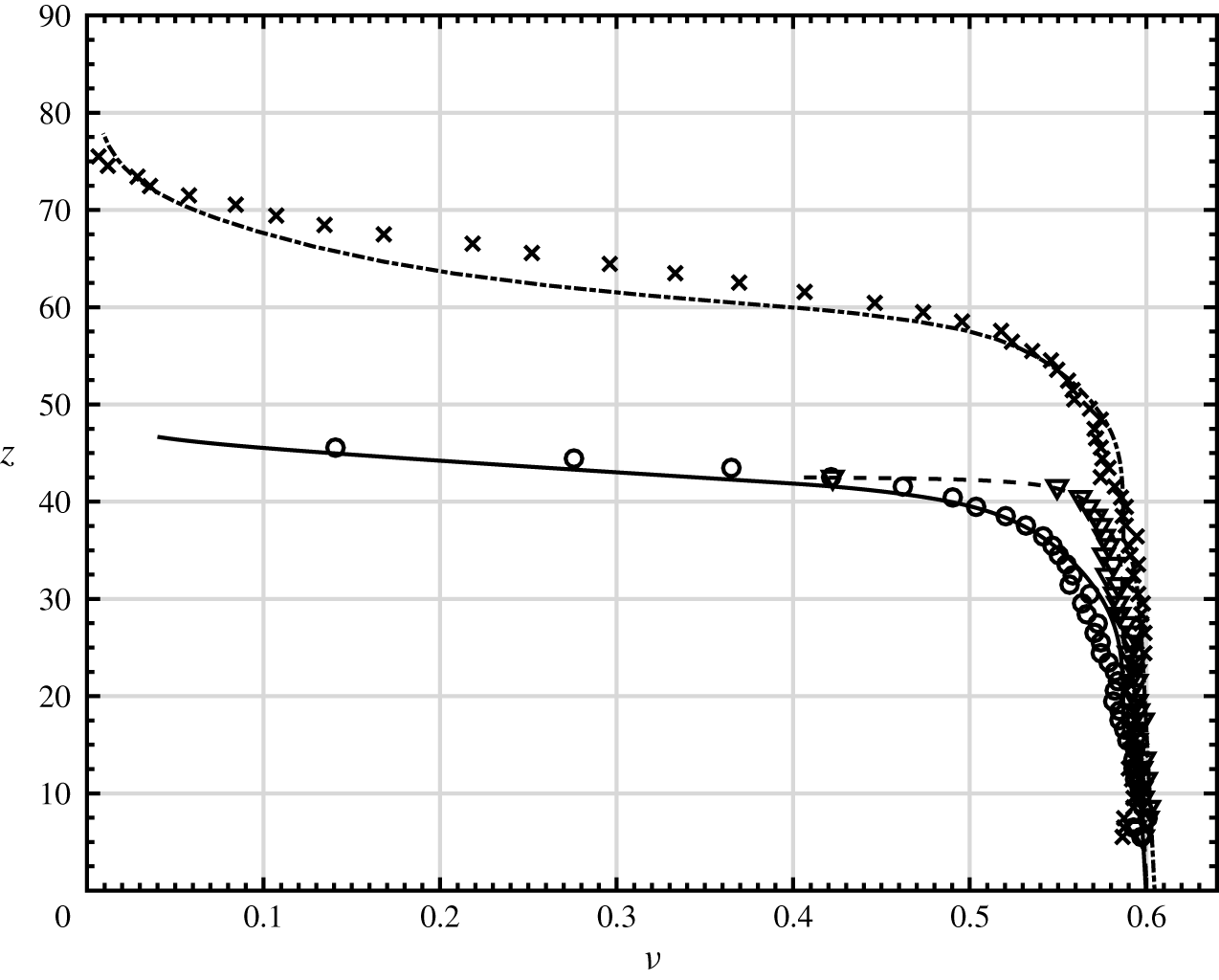
On the other hand, in the core of the flow, the solid volume fraction is slightly overpredicted (see the later figure 5). The strong dependence on  $\unicode[STIX]{x1D708}$ of the function
 $f_{1}$ in the expression for the pressure of kinetic theory, equation (2.1), implies that small deviations in the solid volume fraction result in much larger deviations in
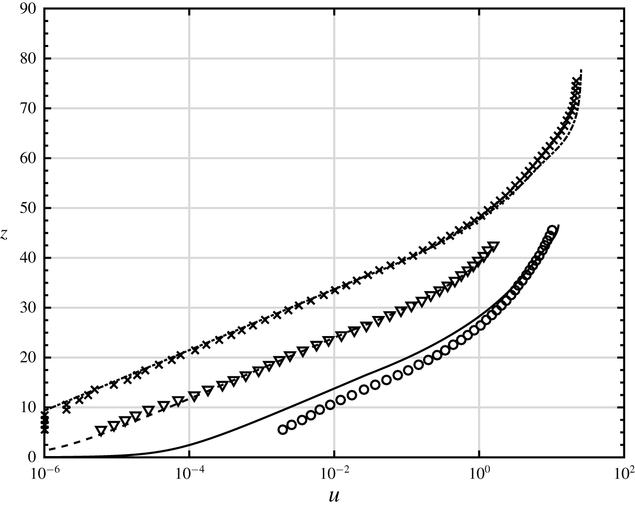
 $T$. Despite this, the exponential decay of
 $T$ inside the bed (figure 3) is notably reproduced. Near the rigid base, the measured granular temperature deviates from the exponential decay. This seems to suggest that the rigid boundary is not actually adiabatic, but acts as a source of fluctuation energy for the granular material. Capturing this behaviour, although possible by making use of different boundary conditions at the rigid base, such as those for granular flows over rigid, bumpy surfaces (Richman Reference Richman1988), would unnecessarily complicate the analysis.
Measured (symbols) and predicted (lines) profiles of  $x$-velocity for:
 ${\mathcal{M}}=25$,
 $\unicode[STIX]{x1D703}=30^{\circ }$ and
 $W=30$ (circles and solid line);
 ${\mathcal{M}}=25$,
 $\unicode[STIX]{x1D703}=25^{\circ }$ and
 $W=30$ (triangles and dashed line);
 ${\mathcal{M}}=37$,
 $\unicode[STIX]{x1D703}=35^{\circ }$ and
 $W=20$ (crosses and dot-dashed line).

The EKT can qualitatively and quantitatively reproduce the profiles of  $x$-velocity (figure 4), both in the collisional flow and in the erodible bed. The velocity is less sensitive than the granular temperature to small deviations in the solid volume fraction in the collisional flow, because its distribution is governed by the shear stress, which is well predicted, and the viscosity, which is proportional to the product of the coefficient
 $f_{2}$ of kinetic theory and the square root of the granular temperature (see (2.2)). Overestimations in
 $f_{2}$ and underestimations in
 $T$ compensate each other, so that the agreement between the theory and the measurements is remarkable. The well-known exponential decay of the velocity in the erodible bed is also notably predicted (figure 4). The fact that only non-local approaches were previously able to reproduce this feature (Kamrin & Koval Reference Kamrin and Koval2012; Zhang & Kamrin Reference Zhang and Kamrin2017), reinforces our interpretation of the non-local rheology as a special case of EKT.
Measured (symbols) and predicted (lines) profiles of solid volume fraction for:  ${\mathcal{M}}=25$,
 $\unicode[STIX]{x1D703}=30^{\circ }$ and
 $W=30$ (circles and solid line);
 ${\mathcal{M}}=25$,
 $\unicode[STIX]{x1D703}=25^{\circ }$ and
 $W=30$ (triangles and dashed line);
 ${\mathcal{M}}=37$,
 $\unicode[STIX]{x1D703}=35^{\circ }$ and
 $W=20$ (crosses and dot-dashed line).

Finally, the agreement between the predicted and measured profiles of solid volume fraction is excellent (figure 5). As anticipated, the volume fraction is slightly overpredicted in the dense region of the collisional flow, say where the volume fraction is comprised between 0.5 and  $\unicode[STIX]{x1D708}_{c}$. These small deviations, of order 1 %, are sufficient to cause the sensible deviations in the granular temperature shown in figure 3, as already pointed out. Given that the distribution (3.4) of the volume fraction depends on the fluctuation energy flux, this might suggest that the expression for the latter could be improved in future works.
5 Conclusions
We have focused on steady and fully developed, inclined, collisional shearing flows of frictional spheres confined between flat, frictional sidewalls in situations in which the number of particles in the system is sufficient to develop erodible beds. The bed is the region in which the solid volume fraction exceeds the critical value for the development of rate-independent components of the stresses. Existing results of discrete-element simulations demonstrate that the flow above the erodible bed is inherently collisional: interactions are essentially binary and stresses originate from momentum exchange in collisions. We have employed the constitutive relations of extended kinetic theory, which accounts for strong collisional inelasticity, friction, velocity correlation at volume fraction larger than the freezing point and finite duration of particle contacts, to close the balances of momentum and fluctuation energy in the collisional flow.
In the bed, rate-independent stresses proportional to the particle stiffness develop, although much weaker than the rate-independent stresses that would characterize steady and fully developed, homogeneous shearing flows at the same volume fraction. However, the numerical simulations show that velocity fluctuations do persist in the erodible bed. Assuming that the production of velocity fluctuations through the working of the shear stress is negligible in the erodible bed, taking the frequency of collisions inversely proportional to the contact duration in the expressions for the rate-dependent components of pressure and shear stress, the fluctuation energy flux and the collisional dissipation rate allowed us to obtain numerical distributions of stresses, granular temperature, velocity and volume fraction that fit well to those measured in the numerical simulations. The boundary conditions at the top of the collisional flow were already available in the literature, while we employed simple boundary conditions, no slip and zero energy flux, at the bottom of the bed. To treat the flow as unidimensional, we modelled the frictional sidewalls as additional tangential stresses. We took them as proportional to the particle pressure through a function of the local ratio between the slip velocity at the walls and the square root of granular temperature, as suggested by existing boundary conditions for the collisional flow of particles over a flat, frictional surface. In that expression there is a parameter that we fit to the measurements.
The comparisons between the numerical solution of the present model and the results of discrete numerical simulations for different values of particle mass per unit basal area, channel widths and inclinations are remarkable, given that the only parameters of the model are the coefficients of normal and tangential restitution, sliding friction, normal stiffness, and the fitting parameter in the expression for the effective wall friction coefficient. Extensions of the theory to fully two-dimensional flows should eliminate the need for the latter. The limited number of physically accessible parameters of the model and its capability of reproducing distributions of stresses, volume fractions, velocity and granular temperature, ranging from dilute to extremely dense conditions, are strong arguments in favour of EKT when dealing with granular flows. It remains to better understand the nature of the erodible bed, in particular its micro-structure, in relation to both the constitutive relations for the stresses and the balance of fluctuation energy there.
Declaration of interests
The authors report no conflict of interest.
Appendix A. Effective wall friction
In (3.2), the effective wall friction coefficient is usually taken to be constant (Taberlet et al. Reference Taberlet, Richard, Valance, Losert, Pasini, Jenkins and Delannay2003; Jop et al. Reference Jop, Forterre and Pouliquen2005; Jenkins & Berzi Reference Jenkins and Berzi2010; Gollin et al. Reference Gollin, Berzi and Bowman2017), for simplicity. If all particle–wall contacts are sliding,  $\unicode[STIX]{x1D707}_{w}$ would be equal to the actual wall–particle sliding friction coefficient, i.e. 0.5 in the DEM simulations of (author’s unpublished observations). However, it has been shown that
 $\unicode[STIX]{x1D707}_{w}$ is not constant and actually decreases towards the erodible bed (Richard et al. Reference Richard, Valance, Métayer, Sanchez, Crassous, Louge and Delannay2008), because, as the bed is approached, rolling contacts between the particles and the walls become dominant.
Boundary conditions for the flows of grains over a flat, frictional surface have been derived in the context of kinetic theory (Jenkins Reference Jenkins1992). There, the slip velocity of the point of contact between the particles and the wall scaled by the square root of the granular temperature is related to the ratio of the normal to the tangential stress at the wall, through a function of the normal and tangential coefficients of restitution and the coefficient of sliding friction. Jenkins (Reference Jenkins1992) obtained
 $$\begin{eqnarray}\unicode[STIX]{x1D707}_{w}=\min \left(\frac{\sqrt{3}}{7}\frac{1+e_{t}}{1+e_{n}}\frac{u}{T^{1/2}},\unicode[STIX]{x1D707}\right),\end{eqnarray}$$
which is a combination of two limits: no sliding (all rolling) for small  $u/T^{1/2}$ and all sliding (no rolling) for large
 $u/T^{1/2}$. To better capture the transition between those two extremes, Louge (Reference Louge1994) suggested a fit of the form
 $$\begin{eqnarray}\unicode[STIX]{x1D707}_{w}=\unicode[STIX]{x1D707}\left[1-\exp \left(-C\frac{u}{T^{1/2}}\right)\right],\end{eqnarray}$$
where  $C$ is a constant that depends on
 $e_{n}$,
 $e_{t}$ and
 $\unicode[STIX]{x1D707}$. With the restitution and friction coefficients of the DEM simulations (author’s unpublished observations), we obtain
 $C=0.46$. However, the analysis of Louge (Reference Louge1994) was limited to values of
 $\unicode[STIX]{x1D707}\leqslant 0.4$ and
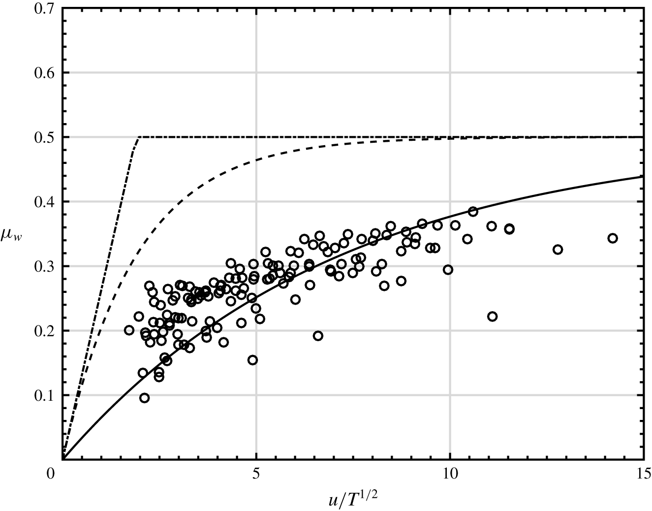
 $e_{t}\leqslant 0.6$, and indeed does not satisfactorily reproduce the effective wall friction measured in the DEM simulations (figure 6). The latter has been obtained from (3.1) and (3.2) as
 $\unicode[STIX]{x1D707}_{w}=(\tan \unicode[STIX]{x1D703}-\text{d}s/\text{d}p)((W\unicode[STIX]{x1D708}\cos \unicode[STIX]{x1D703})/2p)$ and excluding regions of the flows in which the first normal stress difference was larger than 0.3, thus limiting the scattering associated with flow anisotropy. With
 $C=0.14$ instead of 0.46, (A 2) can satisfactorily reproduce the measurements (figure 6). We emphasize that the fitted value of
 $C$ takes also into account the role of the gradients along the spanwise direction that we neglect in our approximate unidimensional treatment of the flows.
Measured (circles) effective wall friction coefficient as a function of the scaled  $x$-velocity in the DEM simulations of steady, confined incline flows at different widths and angles of inclination. Also shown are the predictions of Jenkins (Reference Jenkins1992) ((A 1), dot-dashed line) and Louge (Reference Louge1994) ((A 2) with
 $C=0.46$, dashed line), and the present suggestion ((A 2) with
 $C=0.14$, solid line).

Appendix B. Normal stress differences
Equations (3.1) and (3.2) assume that the normal stresses are isotropic and equal to the pressure. Actually, anisotropy in the stress tensor is typical of granular flows, even in steady, homogeneous conditions (Saha & Alam Reference Saha and Alam2016). In dilute flows, anisotropy in the velocity fluctuations is pronounced because of the long distances travelled between collisions and the resulting changes in momentum between the flow and normal directions (Jenkins & Richman Reference Jenkins and Richman1988). In dense flows, it has more to do with the difference between collisions in the plane and out of the plane of shearing.
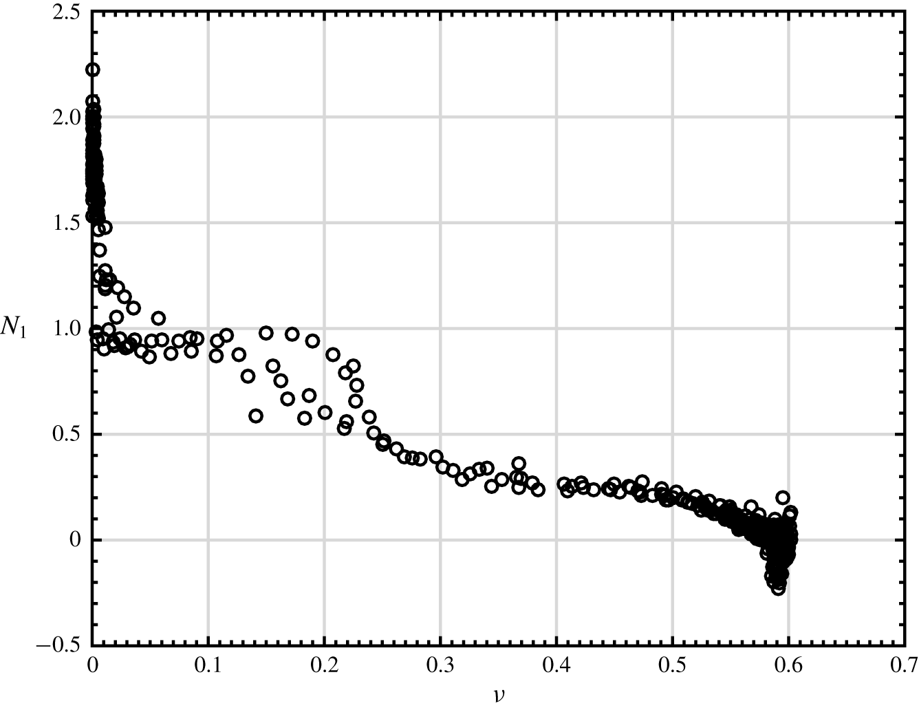
Measured (circles) first normal stress difference as a function of solid volume fraction in the DEM simulations of steady, confined incline flows at different widths, mass hold-ups and angles of inclination.

Figure 7 depicts the relation between the first normal stress difference  $N_{1}$, that is the difference between the normal stress in the
 $x$-direction and that in the
 $z$-direction divided by the pressure, and the solid volume fraction measured in DEM simulations (author’s unpublished observations). The measurements were taken at different widths, mass hold-ups and angles of inclinations. In particular, for
 ${\mathcal{M}}=25$,
 $W=30$ and
 $\unicode[STIX]{x1D703}=24^{\circ }$,
 $25^{\circ }$,
 $28^{\circ }$ and
 $30^{\circ }$; and for
 ${\mathcal{M}}=37$,
 $W=20$ and
 $\unicode[STIX]{x1D703}=30^{\circ }$,
 $35^{\circ }$,
 $40^{\circ }$ and
 $45^{\circ }$. The flows are highly anisotropic, especially in the dilute region at the top, i.e. where
 $\unicode[STIX]{x1D708}<0.2$. There, the value of
 $N_{1}$ is much larger than what measured in DEM simulations of steady, homogeneous shearing of frictionless spheres (Saha & Alam Reference Saha and Alam2016). The first normal stress difference decreases with increasing volume fraction, and can even change sign in the erodible bed, as first observed in dense, simple shear flows of disks (Alam & Luding Reference Alam and Luding2003). The EKT described in the present paper is a linear theory that does not account for the anisotropy in the particle velocity distribution and might, therefore, fail in the dilute region. It is possible to include nonlinear terms in EKT (Berzi & Jenkins Reference Berzi and Jenkins2018), but this would complicate things further, and make the present analysis less transparent.