1. Introduction
The development of intelligent transportation systems has increased the demand for active management and control of traffic flow. With the widespread deployment of universal ship automatic identification systems (AIS), there is a surge in data collection of vessel navigation information. Given such large and comprehensive datasets, extracting spatio-temporal patterns in an effective way for reliable prediction of vessel traffic flows is gaining popularity (Liang et al., Reference Liang, Liu, Zhan, Li, Zhu and Wang2022). Water transport constitutes and promotes global trade, and plays an indispensable role in the economic development of coastal or inland areas (Li et al., Reference Li, Yang and Xing2023a; Zhang et al., Reference Zhang, Gao, Xu, Tang and Guo2022). Accurate predictions of vessel flow can provide insights into traffic patterns, allowing managers to make quick and reliable decisions on waterway management and scheduling optimisation. Therefore, establishing an efficient and precise model for vessel traffic flows is a crucial step to the new era with high-quality water transportation and high-level management.
As a typical inland waterway, the Subei Canal is one of the busiest channels in the Chinese inland river system (Zhang et al., Reference Zhang, Xu, Mao, Guo, Tang and Yin2023a). Spanning 404 kilometres in northern Jiangsu Province, it forms a complex transportation network connected to the Yangtze River and numerous tributaries. Eleven multi-channel ship locks are designed to balance the water level difference along the waterway. The daily throughput of a single lock can reach 300–400, resulting in an annual cargo volume exceeding 300 million tonnes and more than 800,000 cargo ships passing through the canal each year. In contrast, according to the research by Ji et al. (Reference Ji, Zhang, Yu and Kang2021), the traffic volume of ships passing through the two locks of the Yangtze River varies between 20 and 100 per day, while ship volume involved in the Austrian River lock system (Prandtstetter et al., Reference Prandtstetter, Ritzinger, Schmidt, Ruthmair, Ochoa and Chicano2015) ranges from 40 to 100. Under these conditions, these cascaded locks serve as critical nodes in the network, while large numbers of vessels queue up and accumulate. Due to the instability of traffic flow and the short distance between locks, increased traffic flows at one lock can lead to congestion, not only affecting itself but also extending waiting times for ships at adjacent locks. Therefore, the huge transportation demand makes it crucial to carry out accurate ship flow predictions on the Subei Canal. More importantly, the interaction among locks needs to be considered when designing a forecasting model, i.e. predictions of traffic flows in one lock should be aware of the traffic flows in other locks.
The emergency of massive data and associated data-mining techniques over the past decades has prompted a transition from simple statistical methods to deep-learning approaches in traffic-flow prediction (Liu et al., Reference Liu, Rasouli, Wong, Feng and Huang2024b). As a brief recap, the statistical methods usually predict the future traffic flows based on historical data with some unrealistic assumptions (e.g. Cao et al., Reference Cao, Wu, Zhang, Wu, Cui and Chang2024). Machine learning based methods excel at recognising intricate patterns in data (Fang et al., Reference Fang, Chen, Hwang, Chang and Chang2024), which improves their performance in predicting traffic flows. However, exhaustive feature engineering requires significant effort and takes a substantial amount of time. Deep learning circumvents the cumbersome process of manual feature engineering by automatically extracting features within the network. Most recently, the graph neural networks (GNNs) have been introduced as powerful tools to handle graphical data. They can capture the dependencies within graphs through message passing between nodes (Zhou et al., Reference Zhou, Cui, Hu, Zhang, Yang, Liu, Wang, Li and Sun2020). The GNN-based approaches have been proved that they are exceptionally appropriated and extensively useful in the realm of traffic prediction (e.g. Jiang and Luo, Reference Jiang and Luo2022). Inspired by the success of convolutional neural networks (CNNs) on structural images, the graph convolutional network (GCN) has been developed to enable learning on data with non-Euclidean distance. It has gained great popularity in traffic prediction (Yu et al., Reference Yu, Lee and Sohn2020) due to its ability to capture the topological structure of transportation networks, thereby enhancing prediction accuracy (Yu et al., Reference Yu, Lee and Sohn2020; Liu et al., Reference Liu, Rasouli, Wong, Feng and Huang2024b). Generally, traffic prediction presents challenges since its intricate spatial and temporal relationships (Seng et al., Reference Seng, Lv, Liang, Shi and Fang2021; Zhao et al., Reference Zhao, Song, Zhang, Liu, Wang, Lin, Deng and Li2020). In road traffic system, traffic flow can be consequently perceived as a graph signal evolving over time (Chai et al., Reference Chai, Wang, Yang, BanaeiKashani, Hoel, Guting, Tamassia and Xiong2018). By harnessing spatial features derived from the topological graph, GCNs possess the ability to forecast future traffic conditions of a given node, including parameters such as speed, flow and density (Xu et al., Reference Xu, Huang, Song and Gong2024; Fang et al., Reference Fang, Chen, Hwang, Chang and Chang2024; Cao et al., Reference Cao, Wu, Zhang, Wu, Cui and Chang2024; Guo et al., Reference Guo, Hu, Qian, Sun, Gao and Yin2022). GCNs achieve this by capturing the traffic dynamics existing in both the historical traffic features of the target node itself and that of its neighbouring nodes (Jiang and Luo, Reference Jiang and Luo2022). Representative studies include the temporal graph convolutional network (T-GCN), which combines GCN with a Gated Recurrent Unit (GRU) to simultaneously capture both spatial and temporal features (Zhao et al., Reference Zhao, Song, Zhang, Liu, Wang, Lin, Deng and Li2020), the TC-GCN model incorporating triple cross-attention for multidimensional spatio-temporal learning (Wang et al., Reference Wang, Guo, Wu, Li and Yu2024), the spatio-temporal graph convolutional network (STGCN) for urban and highway traffic prediction (Yu et al., Reference Yu, Yin, Zhu and Lang2018), and a human-in-the-loop spatio-temporal attention-enhanced GCN for urban destination prediction (Li et al., Reference Li, Zhang, Wang, Wu and Yang2022). However, such advanced GCN-based models have rarely applied to maritime traffic forecasting. This study aims to employ the GCN-based model to predict vessel traffic flow while considering both temporal and spatial dependencies.
In terms of maritime research, Li et al. (Reference Li, Liang, Li, Yang, Du and Chen2023b) predicts the vessel flow using an improved CNN and a long short-term memory (LSTM) network. Liang et al. (Reference Liang, Liu, Zhan, Li, Zhu and Wang2022) presents a graph neural network for fine-grained vessel traffic flow prediction. Man et al. (Reference Man, Chen, Wu, Wan and Yan2024) incorporate an attention mechanism and bi-directional LSTM to capture spatio-temporal features. Li et al. (Reference Li, Pan, Liu, Sun and Zhang2024) introduce a semi-dynamic spatio-temporal GNN to forecast waterway traffic. There are few deep learning prediction studies on maritime compared with urban road transportation. For small-scale inland waterway networks, it remains relatively limited to consider spatio-temporal dependence. Referring to advanced GCN-based methods in road traffic and extending them to inland water transportation, this study adopts a multi-graph convolutional network following Liu et al. (Reference Liu, Chen, Wu, Zhen, Li and Lin2022). They propose a unified PVCGN model (physical-virtual collaboration graph network) to learn the complex ridership patterns from the graphs. It has shown satisfactory prediction results in the road traffic, whereas in maritime transportation, to the best of the authors’ knowledge, it has not been studied in inland waterway networks. However, existing studies (Jiang and Luo, Reference Jiang and Luo2022) in this field primarily offer predictions at either the regional level (Xu et al., Reference Xu, Huang, Song and Gong2024) or specific stations (He and Shin, Reference He and Shin2020). The graphs constructed mostly rely on the single graph like distance or adjacency matrix (Bikram et al., Reference Bikram, Das and Biswas2024; Yu et al., Reference Yu, Lee and Sohn2020), rarely showing the dynamic characteristics of traffic time series data within the network. It is the first time in this work that the multi-graph convolutional network combined with a GRU is applied to small-scale inland waterway network, with multilevels including regional and station-based vessel traffic flow prediction. Specifically, this method enables the prediction of traffic flow in specific areas or lock points within a given time frame, allowing the traffic management department to make proactive adjustments and prevent potential congestion. Accurate and rapid traffic flow predictions enhance the effectiveness of water transport management systems, assist in the efficient allocation of lock traffic resources, and ensure that ships navigate sections with significant water level differences more smoothly and safely, thereby improving overall operational efficiency.
In this work, to fully leverage the correlations within maritime traffic flow graphs, an advanced deep-learning based framework consisting of a multi-graph convolutional network and gated recurrent unit layer is presented. The model fills the gap in using a multi-graph convolutional network for intelligent maritime vessel traffic flow forecasting, enriching the deep-learning based applications in various water transportation networks, whether inland or ocean field. The major contributions of this paper can be summarised as follows. (1) Multiple unstructured graphs are built from the real-world data to represent spatio-temporal vessel traffic patterns at different locations. (2) A deep-learning based framework is designed to capture spatio-temporal dependencies. A multi-graph conventional network is employed to quantitatively extract such spatio-temporal characteristics among adjacent nodes in these graphs. Moreover, a gated recurrent unit layer is used to further capture the temporal characteristics of traffic through sequential traffic data. (3) Extensive experiments are conducted on two real-world traffic datasets on vessel traffic flow predictions to evaluate the model’s performance. Results show the model consistently outperforms other conventional models on both prediction tasks. The method proposed in this paper demonstrates strong generalisability and can be applied to traffic flow prediction across various regions, including oceans and inland rivers, by considering time and space correlations. This paper demonstrates the method’s effectiveness by applying it to a small-scale inland waterway transport network, where it achieved accurate prediction results. It is also adaptable for use in oceanic datasets and predictions.
The remainder of this paper is structured as follows. Section 2 details the methodology of the proposed multi-graph convolution neural network framework. The applications of the model to predict regional and station-based vessel traffic flow using two real-world datasets are illustrated in Section 3. In Section 4, extensive experiments are conducted to compare the proposed method with several benchmark models on both regional and station-based traffic flow prediction tasks. The conclusions are finally presented in Section 5.
2. Methodology
2.1. Graph convolution on unstructured graph
The GCN has been experimented broadly to the graph data in a deep-learning field. It has been proved to have great superiority in the feature extraction of non-Euclidean data with complex structures (Peng and Zhang, Reference Peng and Zhang2023). The GCN is a variant of the GNN enhancement from the spectral and spatial (vertex) domains (Fu et al., Reference Fu, Wang, Liu, Liu and Zhou2022), aiming at generalising the convolution operation and capturing each node’s structure information (Zhang et al., Reference Zhang, Zhang, Wang, Ma and Xu2023b), wherein the spatial GCN typically operates on the node level and considers the local neighbourhood structure of each node. Alternatively, the spectral GCN uses the graph’s Laplacian matrix to transform the graph data into the Fourier domain.
In this research, with regards to irregular graph data with topological structure, the waterway network can be defined as
 $G = \left( {v,{\rm{\varepsilon }}} \right)$
, where
 $v = \left\{ {{v_1}, \ldots, {v_N}} \right\}$
represents the set of nodes and
 $\varepsilon$
denotes the set of edges. A symmetric matrix
 $A \in {{\mathbb R}^{N \times N}}$
denotes the adjacency matrix of graph
 $G$
, where element
 ${a_{ij}}$
in
 $A$
is the edge weight between nodes
 $i$
and
 $j$
(Li et al., Reference Li, Pan, Liu, Sun and Zhang2024). It contains values 0 and 1, where 0 represents no link between nodes and 1 indicates the existence of a link (Liu et al., Reference Liu, Rasouli, Wong, Feng and Huang2024b).
 $\left\{ {\matrix{ {{a_{ij}} = 1,} \hfill & {{\rm{if\;}}{\varepsilon _{ij}} = 1,} \hfill \cr {{a_{ij}} = 0,} \hfill & {{\rm{otherwise}}.} \hfill \cr } } \right.$
The feature matrix
 $X = \left[ {{x_1},...,{x_N}} \right] \in {{\mathbb R}^{N \times N}}$
represents the node features. The count of vertices linked to edges can be denoted by a degree matrix
 $D$
, it can be used with the adjacency matrix to construct the graph’s Laplacian matrix.
 $\left\{ {\matrix{ {{d_{ij}} = deg\left( {{v_i}} \right),} \hfill & {{\rm{if\;}}i = j,} \hfill \cr {{d_{ij}} = 0,} \hfill & {{\rm{otherwise}},} \hfill \cr } } \right.$
where
 $deg\left( {{v_i}} \right)$
is the number of edges connected to the vertex and the undirected graph Laplacian is defined as
 $L = D - A$
with eigendecomposition
 $L = U{\rm{\Lambda }}{U^T}$
. Here,
 $U$
is an orthonormal matrix containing the Fourier basis matrix of eigenvectors of the normalised Laplacian
 $L$
and
 ${\rm{\Lambda }}$
comprises non-negative eigenvalues. The normalised Laplacian matrix is accordingly denoted as
 ${\cal{L}} = {I_n} - {D^{ - {1 \over 2}}}A{D^{ - {1 \over 2}}}$
(Peng and Zhang, Reference Peng and Zhang2023), where
 ${I_n}$
is the identity matrix with size
 $N$
.
The eigenvectors of the Laplacian matrix of a graph can be interpreted as the spectrum of the graph, enabling the Fourier transformation of the information of each node along these eigenvectors. The spectral convolution operations on graphs
 ${g_\theta }\,*\,X$
can be viewed as the product of signal
 $X$
and the filter
 ${g_\theta } = diag\left( \theta \right)$
, where
 $\theta$
parametrises the Fourier domain in
 ${\mathbb R}^N$
. The graph convolution operation in the spectral domain between signal
 $X$
and filter
 $g$
can be expressed as (Zhang et al., Reference Zhang, Zhang, Wang, Ma and Xu2023b)
 $g\left( {\cal L} \right)*X = U\left( {{U^T}g \bigodot {U^T}X} \right) = U{g_\theta }\left( {\rm{\Lambda }} \right){U^T}X$
where
 ${g_\theta }\left( {\rm{\Lambda }} \right) = diag\left( {{U^T}g} \right)$
and ⊙ denotes the Hadamard product. The signal
 $X$
undergoes transformation into the frequency domain via Fourier transform (
 ${U^T}X$
). It is then filtered by the convolution kernel
 ${g_\theta }\left( {\rm{\Lambda }} \right)$
and transformed into the original space. This spectral graph convolution is computationally expensive due to the
 ${\cal O}\left( {{N^2}} \right)$
complexity of the product with the eigenvector matrix. Moreover, computing the eigendecomposition of the Laplacian matrix becomes computationally burdensome for large graphs. To approximate the graph convolution, Defferrard et al. (Reference Defferrard, Bresson, Vandergheynst, Lee, Sugiyama, Luxburg, Guyon and Garnett2016) employed Chebyshev polynomials, thereby mitigating the issue of gradient explosion. The Chebyshev polynomials can be represented as
 ${T_n}\left( x \right) = 2x{T_{n - 1}}\left( x \right) - {T_{n - 2}}\left( x \right)$
with
 ${T_0}\left( x \right) = 1$
and
 ${T_1}\left( x \right) = x$
. Since
 ${T_n}\left( {cos\left( \theta \right)} \right) = co{s_n}\theta$
, the
 $x \in \left[ { - 1,1} \right]$
. To obtain the Laplacian matrix with eigenvalues in the range [−1,1], make
 $\hat L = {{\cal L}_{sym}} - {I_n}$
, where
 ${{\cal L}_{sym}}$
is the symmetric normalised Laplacian (
 ${{\cal L}_{sym}} = {D^{ - {1 \over 2}}}{\cal L}{D^{ - {1 \over 2}}} = {I_n} - {D^{ - {1 \over 2}}}A{D^{ - {1 \over 2}}}$
), the eigenvalue range
 $\lambda \in \left[ {0,2} \right]$
. Therefore, the operator can be denoted as (Zhou et al., Reference Zhou, Cui, Hu, Zhang, Yang, Liu, Wang, Li and Sun2020)
 $U{g_\theta }\left( {\rm{\Lambda }} \right){U^T}X = U\left( {\mathop \sum \limits_{k = 0}^K {\theta _k}{T_k}\left( {\rm{\Lambda }} \right)} \right){U^T}X = \mathop \sum \limits_{k = 0}^K {\theta _k}{T_k}\left( {{{\cal L}_{sym}} - {I_n}} \right)X$
where
 ${\theta _k}$
is the learnable parameter. Setting K to 1 and neglecting terms of second order and above, calculation can be simplified. The above formula can be approximately equal to
 ${\theta _0}{T_0}(\left( {{{\cal L}_{sym}} - {I_n}} \right)X + {\theta _1}{T_1}(\left( {{{\cal L}_{sym}} - {I_n}} \right)X$
, and it is equal to
 ${\theta _0}X + {\theta _1}(\left( {{{\cal L}_{sym}} - {I_n}} \right)X$
. Substituting into the adjacency matrix, it can be expressed as
 ${\theta _0}X - {\theta _1}{D^{ - {1 \over 2}}}A{D^{ - {1 \over 2}}}X$
. Finally, the graph convolution expression can be further developed as
 ${g_\theta }*X = \theta \left( {{I_n} + {D^{ - {1 \over 2}}}A{D^{ - {1 \over 2}}}} \right)X = \theta \left( {{{\hat D}^{ - {1 \over 2}}}\hat A{{\hat D}^{ - {1 \over 2}}}} \right)X$
where
 $\theta$
is a learnable weight matrix,
 $\hat A = A + {I_n}$
and
 ${\hat D_{ij}} = \mathop \sum \nolimits_j {{{\hat A}}_{ij}}$
(Jiang and Luo, Reference Jiang and Luo2022).
2.2. Prediction problem description of vessel traffic flow within inland waterway
The definition of traffic flow in road transportation within a given time period is the number of vehicles that pass through a spatial unit (Jiang and Luo, Reference Jiang and Luo2022). Similar to road traffic, the ship trajectory
 ${T_{raj}}$
typically comprises a sequence of location points
 ${P_j} = \left[ {Lo{n_j},La{t_j},{t_j}} \right]$
with
 $j \in \left[ {1,2, \ldots, J} \right]$
recorded by AIS devices over time. Here,
 $J$
is the number of timestamped points in
 ${T_{raj}}$
, while
 $Lo{n_j},La{t_j},{t_j}$
represent the longitude, latitude and timestamp, respectively. By aggregating trajectories, the inflows and outflows of different regions can be calculated. The maritime traffic network can be modelled as a set of undirected graphs
 $\left( {{G_i} = \left[ {{{\cal G}_d},{{\cal G}_s},{{\cal G}_{i}}} \right] = \left( {{v_i},{\varepsilon _i}} \right),i \in \left( {d,s,i} \right)} \right)$
according to topological structure (
 ${{\cal G}_d})$
, traffic pattern correlations (
 ${{\cal G}_s})$
and local interactivity (
 ${{\cal G}_i})$
. For vessel traffic flow characterised by regional inflow and outflow, nodes are denoted as
 $n$
. Based on graph theory, the distance matrix can be employed to mathematically indicate the topological relationship between different vertexes of the graph
 $G$
.
Given that at time
 $\tau$
, the traffic data recorded by sensor
 ${s_i}$
are
 $a_{si}^t$
, the data detected by
 ${s_i}$
over period of
 $\left( {\tau - m + 1} \right)\sim \tau$
are from the series
 $a_{si}^{\tau - m + 1\sim \tau }$
. Accordingly, the traffic data across all nodes collected by sensors of the maritime network can be expressed by the matrix
 ${X^{\left( {\tau - m + 1} \right)\;\sim \tau }} \in {{\mathbb R}^{N \times N}}$
(Peng and Zhang, Reference Peng and Zhang2023).
 ${X^{\left( {\tau - m + 1} \right)\sim \tau }} = \left( {\matrix{ {a_{s1}^{\left( {\tau - m + 1} \right)}} \hfill & {a_{s2}^{\left( {\tau - m + 1} \right)}} \hfill & \cdots \hfill & {a_{{\rm{s}}n}^{\left( {\tau - m + 1} \right)}} \hfill \cr {a_{s1}^{\left( {\tau - m + 2} \right)}} \hfill & {a_{s2}^{\left( {\tau - m + 2} \right)}} \hfill & \cdots \hfill & {a_{sn}^{\left( {\tau - m + 2} \right)}} \hfill \cr \hskip 9pt\cdots \hfill & \hskip 9pt\cdots \hfill & \cdots \hfill & \hskip 9pt\cdots \hfill \cr \hskip 9pt{a_{s1}^\tau } \hfill & \hskip 9pt{a_{s2}^\tau } \hfill & \cdots \hfill & \hskip 9pt{a_{sn}^\tau } \hfill \cr {} \hfill & {} \hfill & {} \hfill & {} \hfill \cr } } \right)$
For any row
 ${X^i} = \left[ {a_{s1}^i,a_{s2}^i, \ldots, a_{sn}^i} \right]$
of
 ${X^{\left( {\tau - m + 1} \right)\sim \tau }}$
, it denotes the traffic data detected by each node of the network at a given time
 $i$
, and for each column,
 $X_{sj}^{\left( {\tau - m + 1} \right)\sim \tau } = \left[ {a_{sj}^{\left( {\tau - m + 1} \right)},a_{sj}^{\left( {\tau - m + 2} \right)}, \ldots, a_{sj}^\tau } \right]$
of
 ${X^{\left( {\tau - m + 1} \right)\sim \tau }}$
means the traffic data obtained by a single node
 ${s_j}$
over period of
 $\left( {\tau - m + 1} \right)\sim \tau$
. The definition of
 ${X^{\left( {\tau - m + 1} \right)\sim \tau }}$
reflects the spatio-temporal characteristics between different locations.
Two levels of vessel traffic flow problems of the maritime network are considered, namely regional level and station-based level prediction. Regional level flow problems focus on traffic volume within spatial regions. Station-based traffic flow problems pertain to the volume recorded at a physical station such as a port or a lock. In the regional vessel traffic prediction task, the inflow at time interval
 $t$
(e.g. one hour) can be expressed as
 ${I^t} = \left[ {I_1^t,I_2^t, \ldots, I_n^t} \right]$
and outflow at time interval
 $t$
can be expressed as
 ${O^t} = \left[ {O_1^t,O_2^t, \ldots, O_n^t} \right]$
. However, for stations, the ship passage information is recorded by serial locks and the traffic flow of
 $n$
nodes can be counted at fixed intervals, denoted as
 ${Q^t} = \left[ {Q_1^t,Q_2^t, \ldots, Q_n^t} \right]$
. Suppose the current time is
 $\tau$
. Given historical vessel traffic flow data and the corresponding network diagrams spanning
 $m$
time periods in the past, the learning of the traffic prediction model
 ${\cal F}$
to forecast the traffic status of regions and stations for
 $T$
time steps in the future can be summarised as (Seng et al., Reference Seng, Lv, Liang, Shi and Fang2021)
 $\eqalign{ & {\widehat {({I^t},{O^t})}}^{\tau + 1},...,{\widehat {({I^t}\hat, {O^t})}}^{\tau + T} = F({({I^t},{O^t})^{\tau - m + 1}},...,\left( {{I^t},{O^t}{)^\tau };{G_i}} \right) \cr & {({{\hat Q}^t})^{\tau + 1}},...,{({{\hat Q}^t})^{\tau + T}} = F({({Q^t})^{\tau - m + 1}},...,\left( {{Q^t}{)^\tau };{G_i}} \right) \cr}$
2.3. Unstructured graphs construction
Different graph structures are used to model the traffic prediction problem, depending on prediction tasks and the characteristics of the available datasets (Jiang and Luo, Reference Jiang and Luo2022). Employing multiple graphs to depict spatial relationships among various regions or stations extends beyond merely considering physical distances. It encompasses capturing historical records and temporal relationships among different nodes. By constructing these multiple graphs to encapsulate spatio-temporal relationships and applying convolutional layer to integrate them, the vessel traffic flow prediction reliability can be significantly enhanced.
Distance graph
. The topological structure
 ${{\cal G}_d}$
of the maritime network is directly built based on the distance between nodes. The edge weight is the distance between two regions or stations. The elements in the distance graph are calculated as follows, where
 $dist\left( {i,j} \right)$
is the geographically distance between nodes
 $i$
and
 $j$
:
 ${A_d}\left( {i,j} \right) = \left\{ {\matrix{ {dist\left( {i,j} \right),} \hfill & {{\rm{if\;}}i \ne j,} \hfill \cr {{a_{ij}} = 0,} \hfill & {{\rm{if\;}}i = j.} \hfill \cr } } \right.$
Similarity graph
. The historical inflow and outflow traffic data of each region, or that of stations within fixed time intervals (e.g. one hour), can be aggregated. Afterwards, the correlations between two nodes can be computed. The popular Pearson coefficient (PCC) based on hourly traffic time series is adopted to quantify the similarity between regions or stations. The similarity graph
 ${{\cal G}_s}$
can be expressed as
 ${A_s}\left( {i,j} \right) = \left\{ {\matrix{ {PCC\left( {{h_i},{h_j}} \right),} \hfill & {{\rm{if\;}}i \ne j,} \hfill \cr {{a_{ij}} = 0,} \hfill & {{\rm{if\;}}i = j.} \hfill \cr } } \right.$
Interaction graph
. Bidirectional flow yields a substantial volume of spatial information regarding the movement of ships between various regions. An interaction graph is thereby constructed to show whether two regions have frequently interacted with each other based on the historical records. The number of shipping records between
 $i$
and
 $j$
is represented as
 ${d_{i,j}}$
, and the interaction graph
 ${{\cal G}_i}$
can be built as
 ${A_i}\left( {i,j} \right) = \left( {\matrix{ {{d_{1,1}}} \hfill & {{d_{1,2}}} \hfill & \cdots \hfill & {{d_{1,n}}} \hfill \cr {{d_{2,1}}} \hfill & {{d_{2,2}}} \hfill & \cdots \hfill & {{d_{2,n}}} \hfill \cr \cdots \hfill & \cdots \hfill & \cdots \hfill & \cdots \hfill \cr {{d_{n,1}}} \hfill & {{d_{n,2}}} \hfill & \cdots \hfill & {{d_{n,n}}} \hfill \cr } } \right)$
2.4. Prediction of Inland waterway vessel traffic flow
Each constructed graph undergoes processing by GCN. Subsequently, three feature matrices are fused, with the weighting of each matrix adjusted using learnable parameters
 ${W_d}$
,
 ${W_s}$
and
 ${W_i}$
. Normalisation of the parameter matrix is achieved through the application of the softmax operation (Chai et al., Reference Chai, Wang, Yang, BanaeiKashani, Hoel, Guting, Tamassia and Xiong2018).
 $\matrix{ {} \hfill & {W{{\rm{'}}\!\!_d},W{{\rm{'}}\!\!_s},W{{\rm{'}}\!\!_i} = softmax\left( {{W_d},{W_s},{W_i}} \right)} \hfill \cr {} \hfill & {G_{fusion}^\tau = W{{\rm{'}}_d} \ \bigodot {f_d}\left( {{X^\tau },{A_d}} \right) + W{{\rm{'}}_s} \,\bigodot {f_s}\left( {{X^\tau },{A_s}} \right) + W{{\rm{'}}_i} \,\bigodot {f_i}\left( {{X^\tau },{A_i}} \right)} \hfill \cr }$
where
 ${f_j}\left( {{X^\tau },{A_j}} \right) = \theta \left( {{{\hat D}^{ - {1 \over 2}}}{{\hat A}_j}{{\hat D}^{ - {1 \over 2}}}} \right){X^\tau }$
,
 $j \in \left( {d,s,i} \right)$
, represents the graph fusion result, which will be used in the graph convolution process. Multiple graphs are fused by the weight matrices as
 $G_{fusion}^\tau$
. Here,
 $\,\bigodot$
is an element-wise multiplication operator.
Furthermore, the GRU is employed for temporal feature learning. Compared with LSTM, GRU contains fewer parameters, resulting in shorter training times while maintaining comparable performance. The GRU retrieves the traffic status at time
 $\tau$
by leveraging the hidden state at time
 $\tau - 1$
along with the multi-graph convolution result. Specifically, the update gate
 ${Z_\tau }$
plays a crucial role in determining how the current hidden state,
 ${h_\tau }$
, is updated by the candidate hidden state,
 ${\tilde h_\tau }$
, which incorporates information from the current time step. The reset gate,
 ${R_\tau }$
, regulates how the hidden state,
 ${h_{\tau - 1}}$
, from the previous time step influences the candidate hidden state for the current time step. The detailed expressions are as follows (Zhao et al., Reference Zhao, Song, Zhang, Liu, Wang, Lin, Deng and Li2020):
 $\matrix{ {{Z_\tau }} & \hskip-22pt{ = \sigma \left( {{W_z} \cdot \left[ {{h_{\tau - 1}},{x_\tau }} \right] + {b_z}} \right) = \sigma \left( {{W_{zh}}{h_{\tau - 1}} + {W_{zx}}{x_\tau } + {b_z}} \right)} \cr {{R_\tau }} & \hskip-22pt{ = \sigma \left( {{W_r} \cdot \left[ {{h_{\tau - 1}},{x_\tau }} \right] + {b_r}} \right) = \sigma \left( {{W_{rh}}{h_{\tau - 1}} + {W_{rx}}{x_\tau } + {b_r}} \right)} \cr {{{\tilde h}_\tau }} & \hskip-9pt{ = {\rm{tanh}}\left( {{W_h} \cdot \left[ {{R_\tau } \,\bigodot {h_{\tau - 1}},{x_\tau }} \right] + {b_h}} \right)} \,\,\,\,\,\,\,\,\,\,\,\,\,\,\,\,\,\,\,\,\,\,\,\,\,\,\,\,\,\,\,\,\,\,\,\,\,\,\,\,\,\,\,\,\,\,\,\,\,\,\,\,\,\cr {} & \hskip-15pt{ = {\rm{tanh}}\left( {{W_{hh}}\left( {{R_\tau } \,\bigodot {h_{\tau - 1}}} \right) + {W_{hx}}{x_\tau } + {b_h}} \right)} \,\,\,\,\,\,\,\,\,\,\,\,\,\,\,\,\,\,\,\,\,\,\,\,\,\,\,\,\,\,\,\,\,\,\,\,\,\cr {{h_\tau }} & \hskip-6pt{ = {h_{\tau - 1}} \,\bigodot {Z_\tau } + {{\tilde h}_\tau } \,\bigodot \left( {1 - {Z_\tau }} \right)} \,\,\,\,\,\,\,\,\,\,\,\,\,\,\,\,\,\,\,\,\,\,\,\,\,\,\,\,\,\,\,\,\,\,\,\,\,\,\,\,\,\,\,\,\,\,\,\,\,\,\,\,\,\,\,\,\,\,\,\,\,\,\,\,\,\,\,\cr }$
In this vessel traffic prediction task, GRU captures temporal dependencies from sequential observations. The network takes the traffic volume at time
 $\tau$
,
 ${x_\tau }$
and the hidden state at time
 $\tau - 1$
,
 ${h_{\tau - 1}},$
as model input. It generates the output
 ${h_\tau }$
using the update gate, reset gate and current memory content denoted by
 $_\tau$
,
 ${R_\tau }$
and
 ${\tilde h_\tau }$
. The architecture of the proposed deep-learning framework consisting of a multi-graph convolution network and GRU for multi-step prediction of vessel traffic flow within inland waterway network is shown in Figure 1. After preprocessing, traffic statistics are aggregated into one-hour intervals, different graphs of regions or stations are constructed and further fed into the graphic convolutional layers. The framework adopts an encoder and decoder structure, both of which contain two GRU layers aiming to capture temporal information about historical traffic sequence and forecast traffic of corresponding nodes for multiple time steps. The graphic convolutional network and the gated recurrent unit network are jointly trained based on two split real-world traffic datasets. To evaluate the prediction results on the test dataset, the mean absolute error (MAE), mean absolute percentage error (MAPE) as well as normalised root mean square error (RMSE) are employed, with a smaller value indicating higher prediction accuracy.
Overview of the multi-graphic convolution network for regional and station-based vessel traffic flow prediction within inland waterway networks.

3. Case study
3.1. Study area and dataset
The surge in heavy traffic demand has exerted increasing pressure on the inland waterway. To predict the vessel traffic flow of regions or stations, multi-source datasets were gathered. Specifically, for regional prediction, a total of 23,350,335 AIS records in the study area were collected from the Jiangsu Provincial Department of Transportation Port and Shipping Development Center, covering the following spatial and temporal ranges: longitude from
 ${117.5^ \circ }$
to
 ${121^ \circ }$
, latitude from
 ${32.2^ \circ }$
to
 ${34.6^ \circ }$
. For station-based prediction, ship passage records were collected from ten locks within the study area. These two datasets cover the period from 00:00:00 on November 26, 2023 to 24:00:00 on December 25, 2023. In this work, 80
 ${\rm{\% }}$
of the traffic data is selected as the training set, while the remaining 20
 ${\rm{\% }}$
is used for testing.
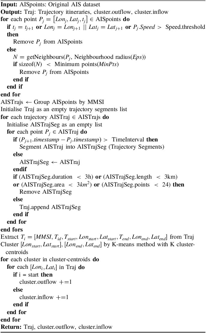
For AIS dataset processing and trajectories extraction, the obtained point distribution diagrams before and after cleaning are illustrated in Figure 2, and several cleaning measures (Zhao et al., Reference Zhao, Shi and Yang2018) were taken. (1) Identify and eliminate duplicate entries based on key identifiers such as timestamp, vessel name and location coordinates. (2) Filter out trajectory points where the speed exceeds 14 knots to consider the canal navigation characteristics. (3) Trajectory points outside the waterway and outliers are removed in the geographic domain. (4) Implement a 24-hours interval threshold segmentation on the trajectories, removing trajectories with less than 24 points. (5) Exclude trajectories with duration less than 3 hours. (6) Filter out trajectories where the distance computed between start and end points, together with the cumulative distance between adjacent points is less than 3 kilometres. (7) Remove trajectories whose maximum area, formed by points within the trajectory range, is less than 1 square kilometre. In addition, the density based spatial clustering of applications with noise algorithm (DBSCAN) (Fujino and Claramunt, Reference Fujino and Claramunt2023) was also adopted to distinguish undesired outliers. Exhaustive experiments were conducted to empirically determine the suitable parameter values of
 $Eps$
and
 $MinPits$
. As
 $Eps$
increases, the retained feature points ratio initially rises and then stabilises gradually. In contrast, the proportion of the remaining feature points changes slowly with the increase of
 $MinPits$
. The optimal parameters of
 $Eps$
and
 $MinPits$
are empirically chosen as 0.18 and 3 based on the experimental results.
Comparison of AIS dataset before and after cleaning.

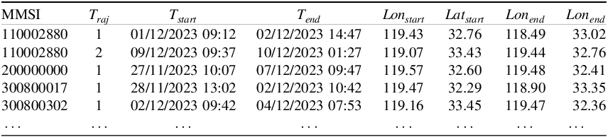
After cleaning and segmenting the trajectory data, the starting and ending points of each trajectory, together with their corresponding temporal and spatial information, are extracted as in Table 1, that is,
 ${T_i} = \left[ {MMSI,{T_{id}},{T_{start}},o{n_{start}},La{t_{start}},{T_{end}},Lo{n_{{\rm{e}}nd}},La{t_{end}}} \right]$
. This implies that a vessel identified by a specific Maritime Mobile Service Identity (MMSI) departs from position (
 $Lo{n_{start}},La{t_{start}}$
) and time
 ${T_{start}}$
corresponding to the beginning of its
 ${T_{id}}$
voyage, and arrives at the destination (
 $Lo{n_{end}},La{t_{end}})$
at time
 ${T_{end}}$
. The dataset extracted contains a total of 30,294 vessel trajectories within one month because of the high repeatability of round trips in inland waterways.
Trajectory information extracted from processed AIS dataset.

In contrast to the extensive voyages undertaken by vessels navigating in the ocean, inland waterway vessels primarily cater to the demand for short-distance transportation. Navigation within an inland waterway network exhibits a repetitive journey pattern, characterised by relatively short voyage duration and distance. Analysis of ship trajectory data, as illustrated in Figure 3, reveals a median voyage duration of 24.5 hours and a median travel distance of 45.0 kilometres. Hence, the one-month AIS ship trajectory data collected in this study is sufficient to elucidate the behavioural characteristics of inland vessel movements. It effectively reveals the navigation patterns and traffic attributes distinctive to inland waterways. To gain deeper insights into the distribution of trips, the location information of both the starting and ending points are clustered. The K-means method is employed, and selects K as 16 based on the Silhouette score and Davies-Bouldin index, as shown in Figure 4. The overall process on AIS dataset for regional prediction is illustrated in Algorithm 1 (Lei et al., Reference Lei, Chu, Wu, Liu, Luo, He and Liu2024).
Statistics on ship characteristics including voyage duration and distance.

Clusters of the vessel traffic flow within inland waterway network by K-means clustering method.

Processing AIS Dataset for Regional Prediction Task.

As ships pass through these locks along the Subei Canal, detailed operational information, including scheduling time and passing time, is recorded. Based on these records, vessel traffic flow at the 10 lock stations can be aggregated at 1-h intervals. Each ship passage record is represented as
 ${R_i} = \left[ {Ship,Lock,Length,Width,Tons,Tim{e_{Schedule}},Tim{e_{Pass}}} \right]$
. For a more detailed observation of traffic from the station perspective, the ship passage data are shown in Table 2. Specifically, length, width and tonnes represent the ship’s dimensions and weight. Additionally, Schedule-Time is the time when the operator specifies the scheduling plan after the ship arrives at the lock. Pass-Time is the time of confirmation that the ship leaves the lock after the lock operation. Furthermore, ten ship lock locations identified from ZZ01 to ZZ10 along the Subei Canal are shown in Figure 5. It can be observed that the distances between the locks vary and research (Ji et al., Reference Ji, Zhang, Zhang, Yu and Van Woensel2022) has demonstrated inter-dependencies among sequential locks, particularly when lock throughput is low and the distance between consecutive locks is short, resulting in high traffic flow. Based on the aggregated 1-hour traffic flow data, two types of prediction tasks are constructed. At the regional level, traffic flow is represented by a two-dimensional vector consisting of inflow and outflow, capturing bidirectional vessel movements within a canal segment. At the station level, traffic flow is defined as a one-dimensional variable representing the number of vessels passing through an individual lock within each hour. These hourly flow series serve as the input features for the corresponding regional- and station-based prediction models.
Example of records of ships passage information.

Locks on the Subei Canal within the study area.

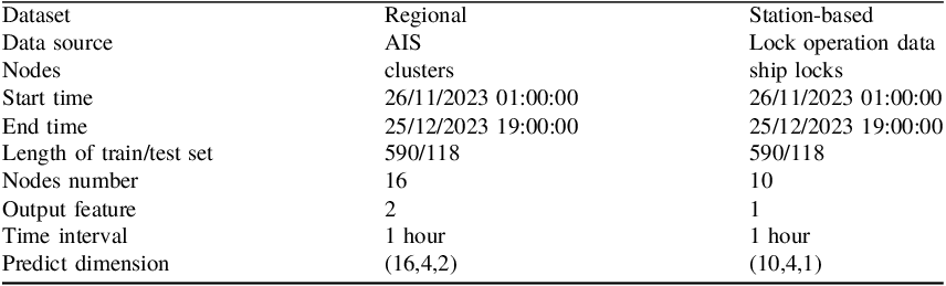
To forecast regional- and station-based vessel traffic flow, data from multiple sources are leveraged. The datasets used for these two levels of prediction are summarised in Table 3. The analysis considers 16 clusters and 10 locks as nodes, with the input and output features numbering 2 and 1, respectively. The prediction methodology involves using historical traffic data from the previous four hours to predict the traffic for the next four hours. The prediction from two perspectives is based on the small scale and management characteristics of the inland waterway network. Since multiple locks within a single city are usually governed by one administrative authority, regional predictions assist city management in overall flow control and timely interventions. Meanwhile, station-based predictions enable individual lock management units to forecast traffic demand and deploy scheduling plans in advance.
The properties of the two datasets.

3.2. Regional vessel traffic flow prediction based on clusters
Traffic data are extracted from the historical trajectories, which record the inflow and outflow of 16 nodes in hourly time slices. For instance, the outflow and inflow of cluster 7 during the study period are shown in Figure 6. Although the Augmented Dickey–Fuller test determined that both the time series are statistically stationary, their high volatility and lack of clear trends or seasonality make accurate prediction challenging, which complicate and render difficult the use of conventional time series forecasting methods.
Sequential traffic inflow and outflow data of cluster 7.

The hyperparameters of the model are categorised into structural parameters and training parameters. Since hyperparameters significantly influence the performance of a deep learning model, various network configurations are compared and the optimal model parameters are selected based on predictive performance. In this study, the input sequence length and the output sequence length are both designed as 4 to realise the multi-step prediction. Taking the training set as an example, the inflow and outflow data from 01:00 to 04:00 on November 26, 2023, are used to predict the flow values for the interval of 05:00–08:00. Based on the concept of graphs, the distance graph, similarity graph and interaction record graph are constructed. Both the encoder and decoder used in the experiment consist of two GRU layers. The number of units in the hidden layer is set to 64 considering both calculation efficiency and prediction accuracy after numerous attempts. The input and output dimensions are both set as 2 including the indicators of inflow and outflow values. The optimisation algorithm used is ADAM with a learning rate set to 0.1
 ${\rm{\% }}$
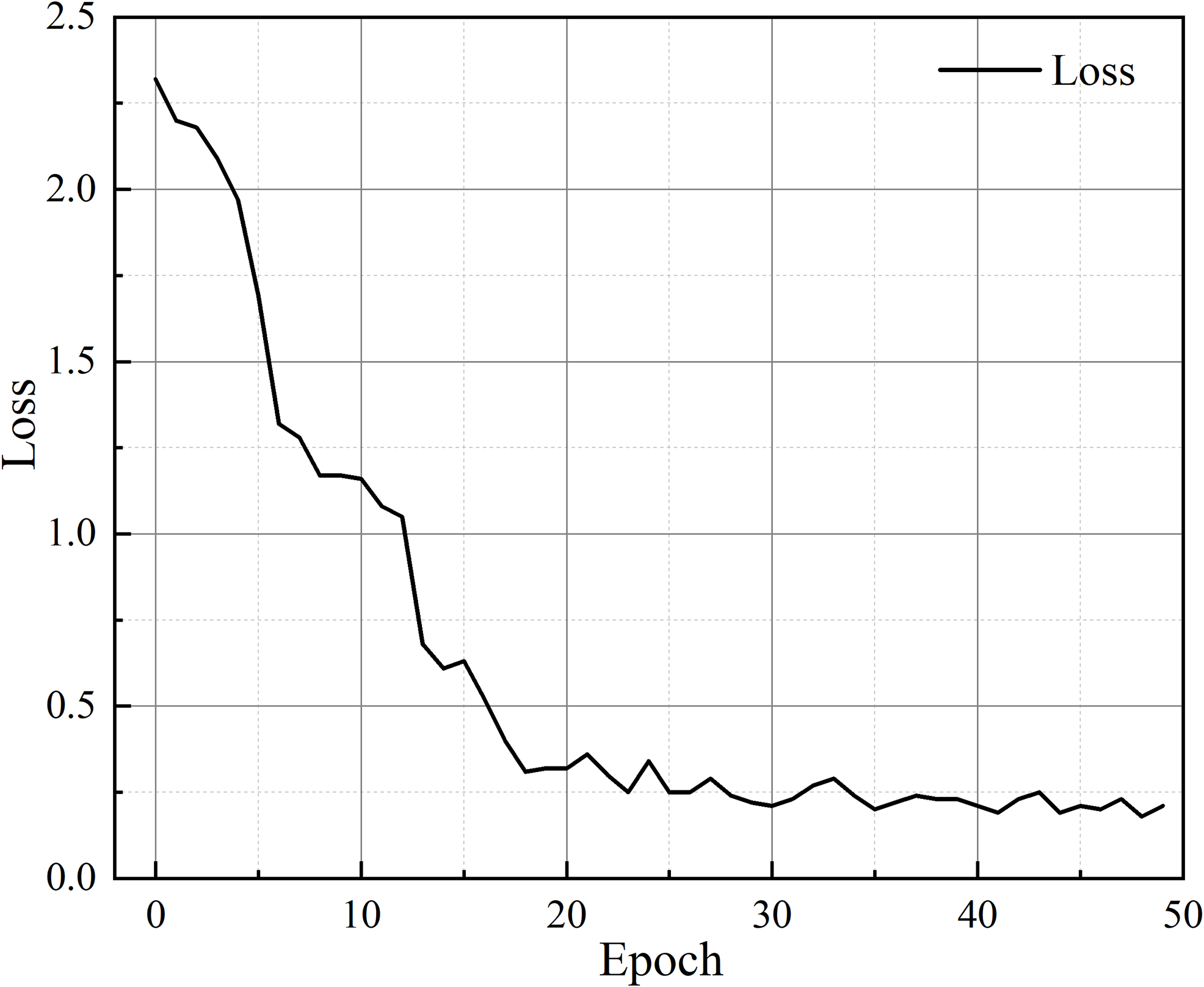
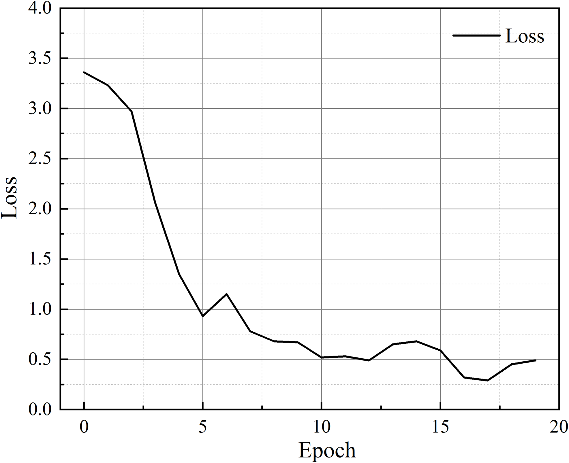
. After 50 iterations, the model has converged and achieved good results. Figure 7 presents the error and convergence curve of the model as a line graph, reflecting its performance during the training period.
Loss in the training set of regional vessel traffic flow prediction.

As illustrated in the figure, the x-axis represents the number of trained epochs and the y-axis reflects the loss observed during the experiment. The error gradually decreases as the epochs increase. An early stop strategy is incorporated, whereby the algorithm terminates training if the performance is no longer improving. The predicted inflow and outflow of 16 clusters show good consistency with the true values, indicating the excellent performance of the model. For example, Figures 8 and 9 present the training results of inflow and outflow predictions for cluster 4 and cluster 9, respectively. By carefully examining the inflow curve of cluster 4 or outflow curve of cluster 9, the model has demonstrated its superiority in predicting multiple indicators of inflow and outflow, as well as in multi-time step prediction. The MAE, MAPE and RMSE of the whole training set are 1.36, 10.40 and 2.84, respectively. It demonstrates that the proposed multi-graph convolutional network is effective for spatio-temporal regional level vessel traffic flow prediction.
Regional vessel traffic inflow predicted and true values of train set (taking cluster 4 as an example).

Regional vessel traffic outflow predicted and true values of train set (taking cluster 9 as an example).

The trained model is first restored using the saved hyperparameters and model settings, and then applied to the test set. The batch size is set to 8, covering a continuous period of 118 hours. The evaluation results indicate that the proposed model achieves an MAE of 0.16, an MAPE of 6.68 and an RMSE of 0.26. The comparison between the predicted and true values, corresponding to inflow and outflow scenarios of the whole test set, is visualised in Figures 10 and 11. It can be observed that the scatter of true and predicted values almost coincides at each time, showing particularly small errors. From a cluster-wise perspective, the model performs consistently well across clusters with heterogeneous traffic characteristics, including high-flow clusters (e.g. clusters 1, 2, 8 and 12) as well as low-flow or intermittent clusters (e.g. clusters 7 and 14). In particular, for cluster 7, where the early-stage inflow remains nearly constant at zero for an extended period, the model still successfully detects and predicts traffic variations in later periods. This behaviour suggests that the proposed model does not rely solely on the historical temporal patterns of an individual cluster, but instead leverages spatial dependencies among adjacent clusters to infer potential traffic changes. The consistency observed between inflow and outflow predictions further confirms the robustness of the model under different traffic directions. Despite the directional differences in traffic dynamics, the model maintains stable prediction accuracy, demonstrating its ability to learn directional spatial interactions and temporal evolution simultaneously.
Regional vessel traffic inflow predicted and true values of the test set.

Regional vessel traffic outflow predicted and true values of the test set.

To better illustrate the correlation between real and predicted values, the inflow of cluster 1 and the outflow of cluster 12 in Figure 12 are taken as examples to show the density distribution of the points. The results reveal that most points are concentrated near the 1-1 line, indicating a strong positive correlation. The coefficient of determination (
 ${R^2}$
) exceeds 0.9, which demonstrates the model’s excellent prediction accuracy, with the predicted values closely matching the true values. This high
 ${R^2}$
value underscores the model’s ability to accurately capture and predict the traffic patterns.
Scatter density of clusters’ predicted and true values.

3.3. Station-based vessel traffic flow prediction based on locks
Section 3.2 primarily emphasises the inflow and outflow of ships in the cluster-based regions. However, acquiring AIS data can be challenging due to varying ownership, and extracting and computing trajectories requires extensive pre-processing, although AIS data offer a broad, forward-looking perspective on large-scale flow changes across the entire region. This section, however, focuses on the time information recorded by ships when they pass through locks. The records make it easier to identify vessel traffic demand and operational pressure on individual locks over short-term horizons. It delves into more detailed analysis and considers how the flow changes at a specific ship lock are influenced by other ship locks. For the 10 locks in the study area, taking ZZ01 and ZZ02 close to the Yangtze River as examples, the true values of the vessel traffic flow is shown in Figure 13. It shows that the vessel traffic flow lacks a fixed pattern or regularity, exhibiting irregular fluctuations and trends over time. Consequently, it remains difficult for lock operators to estimate short-term passage demand solely based on temporal information.
Sequential traffic flow data of the ZZ01 and ZZ02 stations.

During the training phase, the distance graph and similarity graph are built and fed into the graph convolution layer to perform the convolution operation, and to extract the spatio-temporal characteristics among adjacent nodes. The historical four hours traffic data are sequentially fed into the GRU layers with encoder, and the output hidden states are fed into a fully connected layer to predict the next four hours of traffic flow at each station. Figure 14 illustrates the loss during the training period, revealing the error decreases as the number of iterations increases.
Loss in the training set of station-based vessel traffic flow prediction.

To further demonstrate the correlation between real and predicted values, the scatter density on the training set is presented in Figure 15. The scatter density plots show most points clustered near the 1-1 line. Among them, the value of
 ${R^2}$
exceeds 0.9, which demonstrates the model’s excellent prediction accuracy, with predicted values closely matching the true observations. As depicted in Figure 15, the model presented in this work shows excellent performance on station-based vessel traffic flow prediction. By constructing several graphs, both temporal and spatial characteristics can be effectively captured, enabling accurate predictions. The MAE, MAPE and RMSE of the training set are 0.57, 5.74 and 1.00, respectively. After saving the hyperparameters and model settings of the trained model, they were loaded and applied to the test set for evaluation. The batch size of the test set is 8, covering 118 hours. The comparison between predicted indicators and the true values of the entire test set can be visualised in Figure 16. The evaluation result indicates an MAE of 0.38, an MAPE of 4.59 and an RMSE of 0.78.
Scatter density of predicted and true values of station-based traffic flow of the training set.

Comparison on station-based traffic flow predicted and true values of the test set.

4. Discussion
The fusion of graphs realises the capture of spatio-temporal characteristics, further combined with the GRU layers to recognise the temporal independence, enhancing vessel traffic flow prediction accuracy. It is widely recognised that the traffic flow within the inland waterway network is closely related to the locations of different segments (Man et al., Reference Man, Chen, Wu, Wan and Yan2024; Li et al., Reference Li, Pan, Liu, Sun and Zhang2024), while the special navigation behaviour in inland waterway also affect changes in vessel traffic flow. By observing the real traffic time series of the locks, it can be found that the hourly average flow rate between the southern ship locks ZZ01 to ZZ03 ranges from 13 to 15, whereas the northern locks ZZ09 and ZZ10 record values of less than 5. ZZ01, serving as the linkage between the Yangtze River and the canal, has heavy traffic demand. ZZ03, however, acts as an intersection for multiple water transportation systems, including the Huaihe River, Lixia River and the Grand Canal upstream. This convergence attracts a multitude of ships, rendering ZZ03 a prominent hub for waterborne trade. It stands out as the busiest ship lock on the canal, boasting the highest throughput. From the time perspective, vessel traffic at nodes on inland waterways exhibits a certain pattern. Since vessels on inland rivers are typically manned with only the necessary crews and no additional resource allocation. Simultaneously, the crew will opt to rest for several hours at night because the sight on inland rivers is limited, resulting in a low-peak trend in node traffic flow. The model constructed in this work realises the identification and capture of such traffic relationships in time and space dimensions, so that it can accurately forecast the traffic at each node.
Regarding the two different purposes of predictions, using data from diverse sources for ship traffic prediction across various regions and stations can complement each other, mitigating unpredictability caused by insufficient data. Since the AIS data are initially obtained as thousands of point data, it requires filtering to extract ship information and corresponding voyages, identifying each ship’s origin location and time, and conducting regional clustering based on voyage details for inter-region traffic prediction. The regional flow obtained in this way considers the dynamic information of the ship. Predicting ship flow across entire regions or multiple regions aids waterway network management. The vessel traffic flow prediction of locks, based on the recorded time data as ships passed through the locks, offers easier data access and operation. The model comprehensively considers interaction between upstream and downstream locks, enabling detailed observation of flow changes at each lock and aiding in early deployment of lock scheduling strategies.
To demonstrate the superior performance of the model, we compared it against some other conventional traffic flow prediction models. The methods are as follows.
-
1) Historical Average (HA). HA is a naive statistics method to predict future vessel traffic flow by calculating the average value of traffic flow over the previous four hours of data (Fang et al., Reference Fang, Chen, Hwang, Chang and Chang2024).
-
2) Auto-regressive integrated moving average (ARIMA). ARIMA can be used for time series analysis and forecasting combining concepts of auto-regression (AR), differencing (I) and moving average (MA) components (Seng et al., Reference Seng, Lv, Liang, Shi and Fang2021).
-
3) Random Forest (RF). RF is a machine learning method for prediction. Scikit-learn is used to implement this model. Each tree in the random forest is built using the entire dataset, and the number of trees in the forest is set to 10 (Ye et al., Reference Ye, Fang, Sun, Zhang and Xiang2022).
-
4) Long short-term memory (LSTM). This RNN-based model consists of two LSTM layers with 64 units each, using ReLU activation function. There is a dense output layer with 1 unit compiled with the Adam optimiser using mean squared error loss (Liu et al., Reference Liu, Rasouli, Wong, Feng and Huang2024a).
-
5) Graph convolution network (GCN). To delve deeper into assessing the effectiveness of multiple graphs on prediction accuracy, the GCN based on a single graph is employed to conduct the same prediction. The prediction results of single graph (i.e. distance, similarity or interaction graph) named GCND, GCNS and GCNI as well as multi-graphs fusion variants are conducted (Yang et al., Reference Yang, Li and Qi2024).
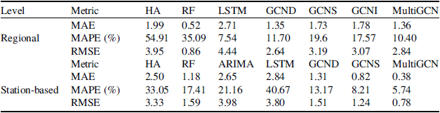
Table 4 presents a comprehensive performance comparison of the different models for vessel traffic flow prediction at both regional and station-based levels, using trajectory data extracted from AIS records and lock operation datasets. Overall, the proposed MultiGCN model consistently outperforms all benchmark methods across all evaluation metrics, including MAE, MAPE and RMSE, demonstrating its superior predictive capability under different spatial aggregation levels. Among these examined models, statistic methods such as HA and ARIMA rely on the hourly traffic flow time series data of individual nodes. The rise in traffic at interconnected nodes inevitably influences the traffic flow at this specific node in subsequent moments. However, since only its own timing is considered, this impact is overlooked. Consequently, the performance of these models falls short of expectations. Machine learning methods such as RF incorporate recent traffic data and employ more intricate prediction mechanisms. However, they tend to disregard differences between nodes, thereby impacting predictive accuracy. Similarly, LSTM-based models trained independently for each node focus on temporal dependencies but neglect spatial correlations, which are critical for traffic flow prediction in cascaded lock systems, leading to suboptimal performance.
Performance comparison for different methods on regional and station-based vessel traffic flow prediction.

In contrast, GCN-based models explicitly incorporate spatial dependencies by modelling the transportation network as a graph. The single-graph GCN variants (GCND, GCNS and GCNI) improve prediction accuracy by leveraging different types of spatial relationships, including topological distance, flow similarity and historical interaction patterns. However, each single-graph model captures only one aspect of spatial dependency, which limits its ability to fully represent the complex and heterogeneous interactions among locks. However, prediction performance varies across different graphs, wherein distance graphs depict topological relationships between nodes, and similarity and interaction graphs illustrate time series traffic flow temporal characteristics between them. For regional prediction, the multi-graphs fusion demonstrates superior performance. Among the various types of graphs used in this fusion process, it appears that the distance graph exerts the most significant influence on forecasting outcomes. In station-based prediction, compared with just considering topological distance graphs with multi-graphs fusion, the MAE of constructing multi-graphs increased by 70.99
 ${\rm{\% }}$
and the RMSE increased by 48.34
 ${\rm{\% }}$
. In contrast, the MAE of the prediction result that only builds the temporal similarity graph increased by 53.66
 ${\rm{\% }}$
and the RMSE increased by 37.10
 ${\rm{\% }}$
. This indicates that the similarity adjacency matrix updates based on the sequential traffic data between nodes can capture the spatio-temporal characteristics to a greater extent. The prediction outcomes derived from both single graph and multi-graphs fusion methodologies exhibit dynamic changes across iterations, as illustrated in Figure 17.
Model performance of single-graph and multi-graph convolution over iterations.

Combining the prediction results from the two different purposes, it becomes evident that the model proposed in this work exhibits smaller errors, particularly in refined station-level prediction results. One possible explanation for this phenomenon could lie in the processing of AIS data. During this process, certain feature points and vessel trajectories within the channel may be omitted or deleted. Consequently, this deletion leads to a reduction in the number of trajectories within the statistical area. As a result, there may be a gap or discontinuity in the regional prediction results. The stability of these indicators improves progressively with increasing iterations. It should be mentioned that, when incorporating multi-graphs fusion, the errors associated with these indicators are consistently smaller compared with considering only one single graph. This observation underscores the significance of leveraging multiple sources of information and integrating them effectively in the prediction process. By combining diverse graph types, such as distance, similarity and interaction graphs, the model gains a more comprehensive understanding of the underlying traffic flow dynamics. Consequently, this multi-graphs fusion approach enables the model to capture a wider range of spatial relationships and temporal dependencies. Moreover, the iterative nature of the fusion process further enhances the model’s predictive performance over time, as it refines its representations and adapts to evolving traffic patterns. Overall, the incorporation of multi-graphs fusion represents a key strategy for improving the accuracy and reliability of traffic flow prediction models.
5. Conclusions
The advancement of intelligent transportation systems has heightened the demand for vessel traffic flow prediction to enhance waterway management. In this work, an advanced deep-learning framework based on a multi-graph convolutional network model is introduced for different maritime traffic prediction tasks. Three unstructured graphs are constructed to reflect geographical relationships and traffic temporal interactions. More specifically, the distance graph was built based on the geographical topology of the nodes (including clusters and locks). The similarity graph was constructed based on the historical vessel traffic flow similarity on the time dimension. Additionally, the interaction graph was built according to the interaction records from one node to another node in historical data. The multi-graph convolution layer is integrated with gated recurrent units to forecast traffic flow while jointly considering spatial and temporal characteristics. This work conducts multilevel traffic flow forecasting experiments at both regional and station scales. For regional prediction, trajectory itineraries are extracted from large-scale AIS data, and K-means clustering is applied to origin and destination points, resulting in 16 regions with hourly inflow and outflow statistics. For station-based forecasting, the ship passage records from 10 locks on the Subei Canal are aggregated at the same temporal resolution. Historical data from the previous four hours are used to predict traffic over the next four hours, enabling the multi-step forecasting. The result has shown its superiority and lower errors compared with other models. These traffic flow predictions for two different purposes enable promising results, enhancing the intelligence of operations and offering valuable insights for regional management departments or ship lock operators.
The introduction and application of the proposed model realise the implementation of multi-graph convolutional networks based on deep learning in small-scale inland waterway areas. This approach diversifies research methods in inland water transportation and addresses existing limitations lacking the consideration of spatial correlations. By enhancing prediction accuracy compared with other conventional methods, the present model promises significant improvements. This paper still has certain limitations. When conducting regional traffic predictions, the reliance on regional traffic statistics derived from traffic origin-destination flow presents a constraint. However, there is potential for improvement in this aspect through the refinement of the channel network and the subsequent enhancement of traffic statistics at a more granular level, which will be the focus of future work.
In conclusion, the maritime traffic prediction method is particularly beneficial for inland waterways characterised by complex network structures and large, irregular traffic flows. The established method is applicable not only to inland waterway networks, but also to ocean transportation, with potential for valuable insights and wider applicability. The advancement of the presented method will benefit waterway managers by enabling intelligent prediction of possible congestion within the waterway network and allowing lock management to obtain future traffic flow, which is crucial for planning scheduling strategies. It can further elevate management capabilities and service levels through intelligent decision-making, thereby enhancing the performance and market share of the integrated transportation system.
Funding statement
This research was funded by the Postgraduate Research & Practice Innovation Program of Jiangsu Province (No. KYCX22_267).
Competing interests
The authors declare that they have no known competing financial interests or personal relationships that could have appeared to influence the work reported in this paper.