1. Introduction
The adaptive landscape, introduced by Sewall Wright (Reference Wright1932), is a concept used to visualize the fitness of organisms as a function of a genetic or phenotypic state. A landscape can be defined in a number of alternative ways (Pigliucci Reference Pigliucci, Svensson and Calsbeek2012), but here we focus primarily on landscapes representing individual fitness values over phenotypes. Darwinian adaptive evolution occurs as populations climb fitness landscapes to local peaks (Wright Reference Wright1932). This concept in evolutionary biology has received a good deal of attention in relation to the process of adaptation (Calcott Reference Calcott2008; Plutynski Reference Plutynski2008; Wilkins and Godfrey-Smith Reference Wilkins and Godfrey-Smith2009; Dietrich and Skipper Reference Dietrich, Skipper, Svensson and Calsbeek2012; Skipper and Dietrich Reference Skipper, Dietrich, Svensson and Calsbeek2012; Svensson and Calsbeek Reference Svensson, Calsbeek, Svensson and Calsbeek2012). Recent work in molecular biology has even quantified fitness landscapes over sets of specific genetic states (Weinreich et al. Reference Weinreich, Delaney, DePristo and Hartl2006; Bank et al. Reference Bank, Matuszewski, Hietpas and Jensen2016; Cervera, Lalić, and Elena Reference Cervera, Lalić and Elena2016; Wrenbeck, Azouz, and Whitehead Reference Wrenbeck, Azouz and Whitehead2017).
The landscape metaphor appeals because we immediately intuit physical topography as an aspect of everyday experience. Figure 1A shows a series of snapshots over which a population on a landscape climbs toward a local peak. The population is represented by a point with an arrow showing direction and magnitude of change; the speed of adaptation is fastest when the slope of the landscape is steepest, and as the point reaches the plateau its rate of evolution slows.
Static and dynamic landscapes as a model of adaptation. In each panel, time moves downward through a series of snapshots. A, Landscape that is static because it is not influenced by organisms or other factors. Organisms are able to climb the landscape toward a peak (top curve to bottom curve). The magnitude and direction of change are shown with an arrow; the magnitude is highest for the steepest parts of the landscape. B, Landscape that changes and shifts away as the organisms climbs up it. The organism never reaches the plateau because the landscape moves away. C, Landscape that shifts such that both magnitude and direction of adaptation change.

The usefulness of this metaphor, however, has been much discussed and debated (Provine Reference Provine1986; Ruse Reference Ruse, Fine, Forbes and Wessels1990; Coyne, Barton, and Turelli Reference Coyne, Barton and Turelli1997; Skipper Reference Skipper2004; Kaplan Reference Kaplan2008; Pigliucci Reference Pigliucci2008; Plutynski Reference Plutynski2008). Two of the major criticisms that have been leveled against it are as follows.
1. The landscape collapses a large number of dimensions into a smaller space. Wright noted that genotype space is large but presented a surface over two dimensions as a heuristic for understanding adaptation. This compression can lead to distortions that mislead intuition: two points may seem mutually inaccessible in a small number of dimensions while being easily accessible in a larger number of dimensions (Conrad Reference Conrad1990; Gavrilets and Gravner Reference Gavrilets and Gravner1997; Gavrilets Reference Gavrilets2004; Gravner, Pitman, and Gavrilets Reference Gravner, Pitman and Gavrilets2007; Kaplan Reference Kaplan2008; Pigliucci Reference Pigliucci2008).
2. Landscapes are not static (Siepielski, DiBattista, and Carlson Reference Siepielski, DiBattista and Carlson2009). If fitness is a function of not just genotype but also the environment of an organism, then the landscape changes if the environment changes (Kaplan Reference Kaplan2008; Plutynski Reference Plutynski2008). Frequency-dependent selection is an example of such a change. Lewontin further pointed out that it is often the organisms themselves that alter the environment so that moving across a landscape is like moving on a trampoline or water bed (Lewontin Reference Lewontin1978, Reference Lewontin1983). Figure 1 illustrates the dynamic nature of some landscapes: in figures 1B and 1C, the landscape changes as a population adapts.
The two objections above show that properties of complex biological systems do not conform to intuitions delivered by landscapes. Low-dimensional surfaces arguably cannot stand in for complex high-dimensional genetic spaces. Phenotypic spaces are less susceptible to this problem in that a trait is often measured through a single continuous variable and models of phenotype evolution assume smooth evolutionary change from a given phenotype to a neighboring similar phenotype. This assumption follows from the view that phenotypes evolve gradually rather than through large changes. In this article we therefore set aside the issues revolving around the first problem and focus on understanding and partially resolving the second problem. Deformations of landscapes may be due to exogenous factors such as seasonality, or they may be driven endogenously by organisms themselves. Here, we focus on the latter.
The current notion that adaptive landscapes are deformed by organisms treading on them is one way to reconcile fitness landscapes with niche construction. In the example of figure 1B the landscape drops away from the point as the point rises on the landscape so that it is perpetually climbing. Here, it is as if an organism must climb a hill covered in gravel so that when an organism steps up it, the gravel gives way and the organism continues to climb over the slippery hill rather than reaching the top. In the example of figure 1C the landscape not only drops away, but what was once uphill becomes downhill so that the point changes both speed and direction. Here, the landscape is like a seesaw: as the organism moves up, the plank tips the other way, and the organism must change direction to move toward the original position.
As extensions to the landscape metaphor, these trampolines, water beds, gravel-covered hills, and seesaws are partially successful as they convey the idea of organisms altering the landscape. The lack of a static object in the metaphor, however, somewhat undermines the original landscape concept. Although these dynamic metaphors give some idea of how an organism deforms the landscape, they do not provide a strong basis for understanding evolutionary trajectories globally. Nevertheless, the landscape metaphor evidently has considerable intuitive appeal to many people. It has been influential since Wright first proposed it, and even when its limitations are accepted discussions of adaptive change tend to return to it repeatedly. We therefore revisit the landscape idea here in the context of organism-induced change.
Lewontin (Reference Lewontin1983) drew attention to the process whereby organisms alter their environments and thereby induce changes to the conditions of their own evolution. This process, known as niche construction, has been studied empirically and theoretically (Schwilk and Kerr Reference Schwilk and Kerr2002; Odling-Smee, Laland, and Feldman Reference Odling-Smee, Laland and Feldman2003; Schwilk Reference Schwilk2003; Laland Reference Laland2008; Hamblin, White, and Tanaka Reference Hamblin, White and Tanaka2014; McNally and Brown Reference McNally and Brown2015). Lewontin described niche construction through a heuristic model. If O is the organism and E is the environment,

Evolutionary change of the organism is a function of both itself and the environment. The environment E, while traditionally viewed to be constant or changing only as a function of itself is in fact altered by organisms, O, through the function g(O,E) (Lewontin Reference Lewontin1983).
Here, we introduce a different way of accommodating Lewontin’s points within a landscape representation. We call our framework the dual landscape model. As the name suggests, the framework uses two landscapes, coupled together. In one landscape, fitness is plotted as a function of phenotype and environment. (This implicitly assumes a simple correspondence between genotype and phenotype.) So far this is an extension of the traditional fitness landscape, but with extra dimension(s) for the environment, and we call this the adaptive landscape. The adaptive landscape itself is static. The second landscape in our framework represents a property of environmental states that is loosely analogous to “fitness” for those states and treats this feature as a function, again, of both phenotype and environment. More precisely, this constructive landscape models how the environment is affected by organisms. A “peak” on the constructive landscape is a kind of attractor with respect to an environmental variable; it is a value that tends to arise or be produced by the action of organisms.
In the following sections, we describe these landscapes and show their relationship to Lewontin’s equations and to the canonical equation of adaptive dynamics. We will then use this framework to describe the dynamic relationship between adaptation and niche construction in three settings in microbial evolution.
2. A Framework for Understanding Niche Construction
We begin by noting that the theory of adaptive dynamics formalizes the ascent of a population on a fitness landscape (Dieckmann and Law Reference Dieckmann and Law1996; Dieckmann Reference Dieckmann and Dieckmann2002). The dynamics of change in a trait measured by a single continuous variable P can be described by the following equation (known as the canonical equation of adaptive dynamics):

where f(P′, P) is the fitness of individuals of phenotype P′ in a population dominated by the P phenotype and μ(P) scales the rate of evolution and includes the mutation rate and other factors such as density dependence and stochasticity. This equation shows how the climb up the adaptive landscape depends on the mutation rate and the gradient of the fitness at the current value of the phenotype. Dieckmann has also extended this to include coevolution via multiple traits. For example, the system above can be extended to include pathogen virulence and host resistance (Dieckmann and Law Reference Dieckmann and Law1996; Dieckmann Reference Dieckmann and Dieckmann2002).
We apply this approach to the dual landscape model of adaptation and niche construction. We will consider a single phenotypic trait P and a single environmental variable E. Phenotypes and environments in nature are generally complex and multidimensional. To facilitate the development and exposition of the dual landscape concept, however, here we focus on cases in which an interaction between organism phenotype and the environment can be measured through a single continuous dimension for each variable. We denote the environment-dependent adaptive landscape ϕP(P, E), and the niche constructive landscape ϕE(P, E). Both are functions of the two variables. For simplicity we assume that they are not a function of other factors; namely, there is no density dependence and the generation time remains constant over time. We also require both functions to be differentiable with respect to P and E.
Mathematically, we can express a niche constructing evolutionary process as

where μ(P, E) captures all mutation-related processes as a function of the trait value P and environment E, and similarly, λ(P, E) scales the rate of change in the environment relative to mutation of the organism and is thus analogous to mutation in organisms. These mutation-related factors are written as functions of P and E for generality, but we will not consider this dependence in this article. The above pair of equations has exactly the same form as Lewontin’s equations (eq. [1]), in which the processes of change in organisms and their environment are coupled.
We assume that populations and environments are monomorphic, so that the system occupies a single point in the P-E space (with rare mutants occupying nearby points). At a given time and for that particular combination of phenotype and environment, ϕP measures both an individual’s fitness and the (approximate) mean fitness of individuals in a (nearly) monomorphic population. Evolution of the organism occurs via hill-climbing on the adaptive landscape ϕP(P, E) along the P variable, while its environment undergoes change via hill-climbing on the constructive landscape ϕP(P, E) along the E variable. Here, we consider a simple case in which the population evolves through the successive substitution of phenotypes, each one close to the previous resident phenotype. The environment changes similarly. This process of simultaneous pulling along two orthogonal directions is illustrated in figure 2. The speed of change in each direction depends on the process of mutation along each axis as well as the slope of the landscape in the relevant direction.
Adaptive landscape (lower surface) and constructive landscape (upper surface). Vectors show partial change in the directions of the phenotype P on the lower landscape and the environment E on the upper landscape. The pole connecting the two vectors shows that they are located at corresponding positions in the P-E space. Axis scales are arbitrary, and two landscapes are vertically separated for the purpose of visualization.

The information in the differential equations (eq. [2]) can be shown in a different way, namely, as a vector field. Each vector combines the action of adaptation and niche construction jointly. In vector notation, defining the vector
 , the vector field F is given by

where i and j are unit vectors in Cartesian coordinates that are parallel to P and E, respectively, and where

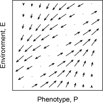
This vector field corresponding to the dual landscape of figure 2 is shown in figure 3.
Vector field of dual landscape model for niche construction (here the model describes immune escape; see sec. 3.1). Vectors combine the actions of adaptation and niche construction. Part of the space is shown, but the phenotype and environment can evolve indefinitely in this system.

Here is a more informal description of how the model works. First, phenotypic change, due to mutation and selection, is seen in the P dimension (center to upper right, in fig. 2). As evolution occurs, the phenotype moves on this axis. But each evolutionary move on this axis may also affect the environment in which subsequent evolution occurs. Change to the environment is represented in the E dimension (center to upper left, in fig. 2). A single episode of change may involve moves in both dimensions, and the new state of the system will be represented by a position along both axes. In figure 2 we draw two landscapes, one above the other. The vertical pole indicates that the system as a whole is subject to two kinds of change. Each new state of the evolving population will be due to the previous phenotype and the previous state of the environment; each new state of the environment will be due to the same two factors. Change “uphill” on the phenotypic axis is change in the direction of increased fitness. This raises the question of what “uphill” means on the environment axis. In a very loose sense, a peak on the environment dimension is analogous to a point of high fitness—it is a point that tends to be reached from neighboring points, a local “attractor.” Phenotypes of high fitness are “attractors” in systems governed by differential reproduction and heredity. Environmental states, whether biotic or abiotic, can be attractors, too, for different reasons. We will illustrate these relationships with some examples from microbial evolution.
3. Applications and Illustrations
In this section we describe three applications of the dual landscape concept. These applications are in microbial evolution, and they exhibit a range of dynamical behaviors.
3.1. Antigenic Evolution and Immune Memory
First, we present an application of the dual landscape concept to the niche construction that occurs as pathogens influence the state of immune memory in their hosts and, as a result, undergo evolution in their antigens through the process of immune escape. In this example, the phenotype P is the antigen state of the pathogen, and the environment E is the immune memory state of the host population. The pathogen and host populations are each assumed to be monomorphic. Let w be the underlying fitness of a pathogen strain that has never been encountered in a host population. Let there be a fitness cost to the pathogen of being recognized by host immune memory; this cost is greatest when the strain is exactly the same as what the population previously encountered and smaller when the strain is antigenically similar but not identical to the previous strain. If σ is the degree of cross-immunity, the fitness function might be

which has a low-fitness trough where P and E are similar. This adaptive landscape models how pathogens escape the host immune response via mutation. The host environment is the state of immune memory in the population, and the niche constructive landscape is highest for states “matching” the pathogen. This function might be

where v is an underlying benefit to the host through the action of the immune system and ρ is a factor describing cross-immunity from the host point of view. This constructive landscape has a ridge where P and E are similar, due to the advantage to the host of acquiring memory to recognize P. The forms of these models are similar to the many-strain models that appear in the pathogen evolution literature (Gog and Grenfell Reference Gog and Grenfell2002).
The two surfaces shown in figure 2 are actually computed from the model here, as is the vector field in figure 3. (For simplicity, here and for subsequent examples we assume that
 .) Here, niche construction leads to an arms race in which the pathogen evolves by escaping the immune memory of the host, and the host immune memory responds by developing immunity against new strains of the pathogen. In this never-ending process the pathogen never reaches its adaptive peak because the environment keeps shifting away under its own action. As described for figure 1B this describes an organism that climbs a gravel-covered hill that gives way with each step. An alternative but still loose metaphor is that the organism here is a surfer riding a wave: gravity pulls the surfer in one direction while the force of the wave pushes the board in another. The action of these separate forces on the same object is analogous to the two evolutionary forces acting on organisms in dual landscapes.
3.2. Ameliorating the Environment by Degrading Toxins
Suppose the environment of a bacterial population contains a toxin or antibiotic. Niche constructing bacteria can degrade the antibiotic, thereby improving their environment. The variable P (where
 ) tracks this ability, while E (
 ) tracks the quality of the environment, so that higher values of E correspond to higher rates of detoxification and lower concentrations of the antibiotic. We assume this ability comes with a fitness cost c. To outcompete non-niche constructors that would benefit from the improved environment without suffering the cost, niche constructors must be able to monopolize the improvement to some extent (Krakauer, Page, and Erwin Reference Krakauer, Page and Erwin2009; Conlin, Chandler, and Kerr Reference Conlin, Chandler and Kerr2014). Let m be the viability cost incurred by nondetoxifiers when the environment is in the most toxic state, and let w be a constant that scales the fitness. The parameter m can also be seen as the ability of detoxifiers to monopolize the improved environment they help to create. The fitness of bacteria is then

The bacteria improve the environment in proportion to the niche constructing ability P, and we assume a diminishing return to the environment so that only small improvements can be made to an already very clean environment. Additionally, let the environment be deteriorated by the influx of toxins at a rate δ per unit E. The constructive landscape function can thus be

where q is the maximum environmental quality that can be achieved when
 .
A vector field corresponding to this model is shown in the right panel of figure 4. Here, the environment is detoxified by the organism, but this improvement is countered by an influx of toxin from external sources when the organism is a weak detoxifier. For trajectories that cross the null isocline, bacteria with a weaker ability to degrade are favored over more efficient degraders that bear a higher fitness cost of this ability. The trajectories reach the maximum value of E and then approach the equilibrium, which is at the intersection of the
 null isocline (dashed curve) and the dE/dt = 0 null isocline (solid curve). This equilibrium, which is an evolutionarily stable strategy for the organism, is revealed by the dual landscape.
Dual landscape and vector field of a model of the evolution of microbes that improve their environment by degrading a toxin or antibiotic. Left two panels, adaptive and constructive landscapes with component vectors. Right, vector field in which the components are combined. Dashed curve, null isocline along which
 ; solid curve, null isocline along which
 . Parameters are
 .

3.3. Drug Resistance and Human Behavior
Boni and Feldman (Reference Boni and Feldman2005) modeled the effect of antibiotic drug resistance evolution on human behavior in seeking drug treatment. They identified a feedback through this niche construction process, which leads to complex dynamics. Their microevolutionary model followed allele frequencies in a population. We present a simplified and mesoevolutionary version of this basic idea to show how we can understand it in terms of the dual landscape.
Here, E is the proportion of people who take antibiotics when they are infected with a pathogen. Let P now represent the degree of resistance of a pathogen to a drug. Assume there is a maximum cost c of resistance that applies to the transmission rate of the pathogen that is
 in the absence of the drug. The recovery rate of the host is γ, and the cure rate due to the drug (i.e., the efficacy of the drug) is ε if the infection involves a drug-sensitive pathogen and in general
 .
In the absence of treatment and drug resistance, the fitness of the pathogen is given by its basic reproduction number
 . With the possibility of drugs in the environment, the expected fitness of a pathogen is

The left term gives the fitness component when the antibiotic is used, and the right term gives the fitness component in the absence of the antibiotic.
The constructive landscape is given by the benefit or utility to human hosts of taking or not taking antibiotic drugs. The benefit of taking antibiotics is proportional to the drug sensitivity of the pathogen,
 . The benefit of not taking drugs is an increasing function of the degree of resistance to the drug, P. The benefit derives from saving money on ineffective drugs and from cultural values that favor restraint in the liberal use of drugs. This restraint stems from understanding that drug use contributes to the rise of resistance. We let this benefit be ηPk, where k models the reluctance of people to refrain from taking antibiotics and η is a proportionality constant that puts this benefit on the same scale as the benefit of taking drugs. If
 , people are unwilling to give up the antibiotic unless there is complete resistance, and if
 , people readily refrain from using the antibiotic if the pathogen becomes partially resistant. Putting these benefits together, we have

The left term is the benefit component when antibiotics are used, and the right term is the benefit component when antibiotics are not used.
A vector field for this model is shown in figure 5. In addition to the vectors, this figure shows the two isoclines along which
 (dashed curve) and
 (vertical line). The feedback induced by niche construction leads to oscillation in the dynamics as the system tips from sensitive pathogens and high levels of drug use to resistant pathogens and low levels of drug use and back again. This seesaw-like behavior is the same as that described in figure 1C.
Dual landscape and vector field of model of niche construction in the evolution of drug resistant pathogens. Left two panels, adaptive and constructive landscapes with component vectors. Right, vector field in which the components are combined. Solid line, null isocline along which
 ; dashed curve, null isocline along which
 . Parameters are
 .

4. Discussion
4.1. A Restoration of Landscapes?
This article seeks to reconcile the concept of the fitness or adaptive landscape with the dynamics of niche construction, which focuses on changes induced by organismic action on environments. In particular, we have sought to make Lewontin’s original mathematical description of niche construction (eq. [1]) not just a heuristic but a concrete framework (eqq. [2] or [3]) for showing how evolutionary feedback can arise. The resulting system can be interpreted according to the dual landscape concept that displays the operation of niche construction at the mesoevolutionary level of multiple successive substitutions (as does the adaptive dynamics approach to evolution). This approach can be applied to a range of niche construction processes that operate at such timescales that can be investigated through a pair of continuous variables describing a phenotype and an environmental variable.
We introduce the dual landscape concept as a partial solution to the problem of dynamic landscapes. An advantage of this concept is that it restores landscapes as static objects, thus making it easier to understand the dynamics of niche construction. While the dual landscape may help us to separate and reintegrate niche construction and adaptation as distinct forces (see fig. 2), it is arguably difficult to see their global action in the phenotype-environment space. The vector field is an equivalent way to present the dynamics, and it may be more useful in that it shows more quantitatively how evolutionary change occurs over the whole space. It also shows how evolutionary feedback occurs due to organism-driven environmental change.
What is a good metaphor for evolution, particularly under the action of niche construction? Even though a vector field may be a more precise representation of a given model, a landscape may have greater intuitive appeal. For example, the visual metaphor of the dual landscape illustrates in a concrete way how the direction of phenotypic evolution can reverse, while climbing up a gradient occurs continuously on the adaptive landscape. The distinction between metaphors and models is not clear-cut (Calcott Reference Calcott2008). Lewontin (Reference Lewontin1963) suggested that metaphors have a didactic role and should be based on assumptions of a model. Because metaphors carry elements that do not reflect reality, he cautions against building models from a metaphor. While metaphors are less precise and sometimes more misleading than mathematical models, they may serve to help us understand those models. In that way, a metaphor such as the adaptive landscape can perhaps be viewed as a model of a model.
4.2. Limitations and Extensions
The dual landscape model has limitations shared with other smooth phenotype-based fitness landscape models. Phenotype occupies a low dimensional continuous space, and movement occurs by small increments between neighboring phenotypic states. In reality multiple phenotypes would be under selection, and movement between states ultimately depends on the underlying genetics. We have had to assume a simple correspondence between genotype and phenotype so that mutation too is a simple process. But the functional relationship between genotype and phenotype is complex. An important complexity is epistasis: the interaction between fitness effects at multiple genetic loci leads to ruggedness in genotype-based landscapes (Kauffman and Levin Reference Kauffman and Levin1987; Nahum et al. Reference Nahum, Godfrey-Smith, Harding, Marcus, Carlson-Stevermer and Kerr2015). Genotype-based landscapes are multidimensional, with states that are not neatly ordered as in phenotype-based landscapes. When recombination is possible, movement on the landscape is not as straightforward as it is under incremental mutation steps. In particular, large steps on the landscape are possible (Cooper and Kerr Reference Cooper and Kerr2016). Phenotype landscapes therefore conceal some potentially important details at the genetic level.
Nevertheless, simple phenotype-based landscapes play an important role in strengthening our understanding of complex evolutionary processes. Furthermore, while the dual landscapes would be impossible to draw for higher dimensional phenotypes, the mathematical model could be extended readily. A future development could be to extend and generalize the dual landscape concept to genetic models.
The dual landscape model can be extended in other ways. Coevolution between species is recognized to be an important instance of niche construction in which each species is a component of the other species’ environment (Odling-Smee et al. Reference Odling-Smee, Laland and Feldman2003). In the examples we presented here, we left out coevolution, which is already well studied. Instead, we considered processes in which the environment is abiotic (the presence of a toxin or antibiotic) or biotic but changes through nongenetic processes (adaptive host immune response or host behavior). The notion of a dual landscape can be applied to coevolution in which the application is clearly a natural one: each species has its own adaptive landscape, which is a function of the environment that includes the other species (see also Kauffman and Johnsen Reference Kauffman and Johnsen1991; Doebeli Reference Doebeli, Svensson and Calsbeek2012). In principle, the idea can be extended to multiple species and entire ecosystems. It is difficult to actually imagine multiple surfaces over many dimensions, but this objection applies equally to the case of a single fitness landscape over a space of multidimensional traits.
Another extension of our model is to consider landscapes as functions of allele frequencies rather than phenotypes. The interpretation would be different since the variables would model microevolutionary change in allele frequencies over shorter timescales instead of mesoevolutionary change in phenotypes over longer timescales. Furthermore, the landscapes indicate directions of change but no longer describe fitness. The two landscapes would, however, be smooth surfaces with corresponding vector fields. To outline this idea, in appendix A we describe a simple model of two interacting species—each forming the environment of the other species—following frequencies of two alleles in each population.
4.3. Unified Landscapes and Fisher’s Fundamental Theorem
In general there is no unified landscape to describe niche construction. That is, in a given system it is usually not possible to find a single landscape to capture the dynamical behavior of the system. This is because there is no single surface that behaves like a potential function in physics, where vector fields are conservative and integrals around closed curves equal zero, which applies, for example, to systems with energy conservation. While the parallels between evolution and statistical physics have been noted (e.g., by Walsh, Lewens, and Ariew [Reference Walsh, Lewens and Ariew2002] and more formally by Sella and Hirsh [Reference Sella and Hirsh2005]), for niche construction and adaptation there is in general no potential function unless

which would not hold except by serendipity or artifice.
This feature then imposes an inherent limitation on landscapes as a heuristic tool. There is no single landscape that behaves like a real topographic landscape or an energy potential. It also highlights that two distinct forces operate in the evolutionary dynamics we consider here: niche construction and adaptation. We reiterate that the utility of the dual landscape as an aid to intuition is that it separates the two evolutionary forces and reintegrates them in the manner shown in figure 2.
The notion of a unified landscape has connections with Fisher’s fundamental theorem of natural selection (FTNS; Fisher Reference Fisher1999). Under the modern interpretation of the FTNS, the total change in fitness is made of two parts: the change in fitness due to natural selection and the remaining change due to the deterioration of the environment (Price Reference Price1972; Ewens Reference Ewens1989, Reference Ewens2010; Frank and Slatkin Reference Frank and Slatkin1992; Okasha Reference Okasha2008; Frank Reference Frank, Svensson and Calsbeek2012), where “environment” is broadly defined to include some genetic effects beyond additive effects at the gene in question (Price Reference Price1972; Okasha Reference Okasha2008, Reference Okasha2010). In appendix B we show that under a specific interpretation of FTNS the mean fitness ϕM(P, E) is satisfied by the differential equations

Here, there is a single unified surface ϕM(P, E) that links environmental deterioration and adaptation.
5. Conclusion
By defining a constructive landscape that describes environmental states that tend to be produced by organic activities, and by defining an adaptive landscape that is also a function of the environment, we are able to employ a static conception of landscapes. This enables tools to be used that would be unavailable in other frameworks. In particular, while a dynamic trampoline-like adaptive landscape is intuitively helpful to some extent, the deformations of such surfaces are not clearly defined. When a person steps on a trampoline, the surface is always depressed. When a species modifies the environment, however, the adaptive landscape will sometimes rise and other times sink, depending on the form of niche construction operating in that case. Our dual landscape model can specify these different sorts of change, and their evolutionary consequences, in a precise manner. The most important step enabled by our discussion is the move from purely heuristic and intuitive ways of thinking about organism-environment coupling to a framework in which the relations between adaptive and constructive change can be represented flexibly and precisely.
Appendix A. Dual Landscape over Allele Frequencies
To outline a dual landscape concept over allele frequencies rather than phenotypes, we give details of a one-locus haploid model of exploiters and victims as a niche construction system. Specifically, imagine two interacting species—a prey species and its predator—each with a single diallelic locus. Genotype B of the predator is dependent on genotype A for food—when A is abundant, then B has a higher fitness than b (which uses another more reliable species for food). Genotype a of the prey is resistant to predation by genotype B but pays a cost for the resistance. Thus, when B is abundant, a has an advantage over A, but when b is abundant A has an advantage over a. If the frequency of prey genotype A at time t is given by p(t) and predator genotype B at time t is given by q(t) and if the simplest form of frequency dependent fitnesses are assumed, this coevolving system can be described by the following difference equations:

which can be approximated with ordinary differential equations by considering changes in the two variables over the period Δt. That is, we calculate

which simplify to yield

The dual landscapes for these functions are found by integrating these two quantities with respect to p and q:

where Cp and Cq are integration constants. Figure A1 shows dynamics of allele frequencies in the two populations on these dual landscapes.
Dual landscape for a coevolving predator-prey community. Dynamics of genotype proportions, governed by differential equations (A1), are shown on the lower p-q plane. The landscape for each species is shown in different colors (prey in light gray and predator in dark gray). Arrows indicate the gradient in the relevant landscape, and both arrows are also projected into the p-q plane. Dynamics involve continual cycling of genotype frequencies.

Appendix B. Niche Construction and Fisher’s Fundamental Theorem
To show how Fisher’s fundamental theorem relates to the dual landscape model, let us consider the change in a population resulting from a change in phenotype P, which we assume has a simple relationship with underlying genetic states. Let ϕM, representing the mean fitness of the population, be a function of both phenotype P and environment E. Interpreting Frank’s expression of FTNS (see Frank and Slatkin Reference Frank and Slatkin1992, eq. [2]) with our notation,

where ΔP and ΔE denote the change in mean phenotype and environment, respectively, in a period of time Δt. The two terms in brackets correspond to the two partial change terms in Frank’s expression; the first of these is equal to the additive genetic variance in fitness. In the continuous limit as
 , we obtain a form similar to that given by Price (Reference Price1972):

(dropping (P, E) for convenience), which is simply the chain rule applied to the total change in mean fitness,
 .
Frank and Slatkin (Reference Frank and Slatkin1992) stress that Fisher intended the total change in fitness to be near zero because the rise in mean fitness due to natural selection is balanced by deterioration of the environment. This reading suggests that Fisher regarded the fundamental theorem as a conservation principle requiring that

which occurs, for example, when

These relationships imply that the system is a Hamiltonian under which ϕM is constant (conserved) over time and trajectories follow contours of ϕM.
Thus, the FTNS considers a single fitness function ϕM unlike the dual landscape model (eq. [2]), which involves two landscapes without a unified fitness surface. Under niche construction, fitness conservation does not necessarily hold, and organisms can alter the environment in such a way as to improve their absolute fitness or damage the environment and lower their fitness. Interestingly, the above version of the FTNS is reminiscent of the antigen escape model (sec. 3.1), which we described with the metaphor of an organism climbing a gravel-covered hill that gives way with each step, balancing the ascent with environmental deterioration. Mathematically, the two components can be artificially balanced by specifying that
 and
 (and
 ), so that

implying that a Hamiltonian function exists that can serve as a unified landscape. Hence, under some conditions, negative niche construction is similar to some readings of the FTNS.
Without a conservation principle a population would increase without bound or go extinct (Frank and Slatkin Reference Frank and Slatkin1992; Fisher Reference Fisher1999). If, however, we relax the conservation condition and consider the FTNS as a description of the joint dynamics of the organism and the environment, the result is the dual landscape, which is a more detailed version of Lewontin’s generic equations for niche construction (eq. [1]).