1 Introduction
The stability of steady columnar rotating flows that have a non-zero azimuthal velocity component
 $u_{{\it\theta}}^{C}(r)$
(where
 $r$
is the radial distance from the centreline) with no axial velocity component, either in pipes or between two coaxial rotating cylinders, is a classical problem in fluid mechanics. Kelvin (Reference Kelvin1880) studied the propagation of axisymmetric and three-dimensional normal-mode waves on a solid-body rotation flow in a pipe based on the inviscid flow formulation. He found that the waves are always bounded with neutral oscillations. Rayleigh (Reference Rayleigh1916), and later on Synge (Reference Synge1933), also used the inviscid flow formulation and the normal-mode waves approach to establish a general necessary and sufficient criterion for the linear stability of columnar rotating flows to axisymmetric perturbations. This criterion requires that the Rayleigh discriminant
 ${\it\Phi}(r)$
be strictly positive, i.e.
 ${\it\Phi}=(2K^{C}/r^{3})\,\text{d}(K^{C})/\text{d}r>0$
, in the entire flow radial domain. This classical inviscid linear stability criterion is directly related to the monotonicity of the circulation function
 $K^{C}(r)$
, where
 $K^{C}(r)=ru_{{\it\theta}}^{C}(r)$
is the circulation function of the base columnar rotating flow.
Of specific interest to the present paper is the circular Couette flow between two coaxial rotating cylinders (Couette Reference Couette1890; Taylor Reference Taylor1923; see also Chandrasekhar Reference Chandrasekhar1961). Under certain radii and angular speeds of the cylinders, specifically when they are co-rotating, this flow becomes unstable and forms the well-known axisymmetric Taylor vortices (see e.g. figure 1 in Andereck, Liu & Swinney (Reference Andereck, Liu and Swinney1986) and figure 3.7 in Drazin & Reid (Reference Drazin and Reid2004), p. 106). We note that (Taylor Reference Taylor1923) studied the case of a flow in a narrow gap between two coaxial rotating cylinders with normal-mode analysis and determined the linear marginal stability line for the viscous rotating flow in terms of its operational parameters.
The linear stability and the loss of stability of the circular Couette flow have been thoroughly studied over the years in many experiments. It revealed a complex transition state diagram in terms of Reynolds numbers of the inner and outer cylinders,
 $R_{i}$
and
 $R_{o}$
, respectively (based on the speed of rotation and the radius of each cylinder). For example, the detailed experiments in Andereck et al. (Reference Andereck, Liu and Swinney1986) found the appearance of various stable axisymmetric wavy states when the cylinders are co-rotating. These various states change from one to another when the Reynolds number of the inner cylinder is increased above a certain limiting value, which also depends on the outer cylinder’s Reynolds number. The loss of stability in these situations is dominated by the mechanism for the appearance of the Taylor vortices; see also Krueger, Gross & Di Prima (Reference Krueger, Gross and Di Prima1966), who found that the base circular Couette flow is unstable to critical axisymmetric perturbations when the ratio of the outer rotational speed to the inner rotational speed is above
 $-0.78$
. On the other hand, when the cylinders are counter-rotating, and the outer cylinder’s Reynolds number is sufficiently large in size,
 $R_{o}<-140$
, a variety of non-axisymmetric unsteady wave states and turbulent states appear as the inner Reynolds number is increased above another limiting value. The loss of stability in these situations is dominated by three-dimensional spiral waves. This result is supported by the linear stability analysis by Krueger et al. (Reference Krueger, Gross and Di Prima1966), who showed that the base circular Couette flow is unstable to non-axisymmetric perturbations when the ratio of rotational speeds is below
 $-0.78$
.
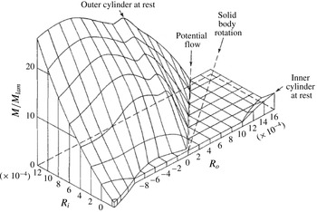
The experiments also revealed that, within a certain range of Reynolds numbers (of the inner and outer cylinders), the measured torque applied to the cylinders is the same as the theoretical torque for a laminar, axisymmetric, stable circular Couette flow (see e.g. figure 1 in Coles (Reference Coles1965) displaying the reproduced experimental results by Wendt (Reference Wendt1933)). These classical experimental results indicated that, within this range of Reynolds numbers, the viscous flow between the two coaxial rotating cylinders evolves to the standard circular Couette flow, where it remains axisymmetric, and is stable not only to infinitesimally small perturbations but also to finite-amplitude perturbations. The stable operational range of the circular Couette flow is limited by Rayleigh’s (Reference Rayleigh1916) inviscid linear stability criterion. The stable region also appears in the detailed diagram of states in figure 1 of Andereck et al. (Reference Andereck, Liu and Swinney1986). This raises a need for a theoretical study regarding the evolution of finite-amplitude perturbations on the circular Couette flow, specifically in the stable operational range. The theoretical explanation of this nonlinear phenomenon may offer further insight into the underlying flow dynamics and may also deepen our understanding of the existing experimental observations.
The nonlinear stability of the viscous circular Couette flow in response to axisymmetric finite-amplitude perturbations was studied in the classical paper by Serrin (Reference Serrin1959) and then revisited by Joseph & Hung (Reference Joseph and Hung1971). Serrin (Reference Serrin1959) applied the Reynolds–Orr equation and derived a formula for the rate of change in time of the perturbation’s kinetic energy integral
 $\tilde{\mathscr{E}}$
. Based on this formula, he showed that, when the viscosity of the fluid
 ${\it\nu}$
is greater than a certain level
 ${\it\nu}_{\tilde{\mathscr{E}}}$
(which depends on the operational conditions), the viscous dissipation alone can overcome the inviscid nonlinear energy production term that results from the interaction between the perturbation and the base flow. Thereby he ensured a monotonic temporal decay of
 $\tilde{\mathscr{E}}$
, and determined a definite range in terms of the operational Reynolds numbers of the cylinders for which any initial axisymmetric finite-amplitude perturbation decays monotonically in time. The global nonlinear stability region by Serrin (Reference Serrin1959) forms a fixed band of operational parameters around the solid-body rotation flow set-up, and is significant only when the operational Reynolds numbers are relatively small. However, in the case of high Reynolds numbers, the band is relatively small and the circular Couette flow must be sufficiently close to the solid-body rotation flow in order for its parameters to be within Serrin’s (Reference Serrin1959) stability band.
Joseph & Hung (Reference Joseph and Hung1971) followed Synge’s linear stability analysis (Synge Reference Synge1938a
,Reference Synge
b
) of the viscous circular Couette flow in response to axisymmetric perturbations. They established a formula for the rate of change in time of a weighted kinetic energy integral of the perturbation
 $\tilde{\mathscr{E}}_{w}$
. Their formula revealed two essential physical mechanisms that govern the rate of change in time of
 $\tilde{\mathscr{E}}_{w}$
, which is composed of the viscous dissipation and a nonlinear (cubic-order) inviscid energy production term that results from the interaction between the velocity perturbations. When the perturbation’s size is small with respect to the viscous damping effect, they found that nonlinear stability is guaranteed by the condition for linear stability, including the inviscid borderline for linear stability. This result is relevant to flows where the operational Reynolds numbers are relatively small, and hence viscous stresses can dissipate large finite-amplitude perturbations. However, the initial size of the perturbation in their result is not global and is always limited by the value of the fluid viscosity. At high operational Reynolds numbers, Joseph & Hung’s (Reference Joseph and Hung1971) restriction on the initial size of
 $\tilde{\mathscr{E}}_{w0}$
becomes severely limited and may not apply to realistic perturbations (unless the flow is sufficiently close to the solid-body rotation flow).
The objectives of this present paper are: (i) to develop an axisymmetric viscous nonlinear stability analysis that extends Joseph & Hung’s (Reference Joseph and Hung1971) approach; (ii) to determine theoretically the largest possible global nonlinear stability region for the circular Couette flow to any initial finite-amplitude axisymmetric perturbation (in terms of its operational parameters); and (iii) to extend Serrin’s (Reference Serrin1959) prediction for the axisymmetric nonlinear stability region of the viscous circular Couette flow. To achieve this goal, we use the Arnol’d energy-Casimir method and thereby define a different weighted kinetic energy integral of the perturbation
 $\tilde{\mathscr{E}}\rfloor _{{\it\xi}}$
, which was originally defined in Wang (Reference Wang2009). We find in the present study that the weighted kinetic energy integral of the perturbation
 $\tilde{\mathscr{E}}_{w}$
used by Joseph & Hung (Reference Joseph and Hung1971) is only a linearized form of the present weighted kinetic energy integral of the perturbation
 $\tilde{\mathscr{E}}\rfloor _{{\it\xi}}$
. In this sense, the present study is closely connected with the result by Joseph & Hung (Reference Joseph and Hung1971), and hence formulates a comprehensive nonlinear extension of their theory.
In the study of flow nonlinear stability, Arnol’d (Reference Arnol’d1965, Reference Arnol’d1969) was the first to formulate an energy-Casimir function to examine the dynamics of finite-amplitude perturbations on two-dimensional inviscid parallel shear flows. He established conditions for the nonlinear stability of such flows; see also Arnol’d & Khesin (Reference Arnol’d and Khesin1998) for a detailed treatment of this problem using Lie algebra and symmetry reduction. These mathematical concepts form the basis of the Arnol’d energy-Casimir method. Abarbanel et al. (Reference Abarbanel, Holm, Marsden and Ratiu1986) extended the Arnol’d energy-Casimir method to study the nonlinear stability of steady two-dimensional columnar flows of a stratified fluid. Conditions for the nonlinear stability of inviscid columnar rotating flows were first established in Vladimirov (Reference Vladimirov1986a ,Reference Vladimirov b ) by using a perturbation norm (which includes a fourth power of the azimuthal velocity perturbation) and the Arnol’d energy-Casimir method. Szeri & Holmes (Reference Szeri and Holmes1988) applied the Arnol’d energy-Casimir method to axisymmetric inviscid columnar rotating flows and developed a general form of the Arnol’d function, where it was used to study the inviscid flow nonlinear stability of columnar rotating flows with a general axial velocity profile.
The linear stability of inviscid columnar rotating flows has been studied by Kloosterziel, Carnevale & Orlandi (Reference Kloosterziel, Carnevale and Orlandi2007). They developed a Lyapunov function and found that Rayleigh’s (Reference Rayleigh1916) classical inviscid linear stability criterion also leads to Lyapunov stability of the flow when infinitesimally small perturbations are considered, which is stronger than spectral stability (derived from the normal-mode analysis). By considering the linearized axisymmetric viscous flow equations, Kloosterziel (Reference Kloosterziel2010) extended the approach to study the linear stability properties of viscous circular flows in rotating environments to axisymmetric perturbations. He derived sufficient conditions for Lyapunov stability with respect to such perturbations. It should be noted that the Lyapunov function used by Kloosterziel (Reference Kloosterziel2010) has the same form as the weighted kinetic energy integral of the perturbation
 $\tilde{\mathscr{E}}_{w}$
used by Joseph & Hung (Reference Joseph and Hung1971), which is the linearized form of the present weighted kinetic energy integral of the perturbation
 $\tilde{\mathscr{E}}\rfloor _{{\it\xi}}$
. However, since Kloosterziel’s (Reference Kloosterziel2010) analysis was essentially based on the linearized flow dynamics, it cannot be extended to study the nonlinear stability of viscous columnar rotating flows.
The nonlinear stability of inviscid columnar rotating flows was also studied in Wang (Reference Wang2009). It is noted that the norm used by Wang (Reference Wang2009) for the perturbation is based on the difference of the reduced Arnol’d function
 ${\rm\Delta}\mathscr{A}_{rd}$
that was originally formulated in Szeri & Holmes (Reference Szeri and Holmes1988). In the present paper, we extend the analysis of Wang (Reference Wang2009) to study the nonlinear stability of the viscous circular Couette flow to axisymmetric finite-amplitude perturbations. The basic idea is (i) to use the weighted kinetic energy integral of the perturbation
 $\tilde{\mathscr{E}}\rfloor _{{\it\xi}}$
(derived from the difference of the reduced Arnol’d function
 ${\rm\Delta}\mathscr{A}_{rd}$
by Wang (Reference Wang2009)) as a Lyapunov function for the case of a viscous circular Couette flow, and (ii) to identify a definite nonlinear stability region for the circular Couette flow in terms of its operational parameters where this Lyapunov function decays monotonically in time. The current weighted kinetic energy integral of the perturbation
 $\tilde{\mathscr{E}}\rfloor _{{\it\xi}}$
is invariant in the inviscid flow nonlinear dynamics (see Wang Reference Wang2009). We also find that the weighted kinetic energy integral of the perturbation
 $\tilde{\mathscr{E}}_{w}$
used in Joseph & Hung (Reference Joseph and Hung1971) and Kloosterziel (Reference Kloosterziel2010) is a linearized form of the difference of the reduced Arnol’d function
 ${\rm\Delta}\mathscr{A}_{rd}$
, and is, therefore, invariant only in the linearized inviscid flow dynamics. The advantage of the current analysis stems from a newly derived formula that relates the rate of change in time of the present Lyapunov function to only the viscous perturbation terms. There is no inviscid nonlinear energy production term in this formula, such as the cubic-order energy production term found in Joseph & Hung’s (Reference Joseph and Hung1971) formulation.
It should be noted that the viscous terms may affect the nonlinear dynamics of the flow in a complicated way. Unlike the approaches by Joseph & Hung (Reference Joseph and Hung1971) and Kloosterziel (Reference Kloosterziel2010), the viscous effect found in the present study does not necessarily induce only damping on the present weighted kinetic energy integral of the perturbation,
 $\tilde{\mathscr{E}}\rfloor _{{\it\xi}}$
. For estimating the viscous effects, we first derive two basic flow identities for the temporal rate of change of the total kinetic energy integral,
 $\mathscr{E}$
, and of the circulation-dependent integral (Casimir’s integral),
 $\mathscr{C}_{S}$
. We then combine these identities to form the formula for the temporal rate of change of the weighted kinetic energy integral of the perturbation, which contains only viscous terms. By carefully examining these viscous terms, we establish a definite stability region for the circular Couette flow (independent of the fluid viscosity), where it is nonlinearly stable in response to any axisymmetric finite-amplitude perturbation (provided that the initial total circulation function
 $K(x,y,t=0)$
remains above a certain minimum level that is determined by the operational parameters of the circular Couette base flow).
The outline of this paper is as follows. In § 2, we formulate the mathematical flow problem and identify the base steady classical circular Couette flow solution. In § 3.1, we summarize the results by Wang (Reference Wang2009) for the nonlinear stability condition of an inviscid columnar rotating flow. In § 3.2, we derive the two flow identities for the temporal rate of change of
 $\mathscr{E}$
and of
 $\mathscr{C}_{S}$
. In § 3.3, we combine the results from § 3.2 to form the temporal rate of change of
 $\tilde{\mathscr{E}}\rfloor _{{\it\xi}}$
, then apply it to the case of the viscous circular Couette flow, and derive sufficient conditions for the nonlinear stability of this flow in response to axisymmetric perturbations. In § 3.4, we study these conditions for the linearized flow problem with infinitesimally small perturbations. This establishes a connection between the present study and that by Kloosterziel (Reference Kloosterziel2010). In § 3.5, we derive the nonlinear stability criterion for the circular Couette flow (against axisymmetric finite-amplitude perturbations), and also the corresponding stability region in terms of its operational parameters. In § 4, we discuss the relationship between the present results and the data from experimental studies by Wendt (Reference Wendt1933) (§ 4.1), along with the classical theoretical nonlinear stability results by Serrin (Reference Serrin1959) (§ 4.2.1) and Joseph & Hung (Reference Joseph and Hung1971) (§ 4.2.2). We demonstrate that the present results extend these classical nonlinear stability predictions. In § 5, we derive analytical estimates for the upper bound on the decay rate of finite-amplitude perturbations for two base flow set-ups and describe the results of numerical simulations for various perturbations tested in these set-ups. The conclusions of this paper are summarized in § 6. The appendices provide the derivation details of the identities used in § 3.2, and also a maximum principle used in § 3.5.
2 Problem formulation
We consider an incompressible and axisymmetric rotating flow of a viscous Newtonian fluid in a finite-length cylindrical domain of length
 $L$
between two straight, circular coaxial cylinders of radii
 $R_{1}$
and
 $R_{2}$
(
 $R_{2}>R_{1}$
). In the case when the flow is in a straight circular pipe, then
 $R_{1}=0$
is assumed. We use the cylindrical coordinates
 $(r,{\it\theta},x)$
, where the flow domain is given by
 $V=\{(r,{\it\theta},x):R_{1}<r<R_{2},0\leqslant {\it\theta}<2{\rm\pi},0<x<L\}$
. The velocity vector is given by
 $\boldsymbol{u}=(u_{r},u_{{\it\theta}},u_{x})$
with the radial, azimuthal and axial components, respectively. The pressure field is denoted as
 $p$
. The density of the fluid is denoted as
 ${\it\rho}$
, the dynamic viscosity and the kinematic viscosity are given by
 ${\it\mu}$
and
 ${\it\nu}={\it\mu}/{\it\rho}$
respectively, and they are all assumed to be constant.
Let
 $y=r^{2}/2$
, with
 $y_{1}=R_{1}^{2}/2$
and
 $y_{2}=R_{2}^{2}/2$
, and the flow domain is given by
 $D=\{(x,y):0<x<L,y_{1}<y<y_{2}\}$
. The incompressible axisymmetric Navier–Stokes equations in terms of
 $(x,y,t)$
are written as
 $$\begin{eqnarray}\displaystyle & \displaystyle \sqrt{2y}\frac{\partial u_{r}}{\partial y}+\frac{u_{r}}{\sqrt{2y}}+\frac{\partial u_{x}}{\partial x}=0, & \displaystyle\end{eqnarray}$$
 $$\begin{eqnarray}\displaystyle & \displaystyle \frac{\partial u_{r}}{\partial t}+u_{r}\sqrt{2y}\frac{\partial u_{r}}{\partial y}+u_{x}\frac{\partial u_{r}}{\partial x}-\frac{u_{{\it\theta}}^{2}}{\sqrt{2y}}=-\frac{\sqrt{2y}}{{\it\rho}}\frac{\partial p}{\partial y}+{\it\nu}\left({\rm\Delta}u_{r}-\frac{u_{r}}{2y}\right), & \displaystyle\end{eqnarray}$$
 $$\begin{eqnarray}\displaystyle & \displaystyle \frac{\partial u_{{\it\theta}}}{\partial t}+u_{r}\sqrt{2y}\frac{\partial u_{{\it\theta}}}{\partial y}+\frac{u_{r}u_{{\it\theta}}}{\sqrt{2y}}+u_{x}\frac{\partial u_{{\it\theta}}}{\partial x}={\it\nu}\left({\rm\Delta}u_{{\it\theta}}-\frac{u_{{\it\theta}}}{2y}\right), & \displaystyle\end{eqnarray}$$
 $$\begin{eqnarray}\displaystyle & \displaystyle \frac{\partial u_{x}}{\partial t}+u_{r}\sqrt{2y}\frac{\partial u_{x}}{\partial y}+u_{x}\frac{\partial u_{x}}{\partial x}=-\frac{1}{{\it\rho}}\frac{\partial p}{\partial x}+{\it\nu}{\rm\Delta}u_{x}, & \displaystyle\end{eqnarray}$$
 ${\rm\Delta}:=\partial _{y}(2y\partial _{y})+\partial _{xx}^{2}$
is the axisymmetric Laplacian operator in the cylindrical coordinates.
By virtue of the axisymmetry of the flow, a streamfunction
 ${\it\psi}(x,y,t)$
can be defined such that
 $$\begin{eqnarray}\displaystyle u_{r}(x,y,t)=-\frac{1}{\sqrt{2y}}\frac{\partial {\it\psi}}{\partial x},\quad u_{x}(x,y,t)=\frac{\partial {\it\psi}}{\partial y}. & & \displaystyle\end{eqnarray}$$
Using
 ${\it\psi}(x,y,t)$
, the continuity equation (2.1a
) is satisfied automatically. The reduced azimuthal vorticity
 ${\it\chi}$
is given by
 $$\begin{eqnarray}\displaystyle {\it\chi}(x,y,t)=-\!\left(\frac{1}{2y}\frac{\partial ^{2}{\it\psi}}{\partial x^{2}}+\frac{\partial ^{2}{\it\psi}}{\partial y^{2}}\right):=\mathscr{L}{\it\psi}, & & \displaystyle\end{eqnarray}$$
where the azimuthal vorticity is
 ${\it\eta}(x,y,t)=\sqrt{2y}{\it\chi}(x,y,t)$
. The circulation function is
 $K(x,y,t)=\sqrt{2y}\,u_{{\it\theta}}(x,y,t)$
. The equations that relate the evolution of
 ${\it\psi}(x,y,t)$
,
 ${\it\chi}(x,y,t)$
and
 $K(x,y,t)$
can be written from (2.1b
) to (2.1d
) as the Squire–Long system of equations
 $$\begin{eqnarray}\displaystyle & \displaystyle \frac{\partial K}{\partial t}+\{{\it\psi},K\}=-2{\it\nu}y\mathscr{L}K, & \displaystyle\end{eqnarray}$$
 $$\begin{eqnarray}\displaystyle & \displaystyle \frac{\partial {\it\chi}}{\partial t}+\{{\it\psi},{\it\chi}\}=\frac{1}{4y^{2}}\frac{\partial }{\partial x}(K^{2})-2{\it\nu}y\mathscr{L}{\it\chi}+4{\it\nu}\frac{\partial {\it\chi}}{\partial y}, & \displaystyle\end{eqnarray}$$
 $\{f,g\}$
is the canonical Poisson bracket defined by
 $$\begin{eqnarray}\displaystyle \{f,g\}:=\frac{\partial f}{\partial y}\frac{\partial g}{\partial x}-\frac{\partial f}{\partial x}\frac{\partial g}{\partial y}. & & \displaystyle\end{eqnarray}$$
Equation (2.4a
) describes the evolution of the circulation
 $K$
in terms of the interaction between convection and viscous diffusion. Equation (2.4b
) describes the evolution of
 ${\it\chi}$
in terms of the interaction between convection, vorticity stretching (due to the axial gradient of the circulation) and viscous diffusion.
The governing flow equations (2.1a–d
) (or (2.4a
) and (2.4b
)) are studied here under certain boundary conditions. The cylinders’ walls at
 $r=R_{1}$
and
 $r=R_{2}$
are rotating at constant angular speeds of
 ${\it\omega}_{1}$
and
 ${\it\omega}_{2}$
, respectively. No-penetration and no-slip boundary conditions are prescribed along the inner and outer walls, i.e.
 ${\it\psi}(x,y_{1},t)={\it\psi}(x,y_{2},t)=0$
,
 $\partial {\it\psi}(x,y_{1},t)/\partial y=\partial {\it\psi}(x,y_{2},t)/\partial y=0$
,
 $K(x,y_{1},t)=K_{1}={\it\omega}_{1}R_{1}^{2}$
and
 $K(x,y_{2},t)=K_{2}={\it\omega}_{2}R_{2}^{2}$
for all time
 $t$
and
 $0\leqslant x<L$
. Axial periodic boundary conditions are imposed at the cylinder ends at
 $x=0$
and
 $x=L$
, i.e.
 ${\it\psi}(0,y,t)={\it\psi}(L,y,t)$
,
 $\partial {\it\psi}(0,y,t)/\partial x=\partial {\it\psi}(L,y,t)/\partial x$
,
 $K(0,y,t)=K(L,y,t)$
and
 ${\it\chi}(0,y,t)={\it\chi}(L,y,t)$
for all time
 $t$
and
 $y_{1}\leqslant y\leqslant y_{2}$
.
A steady-state solution of (2.1a–d
) (thus also of (2.4a
) and (2.4b
)) with the assumed boundary conditions is the well-known circular Couette flow of a viscous Newtonian fluid between two coaxial rotating cylinders. Using the superscript
 $C$
to indicate a columnar base flow state (which means that the base flow depends explicitly only upon the variable
 $y$
), the velocity profile of this particular columnar base flow is given by
 $$\begin{eqnarray}\displaystyle u_{r}^{C}=0,\quad u_{x}^{C}=0,\quad u_{{\it\theta}}^{C}=Ar+\frac{B}{r}=A\sqrt{2y}+\frac{B}{\sqrt{2y}} & & \displaystyle\end{eqnarray}$$
for
 $0\leqslant x<L$
and
 $y_{1}\leqslant y\leqslant y_{2}$
, where the constants
 $A$
and
 $B$
are
 $$\begin{eqnarray}\displaystyle A=\frac{{\it\omega}_{2}R_{2}^{2}-{\it\omega}_{1}R_{1}^{2}}{R_{2}^{2}-R_{1}^{2}},\quad B=-\frac{({\it\omega}_{2}-{\it\omega}_{1})R_{1}^{2}R_{2}^{2}}{R_{2}^{2}-R_{1}^{2}}. & & \displaystyle\end{eqnarray}$$
For this
 $x$
-independent flow, we also have
 ${\it\psi}^{C}(y)=0$
and
 ${\it\chi}^{C}(y)=0$
in the entire domain
 $D$
and all time
 $t$
. The circulation function for this base flow is
 $K^{C}(y)=2Ay+B$
for
 $0\leqslant x<L$
,
 $y_{1}\leqslant y\leqslant y_{2}$
and all time
 $t$
. According to Rayleigh’s (Reference Rayleigh1916) classical inviscid linear stability criterion, the flow is linearly stable to axisymmetric inviscid perturbations if and only if the discriminant
 ${\it\Phi}=(2K^{C}/r^{3})\,\text{d}(K^{C})/\text{d}r$
is strictly positive throughout the domain
 $R_{1}<r<R_{2}$
. Axisymmetric inviscid linear stability is guaranteed if and only if
 $K^{C}(R_{2})>K^{C}(R_{1})\geqslant 0$
, i.e. the cylinders are required to rotate in the same direction and the circulation function for the base flow at the outer wall must be greater than that at the inner wall.
3 Nonlinear stability of the circular Couette flow
To study the nonlinear stability of the circular Couette flow, we first assume that the perturbed/total velocity vector
 $\boldsymbol{u}(x,y,t)$
is given by a linear combination of the base columnar flow velocity vector
 $$\begin{eqnarray}\displaystyle \boldsymbol{u}^{C}(y)=(0,u_{{\it\theta}}^{C}(y),0) & & \displaystyle\end{eqnarray}$$
and a finite-amplitude velocity perturbation vector
 $\tilde{\boldsymbol{u}}(x,y,t)$
, i.e.
 $$\begin{eqnarray}\displaystyle \boldsymbol{u}(x,y,t)=\boldsymbol{u}^{C}(y)+\tilde{\boldsymbol{u}}(x,y,t). & & \displaystyle\end{eqnarray}$$
The radial, axial and azimuthal components of
 $\tilde{\boldsymbol{u}}(x,y,t)$
are
 $\tilde{u} _{r}$
,
 $\tilde{u} _{x}$
and
 $\tilde{u} _{{\it\theta}}$
, respectively. We seek to determine the growth or decay of such velocity perturbation around
 $\boldsymbol{u}^{C}(y)$
.
3.1 Nonlinear stability of an inviscid columnar rotating flow
We first summarize the results by Wang (Reference Wang2009), for the axisymmetric inviscid nonlinear stability of a general columnar rotating flow between two coaxial cylinders with axial periodic boundary conditions. A general base columnar rotating flow given by (3.1) was considered. Let
 $\mathscr{E}$
be the total kinetic energy integral of the flow in the domain
 $V$
, which is given by
 $$\begin{eqnarray}\displaystyle \mathscr{E}=\frac{1}{2}{\it\rho}\int _{V}(u_{r}^{2}+u_{x}^{2}+u_{{\it\theta}}^{2})\,\text{d}V, & & \displaystyle\end{eqnarray}$$
where
 $\text{d}V=r\,\text{d}r\,\text{d}x\,\text{d}{\it\theta}=\text{d}y\,\text{d}x\,\text{d}{\it\theta}$
. It was shown that, under the given boundary conditions and the application of integration by parts,
 $\mathscr{E}$
can also be written as
 $$\begin{eqnarray}\displaystyle \mathscr{E}=\mathscr{E}({\it\chi},K)=\frac{1}{2}{\it\rho}\int _{V}\left({\it\psi}{\it\chi}+\frac{K^{2}}{2y}\right)\text{d}V. & & \displaystyle\end{eqnarray}$$
Note that the boundary term vanishes in the integration because of the preservation of the volume flow rate. In addition, let
 $\mathscr{C}_{S}$
be the circulation-dependent integral (Casimir’s integral) given by
 $$\begin{eqnarray}\displaystyle \mathscr{C}_{S}=\mathscr{C}_{S}(K)={\it\rho}\int _{V}j(K)\,\text{d}V, & & \displaystyle\end{eqnarray}$$
where
 $j(K)$
is any sufficiently smooth function of
 $K$
. In the inviscid flow case,
 $\mathscr{E}({\it\chi},K)$
and
 $\mathscr{C}_{S}(K)$
are both conserved quantities in time during the perturbation’s evolution, i.e.
 $\text{d}\mathscr{E}/\text{d}t=0$
and
 $\text{d}\mathscr{C}_{S}/\text{d}t=0$
for all time
 $t$
.
Let the reduced Arnol’d function
 $\mathscr{A}_{rd}$
introduced in Wang (Reference Wang2009) be defined by
 $$\begin{eqnarray}\displaystyle \mathscr{A}_{rd}({\it\chi},K) & = & \displaystyle \mathscr{E}({\it\chi},K)+\mathscr{C}_{S}(K)\nonumber\\ \displaystyle & = & \displaystyle \frac{1}{2}{\it\rho}\int _{V}\left({\it\psi}{\it\chi}+\frac{K^{2}}{2y}\right)\text{d}V+{\it\rho}\int _{V}j(K)\,\text{d}V.\end{eqnarray}$$
The reduced Arnol’d function
 $\mathscr{A}_{rd}({\it\chi},K)$
is also conserved in time during the perturbation’s inviscid evolution, i.e.
 $\text{d}\mathscr{A}_{rd}/\text{d}t=0$
for all time
 $t$
.
In the formulation of
 $\mathscr{C}_{S}(K)$
, Wang (Reference Wang2009) chose the function
 $j(K)$
such that the first derivative of
 $j(K)$
with respect to
 $K$
(when evaluated at
 $K^{C}$
) satisfies the condition
 $$\begin{eqnarray}\displaystyle \left.\frac{\text{d}}{\text{d}K}\right|_{K=K^{C}}j(K)=-\frac{K^{C}}{2Y(K^{C})}, & & \displaystyle\end{eqnarray}$$
where
 $K=K^{C}(y)$
is the circulation function of a base columnar rotating flow state. For a base flow with a monotonically increasing circulation function
 $K^{C}(y)$
, the function
 $Y(K^{C})$
is the inverse function of
 $K^{C}(y)$
, such that
 $Y(K^{C}(y))=y$
. Note that, for any given base flow, (3.7) is used to formulate the function
 $j(K)$
, and hence the formulation of
 $\mathscr{C}_{S}(K)$
.
The difference of the reduced Arnol’d function
 ${\rm\Delta}\mathscr{A}_{rd}({\it\chi},K):=\mathscr{A}_{rd}({\it\chi},K)-\mathscr{A}_{rd}({\it\chi}^{C},K^{C})$
is also conserved during the perturbation’s inviscid evolution, i.e.
 $\text{d}{\rm\Delta}\mathscr{A}_{rd}/\text{d}t=0$
for all time
 $t$
. Through the special choice of
 $j(K)$
as defined in (3.7), it was found that the first variation of the reduced Arnol’d function vanishes for any base columnar rotating flow. The difference
 ${\rm\Delta}\mathscr{A}_{rd}({\it\chi},K)$
is then determined by the application of the mean value theorem in the second-order Taylor’s expansion (see details in Wang Reference Wang2009), which is given by
 $$\begin{eqnarray}\displaystyle {\rm\Delta}\mathscr{A}_{rd}({\it\chi},K)=\tilde{\mathscr{E}}\rfloor _{{\it\xi}}=\frac{1}{2}{\it\rho}\int _{V}\left(\tilde{u} _{r}^{2}+\tilde{u} _{x}^{2}+\left[1-2y\left.\frac{\text{d}}{\text{d}K}\right|_{K=K\rfloor _{{\it\xi}}}\left(\frac{K}{2Y(K)}\right)\right]\tilde{u} _{{\it\theta}}^{2}\right)\text{d}V,\quad & & \displaystyle\end{eqnarray}$$
where
 $K\rfloor _{{\it\xi}}$
is an intermediate instantaneous function between the circulation function
 $K^{C}(y)$
of the base columnar rotating flow
 $\boldsymbol{u}^{C}(y)$
and the circulation function
 $K(x,y,t)$
of the instantaneous perturbed/total flow
 $\boldsymbol{u}(x,y,t)$
, that is,
 $K\rfloor _{{\it\xi}}=K^{C}(y)+{\it\xi}(t)[K(x,y,t)-K^{C}(y)]$
, for some
 $0<{\it\xi}(t)<1$
. The relationship (3.8) is significant because it involves only the velocity components of the perturbation. It implies that the weighted kinetic energy integral of the perturbation
 $\tilde{\mathscr{E}}\rfloor _{{\it\xi}}$
(on the right-hand side of (3.8)) is also conserved at all times during the flow evolution. This result leads to the following axisymmetric inviscid nonlinear stability criterion (proven in Wang Reference Wang2009):
Criterion 3.1. If a steady base columnar rotating flow satisfies Rayleigh’s (Reference Rayleigh1916) inviscid linear stability criterion in a strict sense, i.e.
 $\text{d}(K^{C}(y)^{2})/\text{d}y>0$
for all
 $y_{1}<y<y_{2}$
, then any finite-amplitude axisymmetric perturbation on the flow must obey the following energy estimate for all times
 $t\geqslant 0$
:
 $$\begin{eqnarray}\displaystyle \frac{1}{2}{\it\rho}\int _{V}(\tilde{u} _{r}^{2}+\tilde{u} _{x}^{2}+{\it\lambda}^{-}\tilde{u} _{{\it\theta}}^{2})\,\text{d}V\leqslant \frac{1}{2}{\it\rho}\int _{V}(\tilde{u} _{r0}^{2}+\tilde{u} _{x0}^{2}+{\it\lambda}^{+}\tilde{u} _{{\it\theta}0}^{2})\,\text{d}V, & & \displaystyle\end{eqnarray}$$
where
 $$\begin{eqnarray}\displaystyle \left.\begin{array}{@{}c@{}}\displaystyle {\it\lambda}^{-}=\min _{\substack{ y_{1}\leqslant y\leqslant y_{2} \\ K_{min}^{C}\leqslant K\rfloor _{{\it\xi}}\leqslant K_{max}^{C}}}\left[1-2y\left.\frac{\text{d}}{\text{d}K}\right|_{K=K\rfloor _{{\it\xi}}}\left(\frac{K}{2Y(K)}\right)\right],\\ \displaystyle {\it\lambda}^{+}=\max _{\substack{ y_{1}\leqslant y\leqslant y_{2} \\ K_{min}^{C}\leqslant K\rfloor _{{\it\xi}}\leqslant K_{max}^{C}}}\left[1-2y\left.\frac{\text{d}}{\text{d}K}\right|_{K=K\rfloor _{{\it\xi}}}\left(\frac{K}{2Y(K)}\right)\right],\end{array}\right\} & & \displaystyle\end{eqnarray}$$
and
 $\tilde{\boldsymbol{u}}_{0}=(\tilde{u} _{r0},\tilde{u} _{x0},\tilde{u} _{{\it\theta}0})$
is the initial velocity perturbation vector field. If, in addition,
 ${\it\lambda}^{-}>0$
, then the perturbation
 $\tilde{\boldsymbol{u}}=(\tilde{u} _{r},\tilde{u} _{x},\tilde{u} _{{\it\theta}})$
(in terms of the norm as defined by the left-hand side of (3.9)) is bounded from above by the initial perturbation
 $\tilde{\boldsymbol{u}}_{0}=(\tilde{u} _{r0},\tilde{u} _{x0},\tilde{u} _{{\it\theta}0})$
(in terms of the norm as defined by the right-hand side of (3.9)) for all times
 $t\geqslant 0$
, which means that the base columnar rotating flow
 $\boldsymbol{u}^{C}(y)$
is nonlinearly stable.
Remark.
In the case discussed here, nonlinear stability is proven with respect to any axisymmetric finite-amplitude perturbation whose initial total circulation function
 $K(x,y,t=0)=K^{C}(y)+\tilde{K}(x,y,t=0)$
is between the minimum and maximum values of the circulation function
 $K^{C}(y)$
for the base columnar rotating flow
 $\boldsymbol{u}^{C}(y)$
.
The inequality (3.9) shows the possible gain of the perturbation’s kinetic energy through the exchange of weighted kinetic energy between the perturbation’s velocity components. In the case of a solid-body rotation flow between the two coaxial cylinders with axial periodic boundary conditions, where
 ${\it\omega}_{1}={\it\omega}_{2}$
and then
 $B=0$
, we have
 $K^{C}=2Ay$
and then
 ${\it\lambda}^{-}={\it\lambda}^{+}=1$
. Then from (3.9), the perturbation’s kinetic energy at a later time
 $t$
equals the initial perturbation’s kinetic energy for all time
 $t$
. This means that, in the case of the solid-body rotation flow between two coaxial rotating cylinders with axial periodic boundary conditions, there is no change in the perturbation’s kinetic energy and no possible growth of any perturbation, as was originally found by the linear stability study of Kelvin (Reference Kelvin1880). However, in all other flows that are stable according to Rayleigh’s (Reference Rayleigh1916) inviscid linear stability criterion, including the circular Couette flow and the Lamb–Oseen vortex, there exists a range of flow parameters where
 $0<{\it\lambda}^{-}<{\it\lambda}^{+}$
. For such flows, the perturbation’s kinetic energy may grow because the perturbation’s azimuthal velocity may convert into radial and axial velocity perturbations. However, this growth is bounded according to (3.9). The inequality (3.9) provides both an estimate and an upper bound for the nonlinear growth of perturbations. From this perspective, (3.9) is also a generalized, axisymmetric, inviscid nonlinear stability criterion for columnar rotating flows.
3.2 Supporting identities for a viscous axisymmetric columnar rotating flow
In this section, we extend the inviscid flow nonlinear stability result by Wang (Reference Wang2009) to a perturbed columnar viscous rotating flow with an axisymmetric finite-amplitude perturbation between two coaxial rotating cylinders, together with axial periodic boundary conditions. We consider the reduced Arnol’d function defined by (3.6) and use the difference given by
 ${\rm\Delta}\mathscr{A}_{rd}({\it\chi},K):=\mathscr{A}_{rd}({\it\chi},K)-\mathscr{A}_{rd}({\it\chi}^{C},K^{C})$
as a Lyapunov function. We look to determine the operational conditions for which
 $\text{d}{\rm\Delta}\mathscr{A}_{rd}/\text{d}t\leqslant 0$
for all times
 $t\geqslant 0$
, and from this to extend the inviscid flow kinetic energy estimates of the perturbation given by the inequality (3.9) to the viscous flow case.
We develop two supporting identities for an axisymmetric viscous columnar rotating flow. In both identities, we consider a base steady, axisymmetric, incompressible, viscous columnar rotating flow in the domain
 $V$
, where
 $u_{r}^{C}=u_{x}^{C}=0$
and
 $u_{{\it\theta}}=u_{{\it\theta}}^{C}(y)$
. The base flow is perturbed according to (3.2).
Identity 3.1. The temporal rate of change of the total kinetic energy integral
 $\mathscr{E}$
(defined by (3.3)) is given by
 $$\begin{eqnarray}\displaystyle \frac{\text{d}\mathscr{E}}{\text{d}t}={\it\mu}(I_{1}+I_{2}), & & \displaystyle\end{eqnarray}$$
where
 $I_{1}$
is the boundary integral containing the first-order perturbation term,
 $$\begin{eqnarray}\displaystyle I_{1}=4{\rm\pi}\int _{0}^{L}\left[yu_{{\it\theta}}^{C}\frac{\partial \tilde{u} _{{\it\theta}}}{\partial y}\right]_{y=y_{1}}^{y=y_{2}}\,\text{d}x, & & \displaystyle\end{eqnarray}$$
and
 $I_{2}$
is the volume integral containing the sum of second-order perturbation terms,
 $$\begin{eqnarray}\displaystyle I_{2}=-\int _{V}\left(\frac{\tilde{u} _{r}^{2}}{2y}+\frac{\tilde{u} _{{\it\theta}}^{2}}{2y}+|\boldsymbol{{\rm\nabla}}\tilde{u} _{r}|^{2}+|\boldsymbol{{\rm\nabla}}\tilde{u} _{x}|^{2}+|\boldsymbol{{\rm\nabla}}\tilde{u} _{{\it\theta}}|^{2}\right)\text{d}V. & & \displaystyle\end{eqnarray}$$
Here, the gradient operator
 $\boldsymbol{{\rm\nabla}}$
written in axisymmetric cylindrical coordinates is given by
 $$\begin{eqnarray}\displaystyle \boldsymbol{{\rm\nabla}}:=\frac{\partial }{\partial x}\boldsymbol{e}_{x}+\sqrt{2y}\frac{\partial }{\partial y}\boldsymbol{e}_{r}, & & \displaystyle\end{eqnarray}$$
with
 $|\boldsymbol{{\rm\nabla}}\tilde{u} _{r}|^{2}:=(\boldsymbol{{\rm\nabla}}\tilde{u} _{r})\boldsymbol{\cdot }(\boldsymbol{{\rm\nabla}}\tilde{u} _{r})=(\partial _{x}\tilde{u} _{r})^{2}+2y(\partial _{y}\tilde{u} _{r})^{2}$
, and similar formulas apply for
 $\tilde{u} _{x}$
and
 $\tilde{u} _{{\it\theta}}$
.
Remark.
The boundary integral
 $I_{1}$
represents the work done by viscous forces along the wall onto the flow due to the presence of the no-slip boundary conditions as a result of viscosity, while the volume integral
 $I_{2}$
reflects the viscous damping effect in the bulk. The derivation of Identity 3.1 is straightforward, and is presented in appendix A for completeness.
Identity 3.2. For any choice of the sufficiently smooth function
 $j(K)$
, the temporal rate of change of the circulation-dependent integral (Casimir’s integral)
 $\mathscr{C}_{S}$
(defined by (3.5)) is given by
 $$\begin{eqnarray}\displaystyle \frac{\text{d}\mathscr{C}_{S}}{\text{d}t}={\it\mu}(S_{1}+S_{2}), & & \displaystyle\end{eqnarray}$$
where
 $S_{1}$
is the sum of integrals containing the first-order terms of the circulation perturbation
 $\tilde{K}=K-K^{C}(y)$
,
 $$\begin{eqnarray}\displaystyle S_{1} & = & \displaystyle 4{\rm\pi}\int _{0}^{L}\left[yj^{\prime }(K^{C})\frac{\partial \tilde{K}}{\partial y}\right]_{y=y_{1}}^{y=y_{2}}\,\text{d}x\nonumber\\ \displaystyle & & \displaystyle -\,2\int _{V}\left[yj^{\prime \prime \prime }(K^{C})\left(\frac{\text{d}K^{C}}{\text{d}y}\right)^{2}\tilde{K}+2yj^{\prime \prime }(K^{C})\frac{\text{d}K^{C}}{\text{d}y}\frac{\partial \tilde{K}}{\partial y}\right]\text{d}V,\end{eqnarray}$$
and
 $S_{2}$
is the sum of integrals containing the higher-order perturbation terms of
 $\tilde{K}$
,
 $$\begin{eqnarray}\displaystyle & & \displaystyle \!\!\!\!S_{2}=-\int _{V}j^{\prime \prime }(K)\left(\frac{\partial \tilde{K}}{\partial x}\right)^{2}\,\text{d}V\nonumber\\ \displaystyle & & \displaystyle \quad -\int _{V}y\left[j^{\prime \prime \prime \prime }(K\rfloor _{{\it\zeta}})\!\left(\left.\frac{\partial K}{\partial y}\right\rfloor _{{\it\zeta}}\right)^{2}\!\tilde{K}^{2}+4j^{\prime \prime \prime }(K\rfloor _{{\it\zeta}})\!\left.\frac{\partial K}{\partial y}\right\rfloor _{{\it\zeta}}\tilde{K}\frac{\partial \tilde{K}}{\partial y}+2j^{\prime \prime }(K\rfloor _{{\it\zeta}})\!\left(\frac{\partial \tilde{K}}{\partial y}\right)^{2}\right]\text{d}V.\nonumber\\ \displaystyle & & \displaystyle\end{eqnarray}$$
Here, the expressions for the intermediate instantaneous functions
 $K\rfloor _{{\it\zeta}}$
and
 $\partial K/\partial y\rfloor _{{\it\zeta}}$
are given by
 $$\begin{eqnarray}\displaystyle \left.\begin{array}{@{}c@{}}\displaystyle K\rfloor _{{\it\zeta}}=K^{C}(y)+{\it\zeta}(t)[K(x,y,t)-K^{C}(y)],\\ \displaystyle \left.\frac{\partial K}{\partial y}\right\rfloor _{{\it\zeta}}=\frac{\text{d}K^{C}(y)}{\text{d}y}+{\it\zeta}(t)\left[\frac{\partial K(x,y,t)}{\partial y}-\frac{\text{d}K^{C}(y)}{\text{d}y}\right],\quad \text{with }0<{\it\zeta}(t)<1.\end{array}\right\} & & \displaystyle\end{eqnarray}$$
Remark.
For a general choice of the sufficiently smooth function
 $j(K)$
, the derivation of Identity 3.2 requires the use of the second-order Taylor’s expansion with a remainder. This derivation uses essential calculus techniques and is shown in appendix B. This identity is new and is applicable for any choice of the sufficiently smooth function
 $j(K)$
. For example, for the special choices such as
 $j(K)=K$
and
 $j(K)=K^{2}$
, we find that
 $$\begin{eqnarray}\displaystyle \frac{\text{d}}{\text{d}t}\left[{\it\rho}\int _{V}K\,\text{d}V\right]=4{\rm\pi}{\it\mu}\int _{0}^{L}\left[y\frac{\partial \tilde{K}}{\partial y}\right]_{y=y_{1}}^{y=y_{2}}\,\text{d}x, & & \displaystyle\end{eqnarray}$$
and
 $$\begin{eqnarray}\displaystyle \frac{\text{d}}{\text{d}t}\left[{\it\rho}\int _{V}K^{2}\,\text{d}V\right] & = & \displaystyle 8{\rm\pi}{\it\mu}\int _{0}^{L}\left[yK^{C}\frac{\partial \tilde{K}}{\partial y}\right]_{y=y_{1}}^{y=y_{2}}\,\text{d}x-8{\it\mu}\int _{V}y\frac{\text{d}K^{C}}{\text{d}y}\frac{\partial \tilde{K}}{\partial y}\,\text{d}V\nonumber\\ \displaystyle & & \displaystyle -\,2{\it\mu}\int _{V}\left(\frac{\partial \tilde{K}}{\partial x}\right)^{2}\,\text{d}V-4{\it\mu}\int _{V}y\left(\frac{\partial \tilde{K}}{\partial y}\right)^{2}\,\text{d}V,\end{eqnarray}$$
respectively. The result (3.19) reflects that, in the inviscid flow case, the integrated
 $K$
in the bulk is a conserved quantity in time; while in the viscous flow case, this quantity changes only due to viscous forces along the walls of the coaxial rotating cylinders. On the other hand, the result (3.20) reflects that, in the inviscid flow case, the integrated
 $K^{2}$
in the bulk is also a conserved quantity in time; while in the viscous flow case, the changes in this quantity are due to the combination of both viscous forces along the walls of the coaxial rotating cylinders as well as the internal viscous stresses. This second situation reflects a more complicated nonlinear effect of the viscous stresses on flow dynamics.
3.3 Basic formula for Lyapunov stability of the circular Couette flow
Using the identities (3.11) and (3.15), the temporal rate of change of
 ${\rm\Delta}\mathscr{A}_{rd}$
is given by
 $$\begin{eqnarray}\displaystyle \frac{\text{d}{\rm\Delta}\mathscr{A}_{rd}}{\text{d}t}=\frac{\text{d}\mathscr{A}_{rd}}{\text{d}t}=\frac{\text{d}\mathscr{E}}{\text{d}t}+\frac{\text{d}\mathscr{C}_{S}}{\text{d}t}={\it\mu}(I_{1}+S_{1}+I_{2}+S_{2}). & & \displaystyle\end{eqnarray}$$
Remark.
The temporal rate of change of
 ${\rm\Delta}\mathscr{A}_{rd}$
is identical to that of
 $\mathscr{A}_{rd}$
, since the individual base flow contributions of
 $\mathscr{E}$
and
 $\mathscr{C}_{S}$
are steady (time-independent), hence their respective contributions vanish identically in the sum.
We first compute the term
 $I_{1}+S_{1}$
in (3.21). From (3.12) and (3.16) we find that
 $$\begin{eqnarray}\displaystyle I_{1}+S_{1} & = & \displaystyle 4{\rm\pi}\int _{0}^{L}\left[yu_{{\it\theta}}^{C}\frac{\partial \tilde{u} _{{\it\theta}}}{\partial y}\right]_{y=y_{1}}^{y=y_{2}}\,\text{d}x+4{\rm\pi}\int _{0}^{L}\left[yj^{\prime }(K^{C})\frac{\partial \tilde{K}}{\partial y}\right]_{y=y_{1}}^{y=y_{2}}\,\text{d}x\nonumber\\ \displaystyle & & \displaystyle -\,2\int _{V}\left[yj^{\prime \prime \prime }(K^{C})\left(\frac{\text{d}K^{C}}{\text{d}y}\right)^{2}\tilde{K}+2yj^{\prime \prime }(K^{C})\frac{\text{d}K^{C}}{\text{d}y}\frac{\partial \tilde{K}}{\partial y}\right]\text{d}V.\end{eqnarray}$$
We now use the special choice for the function
 $j(K)$
according to the inviscid approach, given by (3.7), i.e.
 $j^{\prime }(K^{C})=-K^{C}/2Y(K^{C})$
. The circulation function for the base steady circular Couette flow is
 $K^{C}(y)=2Ay+B$
; therefore
 $Y(K)=(K-B)/2A$
and the various derivatives of
 $j(K)$
are given by
 $$\begin{eqnarray}\displaystyle j^{\prime }(K)=-\frac{AK}{K-B},\quad j^{\prime \prime }(K)=\frac{AB}{(K-B)^{2}},\quad j^{\prime \prime \prime }(K)=\frac{-2AB}{(K-B)^{3}},\quad j^{\prime \prime \prime \prime }(K)=\frac{6AB}{(K-B)^{4}}. & & \displaystyle \nonumber\\ \displaystyle & & \displaystyle\end{eqnarray}$$
Inserting (3.23) into (3.22), and noting that the two boundary terms in (3.22) cancel each other identically under this current choice for the function
 $j(K)$
, we obtain
 $$\begin{eqnarray}\displaystyle I_{1}+S_{1} & = & \displaystyle -2\int _{V}\left[\frac{-8A^{3}By}{(K^{C}(y)-B)^{3}}\tilde{K}+\frac{4A^{2}By}{(K^{C}(y)-B)^{2}}\frac{\partial \tilde{K}}{\partial y}\right]\text{d}V\nonumber\\ \displaystyle & = & \displaystyle -2B\int _{V}\left[\frac{-\tilde{K}}{y^{2}}+\frac{1}{y}\frac{\partial \tilde{K}}{\partial y}\right]\text{d}V=0.\end{eqnarray}$$
The last step in (3.24) is obtained through the application of integration by parts with respect to
 $y$
. It is remarkable that, under this very choice of the function
 $j(K)$
as defined by (3.7), the sum of the first-order terms in the temporal rate of change of
 ${\rm\Delta}\mathscr{A}_{rd}$
(given by (3.21)) vanishes trivially in the case of the circular Couette flow.
Substituting the various derivatives of the function
 $j(K)$
given by (3.23) into the equation for
 $S_{2}$
according to (3.17), results in
 $$\begin{eqnarray}\displaystyle \frac{\text{d}{\rm\Delta}\mathscr{A}_{rd}}{\text{d}t} & = & \displaystyle -{\it\mu}\int _{V}\left(\frac{\tilde{u} _{r}^{2}}{2y}+|\boldsymbol{{\rm\nabla}}\tilde{u} _{r}|^{2}+|\boldsymbol{{\rm\nabla}}\tilde{u} _{x}|^{2}\right)\text{d}V\nonumber\\ \displaystyle & & \displaystyle -\,{\it\mu}\int _{V}\left[\frac{\tilde{u} _{{\it\theta}}^{2}}{2y}+\left(\frac{\partial \tilde{u} _{{\it\theta}}}{\partial x}\right)^{2}+2y\left(\frac{\partial \tilde{u} _{{\it\theta}}}{\partial y}\right)^{2}\right]\text{d}V-{\it\mu}\int _{V}\frac{AB}{(K-B)^{2}}\left(\frac{\partial \tilde{K}}{\partial x}\right)^{2}\text{d}V\nonumber\\ \displaystyle & & \displaystyle -\,{\it\mu}\int _{V}\left[\frac{6ABy}{(K\rfloor _{{\it\zeta}}-B)^{4}}\left(\left.\frac{\partial K}{\partial y}\right\rfloor _{{\it\zeta}}\right)^{2}\tilde{K}^{2}-\frac{8ABy}{(K\rfloor _{{\it\zeta}}-B)^{3}}\left.\frac{\partial K}{\partial y}\right\rfloor _{{\it\zeta}}\tilde{K}\frac{\partial \tilde{K}}{\partial y}\right.\nonumber\\ \displaystyle & & \displaystyle +\left.\frac{2ABy}{(K\rfloor _{{\it\zeta}}-B)^{2}}\left(\frac{\partial \tilde{K}}{\partial y}\right)^{2}\right]\text{d}V.\end{eqnarray}$$
We find from (3.25) that the temporal rate of change of
 ${\rm\Delta}\mathscr{A}_{rd}$
is not time-invariant, since all the time-invariant quantities that were used in the inviscid flow case (§ 3.1) cease to exist.
To this end, we attempt to use
 ${\rm\Delta}\mathscr{A}_{rd}$
given by (3.8) as a Lyapunov function. Then, for nonlinear stability in response to axisymmetric perturbations, we require that
 $\text{d}{\rm\Delta}\mathscr{A}_{rd}/\text{d}t\leqslant 0$
. This implies that
 ${\rm\Delta}\mathscr{A}_{rd}\leqslant {\rm\Delta}\mathscr{A}_{rd}|_{t=0}$
for all times
 $t\geqslant 0$
. We clarify here that the equivalence of norms no longer holds since the underlying system is infinite-dimensional. Therefore, a positive second variation of
 $\mathscr{A}_{rd}$
(when it is evaluated at the circular Couette flow, given its first variation also vanishes identically at this base flow) does not guarantee the local convexity of
 ${\rm\Delta}\mathscr{A}_{rd}$
around the base flow. However, this is a necessary condition for local convexity (and hence for nonlinear stability), which requires a strict satisfaction of the classical inviscid linear stability criterion of Rayleigh (Reference Rayleigh1916) (when
 ${\rm\Delta}\mathscr{A}_{rd}$
is used as a Lyapunov function). In the inviscid case, this condition is also known as formal stability, and is also required in the viscous case, since the same Lyapunov function is used. Furthermore, when the mean value theorem is applied in the formulation of
 ${\rm\Delta}\mathscr{A}_{rd}$
, nonlinear stability also explicitly requires the existence of positive finite value convexity estimates (bounding constants),
 $0<{\it\lambda}^{-}<{\it\lambda}^{+}<\infty$
, such that the inequalities
 $$\begin{eqnarray}\displaystyle \Vert \tilde{\boldsymbol{u}}(t)\Vert _{{\it\lambda}^{-}}^{2}\leqslant {\rm\Delta}\mathscr{A}_{rd}|_{t}\leqslant {\rm\Delta}\mathscr{A}_{rd}|_{t=0}\leqslant \Vert \tilde{\boldsymbol{u}}(t=0)\Vert _{{\it\lambda}^{+}}^{2}\leqslant \frac{{\it\lambda}^{+}}{{\it\lambda}^{-}}\Vert \tilde{\boldsymbol{u}}(t=0)\Vert _{{\it\lambda}^{-}}^{2} & & \displaystyle\end{eqnarray}$$
hold for all times
 $t\geqslant 0$
. More specifically, the norms of the perturbation are given by
 $$\begin{eqnarray}\displaystyle \Vert \tilde{\boldsymbol{u}}(t)\Vert _{{\it\lambda}^{\mp }}^{2}:=\frac{1}{2}{\it\rho}\int _{V}(\tilde{u} _{r}^{2}+\tilde{u} _{x}^{2}+{\it\lambda}^{\mp }\tilde{u} _{{\it\theta}}^{2})\,\text{d}V, & & \displaystyle\end{eqnarray}$$
where
 ${\it\lambda}^{\mp }$
represents the minimum/maximum of the coefficient of the square of the azimuthal velocity given by (3.10).
Note. The existence of positive finite value convexity estimates (bounding constants) is sufficient to ensure the local convexity of
 ${\rm\Delta}\mathscr{A}_{rd}$
around the circular Couette flow. This is with respect to the stability norm
 $\Vert \cdot \Vert _{{\it\lambda}^{-}}^{2}$
(or any other norm that is equivalent to
 $\Vert \cdot \Vert _{{\it\lambda}^{-}}^{2}$
), where the stability norm
 $\Vert \cdot \Vert _{{\it\lambda}^{-}}^{2}$
is induced directly from the second variation of
 $\mathscr{A}_{rd}$
(when it is evaluated at the circular Couette flow).
The first term on the right-hand side of (3.25) is always non-positive and supports the nonlinear stability requirement. Furthermore, we regroup the middle term in the second integral on the right-hand side of (3.25) with the third integral and find that
 $$\begin{eqnarray}\displaystyle -\int _{V}\left[\left(\frac{\partial \tilde{u} _{{\it\theta}}}{\partial x}\right)^{2}+\frac{AB}{(K-B)^{2}}\left(\frac{\partial \tilde{K}}{\partial x}\right)^{2}\right]\text{d}V=-\int _{V}\left(\frac{\partial \tilde{u} _{{\it\theta}}}{\partial x}\right)^{2}\left(1+\frac{2ABy}{(K-B)^{2}}\right)\text{d}V. & & \displaystyle \nonumber\\ \displaystyle & & \displaystyle\end{eqnarray}$$
For a non-positive value of these two combined terms, we impose the first sufficient condition for the monotonic temporal decay of
 ${\rm\Delta}\mathscr{A}_{rd}$
(in the case of the circular Couette flow), i.e.
 $$\begin{eqnarray}\displaystyle 1+\frac{2ABy}{(K-B)^{2}}\geqslant 0 & & \displaystyle\end{eqnarray}$$
for
 $y_{1}<y<y_{2}$
. In addition, we also impose the second sufficient condition for the monotonic temporal decay of
 ${\rm\Delta}\mathscr{A}_{rd}$
(in the case of the circular Couette flow), i.e.
 $$\begin{eqnarray}\displaystyle & & \displaystyle -\int _{V}\left[\frac{\tilde{u} _{{\it\theta}}^{2}}{2y}+2y\left(\frac{\partial \tilde{u} _{{\it\theta}}}{\partial y}\right)^{2}\right]\text{d}V\nonumber\\ \displaystyle & & \displaystyle \quad -\int _{V}\left[\frac{6ABy}{(K\rfloor _{{\it\zeta}}-B)^{4}}\left(\left.\frac{\partial K}{\partial y}\right\rfloor _{{\it\zeta}}\right)^{2}\tilde{K}^{2}-\frac{8ABy}{(K\rfloor _{{\it\zeta}}-B)^{3}}\left.\frac{\partial K}{\partial y}\right\rfloor _{{\it\zeta}}\tilde{K}\frac{\partial \tilde{K}}{\partial y}\right.\nonumber\\ \displaystyle & & \displaystyle \quad +\left.\frac{2ABy}{(K\rfloor _{{\it\zeta}}-B)^{2}}\left(\frac{\partial \tilde{K}}{\partial y}\right)^{2}\right]\text{d}V\leqslant 0.\end{eqnarray}$$
In § 3.4, we analyse the two imposed conditions (3.29) and (3.30) and show that for infinitesimally small perturbations they result in Rayleigh’s (Reference Rayleigh1916) inviscid linear stability criterion for the circular Couette flow. In § 3.5, we analyse the conditions (3.29) and (3.30), and derive a nonlinear stability criterion for the viscous circular Couette flow in response to any finite-amplitude axisymmetric perturbation.
3.4 The linearized stability criterion
We first study the linearized problem where infinitesimally small perturbations are considered, i.e.
 $K=K^{C}+{\it\epsilon}\tilde{K}$
, where
 $K^{C}=2Ay+B$
and
 $0<{\it\epsilon}\ll 1$
. Then, the leading-order
 $O(1)$
term of the first sufficient condition for the monotonic temporal decay of
 ${\rm\Delta}\mathscr{A}_{rd}$
(in the case of the circular Couette flow) given by (3.29) is required to satisfy
 $$\begin{eqnarray}\displaystyle 1+\frac{B}{2Ay}\geqslant 0 & & \displaystyle\end{eqnarray}$$
for
 $y_{1}<y<y_{2}$
. The condition (3.31) is exactly the classical inviscid flow linear stability criterion of Rayleigh (Reference Rayleigh1916) when applied to the circular Couette flow.
In the leading order
 $O(1)$
, we also have
 $K\rfloor _{{\it\zeta}}=2Ay+B$
. By inserting this into the second sufficient condition for the monotonic temporal decay of
 ${\rm\Delta}\mathscr{A}_{rd}$
(in the case of the circular Couette flow) given by (3.30), we find the following leading-order
 $O(1)$
condition:
 $$\begin{eqnarray}\displaystyle -\int _{V}\left[\frac{\tilde{u} _{{\it\theta}}^{2}}{2y}+2y\left(\!\frac{\partial \tilde{u} _{{\it\theta}}}{\partial y}\!\right)^{2}\right]\text{d}V-\frac{B}{A}\int _{V}\left[\frac{3}{2y^{3}}\tilde{K}^{2}-\frac{2}{y^{2}}\tilde{K}\frac{\partial \tilde{K}}{\partial y}+\frac{1}{2y}\left(\!\frac{\partial \tilde{K}}{\partial y}\!\right)^{2}\right]\text{d}V\leqslant 0.\qquad & & \displaystyle\end{eqnarray}$$
Using the relationship
 $\tilde{K}=\sqrt{2y}\tilde{u} _{{\it\theta}}$
, and the application of integration by parts with the no-slip boundary conditions
 $\tilde{u} _{{\it\theta}}(x,y_{1},t)=\tilde{u} _{{\it\theta}}(x,y_{2},t)=0$
(or equivalently
 $\tilde{K}(x,y_{1},t)=\tilde{K}(x,y_{2},t)=0$
), then the various terms in (3.32) can also be rewritten as
 $$\begin{eqnarray}\displaystyle \left.\begin{array}{@{}c@{}}\displaystyle \int _{V}\left[\frac{\tilde{u} _{{\it\theta}}^{2}}{2y}+2y\left(\frac{\partial \tilde{u} _{{\it\theta}}}{\partial y}\right)^{2}\right]\text{d}V=\int _{V}\left(\sqrt{2y}\frac{\partial \tilde{u} _{{\it\theta}}}{\partial y}-\frac{\tilde{u} _{{\it\theta}}}{\sqrt{2y}}\right)^{2}\text{d}V,\\ \displaystyle \int _{V}\frac{1}{y^{2}}\tilde{K}\frac{\partial \tilde{K}}{\partial y}\,\text{d}V=\int _{V}\frac{1}{y^{3}}\tilde{K}^{2}\,\text{d}V,\\ \displaystyle \int _{V}\frac{1}{y}\left(\frac{\partial \tilde{K}}{\partial y}\right)^{2}\text{d}V=\int _{V}\frac{1}{y}\left(\sqrt{2y}\frac{\partial \tilde{u} _{{\it\theta}}}{\partial y}-\frac{\tilde{u} _{{\it\theta}}}{\sqrt{2y}}\right)^{2}\text{d}V+\int _{V}\frac{1}{y^{3}}\tilde{K}^{2}\,\text{d}V.\end{array}\right\} & & \displaystyle\end{eqnarray}$$
Combining the above simplifications, the leading-order
 $O(1)$
condition given by (3.32) becomes
 $$\begin{eqnarray}\displaystyle -\int _{V}\left(1+\frac{B}{2Ay}\right)\left(\sqrt{2y}\frac{\partial \tilde{u} _{{\it\theta}}}{\partial y}-\frac{\tilde{u} _{{\it\theta}}}{\sqrt{2y}}\right)^{2}\text{d}V\leqslant 0. & & \displaystyle\end{eqnarray}$$
As a result, the leading-order
 $O(1)$
condition for (3.29) and (3.30) yields the same requirement as in (3.31). In particular, this requirement is the same as the classical inviscid flow linear stability criterion of Rayleigh (Reference Rayleigh1916).
The substitution of
 $K\rfloor _{{\it\xi}}=2Ay+B$
(the leading-order term for
 $K\rfloor _{{\it\xi}}$
) into (3.8) gives
 $$\begin{eqnarray}\displaystyle \tilde{\mathscr{E}}_{w}=\frac{1}{2}{\it\rho}\int _{V}\left(\tilde{u} _{r}^{2}+\tilde{u} _{x}^{2}+\left(1+\frac{B}{2Ay}\right)\tilde{u} _{{\it\theta}}^{2}\right)\text{d}V, & & \displaystyle\end{eqnarray}$$
where
 $\tilde{\mathscr{E}}_{w}$
is the linearized form of
 ${\rm\Delta}\mathscr{A}_{rd}({\it\chi},K)$
in (3.8) (a linearized weighted kinetic energy integral of the perturbation). The time derivative of
 $\tilde{\mathscr{E}}_{w}$
is the leading-order
 $O(1)$
time derivative of
 ${\rm\Delta}\mathscr{A}_{rd}({\it\chi},K)$
, which follows directly from the identity (3.25). It is given by
 $$\begin{eqnarray}\displaystyle \frac{\text{d}\tilde{\mathscr{E}}_{w}}{\text{d}t} & = & \displaystyle -{\it\mu}\int _{V}\left(\frac{\tilde{u} _{r}^{2}}{2y}+|\boldsymbol{{\rm\nabla}}\tilde{u} _{r}|^{2}+|\boldsymbol{{\rm\nabla}}\tilde{u} _{x}|^{2}\right)\text{d}V\nonumber\\ \displaystyle & & \displaystyle -\,{\it\mu}\int _{V}\left(1+\frac{B}{2Ay}\right)\left[\left(\frac{\partial \tilde{u} _{{\it\theta}}}{\partial x}\right)^{2}+\left(\sqrt{2y}\frac{\partial \tilde{u} _{{\it\theta}}}{\partial y}-\frac{\tilde{u} _{{\it\theta}}}{\sqrt{2y}}\right)^{2}\right]\text{d}V,\end{eqnarray}$$
where all the above perturbations are considered to be infinitesimal, i.e.
 $u_{r}={\it\epsilon}\tilde{u} _{r}$
,
 $u_{{\it\theta}}=u_{{\it\theta}}^{C}+{\it\epsilon}\tilde{u} _{{\it\theta}}$
and
 $u_{x}={\it\epsilon}\tilde{u} _{x}$
with
 $0<{\it\epsilon}\ll 1$
. In the case when the condition (3.31) is satisfied for
 $y_{1}<y<y_{2}$
, then this also ensures (i) that
 $\tilde{\mathscr{E}}_{w}$
is positive definite, and hence becomes a norm for all the axisymmetric infinitesimally small perturbations around the viscous circular Couette base flow, and (ii) the monotonic temporal decay of
 $\tilde{\mathscr{E}}_{w}$
for all times
 $t\geqslant 0$
. Hence,
 $\tilde{\mathscr{E}}_{w}$
is also a Lyapunov function. Thus, under the linearized dynamics, any small axisymmetric perturbation eventually decays monotonically to zero as time increases.
This linearized stability result is identical to that obtained in Kloosterziel (Reference Kloosterziel2010), where a Lyapunov function has been constructed from the set of linearized governing equations. The Lyapunov function used by Kloosterziel (Reference Kloosterziel2010) has the same exact form as (3.35). However, since it is derived directly from the linearized equations, it cannot be extended to study the evolution of finite-amplitude perturbations. The present approach, however, is essentially targeted to the study of the nonlinear stability problem with finite-amplitude perturbations.
3.5 Nonlinear stability criterion
3.5.1 The basic nonlinear stability criterion
We derive the following nonlinear stability criterion:
Criterion 3.2. The viscous circular Couette flow with parameters
 $A>0$
and
 $B\geqslant 0$
, such that
 $$\begin{eqnarray}\displaystyle 0\leqslant \frac{BR_{2}^{2}}{AR_{1}^{4}}\leqslant 3, & & \displaystyle\end{eqnarray}$$
is nonlinearly stable to any finite-amplitude axisymmetric perturbation whose initial total circulation function
 $K(x,y,t=0)$
satisfies
 $K_{min}^{C}\leqslant K(x,y,t=0)\leqslant K_{max}^{C}$
(with no additional restrictions on the amplitudes of the initial radial and axial velocity perturbations, respectively). Such finite-amplitude axisymmetric perturbations must also obey the following energy estimate for all times
 $t\geqslant 0$
:
 $$\begin{eqnarray}\displaystyle \frac{1}{2}{\it\rho}\int _{V}(\tilde{u} _{r}^{2}+\tilde{u} _{x}^{2}+{\it\lambda}^{-}\tilde{u} _{{\it\theta}}^{2})\,\text{d}V\leqslant \frac{1}{2}{\it\rho}\int _{V}(\tilde{u} _{r0}^{2}+\tilde{u} _{x0}^{2}+{\it\lambda}^{+}\tilde{u} _{{\it\theta}0}^{2})\,\text{d}V, & & \displaystyle\end{eqnarray}$$
which is independent of fluid viscosity. The minimum and maximum values of the circulation function
 $K^{C}(y)$
for the base circular Couette flow are
 $K_{min}^{C}=AR_{1}^{2}+B$
and
 $K_{max}^{C}=AR_{2}^{2}+B$
, respectively. Convexity estimates (bounding constants)
 ${\it\lambda}^{-}>0$
and
 ${\it\lambda}^{+}({>}{\it\lambda}^{-})$
are given by
 $$\begin{eqnarray}\displaystyle {\it\lambda}^{-}=1+\frac{(1-{\it\beta}){\it\alpha}^{4}}{{\it\beta}-{\it\alpha}^{2}},\quad {\it\lambda}^{+}=1+\frac{1-{\it\beta}}{({\it\beta}-{\it\alpha}^{2}){\it\alpha}^{2}}, & & \displaystyle\end{eqnarray}$$
where the non-dimensional variables are
 ${\it\alpha}=R_{1}/R_{2}$
and
 ${\it\beta}={\it\omega}_{2}/{\it\omega}_{1}$
. The initial velocity perturbation vector field is
 $\tilde{\boldsymbol{u}}_{0}=(\tilde{u} _{r0},\tilde{u} _{x0},\tilde{u} _{{\it\theta}0})$
.
Proof. Satisfaction of the sufficient conditions (3.29) and (3.30) are both required for the monotonic temporal decay of
 ${\rm\Delta}\mathscr{A}_{rd}$
(in the case of the circular Couette flow). The condition (3.29) is automatically satisfied given the conditions
 $A>0$
and
 $B\geqslant 0$
.
We seek a condition to ensure that (3.30) is also satisfied. By reorganizing the second term in (3.30) and completing the square, this term becomes
 $$\begin{eqnarray}\displaystyle & & \displaystyle \!\!\!\!\int _{V}\frac{ABy}{(K\rfloor _{{\it\zeta}}-B)^{2}}\left[\frac{6}{(K\rfloor _{{\it\zeta}}-B)^{2}}\left(\left.\frac{\partial K}{\partial y}\right\rfloor _{{\it\zeta}}\right)^{2}\tilde{K}^{2}-\frac{8}{(K\rfloor _{{\it\zeta}}-B)}\left.\frac{\partial K}{\partial y}\right\rfloor _{{\it\zeta}}\tilde{K}\frac{\partial \tilde{K}}{\partial y}+2\left(\frac{\partial \tilde{K}}{\partial y}\right)^{2}\right]\text{d}V\nonumber\\ \displaystyle & & \displaystyle \quad =\int _{V}\frac{ABy}{(K\rfloor _{{\it\zeta}}-B)^{2}}\left[\left(\frac{\sqrt{6}}{(K\rfloor _{{\it\zeta}}-B)}\left.\frac{\partial K}{\partial y}\right\rfloor _{{\it\zeta}}\tilde{K}-\frac{2\sqrt{2}}{\sqrt{3}}\frac{\partial \tilde{K}}{\partial y}\right)^{2}-\frac{2}{3}\left(\frac{\partial \tilde{K}}{\partial y}\right)^{2}\right]\text{d}V.\end{eqnarray}$$
Using the relationship
 $\tilde{K}=\sqrt{2y}\tilde{u} _{{\it\theta}}$
, we also find that
 $$\begin{eqnarray}\displaystyle \int _{V}\left(\frac{\partial \tilde{K}}{\partial y}\right)^{2}\text{d}V=\int _{V}\left[\frac{\tilde{u} _{{\it\theta}}^{2}}{2y}+2\tilde{u} _{{\it\theta}}\frac{\partial \tilde{u} _{{\it\theta}}}{\partial y}+2y\left(\frac{\partial \tilde{u} _{{\it\theta}}}{\partial y}\right)^{2}\right]\text{d}V=\int _{V}\left[\frac{\tilde{u} _{{\it\theta}}^{2}}{2y}+2y\left(\frac{\partial \tilde{u} _{{\it\theta}}}{\partial y}\right)^{2}\right]\text{d}V, & & \displaystyle \nonumber\\ \displaystyle & & \displaystyle\end{eqnarray}$$
since
 $$\begin{eqnarray}\displaystyle \int _{V}2\tilde{u} _{{\it\theta}}\frac{\partial \tilde{u} _{{\it\theta}}}{\partial y}\,\text{d}V=\int _{V}\frac{\partial (\tilde{u} _{{\it\theta}})^{2}}{\partial y}\,\text{d}V=0, & & \displaystyle\end{eqnarray}$$
because of the no-slip boundary conditions imposed along the walls on the coaxial rotating cylinders.
Inserting (3.40) and (3.41) into (3.30) gives
 $$\begin{eqnarray}\displaystyle & & \displaystyle -\int _{V}\left(1-\frac{2}{3}\frac{ABy}{(K\rfloor _{{\it\zeta}}-B)^{2}}\right)\left(\frac{\partial \tilde{K}}{\partial y}\right)^{2}\text{d}V\nonumber\\ \displaystyle & & \displaystyle \quad -\int _{V}\frac{ABy}{(K\rfloor _{{\it\zeta}}-B)^{2}}\left(\frac{\sqrt{6}}{(K\rfloor _{{\it\zeta}}-B)}\left.\frac{\partial K}{\partial y}\right\rfloor _{{\it\zeta}}\tilde{K}-\frac{2\sqrt{2}}{\sqrt{3}}\frac{\partial \tilde{K}}{\partial y}\right)^{2}\text{d}V\leqslant 0.\end{eqnarray}$$
As a result (given that
 $A>0$
and
 $B\geqslant 0$
), the condition for
 $\text{d}{\rm\Delta}\mathscr{A}_{rd}/\text{d}t\leqslant 0$
requires
 $$\begin{eqnarray}\displaystyle 1-\frac{2ABy}{3(K\rfloor _{{\it\zeta}}-B)^{2}}\geqslant 0 & & \displaystyle\end{eqnarray}$$
for all
 $(x,y)$
in the domain
 $D$
and for all times
 $t\geqslant 0$
. Let
 $K_{min}=\min K(x,y,t=0)$
and
 $K_{max}=\max K(x,y,t=0)$
be the minimum and maximum of the initial total circulation function, respectively. By using a maximum principle, we prove in appendix C that
 $$\begin{eqnarray}\displaystyle K_{min}\leqslant K(x,y,t)\leqslant K_{max} & & \displaystyle\end{eqnarray}$$
for all times
 $t\geqslant 0$
. This has a clear physical meaning: in the axisymmetric viscous flow case,
 $K(x,y,t)$
is only transported by the flow motion and is diffused by the viscous effect, but it cannot surpass
 $K_{min}$
and
 $K_{max}$
for all times
 $t\geqslant 0$
. With (3.45), (3.44) becomes
 $$\begin{eqnarray}\displaystyle 1-\frac{ABR_{2}^{2}}{3(K_{min}-B)^{2}}\geqslant 0. & & \displaystyle\end{eqnarray}$$
By considering
 $K_{min}=K_{min}^{C}(y_{1})=AR_{1}^{2}+B$
, we obtain the nonlinear stability condition (3.37) for the circular Couette flow.
In addition, the formulas (3.39) are derived directly from (3.10) and are independent of the viscosity. In fact, using
 $j^{\prime \prime }(K)=AB/(K-B)^{2}$
,
 $K^{C}=2Ay+B$
, and also by requiring
 $K_{max}=K_{max}^{C}(y_{2})=AR_{2}^{2}+B$
, (3.10) becomes
 $$\begin{eqnarray}\displaystyle \left.\begin{array}{@{}c@{}}\displaystyle {\it\lambda}^{-}=\min _{y_{1}\leqslant y,~Y\leqslant y_{2}}\left(1+\frac{By}{2AY^{2}}\right)=1+\frac{By_{1}}{2Ay_{2}^{2}},\\ \displaystyle {\it\lambda}^{+}=\max _{y_{1}\leqslant y,~Y\leqslant y_{2}}\left(1+\frac{By}{2AY^{2}}\right)=1+\frac{By_{2}}{2Ay_{1}^{2}},\end{array}\right\} & & \displaystyle\end{eqnarray}$$
where
 $y_{1}=R_{1}^{2}/2$
and
 $y_{2}=R_{2}^{2}/2$
. The results in (3.39) follow from (3.47), the definitions of
 $A$
and
 $B$
in (2.7), and also the definitions of the non-dimensional parameters
 ${\it\alpha}$
and
 ${\it\beta}$
. ☐
Remark.
The maximum principle plays a critical part in deriving Criterion 3.2, as it enables the explicit determination of the conditions for (i)
 $0<{\it\lambda}^{-}<{\it\lambda}^{+}<\infty$
, that is, the positivity of finite value convexity estimates (bounding constants), and also (ii) the monotonic temporal decay of
 ${\rm\Delta}\mathscr{A}_{rd}$
. In particular, since the total circulation function
 $K(x,y,t)$
is bounded below and above by the respective minimum and maximum circulation values of the circular Couette base flow for all times
 $t\geqslant 0$
, this then allows the nonlinear stability conditions to be rewritten in terms of only the non-dimensional parameters
 ${\it\alpha}$
and
 ${\it\beta}$
. The current convexity estimates are chosen to be the same as those used by Wang (Reference Wang2009) in the study of inviscid flow nonlinear stability; hence the stability region given by
 ${\it\lambda}^{-}>0$
remains the same as in the inviscid nonlinear stability case, which also coincides with Rayleigh’s (Reference Rayleigh1916) inviscid linear stability region for
 $B\geqslant 0$
. Under the current formulation, it turns out that the stability region for the monotonic temporal decay of
 ${\rm\Delta}\mathscr{A}_{rd}$
forms a subset of the stability region given by
 ${\it\lambda}^{-}>0$
. As a result, the nonlinear stability of the viscous circular Couette flow in response to finite-amplitude axisymmetric perturbations is simply to require the monotonic temporal decay of
 ${\rm\Delta}\mathscr{A}_{rd}$
(given by (3.37)), as the condition for the positivity of convexity estimates is implicitly satisfied.
Using the non-dimensional parameters
 ${\it\alpha}=R_{1}/R_{2}$
and
 ${\it\beta}={\it\omega}_{2}/{\it\omega}_{1}$
, together with the definitions of
 $A$
and
 $B$
in (2.7), gives a direct evaluation of condition (3.37) in terms of
 ${\it\alpha}$
and
 ${\it\beta}$
,
 $$\begin{eqnarray}\displaystyle 0<p({\it\alpha})=\frac{1+3{\it\alpha}^{4}}{1+3{\it\alpha}^{2}}\leqslant {\it\beta}\leqslant 1. & & \displaystyle\end{eqnarray}$$
We note that the inviscid flow linear stability criterion is
 $K^{C}(y_{2})>K^{C}(y_{1})\geqslant 0$
and is given by the region of the parameters
 ${\it\alpha}^{2}<{\it\beta}$
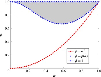
. We find that the viscous flow nonlinear stability region given by (3.48) is a subregion of the inviscid linear stability region (see the
 ${\it\beta}$
versus
 ${\it\alpha}$
diagram in figure 1). The viscous flow nonlinear stability of the circular Couette flow is a global stability result. Inside this stability region, any finite-amplitude axisymmetric perturbation whose initial total circulation function
 $K(x,y,t=0)=K^{C}(y)+\tilde{K}(x,y,t=0)$
satisfies
 $K_{min}^{C}\leqslant K(x,y,t=0)\leqslant K_{max}^{C}$
decays monotonically in time to zero, and the eventual reappearance of the steady circular Couette base flow determined uniquely by the motion of the inner and outer cylinders’ walls is assured (provided that the perturbed flow remains axisymmetric for all times
 $t\geqslant 0$
).
The viscous flow nonlinear stability region for the circular Couette flow:
 $p({\it\alpha})\leqslant {\it\beta}\leqslant 1$
. Also shown for reference is the inviscid flow linear stability region for the circular Couette flow by Rayleigh’s (Reference Rayleigh1916) criterion:
 ${\it\alpha}^{2}<{\it\beta}$
.

3.5.2 An extension of the basic nonlinear stability criterion
In this section, we show that the restriction on the initial total circulation function
 $K(x,y,t=0)$
such that
 $K_{min}^{C}\leqslant K(x,y,t=0)\leqslant K_{max}^{C}$
is not necessary. There are two cases to consider.
(i) Case 1: for
 $B=0$
. This particular circular Couette flow is the solid-body rotation flow within the region
 $V$
. In this case, the difference of the reduced Arnol’d function
 ${\rm\Delta}\mathscr{A}_{rd}$
(given by (3.8)) simplifies to the kinetic energy integral of the perturbation. Hence, we have
 $$\begin{eqnarray}\displaystyle {\rm\Delta}\mathscr{A}_{rd}=\tilde{\mathscr{E}}=\frac{1}{2}{\it\rho}\int _{V}(\tilde{u} _{r}^{2}+\tilde{u} _{x}^{2}+\tilde{u} _{{\it\theta}}^{2})\,\text{d}V. & & \displaystyle\end{eqnarray}$$
Furthermore, the condition (3.37) is trivially satisfied, where the convexity estimates are given by
 ${\it\lambda}^{-}={\it\lambda}^{+}=1>0$
. As a result, in the case when
 $B=0$
, the circular Couette flow is nonlinearly stable to any finite-amplitude axisymmetric perturbation with no additional restrictions.
(ii) Case 2: for
 $B>0$
. In this case, we note that
 $j(K)$
is an analytic function for
 $K>B$
and becomes singular only at
 $K=B$
. If the initial total circulation function satisfies
 $K(x,y,t=0)>B$
, then this would also ensure that the total circulation function
 $K(x,y,t)$
is greater than
 $B$
and remains within the analytic domain of
 $j(K)$
for all times
 $t\geqslant 0$
(due to a maximum principle in appendix C). Thus, the basic formula (3.25) holds. Consequently (under the current restriction on the initial total circulation function), the derivation of Criterion 3.2 is still valid up to (3.46) (prior to the restriction on
 $K_{min}$
to be
 $K_{min}^{C}$
). Let
 $\bar{K}_{min}$
be the minimum value of the initial total circulation function
 $K(x,y,t=0)$
such that (3.46) holds. Then
 $\bar{K}_{min}$
must satisfy
 $$\begin{eqnarray}\displaystyle {\textstyle \frac{1}{3}}ABR_{2}^{2}\leqslant (\bar{K}_{min}-B)^{2}. & & \displaystyle\end{eqnarray}$$
We also consider the case when the restriction on the minimum total circulation value is allowed to be extended below the minimum circulation value of the base flow
 $K_{min}^{C}$
, i.e.
 $\bar{K}_{min}=K_{min}^{C}-{\rm\Delta}K$
with
 ${\rm\Delta}K\geqslant 0$
. Then, (3.50) yields an upper bound for
 ${\rm\Delta}K$
given by
 $$\begin{eqnarray}\displaystyle 0\leqslant {\rm\Delta}K\leqslant AR_{1}^{2}-\sqrt{{\textstyle \frac{1}{3}}ABR_{2}^{2}}<K_{min}^{C}. & & \displaystyle\end{eqnarray}$$
In terms of the non-dimensional parameters
 ${\it\alpha}=R_{1}/R_{2}$
and
 ${\it\beta}={\it\omega}_{2}/{\it\omega}_{1}$
, this upper bound for
 ${\rm\Delta}K$
can be written as
 $$\begin{eqnarray}\displaystyle AR_{1}^{2}-\sqrt{{\textstyle \frac{1}{3}}ABR_{2}^{2}}={\it\omega}_{1}R_{1}^{2}q({\it\alpha},{\it\beta}), & & \displaystyle\end{eqnarray}$$
where
 $q({\it\alpha},{\it\beta})$
is given by
 $$\begin{eqnarray}\displaystyle q({\it\alpha},{\it\beta})=\left(\frac{{\it\beta}-{\it\alpha}^{2}}{1-{\it\alpha}^{2}}\right)-\frac{1}{{\it\alpha}}\sqrt{\frac{1}{3}\left(\frac{{\it\beta}-{\it\alpha}^{2}}{1-{\it\alpha}^{2}}\right)\left(\frac{1-{\it\beta}}{1-{\it\alpha}^{2}}\right)}. & & \displaystyle\end{eqnarray}$$
Rescaling
 ${\rm\Delta}K$
with the minimum circulation value of the base flow
 $K_{min}^{C}={\it\omega}_{1}R_{1}^{2}$
gives
 $$\begin{eqnarray}\displaystyle 0\leqslant \frac{{\rm\Delta}K}{{\it\omega}_{1}R_{1}^{2}}=\frac{{\rm\Delta}K}{K_{min}^{C}}\leqslant q({\it\alpha},{\it\beta}). & & \displaystyle\end{eqnarray}$$
For a given value of the ratio
 ${\rm\Delta}K/K_{min}^{C}$
, we can determine the modified nonlinear stability borderline
 ${\it\beta}_{{\rm\Delta}K/K_{min}^{C}}({\it\alpha})$
for which
 $q({\it\alpha},{\it\beta})={\rm\Delta}K/K_{min}^{C}$
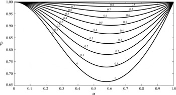
. For various values of the ratio
 ${\rm\Delta}K/K_{min}^{C}$
from 0 to 100 %, the corresponding modified stability regions
 ${\it\beta}_{{\rm\Delta}K/K_{min}^{C}}({\it\alpha})\leqslant {\it\beta}<1$
on the
 ${\it\alpha}$
versus
 ${\it\beta}$
plane are displayed in figure 2. It can be seen that the nonlinear stability region decreases as this ratio increases and is completely eliminated when
 ${\rm\Delta}K/K_{min}^{C}=1$
(which can never occur unless
 $B=0$
).
We also determine the convexity estimates
 ${\it\lambda}^{-}$
and
 ${\it\lambda}^{+}$
used in the energy estimate (3.38) for the extended initial perturbation domain on the total circulation function given by
 $\bar{K}_{min}\leqslant K(x,y,t=0)\leqslant \bar{K}_{max}$
, where
 $\bar{K}_{min}\in [B+\sqrt{ABR_{2}^{2}/3},K_{min}^{C}]$
(determined by rearranging (3.50)) and
 $\bar{K}_{max}\in [K_{max}^{C},\infty )$
. The quantity
 $\bar{K}_{max}$
represents the maximum value of the initial total circulation function
 $K(x,y,t=0)$
such that (3.46) holds, and since
 $K_{max}$
does not appear in (3.46), hence there is no upper limit on
 $\bar{K}_{max}$
.
Once the parameters of the circular Couette flow are given, then the intervals for
 $\bar{K}_{min}$
and
 $\bar{K}_{max}$
are fixed. By specifying the values of
 $\bar{K}_{min}$
and
 $\bar{K}_{max}$
from their respective intervals, then the modified stability region is given by (3.50). The corresponding convexity estimates
 ${\it\lambda}^{-}$
and
 ${\it\lambda}^{+}$
are
 $$\begin{eqnarray}\displaystyle \left.\begin{array}{@{}c@{}}\displaystyle {\it\lambda}^{-}=\min _{\substack{ y_{1}\leqslant y\leqslant y_{2} \\ \bar{K}_{min}\leqslant K\rfloor _{{\it\xi}}\leqslant \bar{K}_{max}}}1+2y\frac{AB}{(K\rfloor _{{\it\xi}}-B)^{2}}=1+\frac{ABR_{1}^{2}}{(\bar{K}_{max}-B)^{2}},\\ \displaystyle {\it\lambda}^{+}=\max _{\substack{ y_{1}\leqslant y\leqslant y_{2} \\ \bar{K}_{min}\leqslant K\rfloor _{{\it\xi}}\leqslant \bar{K}_{max}}}1+2y\frac{AB}{(K\rfloor _{{\it\xi}}-B)^{2}}=1+\frac{ABR_{2}^{2}}{(\bar{K}_{min}-B)^{2}},\end{array}\right\} & & \displaystyle\end{eqnarray}$$
which is an extension of (3.10) with
 $j^{\prime \prime }(K)=AB/(K-B)^{2}$
.
The condition
 $0<{\it\lambda}^{-}<{\it\lambda}^{+}<\infty$
is satisfied without any further reductions in size of the modified stability region. Furthermore, the initial radial and axial velocity perturbations can be as general as possible with no additional restrictions. In the case when
 $\bar{K}_{min}=K_{min}^{C}$
and
 $\bar{K}_{max}=K_{max}^{C}$
, this then recovers the same result as shown in Criterion 3.2.
The nonlinear stability regions (when
 $B>0$
) with respect to any finite-amplitude axisymmetric perturbation whose initial total circulation function satisfies
 $K_{min}^{C}-{\rm\Delta}K\leqslant K(x,y,t=0)<\infty$
for various levels in terms of
 ${\rm\Delta}K/K_{min}^{C}$
, where
 ${\rm\Delta}K\in [0,AR_{1}^{2}-\sqrt{ABR_{2}^{2}/3}]$
.

4 Discussion
In this section we clarify the significance of the present results with respect to the available experimental data by Wendt (Reference Wendt1933) and to the classical studies by Serrin (Reference Serrin1959) and Joseph & Hung (Reference Joseph and Hung1971).
4.1 Experimental evidence for nonlinear stability of the circular Couette flow
Wendt (Reference Wendt1933) conducted a large number of experiments on circular Couette flows and obtained the torque that is required to rotate the cylinders for a general combination of speeds of the two coaxial rotating cylinders. Wendt’s results for the case
 ${\it\alpha}=R_{1}/R_{2}=0.8503$
were summarized in figure 1 by Coles (Reference Coles1965), which is reproduced here in figure 3.
Stability of laminar circular Couette flow. This figure is a graphical representation of a large number of experiments by Wendt (Reference Wendt1933). Here
 ${\it\alpha}=R_{1}/R_{2}=0.8503$
. It is a reproduction of figure 1 in Coles (Reference Coles1965).

In this figure,
 $R_{i}={\it\omega}_{1}R_{1}^{2}/{\it\nu}$
is the Reynolds number based on the inner cylinder’s angular speed of rotation and its radius (
 $0\leqslant R_{i}<12\times 10^{4}$
), and
 $R_{o}={\it\omega}_{2}R_{2}^{2}/{\it\nu}$
is the Reynolds number based on the outer cylinder’s angular speed of rotation and its radius (
 $-16\times 10^{4}\leqslant R_{o}<16\times 10^{4}$
). Note that
 $R_{i}$
and
 $R_{o}$
are independent of each other, and that the two cylinders rotate in opposite directions when
 $R_{o}<0$
. The vertical axis to both the
 $R_{i}$
and
 $R_{o}$
axes represents the ratio of the measured torque
 $M$
, needed to rotate the two cylinders over the theoretical torque
 $M_{lam}$
, computed according to the laminar circular Couette flow solution. When the torque ratio equals one, it indicates that the base circular Couette flow is established with no perturbation and the base flow is (nonlinearly) stable to finite-amplitude perturbations. However, when the torque ratio is greater than one, it indicates that the base circular Couette flow develops finite-amplitude perturbations, and a higher torque is needed to rotate the cylinders and overcome the additional resistance caused by the perturbations. This means that the base circular Couette flow is unstable in such situations.
It is seen from figure 3 that the inviscid flow linear neutral stability line, given by the ray
 ${\it\omega}_{1}R_{1}^{2}={\it\omega}_{2}R_{2}^{2}$
(or
 $R_{i}=R_{o}$
, which was constructed from a potential (inviscid) flow analysis of axisymmetric infinitesimally small perturbations), determines the existence of a (nonlinear) stable region of operation for a viscous circular Couette flow in the range
 $0<R_{i}<R_{o}$
, specifically at high-Reynolds-number situations (say
 $R_{o}>10\,000$
). The case of a solid-body rotation flow for which
 ${\it\omega}_{1}={\it\omega}_{2}$
(i.e.
 $R_{i}={\it\alpha}^{2}R_{o}$
) is included within the stable region. We also note that, when
 $R_{i}$
is low and
 $R_{o}>10^{5}$
, there is another region of operation with changes from the base flow.
The inviscid flow linear neutral stability line correctly predicts the change of the base circular Couette flow stability. However, its scope is limited to infinitesimal perturbations and, as such, does not guarantee flow stability in the range
 $0<R_{i}<R_{o}$
in response to finite-amplitude perturbations. The present results provide the sufficient operational conditions (3.48) for the axisymmetric viscous flow nonlinear stability of the base circular Couette flow, which in terms of
 $R_{i}$
and
 $R_{o}$
become
 $$\begin{eqnarray}\displaystyle {\it\alpha}^{2}R_{o}<R_{i}<\frac{{\it\alpha}^{2}}{p({\it\alpha})}R_{o}. & & \displaystyle\end{eqnarray}$$
The current nonlinear stability borderlines according to (4.1) are shown in figure 4(a,b) for the set-up with
 ${\it\alpha}=0.8503$
. Also shown is the inviscid flow linear neutral stability line of Rayleigh (Reference Rayleigh1916) for this set-up,
 $R_{i}=R_{o}$
. It can be seen that the present nonlinear stability region of operation is within the linear stability region for all
 $R_{o}>0$
. In addition, figure 4 also shows the classical results by Serrin (Reference Serrin1959). We note that, within the scale of figure 4(a), the current lower nonlinear stability line
 $R_{i}={\it\alpha}^{2}R_{o}$
(which is also the solid-body rotation line) closely coincides with Serrin’s (Reference Serrin1959) two nonlinear stability lines. However, in the scale of figure 4(b), which focuses on lower Reynolds numbers
 $R_{i}$
and
 $R_{o}$
in the range between
 $0$
and
 $10\,000$
, the differences between these lines become more apparent.
The stability results by Serrin (Reference Serrin1959) and Joseph & Hung (Reference Joseph and Hung1971) are discussed in the following subsections (§§ 4.2.1 and 4.2.2).
The axisymmetric nonlinear stability region (the grey area) for
 ${\it\alpha}=R_{1}/R_{2}=0.8503$
(
 $R_{\tilde{\mathscr{E}}}=1563.24$
) (or
 ${\it\alpha}^{-1}=1.176$
as used in the experiment by Wendt (Reference Wendt1933)) in the range (a)
 $0\leqslant R_{o}<160\,000$
and (b)
 $0\leqslant R_{o}<10\,000$
.

4.2 Discussion of the classical nonlinear stability results
4.2.1 Serrin’s (Reference Serrin1959) nonlinear stability result
It is well known that a solid-body rotation flow between two coaxial rotating cylinders is globally stable with a monotonic decay of the perturbation’s kinetic energy in time. In the case when the circular Couette flow is near a solid-body rotation (when
 $B$
is close to zero), it is expected that the flow is also globally stable with a monotonic decay of the perturbation’s kinetic energy in time. To explore this idea, Serrin (Reference Serrin1959) developed an energy stability analysis, which used the perturbation’s kinetic energy integral defined by
 $$\begin{eqnarray}\displaystyle \tilde{\mathscr{E}}=\frac{1}{2}{\it\rho}\int _{V}(\tilde{u} _{r}^{2}+\tilde{u} _{x}^{2}+\tilde{u} _{{\it\theta}}^{2})\,\text{d}V & & \displaystyle\end{eqnarray}$$
as a Lyapunov function. His analysis was essentially based on the Reynolds–Orr equation, which relates the rate of change in time of
 $\tilde{\mathscr{E}}$
to the exchange of energy in the bulk with the base flow (which is determined by the base flow strain-rate tensor) and also the energy dissipation due to viscous effects (see also Wu, Ma & Zhou Reference Wu, Ma and Zhou2006), i.e.
 $$\begin{eqnarray}\displaystyle \frac{\text{d}\tilde{\mathscr{E}}}{\text{d}t}={\it\rho}B\int _{V}\frac{\tilde{u} _{r}\tilde{u} _{{\it\theta}}}{y}\,\text{d}V-{\it\mu}\int _{V}\left(\frac{\tilde{u} _{r}^{2}}{2y}+\frac{\tilde{u} _{{\it\theta}}^{2}}{2y}+|\boldsymbol{{\rm\nabla}}\tilde{u} _{r}|^{2}+|\boldsymbol{{\rm\nabla}}\tilde{u} _{x}|^{2}+|\boldsymbol{{\rm\nabla}}\tilde{u} _{{\it\theta}}|^{2}\right)\text{d}V. & & \displaystyle\end{eqnarray}$$
Serrin (Reference Serrin1959) estimated the various terms in (4.3) and established the inequality
 $$\begin{eqnarray}\displaystyle \frac{\text{d}\tilde{\mathscr{E}}}{\text{d}t}\leqslant -{\it\rho}({\it\nu}-{\it\nu}_{\tilde{\mathscr{E}}})\int _{V}\left(\frac{\tilde{u} _{r}^{2}}{2y}+\frac{\tilde{u} _{{\it\theta}}^{2}}{2y}+|\boldsymbol{{\rm\nabla}}\tilde{u} _{r}|^{2}+|\boldsymbol{{\rm\nabla}}\tilde{u} _{x}|^{2}+|\boldsymbol{{\rm\nabla}}\tilde{u} _{{\it\theta}}|^{2}\right)\text{d}V, & & \displaystyle\end{eqnarray}$$
where the constant
 ${\it\nu}_{\mathscr{\tilde{E}}}$
is the critical viscosity level found from the variational problem,
 $$\begin{eqnarray}\displaystyle {\it\nu}_{\mathscr{\tilde{E}}}=\frac{|B|}{R_{\mathscr{\tilde{E}}}}=\max {\displaystyle \frac{|B|\displaystyle \int _{V}\frac{\tilde{u} _{r}\tilde{u} _{{\it\theta}}}{y}\,\text{d}V}{\displaystyle \int _{V}\left(\frac{\tilde{u} _{r}^{2}}{2y}+\frac{\tilde{u} _{{\it\theta}}^{2}}{2y}+|\boldsymbol{{\rm\nabla}}\tilde{u} _{r}|^{2}+|\boldsymbol{{\rm\nabla}}\tilde{u} _{x}|^{2}+|\boldsymbol{{\rm\nabla}}\tilde{u} _{{\it\theta}}|^{2}\right)\text{d}V}}. & & \displaystyle\end{eqnarray}$$
In this process of maximization,
 $\tilde{\boldsymbol{u}}=(\tilde{u} _{r},\tilde{u} _{x},\tilde{u} _{{\it\theta}})$
is searched among all admissible initial perturbation fields to maximize
 ${\it\nu}_{\mathscr{\tilde{E}}}$
, i.e. among all axisymmetric functions that vanish at the cylinders’ walls and satisfy axial periodic boundary conditions. From (4.4), the kinetic energy integral of the perturbation
 $\tilde{\mathscr{E}}$
decays monotonically in time when
 $|B|<{\it\nu}R_{\mathscr{\tilde{E}}}$
. According to Serrin (Reference Serrin1959), the stability region determined by (4.4) and (4.5) is a constant band centred around the solid-body rotation line
 $R_{i}={\it\alpha}^{2}R_{o}$
and is given by
 $$\begin{eqnarray}\displaystyle {\it\alpha}^{2}R_{o}-R_{\mathscr{\tilde{E}}}(1-{\it\alpha}^{2})<R_{i}<{\it\alpha}^{2}R_{o}+R_{\mathscr{\tilde{E}}}(1-{\it\alpha}^{2}), & & \displaystyle\end{eqnarray}$$
where the value
 $R_{\mathscr{\tilde{E}}}=|B|/{\it\nu}_{\mathscr{\tilde{E}}}$
is determined by (4.5). In the particular case when the cylinders are close to each other, the consequential eigenvalue problem from (4.5) can be well approximated by a simpler set of ordinary differential equations. We have
 $R_{\mathscr{\tilde{E}}}=41.2{\it\alpha}/(1-{\it\alpha})^{2}$
(see Serrin Reference Serrin1959, for details). Using this result for the set-up with
 ${\it\alpha}=0.8503$
, it is found that
 $R_{\mathscr{\tilde{E}}}=1563.24$
and
 $R_{\mathscr{\tilde{E}}}(1-{\it\alpha}^{2})=433.00$
.
The global nonlinear stability region according to Serrin (Reference Serrin1959) is significant when the operational Reynolds numbers are small (see figure 4
b). However, at high Reynolds numbers, it only forms a narrow band of operational conditions around the solid-body rotation flow set-up. The region of nonlinear stability (4.6) around the solid-body rotation line is relatively small and cannot even be seen in the large scales of
 $R_{i}$
and
 $R_{o}$
that were studied in the experiments (see figure 4
a). Furthermore, in order for the circular Couette base flow to be within the stability band in the case of high Reynolds numbers, the parameter
 $B$
must be sufficiently close to zero. This represents the class of circular Couette base flows that are very close to a solid-body rotation flow, hence it must be susceptible to any finite-amplitude perturbation. In the general case when the parameter
 $B$
is not sufficiently close to zero, then the viscosity of the fluid
 ${\it\nu}$
is required to be greater than a certain level (determined by
 ${\it\nu}_{\mathscr{\tilde{E}}}$
in (4.5)) in order to establish nonlinear stability. As a result, Serrin’s (Reference Serrin1959) classical nonlinear stability analysis is effective in the study of viscous rotating flows that have low Reynolds numbers.
4.2.2 Joseph & Hung’s (Reference Joseph and Hung1971) nonlinear stability result
Synge (Reference Synge1938a
,Reference Synge
b
) established the stability of the circular Couette flow for
 $A>0$
and
 $B>0$
in response to axisymmetric perturbations within the analysis of linear stability theory. Joseph & Hung’s (Reference Joseph and Hung1971) nonlinear stability result is a nonlinear extension of Synge’s linear result (Synge Reference Synge1938a
,Reference Synge
b
). In their approach, a weighted perturbation’s kinetic energy integral, which has exactly the same form as
 $\tilde{\mathscr{E}}_{w}$
defined by (3.35), was used as a Lyapunov function. They derived a formula for the rate of change in time of
 $\tilde{\mathscr{E}}_{w}$
that is similar to the linearized estimate (3.36), i.e.
 $$\begin{eqnarray}\displaystyle \frac{\text{d}\tilde{\mathscr{E}}_{w}}{\text{d}t}=-{\it\rho}\frac{B}{A}\int _{V}\frac{\tilde{u} _{{\it\theta}}^{2}\tilde{u} _{r}}{\sqrt{2}y^{3/2}}\,\text{d}V-{\it\mu}\mathscr{D}, & & \displaystyle\end{eqnarray}$$
where
 $$\begin{eqnarray}\displaystyle \mathscr{D}=\int _{V}\left(\frac{\tilde{u} _{r}^{2}}{2y}+|\boldsymbol{{\rm\nabla}}\tilde{u} _{r}|^{2}+|\boldsymbol{{\rm\nabla}}\tilde{u} _{x}|^{2}\!+\left(1+\frac{B}{2Ay}\right)\left[\left(\frac{\partial \tilde{u} _{{\it\theta}}}{\partial x}\right)^{2}+\left(\sqrt{2y}\frac{\partial \tilde{u} _{{\it\theta}}}{\partial y}-\frac{\tilde{u} _{{\it\theta}}}{\sqrt{2y}}\right)^{2}\right]\right)\text{d}V. & & \displaystyle \nonumber\\ \displaystyle & & \displaystyle\end{eqnarray}$$
The formula (4.7) is valid for the nonlinear dynamics of perturbations on the base flow. However, there is one difference in (4.7) with respect to (3.36), which is the appearance of the first integral in (4.7) (containing
 $\tilde{u} _{{\it\theta}}^{2}\tilde{u} _{r}/\sqrt{2}y^{3/2}$
as the integrand). This term reflects the nonlinear inviscid flow interaction between the perturbation’s velocity components
 $\tilde{u} _{r}$
and
 $\tilde{u} _{{\it\theta}}$
. In terms of the perturbation’s amplitude, this nonlinear term is of cubic order and may be neglected when the perturbation is sufficiently small. However, when the perturbation’s amplitude is large, then this nonlinear term must be carefully studied. It can be shown that this nonlinear term can be bounded from above by the following set of inequalities:
 $$\begin{eqnarray}\displaystyle \!\!\!\int _{V}\left|\frac{\tilde{u} _{{\it\theta}}^{2}\tilde{u} _{r}}{\sqrt{2}y^{3/2}}\right|\text{d}V & {\leqslant} & \displaystyle \frac{1}{\sqrt{2}y_{1}^{3/2}}\int _{V}|\tilde{u} _{{\it\theta}}^{2}\tilde{u} _{r}|\,\text{d}V\leqslant \frac{1}{\sqrt{2}y_{1}^{3/2}}\left(\int _{V}|\tilde{u} _{{\it\theta}}|^{4}\,\text{d}V\right)^{1/2}\left(\int _{V}|\tilde{u} _{r}|^{2}\,\text{d}V\right)^{1/2}\nonumber\\ \displaystyle & {\leqslant} & \displaystyle \frac{M_{1}}{\sqrt{2}y_{1}^{3/2}}\left(\int _{V}|\boldsymbol{{\rm\nabla}}\tilde{u} _{{\it\theta}}|^{2}\,\text{d}V\right)\left(\int _{V}|\tilde{u} _{r}|^{2}\,\text{d}V\right)^{1/2}\leqslant \frac{M_{1}}{y_{1}^{3/2}}\mathscr{D}\left(\frac{\tilde{\mathscr{E}}_{w}}{{\it\rho}}\right)^{1/2}\!.\end{eqnarray}$$
The constant
 $M_{1}$
is given by the Sobolev inequality (see e.g. Adams & Fournier Reference Adams and Fournier2003), which can be found by the minimization process
 $$\begin{eqnarray}\displaystyle M_{1}=\left[\min {\displaystyle \frac{\displaystyle \int _{V}|\boldsymbol{{\rm\nabla}}\tilde{u} _{{\it\theta}}|^{2}\,\text{d}V}{\displaystyle \left(\int _{V}\tilde{u} _{{\it\theta}}^{4}\,\text{d}V\right)^{1/2}}}\right]^{-1}. & & \displaystyle\end{eqnarray}$$
In this minimization process,
 $\tilde{u} _{{\it\theta}}$
is searched among all admissible initial perturbation fields to minimize
 $M_{1}$
(i.e. among all axisymmetric functions that vanish at the cylinders’ walls and satisfy axial periodic boundary conditions). Inserting (4.9) into (4.7) gives
 $$\begin{eqnarray}\displaystyle \frac{\text{d}\tilde{\mathscr{E}}_{w}}{\text{d}t}=-{\it\rho}\frac{B}{A}\int _{V}\frac{\tilde{u} _{{\it\theta}}^{2}\tilde{u} _{r}}{\sqrt{2}y^{3/2}}\,\text{d}V-{\it\mu}\mathscr{D}\leqslant -\left({\it\mu}-{\it\rho}\frac{|B|M_{1}}{Ay_{1}^{3/2}}\left(\frac{\tilde{\mathscr{E}}_{w}}{{\it\rho}}\right)^{1/2}\right)\mathscr{D}. & & \displaystyle\end{eqnarray}$$
It is clear that, when the size of the initial weighted perturbation’s kinetic energy integral
 $\tilde{\mathscr{E}}_{w0}$
satisfies
 $$\begin{eqnarray}\displaystyle \left(\frac{\tilde{\mathscr{E}}_{w0}}{{\it\rho}}\right)^{1/2}\leqslant {\it\nu}\frac{Ay_{1}^{3/2}}{|B|M_{1}}, & & \displaystyle\end{eqnarray}$$
then
 $\text{d}\tilde{\mathscr{E}}_{w}/\text{d}t\leqslant 0$
, and thus
 $\tilde{\mathscr{E}}_{w}$
decays monotonically in time.
Therefore, the condition for nonlinear stability of the circular Couette flow according to Joseph & Hung (Reference Joseph and Hung1971) is
 $A>0$
or
 $R_{i}<R_{o}$
, i.e. this is Rayleigh’s (Reference Rayleigh1916) inviscid linear stability criterion (see figure 4).
It is remarkable that, in the case
 $A>0$
, Joseph & Hung’s (Reference Joseph and Hung1971) analysis shows that inviscid flow linear stability also implies local nonlinear stability of the viscous flow with respect to finite but sufficiently small initial perturbations as dictated by (4.12), where the upper bound on the initial weighted perturbation’s kinetic energy integral is not global and is always limited by the viscosity level of the fluid.
In terms of the base flow parameters, the upper bound on the initial weighted perturbation’s kinetic energy integral (4.12) for a fixed value of
 $A>0$
increases when either the fluid viscosity
 ${\it\nu}$
increases or the value of
 $|B|$
decreases, and decreases when either the fluid viscosity
 ${\it\nu}$
decreases or the value of
 $|B|$
increases. This is as expected, since the case
 $B=0$
represents the solid-body rotation flow (which is globally and monotonically stable in response to any finite-amplitude perturbation). In terms of Reynolds numbers, for a fixed value of
 $R_{o}$
, the upper bound on the initial weighted perturbation’s kinetic energy integral (4.12) decreases in value when
 $R_{i}$
increases from
 ${\it\alpha}^{2}R_{o}$
to
 $R_{o}$
or when
 $R_{i}$
decreases from
 ${\it\alpha}^{2}R_{o}$
to
 $0$
.
In the case for viscous circular Couette flows with a high Reynolds number, the upper bound on the initial weighted perturbation’s kinetic energy integral (4.12) can be severely limited. This is due to the limitation of (4.7), where the conservation of
 $\tilde{\mathscr{E}}_{w}$
only holds in the linearized inviscid dynamics and leaves the high-order nonlinear dynamics in its primitive form. However, this can be compensated in the special case when the parameter
 $B$
of the circular Couette flow is sufficiently close to zero. This represents the class of circular Couette flows that are very close to a solid-body rotation flow, hence the upper bound on the initial weighted perturbation’s kinetic energy integral (4.12) is of an applicable size. In the general case when
 $B$
is not sufficiently close to zero, the viscosity of the fluid must be sufficiently high in order for the upper bound on the initial weighted perturbation’s kinetic energy integral (4.12) to have a realistic value. As a result, Joseph & Hung’s (Reference Joseph and Hung1971) classical nonlinear stability analysis is effective in the study of viscous circular Couette flows that have low Reynolds numbers, where viscous stresses can dissipate large finite-amplitude perturbations.
4.3 The current nonlinear stability result
In the current approach to the nonlinear stability of the base viscous circular Couette flow, all the inviscid interactions between the perturbations of the various velocity components are accounted for in the difference of the reduced Arnol’d function
 ${\rm\Delta}\mathscr{A}_{rd}$
given by (3.8). This leads to the fact that the weighted perturbation’s kinetic energy integral, given by
 $\tilde{\mathscr{E}}\rfloor _{{\it\xi}}={\rm\Delta}\mathscr{A}_{rd}$
, is an invariant physical quantity in the inviscid-limit flow (see Wang Reference Wang2009). It is important to note that the special choice of
 $j(K)$
(as defined in (3.7)) and also the application of the mean value theorem in the second-order Taylor’s expansion enable
 ${\rm\Delta}\mathscr{A}_{rd}$
to be rewritten as the weighted perturbation’s kinetic energy integral
 $\tilde{\mathscr{E}}\rfloor _{{\it\xi}}$
, and hence to be used as a Lyapunov function.
The current viscous flow nonlinear stability analysis of the circular Couette flow is built upon estimating the rate of change in time of
 $\tilde{\mathscr{E}}\rfloor _{{\it\xi}}$
rather than its linearized form (3.35), which was used in Joseph & Hung (Reference Joseph and Hung1971) (for the study of axisymmetric nonlinear dynamics of perturbations) and in Kloosterziel (Reference Kloosterziel2010) (for the study of axisymmetric linearized dynamics of perturbations). Therefore, the resulting formula for
 $\text{d}\tilde{\mathscr{E}}\rfloor _{{\it\xi}}/\text{d}t$
given by (3.25) does not contain any inviscid flow nonlinear terms, specifically not the inviscid flow nonlinear terms that appear according to Serrin (Reference Serrin1959) in (4.3) or according to Joseph & Hung (Reference Joseph and Hung1971) in (4.7). As a result, the present nonlinear stability criterion is derived from the inequalities (3.29) and (3.30) (see § 3.5 for finer details), and the size of the perturbations is independent of the fluid viscosity.
The significance of this present nonlinear stability result is that the stable region of operation presented in figure 1 depends only on the set-up of the system, which is independent of the fluid viscosity. Moreover, this nonlinear stability result is of a global nature, which is valid for any initial finite-amplitude axisymmetric perturbation (except for a minor restriction on the initial total circulation function
 $K(x,y,t=0)$
). This result also extends and strengthens the classical results by Serrin (Reference Serrin1959) and Joseph & Hung (Reference Joseph and Hung1971). Note that our predicted nonlinear stability region shown in figure 4 covers a finite stable operational region that was revealed in Wendt’s (Reference Wendt1933) experiments, whereas Serrin’s (Reference Serrin1959) result only provides a small, fixed, stable band around the solid-body rotation line, which is negligible for high values of
 $R_{o}$
.
5 Examples
In the following examples, we further study the cases of a solid-body rotation flow and of a specific set-up of the circular Couette flow and develop for both cases their respective analytical upper-bound estimates for the decay rate of an axisymmetric finite-amplitude perturbation.
5.1 Solid-body rotation flow between two coaxial rotating cylinders
For a solid-body rotation flow with
 ${\it\omega}_{1}={\it\omega}_{2}={\it\omega}$
(i.e.
 ${\it\beta}=1$
) between two coaxial rotating cylinders with radii
 $R_{1}$
and
 $R_{2}$
(
 $0<{\it\alpha}=R_{1}/R_{2}<1$
), we find from (3.8) that in this special case of
 ${\it\beta}=1$
we have
 ${\rm\Delta}\mathscr{A}_{rd}=\tilde{\mathscr{E}}$
. From (3.25), we have the identity (since
 $B=0$
)
 $$\begin{eqnarray}\displaystyle \frac{\text{d}\tilde{\mathscr{E}}}{\text{d}t}=-{\it\mu}\int _{V}\left(\frac{\tilde{u} _{r}^{2}}{2y}+\frac{\tilde{u} _{{\it\theta}}^{2}}{2y}+|\boldsymbol{{\rm\nabla}}\tilde{u} _{r}|^{2}+|\boldsymbol{{\rm\nabla}}\tilde{u} _{x}|^{2}+|\boldsymbol{{\rm\nabla}}\tilde{u} _{{\it\theta}}|^{2}\right)\text{d}V. & & \displaystyle\end{eqnarray}$$
The identity (5.1) shows that any initial axisymmetric finite-amplitude perturbation around the solid-body rotation flow decays in time. By using the Sobolev inequality (Adams & Fournier Reference Adams and Fournier2003), and the boundary conditions that all the velocity perturbations vanish at the wall, we have
 $$\begin{eqnarray}\displaystyle \int _{V}(\tilde{u} _{r}^{2}+\tilde{u} _{x}^{2}+\tilde{u} _{{\it\theta}}^{2})\,\text{d}V\leqslant M_{2}\int _{V}(|\boldsymbol{{\rm\nabla}}\tilde{u} _{r}|^{2}+|\boldsymbol{{\rm\nabla}}\tilde{u} _{x}|^{2}+|\boldsymbol{{\rm\nabla}}\tilde{u} _{{\it\theta}}|^{2})\,\text{d}V, & & \displaystyle\end{eqnarray}$$
where
 $M_{2}>0$
is a constant determined by the size of the cylinders. The constant
 $M_{2}$
is estimated from the minimization process
 $$\begin{eqnarray}\displaystyle M_{2}=\left[\min {\displaystyle \frac{\displaystyle \int _{V}|\boldsymbol{{\rm\nabla}}\tilde{u} |^{2}\,\text{d}V}{\displaystyle \int _{V}\tilde{u} ^{2}\,\text{d}V}}\right]^{-1}. & & \displaystyle\end{eqnarray}$$
In this process of minimization,
 $\tilde{u}$
is searched among all the admissible initial perturbation fields to minimize
 $M_{2}$
. As a result, we can bound the right-hand side of (5.1) and find that
 $$\begin{eqnarray}\displaystyle \frac{\text{d}\tilde{\mathscr{E}}}{\text{d}t}\leqslant -\frac{2{\it\nu}}{M_{2}}\tilde{\mathscr{E}}. & & \displaystyle\end{eqnarray}$$
This yields the following analytical upper-bound estimate for the decay of the perturbation’s kinetic energy integral
 $\tilde{\mathscr{E}}$
:
 $$\begin{eqnarray}\displaystyle \tilde{\mathscr{E}}(t)\leqslant \tilde{\mathscr{E}}_{0}\text{e}^{-2{\it\nu}t/M_{2}}, & & \displaystyle\end{eqnarray}$$
for all times
 $t\geqslant 0$
.
For two circular coaxial rotating cylinders with inner and outer wall radii
 $R_{1}$
and
 $R_{2}$
, respectively,
 $M_{2}$
can be found from
 $M_{2}=R_{2}^{2}/{\it\lambda}_{1}$
, where
 ${\it\lambda}_{1}$
is the first eigenvalue of the problem
 $$\begin{eqnarray}\displaystyle {\rm\Delta}w(r^{\dagger })+{\it\lambda}w(r^{\dagger })=0\quad \left({\rm\Delta}w=w_{r^{\dagger }r^{\dagger }}+\frac{w_{r^{\dagger }}}{r^{\dagger }}\right) & & \displaystyle\end{eqnarray}$$
on the annulus
 ${\it\alpha}=R_{1}/R_{2}<r^{\dagger }=r/R_{2}<1$
with Dirichlet conditions
 $w({\it\alpha})=0$
and
 $w(1)=0$
. The general solution of this eigenvalue problem is a linear combination of Bessel functions,
 $$\begin{eqnarray}\displaystyle w(r^{\dagger })=C_{1}\text{J}_{0}(\sqrt{{\it\lambda}}r^{\dagger })+C_{2}\text{Y}_{0}(\sqrt{{\it\lambda}}r^{\dagger }), & & \displaystyle\end{eqnarray}$$
where
 $\text{J}_{0}$
and
 $\text{Y}_{0}$
are the Bessel functions of the first and second kind of order
 $m=0$
. Applying the boundary conditions yields the following characteristic equation:
 $$\begin{eqnarray}\displaystyle \text{J}_{0}(\sqrt{{\it\lambda}})\text{Y}_{0}(\sqrt{{\it\lambda}}{\it\alpha})-\text{Y}_{0}(\sqrt{{\it\lambda}})\text{J}_{0}(\sqrt{{\it\lambda}}{\it\alpha})=0. & & \displaystyle\end{eqnarray}$$
The solution of the first eigenvalue
 ${\it\lambda}_{1}$
of (5.6) (or the first zero of (5.8)) for various values of
 ${\it\alpha}$
in the range between
 $0.1$
and
 $0.8$
is shown in figure 5. It can be seen that
 ${\it\lambda}_{1}$
increases with
 ${\it\alpha}$
. The analytical upper bound for the perturbation’s decay rate is then estimated by
 ${\it\sigma}_{E}^{\ast }=-2{\it\lambda}_{1}{\it\nu}/R_{2}^{2}$
. This upper bound (for the decay rate) is independent of the angular speed of rotation
 ${\it\omega}$
. Rescaling the time such that
 $t^{\ast }={\it\omega}t$
and by using
 $R_{o}={\it\omega}R_{2}^{2}/{\it\nu}$
, we can also rewrite it as
 ${\it\sigma}_{E}^{\ast }=-2{\it\lambda}_{1}/R_{o}$
. We find that, as the gap between the cylinders becomes smaller (
 ${\it\alpha}$
increases towards
 $1$
), the flow perturbation decays faster in time, while, as the Reynolds number of the outer cylinder
 $R_{o}$
increases, the perturbation decays slower in time. In addition, for a fixed rate of rotation of the cylinders (including the case of no rotation) or for cylinders with an accelerating rotational speed from zero up to a given value and then rotation is stopped, the perturbation’s decay rate is approximately the same as this analytical upper-bound estimate as long as the flow stays axisymmetric.
The dependence of
 ${\it\lambda}_{1}$
on
 ${\it\alpha}$
.

To further elaborate on the perturbation’s dynamics, we focus on the example where
 ${\it\alpha}=0.5$
and then
 ${\it\lambda}_{1}=39.0138$
. This leads to
 $$\begin{eqnarray}\displaystyle \tilde{\mathscr{E}}(t)\leqslant \tilde{\mathscr{E}}_{0}\text{e}^{-2{\it\nu}t/M_{2}}\approx \tilde{\mathscr{E}}_{0}\text{e}^{-78.0276t^{\ast }/R_{o}}. & & \displaystyle\end{eqnarray}$$
In this case, the upper bound for the decay rate of the perturbation’s kinetic energy integral
 $\tilde{\mathscr{E}}$
is estimated by
 ${\it\sigma}_{E}^{\ast }=-78.0276/R_{o}$
.
We also conducted numerical simulations of the flow dynamics based on (2.3), (2.4a
) and (2.4b
) and the assumed boundary conditions. These simulations are based on a modified code of Rusak et al. (Reference Rusak, Wang, Xu and Taylor2012) and Rusak, Granata & Wang (Reference Rusak, Granata and Wang2015), which includes the viscous terms and axial periodic boundary conditions. For the case of a base flow with
 ${\it\beta}=1$
and
 $0<{\it\alpha}<1$
, we used various initial conditions given by
 $$\begin{eqnarray}\displaystyle \left.\begin{array}{@{}c@{}}\displaystyle {\it\psi}(x,y,0)={\it\epsilon}_{{\it\psi}}\cos \left(\frac{2{\rm\pi}nx}{L}\right)f(y),\\ \displaystyle {\it\chi}(x,y,0)=-{\it\epsilon}_{{\it\chi}}\cos \left(\frac{2{\rm\pi}nx}{L}\right)\left[f_{yy}(y)-\left(\frac{2{\rm\pi}n}{L}\right)^{2}\frac{f(y)}{2y}\right],\\ \displaystyle K(x,y,0)=2{\it\omega}y-{\it\epsilon}_{K}\cos \left(\frac{2{\rm\pi}nx}{L}\right)f(y),\end{array}\right\} & & \displaystyle\end{eqnarray}$$
for
 $0\leqslant x<L$
and
 $y_{1}\leqslant y\leqslant y_{2}$
, where
 ${\it\epsilon}_{{\it\psi}},{\it\epsilon}_{{\it\chi}}$
and
 ${\it\epsilon}_{K}$
are the perturbation’s amplitudes. The constant
 $n$
is an integer, and
 $f(y)=(y-y_{1})^{2}(y_{2}-y)^{2}/c_{m}$
(
 $c_{m}$
is a scaling factor such that
 $\max f(y)=1$
).
The numerical simulations of the evolution for the non-dimensional perturbation’s kinetic energy integral
 $\tilde{\mathscr{E}}^{non}=\tilde{\mathscr{E}}/({\it\rho}{\it\omega}_{2}^{2}R_{2}^{2})$
with
 $R_{o}=100$
,
 ${\it\alpha}=0.5$
,
 ${\it\beta}=1$
,
 ${\it\omega}=1$
,
 $L=2$
,
 $R_{2}=1$
and various initial conditions according to (5.10) (with
 $c_{m}=0.001236$
) are presented in figure 6. The initial non-dimensional perturbation’s kinetic energy integral
 $\tilde{\mathscr{E}}^{non}|_{t=0}=0.000242$
is the same for all cases shown. Also shown for reference is the analytic upper bound for the decay of the perturbation’s kinetic energy integral
 $\tilde{\mathscr{E}}$
according to the right-hand side of (5.9) (the heavy solid line). It can be seen that the case with
 ${\it\epsilon}_{{\it\psi}}={\it\epsilon}_{{\it\chi}}=0$
,
 ${\it\epsilon}_{K}=0.01236$
and
 $n=0$
shows a decay of
 $\tilde{\mathscr{E}}$
(the curve using open circles) that is only slightly below this predicted analytical upper bound (the heavy solid line). In all other cases with various
 ${\it\epsilon}_{{\it\psi}}$
,
 ${\it\epsilon}_{{\it\chi}}$
,
 ${\it\epsilon}_{K}$
and
 $n$
,
 $\tilde{\mathscr{E}}$
decays faster than this analytic upper-bound prediction. The decay process for each of these perturbations involves a stage of nonlinear interaction between the flow perturbations that enhances the flow mixing and increases the decay of the perturbations. The numerical simulations demonstrate that this analytic upper-bound decay line provides a simple and relevant criterion for all the processes.
The computed time history of the non-dimensional perturbation’s kinetic energy integral
 $\tilde{\mathscr{E}}^{non}=\tilde{\mathscr{E}}/({\it\rho}{\it\omega}_{2}^{2}R_{2}^{2})$
for
 $R_{o}=100$
,
 ${\it\alpha}=0.5$
,
 ${\it\beta}=1$
,
 ${\it\omega}=1$
,
 $L=2$
,
 $R_{2}=1$
for various initial conditions. All perturbations start with the same initial value of
 $\tilde{\mathscr{E}}^{non}|_{t=0}=0.000242$
. The heavy solid line is the analytic upper bound for the decay of the perturbation’s kinetic energy integral
 $\tilde{\mathscr{E}}$
according to (5.9). The other curves are for the following cases: open circles,
 ${\it\epsilon}_{{\it\psi}}={\it\epsilon}_{{\it\chi}}=0$
,
 ${\it\epsilon}_{K}=0.01236$
and
 $n=0$
; open squares,
 ${\it\epsilon}_{{\it\psi}}={\it\epsilon}_{{\it\chi}}=0$
,
 ${\it\epsilon}_{K}=0.01748$
and
 $n=1$
; open diamonds,
 ${\it\epsilon}_{{\it\psi}}={\it\epsilon}_{{\it\chi}}=0$
,
 ${\it\epsilon}_{K}=0.01748$
and
 $n=2$
; open downward-pointing triangles,
 ${\it\epsilon}_{{\it\psi}}={\it\epsilon}_{{\it\chi}}=0.00058$
,
 ${\it\epsilon}_{K}=0.01164$
and
 $n=0$
; open upward-pointing triangles,
 ${\it\epsilon}_{{\it\psi}}={\it\epsilon}_{{\it\chi}}=0.00082$
,
 ${\it\epsilon}_{K}=0.01626$
and
 $n=1$
; open left-pointing triangles,
 ${\it\epsilon}_{{\it\psi}}={\it\epsilon}_{{\it\chi}}=0.00223$
,
 ${\it\epsilon}_{K}=0$
and
 $n=1$
; dotted line,
 ${\it\epsilon}_{{\it\psi}}={\it\epsilon}_{{\it\chi}}=0.00172$
,
 ${\it\epsilon}_{K}=0$
and
 $n=0$
.

5.2 Circular Couette flow
We analyse the circular Couette flow for various parameters
 $0<{\it\alpha}<1$
and
 $0<{\it\beta}<1$
. The analytical upper-bound estimate for the decay rate of
 ${\rm\Delta}\mathscr{A}_{rd}$
is derived directly from (3.25). To this end, we first evaluate the term on the left-hand side of (3.46) when
 $K_{min}=K_{min}^{C}$
, and then rewrite it in terms of the non-dimensional parameters
 ${\it\alpha}$
and
 ${\it\beta}$
. This yields
 $$\begin{eqnarray}\displaystyle d({\it\alpha},{\it\beta})=1-\frac{ABR_{2}^{2}}{3(K_{min}-B)^{2}}=1-\frac{(1-{\it\beta})}{3({\it\beta}-{\it\alpha}^{2}){\it\alpha}^{2}}. & & \displaystyle\end{eqnarray}$$
Thus from (3.25), we have the following upper bound for the temporal rate of change of
 ${\rm\Delta}\mathscr{A}_{rd}$
:
 $$\begin{eqnarray}\displaystyle \frac{\text{d}{\rm\Delta}\mathscr{A}_{rd}}{\text{d}t}\leqslant -{\it\mu}\int _{V}(|\boldsymbol{{\rm\nabla}}\tilde{u} _{r}|^{2}+|\boldsymbol{{\rm\nabla}}\tilde{u} _{x}|^{2}+d({\it\alpha},{\it\beta})|\boldsymbol{{\rm\nabla}}\tilde{u} _{{\it\theta}}|^{2})\,\text{d}V, & & \displaystyle\end{eqnarray}$$
which is valid for any initial finite-amplitude axisymmetric perturbation such that
 $K_{min}^{C}\leqslant K(x,y,t=0)\leqslant K_{max}^{C}$
.
Using the Sobolev inequality (Adams & Fournier Reference Adams and Fournier2003), this leads to
 $$\begin{eqnarray}\displaystyle \frac{\text{d}{\rm\Delta}\mathscr{A}_{rd}}{\text{d}t}\leqslant -\frac{{\it\mu}}{M_{2}}\int _{V}(\tilde{u} _{r}^{2}+\tilde{u} _{x}^{2}+d({\it\alpha},{\it\beta})\tilde{u} _{{\it\theta}}^{2})\,\text{d}V. & & \displaystyle\end{eqnarray}$$
The constant
 $M_{2}$
can be found again from
 $M_{2}=R_{2}^{2}/{\it\lambda}_{1}$
, where
 ${\it\lambda}_{1}$
is the same exact first eigenvalue found in § 5.1 and is a function of
 ${\it\alpha}$
alone (see figure 5). On the other hand, we also have from (3.8) and (3.10) that
 $$\begin{eqnarray}\displaystyle 0<{\rm\Delta}\mathscr{A}_{rd}\leqslant \frac{1}{2}{\it\rho}\int _{V}(\tilde{u} _{r}^{2}+\tilde{u} _{x}^{2}+{\it\lambda}^{+}({\it\alpha},{\it\beta})\tilde{u} _{{\it\theta}}^{2})\,\text{d}V. & & \displaystyle\end{eqnarray}$$
Combining (5.13) and (5.14) gives
 $$\begin{eqnarray}\displaystyle \frac{\text{d}{\rm\Delta}\mathscr{A}_{rd}}{\text{d}t}\leqslant -\frac{d({\it\alpha},{\it\beta})}{{\it\lambda}^{+}({\it\alpha},{\it\beta})}\frac{2{\it\nu}}{M_{2}}{\rm\Delta}\mathscr{A}_{rd}. & & \displaystyle\end{eqnarray}$$
Thus, we have
 $$\begin{eqnarray}\displaystyle {\rm\Delta}\mathscr{A}_{rd}(t)\leqslant {\rm\Delta}\mathscr{A}_{rd0}\exp \left(-\frac{d({\it\alpha},{\it\beta})}{{\it\lambda}^{+}({\it\alpha},{\it\beta})}\frac{2{\it\nu}}{M_{2}}t\right) & & \displaystyle\end{eqnarray}$$
and
 $$\begin{eqnarray}\displaystyle \Vert \tilde{\boldsymbol{u}}(t)\Vert _{{\it\lambda}^{-}}^{2} & := & \displaystyle \frac{1}{2}{\it\rho}\int _{V}(\tilde{u} _{r}^{2}+\tilde{u} _{x}^{2}+{\it\lambda}^{-}({\it\alpha},{\it\beta})\tilde{u} _{{\it\theta}}^{2})\,\text{d}V\nonumber\\ \displaystyle & {\leqslant} & \displaystyle \exp \left(-\frac{d({\it\alpha},{\it\beta})}{{\it\lambda}^{+}({\it\alpha},{\it\beta})}\frac{2{\it\nu}}{M_{2}}t\right)\frac{1}{2}{\it\rho}\int _{V}(\tilde{u} _{r0}^{2}+\tilde{u} _{x0}^{2}+{\it\lambda}^{+}({\it\alpha},{\it\beta})\tilde{u} _{{\it\theta}0}^{2})\,\text{d}V\nonumber\\ \displaystyle & = & \displaystyle \exp \left(-\frac{d({\it\alpha},{\it\beta})}{{\it\lambda}^{+}({\it\alpha},{\it\beta})}\frac{2{\it\nu}}{M_{2}}t\right)\Vert \tilde{\boldsymbol{u}}(t=0)\Vert _{{\it\lambda}^{+}}^{2}.\end{eqnarray}$$
We find that the perturbation
 $\tilde{\boldsymbol{u}}=(\tilde{u} _{r},\tilde{u} _{x},\tilde{u} _{{\it\theta}})$
at a later time in terms of the stability norm
 $\Vert \cdot \Vert _{{\it\lambda}^{-}}^{2}$
given by the perturbation’s weighted kinetic energy integral (as defined by the left-hand side of (5.17)) is bounded from above by the initial perturbation
 $\tilde{\boldsymbol{u}}_{0}=(\tilde{u} _{r0},\tilde{u} _{x0},\tilde{u} _{{\it\theta}0})$
in terms of the stability norm
 $\Vert \cdot \Vert _{{\it\lambda}^{+}}^{2}$
given by the perturbation’s weighted kinetic energy integral (as defined by the right-hand side of (5.17)). The upper bound for the decay rate of the perturbation’s weighted kinetic energy integral is estimated analytically by
 ${\it\sigma}_{WE}^{\ast }=-2{\it\lambda}_{1}({\it\alpha})(d({\it\alpha},{\it\beta})/{\it\lambda}^{+}({\it\alpha},{\it\beta}))({\it\nu}/R_{2}^{2})$
. Rescaling the time
 $t$
such that
 $t^{\ast }={\it\omega}_{2}t$
and using the Reynolds number based on the outer cylinder
 $R_{o}={\it\omega}_{2}R_{2}^{2}/{\it\nu}$
, we can write
 ${\it\sigma}_{WE}^{\ast }=-2{\it\lambda}_{1}({\it\alpha})(d({\it\alpha},{\it\beta})/{\it\lambda}^{+}({\it\alpha},{\it\beta}))(1/R_{o})$
. This upper bound depends on
 ${\it\alpha}$
(the geometry of the cylinders),
 ${\it\beta}$
(the ratio of the rates of rotation of the cylinders) and
 $R_{o}$
(the Reynolds number of the outer cylinder).
The computed time history of the non-dimensional perturbation’s weighted kinetic energy integral
 $\tilde{\mathscr{E}}_{{\it\lambda}^{-}}^{non}=\Vert \tilde{\boldsymbol{u}}(t)\Vert _{{\it\lambda}^{-}}^{2}/({\it\rho}{\it\omega}_{2}^{2}R_{2}^{2})$
for
 $R_{o}=100$
,
 ${\it\alpha}=0.8$
,
 ${\it\beta}=0.96$
,
 ${\it\omega}_{2}=1$
,
 $L=2$
,
 $R_{2}=1$
and various initial conditions. All perturbations start with the same initial value, which is given by the initial weighted kinetic energy integral
 $\tilde{\mathscr{E}}_{{\it\lambda}^{+}}^{non}|_{t=0}=0.00021$
(according to the right-hand side of (5.18)). The heavy solid line is the analytic upper bound for the decay of perturbation according to (5.18). The other curves are for the following cases: open circles,
 ${\it\epsilon}_{{\it\psi}}={\it\epsilon}_{{\it\chi}}=0$
,
 ${\it\epsilon}_{K}=0.01755$
and
 $n=0$
; open squares,
 ${\it\epsilon}_{{\it\psi}}={\it\epsilon}_{{\it\chi}}=0$
,
 ${\it\epsilon}_{K}=0.02482$
and
 $n=1$
; open diamonds,
 ${\it\epsilon}_{{\it\psi}}={\it\epsilon}_{{\it\chi}}=0$
,
 ${\it\epsilon}_{K}=0.02482$
and
 $n=2$
; open downward-pointing triangles,
 ${\it\epsilon}_{{\it\psi}}={\it\epsilon}_{{\it\chi}}=0.00067$
,
 ${\it\epsilon}_{K}=0.01410$
and
 $n=0$
; open upward-pointing triangles,
 ${\it\epsilon}_{{\it\psi}}={\it\epsilon}_{{\it\chi}}=0.00092$
,
 ${\it\epsilon}_{K}=0.02000$
and
 $n=1$
; open left-pointing triangles,
 ${\it\epsilon}_{{\it\psi}}={\it\epsilon}_{{\it\chi}}=0.00155$
,
 ${\it\epsilon}_{K}=0$
and
 $n=1$
; dotted line,
 ${\it\epsilon}_{{\it\psi}}={\it\epsilon}_{{\it\chi}}=0.00111$
,
 ${\it\epsilon}_{K}=0$
and
 $n=0$
.

For the case with
 ${\it\alpha}=R_{1}/R_{2}=0.8$
and
 ${\it\beta}={\it\omega}_{2}/{\it\omega}_{1}=0.96$
, the computation gives that
 ${\it\lambda}_{1}=246.4298$
,
 ${\it\lambda}^{-}=1.0512$
,
 ${\it\lambda}^{+}=1.1953$
and
 $d=0.9349$
. Then, (5.17) becomes
 $$\begin{eqnarray}\displaystyle \frac{1}{2}{\it\rho}\int _{V}(\tilde{u} _{r}^{2}+\tilde{u} _{x}^{2}+1.0512\tilde{u} _{{\it\theta}}^{2})\,\text{d}V\leqslant \text{e}^{-385.49t^{\ast }/R_{o}}\frac{1}{2}{\it\rho}\int _{V}(\tilde{u} _{r0}^{2}+\tilde{u} _{x0}^{2}+1.1953\tilde{u} _{{\it\theta}0}^{2})\,\text{d}V.\quad & & \displaystyle\end{eqnarray}$$
The upper bound for the decay rate of the perturbation’s weighted kinetic energy integral is estimated analytically by
 ${\it\sigma}_{WE}^{\ast }=-385.49/R_{o}$
.
Numerical simulation results of the evolution of the non-dimensional perturbation’s weighted kinetic energy integral
 $\tilde{\mathscr{E}}_{{\it\lambda}^{-}}^{non}=\Vert \tilde{\boldsymbol{u}}(t)\Vert _{{\it\lambda}^{-}}^{2}/({\it\rho}{\it\omega}_{2}^{2}R_{2}^{2})$
according to the left-hand side of (5.18) for
 $R_{o}=100$
,
 ${\it\alpha}=0.8$
,
 ${\it\beta}=0.96$
,
 ${\it\omega}_{2}=1$
,
 $L=2$
,
 $R_{2}=1$
and various initial conditions similar to those in (5.10) (with
 $c_{m}=0.000066$
) are presented in figure 7. The initial non-dimensional perturbation’s weighted kinetic energy integral
 $\tilde{\mathscr{E}}_{{\it\lambda}^{+}}^{non}|_{t=0}$
according to the right-hand side of (5.18) is the same for all cases shown, which equals
 $0.00021$
. Also shown for reference is the analytic upper-bound line for the decay of the perturbation (the heavy solid line) according to the right-hand side of (5.18). It can be seen that the case with
 ${\it\epsilon}_{{\it\psi}}={\it\epsilon}_{{\it\chi}}=0$
,
 ${\it\epsilon}_{K}=0.01755$
and
 $n=0$
shows a decay of the non-dimensional perturbation’s weighted kinetic energy integral (the curve with open circles) that is below this predicted analytic upper bound (the heavy solid line). In all other cases studied, the non-dimensional perturbation’s weighted kinetic energy integral decays faster than this upper-bound prediction. Again, each of these decay processes involves a stage of nonlinear interaction between the flow perturbations that enhances the flow mixing and increases the decay of the perturbations. The numerical simulations demonstrate that this analytic upper-bound decay line provides a simple and relevant criterion for all the processes.
6 Conclusion
An extension to the classical sufficient conditions for the nonlinear stability of the circular Couette flow in response to axisymmetric finite-amplitude perturbations under axial periodic boundary conditions is developed through a novel rigorous analysis. This analysis is based on investigating the difference of the reduced Arnol’d function from its base flow value (given by
 ${\rm\Delta}\mathscr{A}_{rd}:=\mathscr{A}_{rd}({\it\chi},K)-\mathscr{A}_{rd}({\it\chi}^{C},K^{C})$
). It is through a specific choice for the function
 $j(K)$
in the formulation of
 $\mathscr{C}_{S}$
and also the application of the mean value theorem in the second-order Taylor’s expansion that enable this difference to be rewritten as a weighted kinetic energy integral of the perturbation
 $\tilde{\mathscr{E}}\rfloor _{{\it\xi}}$
, and hence to be used as a Lyapunov function. We show that all the inviscid flow effects as well as all the viscous-dependent terms that are related to the flow boundaries vanish. As a result, the evolution of
 ${\rm\Delta}\mathscr{A}_{rd}=\tilde{\mathscr{E}}\rfloor _{{\it\xi}}$
depends only on the viscous effects of the perturbation’s dynamics in the bulk. The requirement for the temporal decay of this function for all time leads to two novel sufficient conditions (3.29) and (3.30), for the axisymmetric nonlinear stability of the circular Couette flow (given the existence of positive finite value convexity estimates). The linearized version of these conditions for infinitesimally small perturbations recovers the recent linear stability results by Kloosterziel (Reference Kloosterziel2010). We derive conditions for the axisymmetric nonlinear stability, and also establish a definite stability region in terms of operational parameters for the circular Couette flow, where the flow is nonlinearly stable to any initial axisymmetric finite-amplitude perturbation as long as the initial total circulation function satisfies the condition
 $K(x,y,t=0)\geqslant B+\sqrt{ABR_{2}^{2}/3}$
(see details in figure 1 and also in figure 2). In particular, this nonlinear stability region is independent of the fluid viscosity. Our results are in agreement with the classical experiments by Wendt (Reference Wendt1933), and also extend the classical nonlinear stability results by Serrin (Reference Serrin1959) and Joseph & Hung (Reference Joseph and Hung1971) (see the detailed discussion in § 4).
We also develop an energy estimate in terms of the perturbation’s weighted kinetic energy integral given by (3.38) with (3.39), which characterizes the limit of the growth of transient perturbation modes. Finally, we derive analytical estimates for the upper bound on the decay rate of axisymmetric finite-amplitude viscous perturbations to the solid-body rotation flow between two coaxial rotating cylinders and to the circular Couette flow (see the results in § 5). Extensive numerical simulations demonstrate that this analytical upper bound is relevant to the dynamics of various axisymmetric perturbations tested, where it is strictly obeyed (see the computed examples in figures 6 and 7).
This present analysis reveals the stability mechanism of the circular Couette flow, through the Arnol’d energy-Casimir formulation, in terms of the exchange of kinetic energy between the base flow, the perturbation and the cylinders’ walls, including the effects of viscous diffusion in the bulk, and also the viscous wall stresses. When the sufficient conditions for nonlinear stability are satisfied by the base flow, then this mechanism leads to the monotonic temporal decay of any suitable axisymmetric perturbations and keeps the perturbed flow in the neighbourhood of the steady circular Couette flow state. Under such conditions, the eventual realization of the unique standard circular Couette flow determined by the coaxial rotating cylinders is guaranteed (provided that the perturbed flow stays axisymmetric for all time). This mechanism is rigorously proven and provides useful quantitative upper-bound estimates on the perturbations’ decay rate, which can be used as benchmark test cases in the study of viscous flows between rotating cylinders and also in the development of direct numerical simulation codes for viscous flow dynamics.
This present study is limited to the nonlinear stability of the circular Couette flow in response to finite-amplitude axisymmetric perturbations. The experiments of Wendt (Reference Wendt1933) and Andereck et al. (Reference Andereck, Liu and Swinney1986) show that, in the identified nonlinear stability region, the flow is stable to all perturbations (including any axisymmetric and three-dimensional perturbation). However, finite-amplitude three-dimensional perturbations may appear in flows that are outside this nonlinear stability region, specifically when the pipes are counter-rotating. In such states, the flow may develop spiral wave states, intermittencies and further transits into various turbulent states as the inner cylinder’s Reynolds number
 $R_{i}$
is increased at a fixed value of the outer cylinder’s Reynolds number
 $R_{o}$
(see details in figure 1 of Andereck et al. (Reference Andereck, Liu and Swinney1986)).
Appendix A. Derivation of Identity 3.1
Proof. To derive Identity 3.1, we use the axisymmetric viscous flow equations (2.1a
)–(2.1d
), the no-penetration and the no-slip conditions along the inner
 $(r=R_{1})$
and outer
 $(r=R_{2})$
cylinders’ walls, and the axial periodic boundary conditions at
 $x=0$
and
 $x=L$
. The direct computation of
 $\text{d}\mathscr{E}/\text{d}t$
followed by the application of integration by parts shows that all the inviscid flow terms vanish (as found in § 3.1). The resulting formula for the temporal rate of change of the total kinetic energy integral
 $\mathscr{E}$
is given by the viscous effects only:
 $$\begin{eqnarray}\displaystyle \frac{\text{d}\mathscr{E}}{\text{d}t}=4{\rm\pi}{\it\mu}\int _{0}^{L}\left[yu_{{\it\theta}}^{C}\frac{\partial u_{{\it\theta}}}{\partial y}\right]_{y=y_{1}}^{y=y_{2}}\,\text{d}x-{\it\mu}\int _{V}\left(\frac{u_{r}^{2}}{2y}+\frac{u_{{\it\theta}}^{2}}{2y}+|\boldsymbol{{\rm\nabla}}u_{r}|^{2}+|\boldsymbol{{\rm\nabla}}u_{{\it\theta}}|^{2}+|\boldsymbol{{\rm\nabla}}u_{x}|^{2}\right)\text{d}V. & & \displaystyle \nonumber\\ \displaystyle & & \displaystyle\end{eqnarray}$$
Equation (A 1) represents the balance of energy of the axisymmetric flow in the domain
 $V$
. The first integral describes the total work done on the flow by the viscous stresses at the inner and outer walls and the second integral describes the energy damping in the bulk by viscosity.
Inserting
 $u_{r}=\tilde{u} _{r}$
,
 $u_{x}=\tilde{u} _{x}$
and
 $u_{{\it\theta}}=u_{{\it\theta}}^{C}(y)+\tilde{u} _{{\it\theta}}$
into (A 1) results in
 $$\begin{eqnarray}\displaystyle \frac{\text{d}\mathscr{E}}{\text{d}t} & = & \displaystyle 4{\rm\pi}{\it\mu}\int _{0}^{L}\left[yu_{{\it\theta}}^{C}\frac{\text{d}u_{{\it\theta}}^{C}}{\text{d}y}\right]_{y=y_{1}}^{y=y_{2}}\,\text{d}x-{\it\mu}\int _{V}\left(\frac{u_{{\it\theta}}^{C2}}{2y}+|\boldsymbol{{\rm\nabla}}u_{{\it\theta}}^{C}|^{2}\right)\text{d}V\nonumber\\ \displaystyle & & \displaystyle +\,4{\rm\pi}{\it\mu}\int _{0}^{L}\left[yu_{{\it\theta}}^{C}\frac{\partial \tilde{u} _{{\it\theta}}}{\partial y}\right]_{y=y_{1}}^{y=y_{2}}\text{d}x-{\it\mu}\int _{V}\left(\frac{\tilde{u} _{r}^{2}}{2y}+\frac{\tilde{u} _{{\it\theta}}^{2}}{2y}+|\boldsymbol{{\rm\nabla}}\tilde{u} _{r}|^{2}+|\boldsymbol{{\rm\nabla}}\tilde{u} _{{\it\theta}}|^{2}+|\boldsymbol{{\rm\nabla}}\tilde{u} _{x}|^{2}\right)\text{d}V\nonumber\\ \displaystyle & & \displaystyle -\,{\it\mu}\int _{V}\left(\frac{u_{{\it\theta}}^{C}\tilde{u} _{{\it\theta}}}{y}+2\boldsymbol{{\rm\nabla}}u_{{\it\theta}}^{C}\boldsymbol{\cdot }\boldsymbol{{\rm\nabla}}\tilde{u} _{{\it\theta}}\right)\text{d}V.\end{eqnarray}$$
The first term presents the net work done on the base flow by viscous stresses along the cylindrical walls. The second term describes the energy damping on the base flow in the bulk by viscosity. The sum of these two terms vanishes for any steady base columnar rotating flow. The last term can be integrated by parts, which shows
 $$\begin{eqnarray}\displaystyle \int _{V}\left(\frac{u_{{\it\theta}}^{C}\tilde{u} _{{\it\theta}}}{y}+2\boldsymbol{{\rm\nabla}}u_{{\it\theta}}^{C}\boldsymbol{\cdot }\boldsymbol{{\rm\nabla}}\tilde{u} _{{\it\theta}}\right)\text{d}V=\int _{V}\left(\frac{u_{{\it\theta}}^{C}}{y}-2{\rm\Delta}u_{{\it\theta}}^{C}\right)\tilde{u} _{{\it\theta}}\,\text{d}V=0. & & \displaystyle\end{eqnarray}$$
The right-hand side of (A 3) vanishes for any steady axisymmetric viscous columnar rotating flow. The identity (3.11) results from (A 2), (A 3) and definitions (3.12) and (3.13).☐
Appendix B. Derivation of Identity 3.2
Proof. To derive Identity 3.2, we use (2.4a
) of the Squire–Long system of equations, the no-penetration and the no-slip conditions along the inner
 $(r=R_{1})$
and outer
 $(r=R_{2})$
cylinders’ walls, and the axial periodic boundary conditions at
 $x=0$
and
 $x=L$
. The direct computation of
 $\text{d}\mathscr{C}_{S}/\text{d}t$
followed by the application of integration by parts shows that all the inviscid flow terms vanish (as found in § 3.1). The resulting formula for the temporal rate of change of the circulation-dependent integral (Casimir’s integral)
 $\mathscr{C}_{S}$
is given by the viscous effects only:
 $$\begin{eqnarray}\displaystyle \frac{\text{d}\mathscr{C}_{S}}{\text{d}t}={\it\mu}\int _{V}j^{\prime }(K)\left(\frac{\partial ^{2}K}{\partial x^{2}}+2y\frac{\partial ^{2}K}{\partial y^{2}}\right)\text{d}V. & & \displaystyle\end{eqnarray}$$
The integration of (B 1) by parts gives
 $$\begin{eqnarray}\displaystyle \frac{\text{d}\mathscr{C}_{S}}{\text{d}t} & = & \displaystyle 2{\rm\pi}{\it\mu}\int _{y_{1}}^{y_{2}}\left(\left[j^{\prime }(K)\frac{\partial K}{\partial x}\right]_{x=0}^{x=L}-\int _{0}^{L}\frac{\partial }{\partial x}(j^{\prime }(K))\frac{\partial K}{\partial x}\,\text{d}x\right)\text{d}y\nonumber\\ \displaystyle & & \displaystyle +\,4{\rm\pi}{\it\mu}\int _{0}^{L}\left(\left[yj^{\prime }(K)\frac{\partial K}{\partial y}\right]_{y=y_{1}}^{y=y_{2}}-\int _{y_{1}}^{y_{2}}\frac{\partial }{\partial y}(yj^{\prime }(K))\frac{\partial K}{\partial y}\,\text{d}y\right)\text{d}x.\end{eqnarray}$$
Then by using the axial periodic boundary conditions and further simplifications, we obtain
 $$\begin{eqnarray}\displaystyle \frac{\text{d}\mathscr{C}_{S}}{\text{d}t} & = & \displaystyle 4{\rm\pi}{\it\mu}\int _{0}^{L}\left[yj^{\prime }(K)\frac{\partial K}{\partial y}\right]_{y=y_{1}}^{y=y_{2}}\text{d}x-4{\rm\pi}{\it\mu}\int _{D}\frac{\partial }{\partial y}(j(K))\,\text{d}D\nonumber\\ \displaystyle & & \displaystyle -\,{\it\mu}\int _{V}j^{\prime \prime }(K)\left(\frac{\partial K}{\partial x}\right)^{2}\text{d}V-2{\it\mu}\int _{V}yj^{\prime \prime }(K)\left(\frac{\partial K}{\partial y}\right)^{2}\text{d}V.\end{eqnarray}$$
Inserting
 $K=K^{C}(y)+\tilde{K}$
into (B 3), then each individual integral of (B 3) is estimated separately. In estimating the first term of (B 3), using the no-slip conditions for the circulation perturbation
 $\tilde{K}(x,y=y_{1},t)=\tilde{K}(x,y=y_{2},t)=0$
along the cylinders’ walls gives
 $$\begin{eqnarray}\displaystyle \int _{0}^{L}\left[yj^{\prime }(K)\frac{\partial K}{\partial y}\right]_{y=y_{1}}^{y=y_{2}}\text{d}x=\int _{0}^{L}\left[yj^{\prime }(K^{C})\frac{\text{d}K^{C}}{\text{d}y}\right]_{y=y_{1}}^{y=y_{2}}\text{d}x+\int _{0}^{L}\left[yj^{\prime }(K^{C})\frac{\partial \tilde{K}}{\partial y}\right]_{y=y_{1}}^{y=y_{2}}\text{d}x. & & \displaystyle\end{eqnarray}$$
In estimating the second term of (B 3), we conduct an integration along
 $y$
and find that
 $$\begin{eqnarray}\displaystyle \int _{D}\frac{\partial }{\partial y}(j(K))\,\text{d}D=\int _{0}^{L}[j(K^{C})]_{y=y_{1}}^{y=y_{2}}\,\text{d}x. & & \displaystyle\end{eqnarray}$$
In estimating the third term of (B 3), we use the fact that
 $K^{C}$
is
 $x$
-independent and find that
 $$\begin{eqnarray}\displaystyle \int _{V}j^{\prime \prime }(K)\left(\frac{\partial K}{\partial x}\right)^{2}\text{d}V=\int _{V}j^{\prime \prime }(K)\left(\frac{\partial \tilde{K}}{\partial x}\right)^{2}\text{d}V. & & \displaystyle\end{eqnarray}$$
In estimating the fourth term in (B 3), it is necessary to account for the contributions from the two terms
 $j^{\prime \prime }(K)$
and
 $(\partial K/\partial y)^{2}$
. To do this, we can first consider it as a function of a single variable
 $s\in \mathbb{R}$
, and then apply the remainder formula of the second-order Taylor’s expansion.
In order to apply the second-order Taylor’s expansion on the fourth term of (B 3), we define a function
 $h(s)$
in terms of a single variable
 $s\in \mathbb{R}$
, which is given by
 $$\begin{eqnarray}\displaystyle h(s)=\int _{V}yj^{\prime \prime }(K^{C}+s\tilde{K})\left(\frac{\text{d}K^{C}}{\text{d}y}+s\frac{\partial \tilde{K}}{\partial y}\right)^{2}\text{d}V. & & \displaystyle\end{eqnarray}$$
Then the second-order Taylor’s expansion of the function
 $h(s)$
around the fixed point
 $s_{0}$
is
 $$\begin{eqnarray}\displaystyle h(s)=h(s_{0})+h^{\prime }(s_{0})(s-s_{0})+\frac{h^{\prime \prime }({\it\zeta})}{2}(s-s_{0})^{2}, & & \displaystyle\end{eqnarray}$$
where
 ${\it\zeta}$
is an intermediate value between
 $s_{0}$
and
 $s$
, that is
 $s_{0}<{\it\zeta}<s$
. By the chain rule, the first and second derivatives of the function
 $h(s)$
are given by
 $$\begin{eqnarray}\displaystyle h^{\prime }(s) & = & \displaystyle \frac{\text{d}}{\text{d}s}\left[\int _{V}yj^{\prime \prime }(K^{C}+s\tilde{K})\left(\frac{\text{d}K^{C}}{\text{d}y}+s\frac{\partial \tilde{K}}{\partial y}\right)^{2}\text{d}V\right]\nonumber\\ \displaystyle & = & \displaystyle \int _{V}\frac{\partial }{\partial s}\left[yj^{\prime \prime }(K^{C}+s\tilde{K})\left(\frac{\text{d}K^{C}}{\text{d}y}+s\frac{\partial \tilde{K}}{\partial y}\right)^{2}\right]\text{d}V\nonumber\\ \displaystyle & = & \displaystyle \int _{V}\left[yj^{\prime \prime \prime }(K^{C}+s\tilde{K})\left(\frac{\text{d}K^{C}}{\text{d}y}+s\frac{\partial \tilde{K}}{\partial y}\right)^{2}\tilde{K}\right.\nonumber\\ \displaystyle & & \displaystyle +\,\left.2yj^{\prime \prime }(K^{C}+s\tilde{K})\left(\frac{\text{d}K^{C}}{\text{d}y}+s\frac{\partial \tilde{K}}{\partial y}\right)\frac{\partial \tilde{K}}{\partial y}\right]\text{d}V,\end{eqnarray}$$
 $$\begin{eqnarray}\displaystyle h^{\prime \prime }(s) & = & \displaystyle \frac{\text{d}^{2}}{\text{d}s^{2}}\left[\int _{V}yj^{\prime \prime }(K^{C}+s\tilde{K})\left(\frac{\text{d}K^{C}}{\text{d}y}+s\frac{\text{d}\tilde{K}}{\partial y}\right)^{2}\text{d}V\right]\nonumber\\ \displaystyle & = & \displaystyle \frac{\text{d}}{\text{d}s}\int _{V}\left[yj^{\prime \prime \prime }(K^{C}+s\tilde{K})\left(\frac{\text{d}K^{C}}{\text{d}y}+s\frac{\partial \tilde{K}}{\partial y}\right)^{2}\tilde{K}\right.\nonumber\\ \displaystyle & & \displaystyle +\,\left.2yj^{\prime \prime }(K^{C}+s\tilde{K})\left(\frac{\text{d}K^{C}}{\text{d}y}+s\frac{\partial \tilde{K}}{\partial y}\right)\frac{\partial \tilde{K}}{\partial y}\right]\text{d}V\nonumber\\ \displaystyle & = & \displaystyle \int _{V}\left[yj^{\prime \prime \prime \prime }(K^{C}+s\tilde{K})\left(\frac{\text{d}K^{C}}{\text{d}y}+s\frac{\partial \tilde{K}}{\partial y}\right)^{2}\tilde{K}^{2}\right.\nonumber\\ \displaystyle & & \displaystyle +\,4yj^{\prime \prime \prime }(K^{C}+s\tilde{K})\left(\frac{\text{d}K^{C}}{\text{d}y}+s\frac{\partial \tilde{K}}{\partial y}\right)\tilde{K}\frac{\partial \tilde{K}}{\partial y}\nonumber\\ \displaystyle & & \displaystyle +\,\left.2yj^{\prime \prime }(K^{C}+s\tilde{K})\left(\frac{\partial \tilde{K}}{\partial y}\right)^{2}\right]\text{d}V.\end{eqnarray}$$
 $s_{0}=0$
and
 $s=1$
back in the second-order Taylor’s expansion of the function
 $h(s)$
(given by (B 8)) yields the remainder formula of the second-order Taylor’s expansion on the fourth term of (B 3) around
 $(K^{C},\text{d}K^{C}/\text{d}y)$
, which is given by
 $$\begin{eqnarray}\displaystyle & & \displaystyle \int _{V}yj^{\prime \prime }(K)\left(\frac{\partial K}{\partial y}\right)^{2}\,\text{d}V=\int _{V}yj^{\prime \prime }(K^{C})\left(\frac{\text{d}K^{C}}{\text{d}y}\right)^{2}\,\text{d}V+\int _{V}yj^{\prime \prime \prime }(K^{C})\left(\frac{\text{d}K^{C}}{\text{d}y}\right)^{2}\tilde{K}\nonumber\\ \displaystyle & & \displaystyle \quad +2yj^{\prime \prime }(K^{C})\frac{\text{d}K^{C}}{\text{d}y}\frac{\partial \tilde{K}}{\partial y}\,\text{d}V+\int _{V}\frac{y}{2}\left[j^{\prime \prime \prime \prime }(K\rfloor _{{\it\zeta}})\left(\left.\frac{\partial K}{\partial y}\right\rfloor _{{\it\zeta}}\right)^{2}\tilde{K}^{2}\right.\nonumber\\ \displaystyle & & \displaystyle \quad \left.+\,4j^{\prime \prime \prime }(K\rfloor _{{\it\zeta}})\left.\frac{\partial K}{\partial y}\right\rfloor _{{\it\zeta}}\tilde{K}\frac{\partial \tilde{K}}{\partial y}+2j^{\prime \prime }(K\rfloor _{{\it\zeta}})\left(\frac{\partial \tilde{K}}{\partial y}\right)^{2}\right]\text{d}V,\end{eqnarray}$$
where the definitions of the intermediate instantaneous functions
 $K\rfloor _{{\it\zeta}}$
and
 $\partial K/\partial y\rfloor _{{\it\zeta}}$
are given by (3.18).
In addition, we also have
 $$\begin{eqnarray}\displaystyle 4{\rm\pi}\int _{0}^{L}\left[yj^{\prime }(K^{C})\frac{\text{d}K^{C}}{\text{d}y}-j(K^{C})\right]_{y=y_{1}}^{y=y_{2}}\text{d}x-2\int _{V}yj^{\prime \prime }(K^{C})\left(\frac{\text{d}K^{C}}{\text{d}y}\right)^{2}\text{d}V=0. & & \displaystyle\end{eqnarray}$$
This is because, for a steady base columnar rotating flow
 $K=K^{C}(y)$
of (2.4a
) and (2.4b
), the summation of the base flow contributions in (B 4), (B 5) and (B 10) must vanish identically. Inserting the results from (B 4)–(B 6) along with (B 10) and (B 11) back into (B 3), together with definitions (3.16) and (3.17), we obtain the identity (3.15).☐
Appendix C. Maximum principle
Proof of (3.45).
Let
 ${\it\sigma}>0$
be a positive constant and set
 $\hat{K}(x,y,t)=\text{e}^{-{\it\sigma}t}K(x,y,t)$
. It is easy to verify that
 $\hat{K}(x,y,t)$
satisfies
 $$\begin{eqnarray}\displaystyle \frac{\partial \hat{K}}{\partial t}+\frac{\partial {\it\psi}}{\partial y}\frac{\partial \hat{K}}{\partial x}-\frac{\partial {\it\psi}}{\partial x}\frac{\partial \hat{K}}{\partial y}={\it\nu}\left(\frac{\partial ^{2}\hat{K}}{\partial x^{2}}+2y\frac{\partial ^{2}\hat{K}}{\partial y^{2}}\right)-{\it\sigma}\hat{K}. & & \displaystyle\end{eqnarray}$$
Now, suppose
 $\hat{K}$
attains a positive maximum value at a point
 $(x^{\circ },y^{\circ },t^{\circ })$
, where
 $(x^{\circ },y^{\circ })$
is an interior point of the domain
 $D$
and
 $t^{\circ }\in (0,T]$
. It is necessary that we have
 $$\begin{eqnarray}\displaystyle \frac{\partial \hat{K}}{\partial t}\geqslant 0,\quad \frac{\partial \hat{K}}{\partial x}=\frac{\partial \hat{K}}{\partial y}=0,\quad \frac{\partial ^{2}\hat{K}}{\partial x^{2}}\leqslant 0\quad \text{and}\quad \frac{\partial ^{2}\hat{K}}{\partial y^{2}}\leqslant 0\quad \text{at}~(x^{\circ },y^{\circ },t^{\circ }). & & \displaystyle\end{eqnarray}$$
But this contradicts (C 1), as the left-hand side of (C 1) is non-negative and the right-hand side of (C 1) is strictly negative. Thus, the positive maximum of
 $\hat{K}$
can only occur at the boundary (and also at
 $t^{\circ }=0$
), which is found as
 $K_{max}$
. Therefore,
 $\text{e}^{-{\it\sigma}t}K(x,y,t)\leqslant K_{max}$
for
 $t\geqslant 0$
. The upper bound of (3.45) is obtained by letting
 ${\it\sigma}\rightarrow 0$
.
Similarly, we can show that a positive minimum of
 $K$
can only occur at the boundary (and also at
 $t^{\circ }=0$
) by considering
 $\hat{K}(x,y,t)=\text{e}^{{\it\sigma}t}K(x,y,t)$
, with
 ${\it\sigma}>0$
and thereby proving the lower bound of (3.45).
Note that, as we have shown that the total circulation function
 $K(x,y,t)$
is bounded below and above by
 $K_{min}=\min K(x,y,t=0)$
and
 $K_{max}=\max K(x,y,t=0)$
for all times
 $t\geqslant 0$
, and since these values are required to be positive by the nonlinear stability criterion, we do not consider the case when the values of
 $K$
are negative.☐