1 Introduction
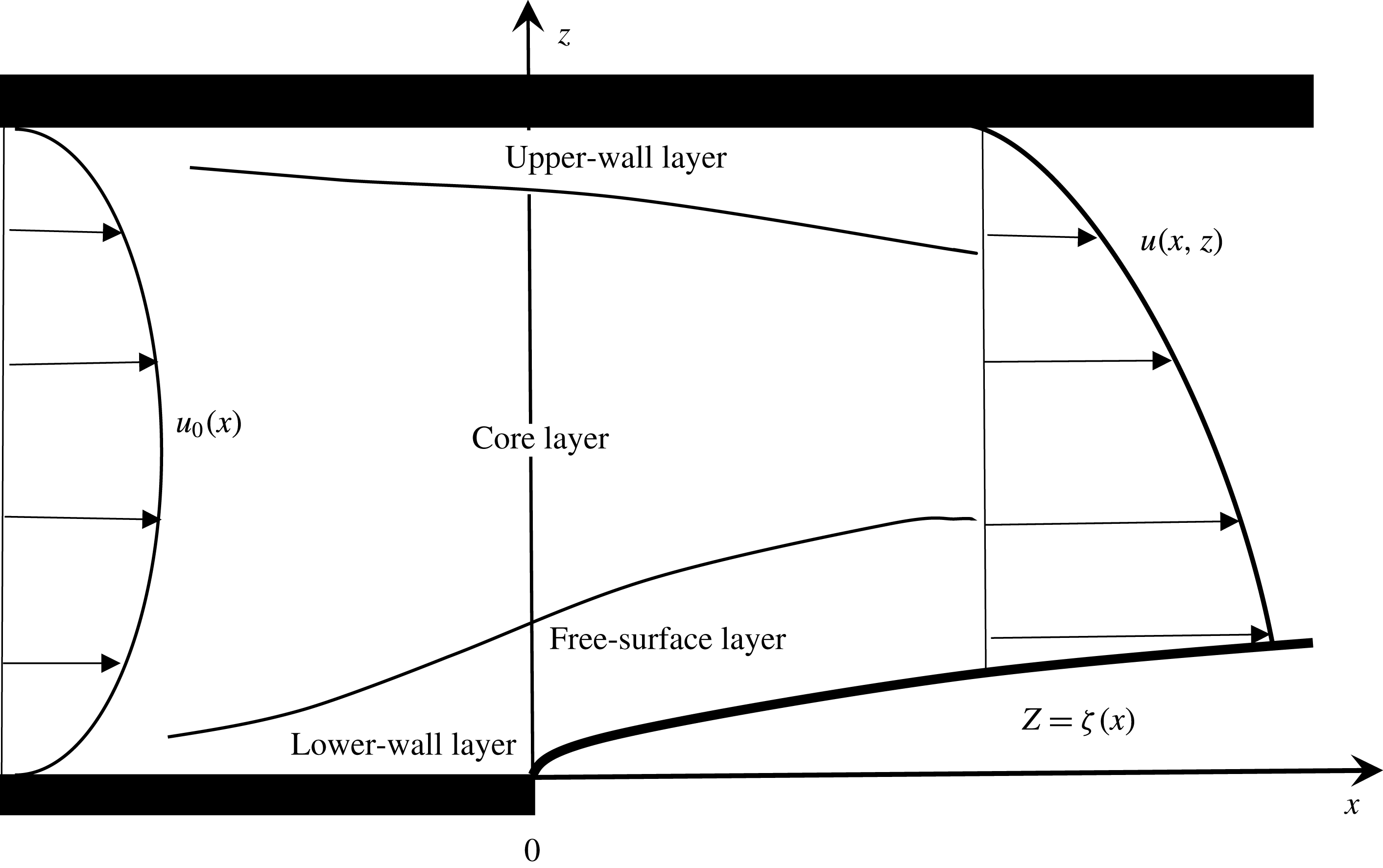
We examine the flow of a free-surface liquid jet as it emerges from a channel bounded by a semi-infinite lower wall and an infinite upper wall, as depicted in figure 1 below. We shall refer to this problem as free-surface wall-jet flow compared with the more common wall-jet flow when the jet emerges into the same ambient fluid. Inertia is assumed to remain relatively important, allowing asymptotic development of the flow field in terms of the inverse power of the Reynolds number. The jet is assumed to be subject to a constant pressure gradient far upstream where the flow acquires a Poiseuille character. Given its relevance to coating, free-surface wall-jet flow has been examined extensively, but mostly in the absence of inertia (Tanner Reference Tanner2000). Elliotis, Georgiou & Xenophontos (Reference Elliotis, Georgiou and Xenophontos2005) examined the creeping flow around the stress singularity as it passes from an adhering to a slippery straight wall. Of closer relevance to the current study is the treatment of Ruschak & Scriven (Reference Ruschak and Scriven1977), who examined the same flow configuration as in figure 1 below but for gravity-driven flow. They also used the method of matched asymptotic expansions, but limited their work to dominant surface tension and low inertia.
Schematic of the wall-jet problem (dimensionless notations are used). The boundary layers are depicted along the free surface, lower wall and upper wall.

When a free-surface viscous jet emerges from a tube or a channel, an abrupt change in stress occurs at the exit. This type of singularity constitutes the major difficulty in any theoretical analysis. If a computational approach is adopted, incorporation of the singularity point and its immediate vicinity is unavoidable since the entire flow domain must be considered (discretized). The singularity region, which is crucial to the rest of the flow domain, is difficult to handle numerically if a satisfactory level of accuracy is sought since typical numerical schemes tend to smooth out the singularity. In contrast, the asymptotic approach lends itself efficiently as a viable alternative since the singular point is avoided altogether because of the similar character of the flow near the free surface. Both analytical and computational solution methodologies have been pursued in the literature. A combination of analytical and numerical treatments has also been proposed (Shi, Breuer & Durst Reference Shi, Breuer and Durst2004). Higher accuracy is typically achieved through mesh refinement, which captures the singularity more effectively, but leads simultaneously to the presence of stronger flow gradients that are difficult to handle numerically (Pasquali & Scriven Reference Pasquali and Scriven2002).
Perhaps more importantly, asymptotics tend to provide a deeper insight into the flow structure near the singularity. The singularity is circumvented by identifying two distinct flow regions: a boundary-layer region near the free surface, extending towards but not including the singular point, and a core region where the flow remains close to fully developed. The inclusion of the singularity is not essential in this case given the similarity character of the flow in the boundary-layer region along the free surface. Asymptotic analysis has been successfully adopted for flows in the viscocapillary range (Goren & Wronski Reference Goren and Wronski1966; Ruschak & Scriven Reference Ruschak and Scriven1977; Higgins Reference Higgins1982; Benilov, Benilov & Kopteva Reference Benilov, Benilov and Kopteva2008), and, more closely to the present problem, in the viscoinertial range, but to a much lesser extent. Tillett (Reference Tillett1968) analysed the laminar symmetric free-jet flow near the channel exit using the method of matched asymptotic expansions. Miyake, Mukai & Iemoto (Reference Miyake, Mukai and Iemoto1979) carried out a similar analysis on a vertical jet of inviscid fluid, taking into account the gravity effect. Philippe & Dumargue (Reference Philippe and Dumargue1991) also applied a similar analysis to that of Tillett for viscous axisymmetric vertical jets, emphasizing the interplay between the effects of gravity and inertia on the free-surface shape and the velocity profile. A local similarity transformation was carried out by Wilson (Reference Wilson1986) for the axisymmetric viscous-gravity jet of the boundary-layer-type flow close to the free surface. Recently, Khayat (Reference Khayat2016a ,Reference Khayat b ) examined the flow of a jet emerging from a hydrophobic channel. Asymptotic analyses have also been successfully implemented for non-Newtonian jet flow; see, for instance, the work on the flow exiting a channel of a power-law fluid by Khayat (Reference Khayat2014) and a viscoelastic fluid by Saffari & Khayat (Reference Saffari and Khayat2009).
For a recent perspective on asymptotic analyses, their applications and historic development, the reader is referred to the book by Sobey (Reference Sobey2000) on interactive boundary-layer and triple-deck theory. In this regard, and despite the presence of three layers for the current problem, a triple-deck approach is not exactly applicable given the absence of an inviscid (external) layer. A closer treatment would be that of Smith (Reference Smith1979) on the flow in a tube with severe (axisymmetric) constriction. Smith realized that a similar model to the triple-deck formulation, based on an inviscid rotational core flow region together with viscous boundary-layer-type regions near the walls, could be applied to the flow in the vicinity of the constriction. Similarly, a classical boundary-layer analysis is developed in the present problem near the free surface and upper wall, and the boundary-layer flow is matched to the inviscid flow in the core region. The flow field is thus determined at small distances downstream of the jet. As in typical boundary-layer analyses, where the solution is not valid within a small distance from inception such as very near a leading edge or a stagnation point (for an impinging jet), the analysis precludes the flow at the channel exit. However, the distance in question is small, of the order of the (local) boundary-layer thickness. Consequently, the boundary-layer approach turns out to be successful in capturing the flow nature near inception. Special emphasis is placed on the effect of inertia on the shape of the free surface and the flow along the surface, as well as the profiles of the velocity and stress components near the upper and lower walls.
The problem is first examined in § 2, where the governing equations and boundary conditions are given. The overall flow structure is also discussed. The boundary-layer flows are sought in § 3 by considering separately the flow near the free surface, close to the lower wall and close to the upper wall. The flow in the core layer is covered in § 4. Part of the formulation in the free-surface and core layers is similar to the free-jet formulation carried out by Tillett (Reference Tillett1968) and Khayat and coworkers in the Newtonian limit (Saffari & Khayat Reference Saffari and Khayat2009; Khayat Reference Khayat2014). Consequently, the formulation of the flow near the walls will be emphasized.
2 Problem formulation and flow structure
Consider the laminar steady two-dimensional flow of an incompressible fluid of density
 $\unicode[STIX]{x1D70C}$
and viscosity
 $\unicode[STIX]{x1D707}$
, emerging from a channel of width
 $D$
, and continuously adhering to the upper infinite wall, as illustrated schematically in figure 1 in the (
 $x,z$
) plane. The
 $x$
-axis is taken along the lower wall and the
 $z$
-axis lies in the transverse direction across the channel. The channel exit coincides with
 $x=0$
. Far upstream, the flow is induced by a pressure gradient,
 $G$
, inside the channel. Non-dimensional variables are introduced by measuring lengths with respect to
 $D$
, streamfunction with respect to
 $VD$
and pressure with respect to
 $\unicode[STIX]{x1D70C}V^{2}$
, where
 $V=-(G/12\unicode[STIX]{x1D707})D^{2}$
is the mean velocity. In this case, the Reynolds number is given by
 $Re=DV/\unicode[STIX]{x1D708}$
, where
 $\unicode[STIX]{x1D708}$
is the kinematic viscosity. The Poiseuille streamfunction will turn out to be the leading-order solution in the core region, and is conveniently introduced here along with the velocity in dimensionless form as
 $$\begin{eqnarray}\displaystyle \unicode[STIX]{x1D713}_{0}(z)=3z^{2}-2z^{3},\quad u_{0}(z)=6z-6z^{2}. & & \displaystyle\end{eqnarray}$$
2.1 Governing equations and boundary conditions
The conservation of linear momentum equation takes the following dimensionless form:
 $$\begin{eqnarray}\displaystyle & \displaystyle \unicode[STIX]{x1D713}_{z}\unicode[STIX]{x1D713}_{xz}-\unicode[STIX]{x1D713}_{x}\unicode[STIX]{x1D713}_{zz}=-p_{x}+\frac{1}{Re}(\unicode[STIX]{x1D713}_{xxz}+\unicode[STIX]{x1D713}_{zzz}), & \displaystyle\end{eqnarray}$$
 $$\begin{eqnarray}\displaystyle & \displaystyle -\unicode[STIX]{x1D713}_{z}\unicode[STIX]{x1D713}_{xx}+\unicode[STIX]{x1D713}_{x}\unicode[STIX]{x1D713}_{xz}=-p_{z}-\frac{1}{Re}(\unicode[STIX]{x1D713}_{xxx}+\unicode[STIX]{x1D713}_{xzz}). & \displaystyle\end{eqnarray}$$
For
 $x>0$
, the kinematic and dynamic boundary conditions at the free surface
 $z=\unicode[STIX]{x1D701}(x)$
are
 $$\begin{eqnarray}\displaystyle & \displaystyle \unicode[STIX]{x1D713}(x>0,z=\unicode[STIX]{x1D701})=0, & \displaystyle\end{eqnarray}$$
 $$\begin{eqnarray}\displaystyle & \displaystyle p(x>0,z=\unicode[STIX]{x1D701})+\frac{1}{Re}[2\unicode[STIX]{x1D713}_{xz}+\unicode[STIX]{x1D701}^{\prime }(\unicode[STIX]{x1D713}_{zz}-\unicode[STIX]{x1D713}_{xx})]_{x>0,z=\unicode[STIX]{x1D701}}=0, & \displaystyle\end{eqnarray}$$
 $$\begin{eqnarray}\displaystyle & \displaystyle p(x>0,z=\unicode[STIX]{x1D701})\unicode[STIX]{x1D701}^{\prime }-\frac{1}{Re}(2\unicode[STIX]{x1D713}_{xz}\unicode[STIX]{x1D701}^{\prime }-\unicode[STIX]{x1D713}_{zz}+\unicode[STIX]{x1D713}_{xx})_{x>0,z=\unicode[STIX]{x1D701}}=0. & \displaystyle\end{eqnarray}$$
A prime denotes total differentiation with respect to the independent variable. In addition, the following conditions must be satisfied:
 $$\begin{eqnarray}\displaystyle & \displaystyle \unicode[STIX]{x1D713}_{z}(-\infty <x<\infty ,z=1)=\unicode[STIX]{x1D713}_{x}(-\infty <x<\infty ,z=1)=0, & \displaystyle\end{eqnarray}$$
 $$\begin{eqnarray}\displaystyle & \displaystyle \unicode[STIX]{x1D713}_{z}(x<0,z=0)=\unicode[STIX]{x1D713}_{x}(x<0,z=0)=0, & \displaystyle\end{eqnarray}$$
 $$\begin{eqnarray}\displaystyle & \displaystyle \unicode[STIX]{x1D713}(x\rightarrow -\infty ,z)\sim 3z^{2}-2z^{3}. & \displaystyle\end{eqnarray}$$
2.2 The flow structure and solution strategy
The flow is assumed to have the base Poiseuille profile (2.1) to lowest order, and is modified when the fluid leaves the channel in the form of the wall jet. When the fluid detaches itself from the lower wall of the channel, the removal of the wall stress causes a boundary layer to form in a region near the free surface. In this region, the parabolic velocity profile adjusts itself so as to satisfy the condition of zero traction at the free surface. In the inviscid limit of infinite Reynolds number, this condition would not be imposed since there is no (viscous) mechanism for the stress singularity to diffuse, and all of the conditions of the problem would be satisfied by observing that the Poiseuille profile continues undisturbed in the jet region. However, there is no unique solution for this inviscid problem, and we can assume that the fully developed Poiseuille flow is everywhere the proper inviscid limit. With this assumption, the flow in the core of the jet is, to lowest order, not affected by the flow in the boundary-layer region near the free surface although the boundary layer is expected to induce perturbations to the base Poiseuille flow when higher-order terms are included, for the flow both upstream and downstream of the channel exit. This assumption is similar to the one made for channel and tube flows with mild (Smith Reference Smith1976a ,Reference Smith b ) and severe (Smith Reference Smith1979) constrictions, where the flow field in the core region, to leading order, satisfies the inviscid equations of motion. Further discussion and comparison between the current and Smith’s formulations are given in § 4. The reader is also referred to Sobey (Reference Sobey2000) for other asymptotic analyses on interactive boundary layers.
When the fluid exits the channel, the vanishing of lower-wall shear stress at the channel exit causes a boundary layer to develop adjacent to the free surface, which we shall denote as the free-surface layer. This thin layer and the jet contraction (and expansion further downstream of the channel exit) affect the core of the jet, with this core layer remaining predominantly of inviscid rotational character. This inviscid layer cannot, however, extend to the wall, where significant viscous shearing occurs, forcing the formation of an upper-wall layer in the vicinity of the upper wall. Similarly, the core flow must also adjust to the shearing viscous flow in the lower-wall layer upstream of the stress singularity at the exit. In other words, given the predominantly inviscid character of the core flow, the core solution cannot satisfy adherence at the lower and upper walls. The thickness of the wall layers upstream of the channel exit is not expected to be significant at large Reynolds number, but can be large otherwise, and is fundamentally important to examine as it reflects the extent of upstream influence. In fact, the thickness of the wall layers will turn out to be of
 $O(Re^{-1})$
. The upper-wall layer downstream of the channel exit is expected to grow rapidly with distance.
Figure 1 illustrates schematically the different flow regions for the wall jet. In each layer, different physical mechanisms dominate the flow with corresponding characteristic length scales. In particular, for the flow downstream of the channel exit, the free-surface and upper-wall layers are shear dominated, and the flow is of the boundary-layer type. In the region in between, or the core layer, both shear and elongation are in balance as a result of the predominance of the Poiseuille character of the flow upstream and downstream of the channel exit. At the channel exit,
 $x=0$
, the shear stress undergoes a step change from a non-zero value at the lower wall,
 $z=0$
, to zero at the free surface,
 $z=\unicode[STIX]{x1D701}(x)$
. The effect of this drop diffuses upstream inside the channel
 $(x<0)$
, over a distance
 $x_{0}$
where fully developed Poiseuille flow is recovered, and downstream (
 $x>0$
), towards the upper wall. Boundary-layer solutions are sought near the free surface and walls, but not all layers admit a similarity solution. For the flow outside the channel, a similarity solution is sought in the free-surface layer, which is matched onto the core solution. The core flow, in turn, is matched onto the solution in the core region inside the channel at the exit, as well as onto the flow in the upper-wall layer. It is important to observe that no matching is required for the similarity flow at
 $x=0$
between the free-surface and lower-wall layers; the flow singularity at the origin is entirely avoided in the solution process. This constitutes a major advantage of the current formulation.
The present analysis is reminiscent of the ideas advanced in Stewartson’s triple-deck theory (Sobey Reference Sobey2000), which lays down a rational basis for the investigation of separation and other nonlinear features in external flow situations. The fundamental difference between the external separation phenomenon and the current wall-jet flow through a channel is the absence of an external inviscid region in the latter case. A similar approach was followed by Smith (Reference Smith1976a ,Reference Smith b , Reference Smith1979), who examined the fully developed flow through an indented tube when the Reynolds number is large. As in the current problem, there is no external flow region, and the triple-deck formulation could not simply be carried over to Smith’s problem, but, as mentioned earlier, Smith realized that a model based on an inviscid rotational core flow region together with viscous boundary-layer-type regions near the walls could be applied to his problem.
3 The flow near the free surface and near the walls
In this section, the flow structures in the boundary layer near the free surface, as well as near the upper and lower walls, are examined separately. In each layer, the near-boundary transverse coordinate will be denoted by
 $y=\unicode[STIX]{x1D700}\unicode[STIX]{x1D702}$
, where
 $\unicode[STIX]{x1D700}(Re)\ll 1$
is the small parameter in the problem, which will be precisely defined shortly. This notation will be the same in each layer, but takes different meanings. The usual conditions will be imposed, such as adherence and no-penetration conditions at the walls, and kinematic and dynamic conditions at the jet surface. Additional conditions are needed and are obtained by matching the flow at the outer edge of each boundary layer with the core flow, which is covered in § 4. Matching also provides conditions needed to obtain the core streamfunction and pressure terms
 $\unicode[STIX]{x1D713}_{m}(x,z)$
and
 $p_{m}(x,z)$
for
 $m\geqslant 0$
in expansions (4.1) and (4.2) respectively. The matching rule employed by Van Dyke (Reference Van Dyke1964) is adopted in each case, namely
 $$\begin{eqnarray}\displaystyle E_{n}H_{m}\unicode[STIX]{x1D713}=H_{m}E_{n}\unicode[STIX]{x1D713}, & & \displaystyle\end{eqnarray}$$
where
 $m$
and
 $n$
are integers. Here,
 $E_{n}$
is the core-expansion operator, which truncates immediately after the term of order
 $\unicode[STIX]{x1D700}^{n}$
, where the expansion is expressed in terms of core variables. The term
 $H_{m}$
is the corresponding boundary-layer expansion operator. We anticipate that the streamwise coordinate transformation
 $x(\unicode[STIX]{x1D709},\unicode[STIX]{x1D702})=\unicode[STIX]{x1D709}$
will be the same in all three cases treated, but the transformation
 $z(\unicode[STIX]{x1D709},\unicode[STIX]{x1D702})$
will be different. Consequently, although each boundary-layer flow must match the Poiseuille flow to leading order in the core layer, the governing equations for the streamfunction and pressure, as well as their perturbation expansions, will be different. Although
 $\unicode[STIX]{x1D709}=x$
, the use of
 $\unicode[STIX]{x1D709}$
instead of
 $x$
helps to emphasize the distinction between the core region where the (
 $x,z$
) variables are used and the boundary-layer region(s) where the
 $(\unicode[STIX]{x1D709},\unicode[STIX]{x1D702})$
variables are used, and makes clearer the mathematical development in each region.
3.1 The jet thickness and the flow in the free-surface layer
To examine the free-surface-layer structure, we let
 $y=z-\unicode[STIX]{x1D701}(x)$
. The scaling in the transverse direction is changed by writing
 $y=\unicode[STIX]{x1D700}\unicode[STIX]{x1D702}$
, where
 $\unicode[STIX]{x1D700}=Re^{-\unicode[STIX]{x1D6FC}}$
is the small parameter in the problem and
 $\unicode[STIX]{x1D6FC}$
is to be determined. Following Tillett (Reference Tillett1968), and anticipating that the height
 $\unicode[STIX]{x1D701}$
of the free surface is of the same order of magnitude as the boundary-layer thickness, one can write
 $\unicode[STIX]{x1D701}(x)=\unicode[STIX]{x1D700}h(x)$
, and henceforth work with
 $h(x)$
. The matching indicates that
 $h=O(1)$
. The following change of coordinates is introduced:
 $$\begin{eqnarray}\displaystyle x=\unicode[STIX]{x1D709},\quad z=y+\unicode[STIX]{x1D701}(x)=\unicode[STIX]{x1D700}(\unicode[STIX]{x1D702}+h). & & \displaystyle\end{eqnarray}$$
The aim is to find a solution of problem (2.2)–(2.4) in the form of a boundary-layer expansion in
 $\unicode[STIX]{x1D700}$
. In order to match this to the core flow, it is necessary to have
 $\unicode[STIX]{x1D713}\sim y^{2}$
as
 $\unicode[STIX]{x1D702}\rightarrow \infty$
in the free-surface layer, to lowest order in
 $\unicode[STIX]{x1D700}$
(see below). Therefore,
 $\unicode[STIX]{x1D713}$
must be of order
 $\unicode[STIX]{x1D700}^{2}$
. As in the case of a symmetric jet (Tillett Reference Tillett1968), the value of
 $\unicode[STIX]{x1D6FC}$
is determined by requiring that the convective and viscous terms balance, leading to
 $\unicode[STIX]{x1D6FC}=1/3$
. The streamwise and transverse velocity components are expressed as
 $u=\unicode[STIX]{x1D713}_{z}=(1/\unicode[STIX]{x1D700})\unicode[STIX]{x1D713}_{\unicode[STIX]{x1D702}}$
and
 $w=-\unicode[STIX]{x1D713}_{x}=-\unicode[STIX]{x1D713}_{\unicode[STIX]{x1D709}}+h^{\prime }\unicode[STIX]{x1D713}_{\unicode[STIX]{x1D702}}$
. Throughout the paper, a prime is used to denote total differentiation (not necessarily only with respect to
 $x$
or
 $\unicode[STIX]{x1D709}$
). Considering the fact that
 $u$
in the free-surface layer must match the velocity in the core layer,
 $u\sim 6(z-z^{2})$
, it is also inferred that
 $u$
must be of order
 $\unicode[STIX]{x1D700}$
. Consequently,
 $w$
is of order
 $\unicode[STIX]{x1D700}^{2}$
. The momentum conservation equations (2.2) are rewritten as
 $$\begin{eqnarray}\displaystyle & & \displaystyle \unicode[STIX]{x1D713}_{\unicode[STIX]{x1D702}}\unicode[STIX]{x1D713}_{\unicode[STIX]{x1D709}\unicode[STIX]{x1D702}}-\unicode[STIX]{x1D713}_{\unicode[STIX]{x1D709}}\unicode[STIX]{x1D713}_{\unicode[STIX]{x1D702}\unicode[STIX]{x1D702}}=-\unicode[STIX]{x1D700}^{2}(p_{\unicode[STIX]{x1D709}}-h^{\prime }p_{\unicode[STIX]{x1D702}})+\unicode[STIX]{x1D700}^{2}\unicode[STIX]{x1D713}_{\unicode[STIX]{x1D702}\unicode[STIX]{x1D702}\unicode[STIX]{x1D702}}\qquad \qquad \qquad \qquad \nonumber\\ \displaystyle & & \displaystyle \;\;\;\quad \qquad \qquad \qquad +\,\unicode[STIX]{x1D700}^{4}(\unicode[STIX]{x1D713}_{\unicode[STIX]{x1D709}\unicode[STIX]{x1D709}\unicode[STIX]{x1D702}}-h^{\prime \prime }\unicode[STIX]{x1D713}_{\unicode[STIX]{x1D702}\unicode[STIX]{x1D702}}-2h^{\prime }\unicode[STIX]{x1D713}_{\unicode[STIX]{x1D709}\unicode[STIX]{x1D702}\unicode[STIX]{x1D702}}+h^{\prime 2}\unicode[STIX]{x1D713}_{\unicode[STIX]{x1D702}\unicode[STIX]{x1D702}\unicode[STIX]{x1D702}}),\end{eqnarray}$$
 $$\begin{eqnarray}\displaystyle & & \displaystyle -\unicode[STIX]{x1D713}_{\unicode[STIX]{x1D702}}\unicode[STIX]{x1D713}_{\unicode[STIX]{x1D709}\unicode[STIX]{x1D709}}+\unicode[STIX]{x1D713}_{\unicode[STIX]{x1D709}}\unicode[STIX]{x1D713}_{\unicode[STIX]{x1D709}\unicode[STIX]{x1D702}}+h^{\prime \prime }\unicode[STIX]{x1D713}_{\unicode[STIX]{x1D702}}^{2}+h^{\prime }(\unicode[STIX]{x1D713}_{\unicode[STIX]{x1D702}}\unicode[STIX]{x1D713}_{\unicode[STIX]{x1D709}\unicode[STIX]{x1D702}}-\unicode[STIX]{x1D713}_{\unicode[STIX]{x1D709}}\unicode[STIX]{x1D713}_{\unicode[STIX]{x1D702}\unicode[STIX]{x1D702}})=-p_{\unicode[STIX]{x1D702}}-\unicode[STIX]{x1D700}^{2}(\unicode[STIX]{x1D713}_{\unicode[STIX]{x1D709}\unicode[STIX]{x1D702}\unicode[STIX]{x1D702}}-h^{\prime }\unicode[STIX]{x1D713}_{\unicode[STIX]{x1D702}\unicode[STIX]{x1D702}\unicode[STIX]{x1D702}})\qquad \nonumber\\ \displaystyle & & \displaystyle \;\;\;\quad \qquad \qquad \qquad -\,\unicode[STIX]{x1D700}^{4}\left(\frac{\unicode[STIX]{x2202}}{\unicode[STIX]{x2202}\unicode[STIX]{x1D709}}-h^{\prime }\frac{\unicode[STIX]{x2202}}{\unicode[STIX]{x2202}\unicode[STIX]{x1D702}}\right)^{3}\unicode[STIX]{x1D713}.\end{eqnarray}$$
The boundary conditions on the free surface
 $\unicode[STIX]{x1D702}=0$
are obtained from (2.3) to read
 $$\begin{eqnarray}\displaystyle & \displaystyle \unicode[STIX]{x1D713}=0, & \displaystyle\end{eqnarray}$$
 $$\begin{eqnarray}\displaystyle & \displaystyle h^{\prime }p+\unicode[STIX]{x1D713}_{\unicode[STIX]{x1D702}\unicode[STIX]{x1D702}}-\unicode[STIX]{x1D700}^{2}\left[\left(\frac{\unicode[STIX]{x2202}}{\unicode[STIX]{x2202}\unicode[STIX]{x1D709}}-h^{\prime }\frac{\unicode[STIX]{x2202}}{\unicode[STIX]{x2202}\unicode[STIX]{x1D702}}\right)^{2}\unicode[STIX]{x1D713}+2h^{\prime }(\unicode[STIX]{x1D713}_{\unicode[STIX]{x1D709}\unicode[STIX]{x1D702}}-h^{\prime }\unicode[STIX]{x1D713}_{\unicode[STIX]{x1D702}\unicode[STIX]{x1D702}})\right]=0, & \displaystyle\end{eqnarray}$$
 $$\begin{eqnarray}\displaystyle & \displaystyle p+\unicode[STIX]{x1D700}^{2}(2\unicode[STIX]{x1D713}_{\unicode[STIX]{x1D709}\unicode[STIX]{x1D702}}-h^{\prime }\unicode[STIX]{x1D713}_{\unicode[STIX]{x1D702}\unicode[STIX]{x1D702}})-\unicode[STIX]{x1D700}^{4}h^{\prime }\left(\frac{\unicode[STIX]{x2202}}{\unicode[STIX]{x2202}\unicode[STIX]{x1D709}}-h^{\prime }\frac{\unicode[STIX]{x2202}}{\unicode[STIX]{x2202}\unicode[STIX]{x1D702}}\right)^{2}\unicode[STIX]{x1D713}=0. & \displaystyle\end{eqnarray}$$
The expansion proceeds in powers of
 $\unicode[STIX]{x1D700}$
, so that
 $$\begin{eqnarray}\displaystyle \unicode[STIX]{x1D713}(\unicode[STIX]{x1D709},\unicode[STIX]{x1D702})=\unicode[STIX]{x1D700}^{2}\unicode[STIX]{x1D6F9}_{2}(\unicode[STIX]{x1D709},\unicode[STIX]{x1D702})+\unicode[STIX]{x1D700}^{3}\unicode[STIX]{x1D6F9}_{3}(\unicode[STIX]{x1D709},\unicode[STIX]{x1D702})+\cdots \,. & & \displaystyle\end{eqnarray}$$
Similarly,
 $h$
is expanded as
 $$\begin{eqnarray}\displaystyle h(\unicode[STIX]{x1D709})=\unicode[STIX]{x1D700}^{-1}\unicode[STIX]{x1D701}(\unicode[STIX]{x1D709})=h_{0}(\unicode[STIX]{x1D709})+\unicode[STIX]{x1D700}h_{1}(\unicode[STIX]{x1D709})+\cdots \,. & & \displaystyle\end{eqnarray}$$
From (3.3) to (3.6), it is concluded that
 $p$
is of order
 $\unicode[STIX]{x1D700}^{4}$
. Thus,
 $$\begin{eqnarray}\displaystyle p(\unicode[STIX]{x1D709},\unicode[STIX]{x1D702})=\unicode[STIX]{x1D700}^{4}P_{4}(\unicode[STIX]{x1D709},\unicode[STIX]{x1D702})+\unicode[STIX]{x1D700}^{5}P_{5}(\unicode[STIX]{x1D709},\unicode[STIX]{x1D702})+\cdots \,. & & \displaystyle\end{eqnarray}$$
It is important to distinguish (3.5) from expression (4.1) for the flow in the core layer. Recalling that, to leading order, the streamfunction in the core layer is
 $\unicode[STIX]{x1D713}_{0}=3z^{2}-2z^{3}$
, it is useful to rewrite (4.1) in terms of the core variable
 $y=z-\unicode[STIX]{x1D701}$
and
 $h$
as
 $$\begin{eqnarray}\displaystyle \unicode[STIX]{x1D713}(x,z)=3(y+\unicode[STIX]{x1D700}h)^{2}-2(y+\unicode[STIX]{x1D700}h)^{3}+\unicode[STIX]{x1D700}\unicode[STIX]{x1D713}_{1}(x,z=y+\unicode[STIX]{x1D700}h)+\cdots \,, & & \displaystyle\end{eqnarray}$$
which will be referred to shortly. Now, consider the leading-order solution of problem (3.3)–(3.4). The equations reduce to
 $$\begin{eqnarray}\displaystyle & \displaystyle \unicode[STIX]{x1D6F9}_{2\unicode[STIX]{x1D702}}\unicode[STIX]{x1D6F9}_{2\unicode[STIX]{x1D709}\unicode[STIX]{x1D702}}-\unicode[STIX]{x1D6F9}_{2\unicode[STIX]{x1D709}}\unicode[STIX]{x1D6F9}_{2\unicode[STIX]{x1D702}\unicode[STIX]{x1D702}}=\unicode[STIX]{x1D6F9}_{2\unicode[STIX]{x1D702}\unicode[STIX]{x1D702}\unicode[STIX]{x1D702}}, & \displaystyle\end{eqnarray}$$
 $$\begin{eqnarray}\displaystyle & \displaystyle -\unicode[STIX]{x1D6F9}_{2\unicode[STIX]{x1D702}}\unicode[STIX]{x1D6F9}_{2\unicode[STIX]{x1D709}\unicode[STIX]{x1D709}}+\unicode[STIX]{x1D6F9}_{2\unicode[STIX]{x1D709}}\unicode[STIX]{x1D6F9}_{2\unicode[STIX]{x1D709}\unicode[STIX]{x1D702}}+h^{\prime \prime }\unicode[STIX]{x1D6F9}_{2\unicode[STIX]{x1D702}}^{2}+h^{\prime }(\unicode[STIX]{x1D6F9}_{2\unicode[STIX]{x1D702}}\unicode[STIX]{x1D6F9}_{2\unicode[STIX]{x1D709}\unicode[STIX]{x1D702}}-\unicode[STIX]{x1D6F9}_{2\unicode[STIX]{x1D709}}\unicode[STIX]{x1D6F9}_{2\unicode[STIX]{x1D702}\unicode[STIX]{x1D702}})=-P_{4\unicode[STIX]{x1D702}}-(\unicode[STIX]{x1D6F9}_{2\unicode[STIX]{x1D709}\unicode[STIX]{x1D702}\unicode[STIX]{x1D702}}-h^{\prime }\unicode[STIX]{x1D6F9}_{2\unicode[STIX]{x1D702}\unicode[STIX]{x1D702}\unicode[STIX]{x1D702}}). & \displaystyle \nonumber\\ \displaystyle & & \displaystyle\end{eqnarray}$$
Equation (3.9b ) is not needed immediately because of the decoupling of the pressure and streamfunction to this order. Two corresponding boundary conditions are obtained from (3.4), namely
 $$\begin{eqnarray}\displaystyle \unicode[STIX]{x1D6F9}_{2}(\unicode[STIX]{x1D709},\unicode[STIX]{x1D702}=0)=\unicode[STIX]{x1D6F9}_{2\unicode[STIX]{x1D702}\unicode[STIX]{x1D702}}(\unicode[STIX]{x1D709},\unicode[STIX]{x1D702}=0)=0. & & \displaystyle\end{eqnarray}$$
To complete the problem for
 $\unicode[STIX]{x1D6F9}_{2}$
, another boundary condition is required, which we will now obtain by matching the boundary-layer flow near the free surface with the core-layer flow downstream of the channel exit (see further below). The resulting condition reads
 $$\begin{eqnarray}\unicode[STIX]{x1D6F9}_{2}(\unicode[STIX]{x1D709},\unicode[STIX]{x1D702}\rightarrow \infty )\sim 3\unicode[STIX]{x1D702}^{2}.\end{eqnarray}$$
The boundary-layer growth above the free surface can be estimated from (3.9a
) and (3.11), which indicates that
 $\unicode[STIX]{x1D702}\propto \unicode[STIX]{x1D709}/\unicode[STIX]{x1D6F9}_{2}\sim \unicode[STIX]{x1D709}/\unicode[STIX]{x1D702}^{2}$
. This leads to
 $y\propto (x/Re)^{1/3}$
for the thickness of the free-surface layer. As we shall see, the boundary-layer growth is different along the walls.
The asymptotic form (3.11) for
 $\unicode[STIX]{x1D6F9}_{2}$
is determined by considering the application of (3.1) for
 $m=2$
and
 $n=0$
. Applying
 $E_{0}$
on (3.8) gives
 $$\begin{eqnarray}E_{0}\unicode[STIX]{x1D713}=3y^{2}-2y^{3}.\end{eqnarray}$$
In terms of the inner variable,
 $\unicode[STIX]{x1D702}$
,
 $E_{0}\unicode[STIX]{x1D713}=3\unicode[STIX]{x1D700}^{2}\unicode[STIX]{x1D702}^{2}-2\unicode[STIX]{x1D700}^{3}\unicode[STIX]{x1D702}^{3}$
. Therefore,
 $$\begin{eqnarray}\displaystyle H_{2}E_{0}\unicode[STIX]{x1D713}=3\unicode[STIX]{x1D700}^{2}\unicode[STIX]{x1D702}^{2}=3y^{2}. & & \displaystyle\end{eqnarray}$$
To leading order, the expansion for the streamfunction in the free-surface layer is obtained from (3.5) as
 $\unicode[STIX]{x1D713}=\unicode[STIX]{x1D700}^{2}\unicode[STIX]{x1D6F9}_{2}$
. Thus,
 $E_{0}H_{2}\unicode[STIX]{x1D713}=\unicode[STIX]{x1D700}^{2}\unicode[STIX]{x1D6F9}_{2}$
, which, when matched with (3.13), leads to condition (3.10). A similarity solution is carried out for
 $\unicode[STIX]{x1D6F9}_{2}$
, which is written here as
 $\unicode[STIX]{x1D6F9}_{2}(\unicode[STIX]{x1D709},\unicode[STIX]{x1D702})=\unicode[STIX]{x1D709}^{2/3}f_{2}(\unicode[STIX]{x1D703})$
, where
 $\unicode[STIX]{x1D703}=\unicode[STIX]{x1D702}\unicode[STIX]{x1D709}^{-1/3}$
is the similarity variable. The problem for
 $f_{2}(\unicode[STIX]{x1D703})$
is given by
 $$\begin{eqnarray}\displaystyle & \displaystyle 3f_{2}^{\prime \prime \prime }+(2f_{2}\,f_{2}^{\prime \prime }-f_{2}^{\prime 2})=0, & \displaystyle\end{eqnarray}$$
 $$\begin{eqnarray}\displaystyle & \displaystyle f_{2}(0)=f_{2}^{\prime \prime }(0)=0, & \displaystyle\end{eqnarray}$$
 $$\begin{eqnarray}\displaystyle & \displaystyle f_{2}(\unicode[STIX]{x1D703}\rightarrow \infty )\sim 3(\unicode[STIX]{x1D703}+c_{1})^{2}, & \displaystyle\end{eqnarray}$$
 $c_{1}$
is a constant to be determined numerically. Problem (3.14) is solved as an initial-value problem using a fourth-order Runge–Kutta scheme (IMSL-DIVERK), coupled to a shooting technique. Equation (3.14a
) is integrated subject to conditions (3.14b
) and a guessed value
 $f_{2}^{\prime }(0)$
for the slope at the origin. The slope is adjusted until reasonable matching is achieved with the asymptotic form (3.14c
) at large
 $\unicode[STIX]{x1D703}$
, or, more precisely, until
 $f_{2}^{\prime \prime }\sim 6$
is reached. The value of
 $c_{1}$
is then determined upon matching the numerical solution and its asymptotic form, which turns out to be
 $c_{1}=0.490$
.
Next, we determine
 $h_{0}(x)$
in (3.6) and the boundary condition for
 $\unicode[STIX]{x1D713}_{1}(x,z)$
in (3.8) or (4.1) by considering the application of (3.1) for
 $m=2$
and
 $n=1$
. Applying
 $E_{1}$
on (3.8), we have
 $$\begin{eqnarray}\displaystyle E_{1}\unicode[STIX]{x1D713}=3y^{2}-2y^{3}+\unicode[STIX]{x1D700}\unicode[STIX]{x1D713}_{1}(x,y). & & \displaystyle\end{eqnarray}$$
The terms surviving to
 $O(\unicode[STIX]{x1D700}^{2})$
are identified by expressing
 $E_{1}\unicode[STIX]{x1D713}$
in terms of
 $\unicode[STIX]{x1D702}=y/\unicode[STIX]{x1D700}$
, to yield
 $$\begin{eqnarray}\displaystyle H_{2}E_{1}\unicode[STIX]{x1D713}=3y^{2}+6\unicode[STIX]{x1D700}h_{0}y+\unicode[STIX]{x1D700}\unicode[STIX]{x1D713}_{1}(x,0)+\unicode[STIX]{x1D700}y\unicode[STIX]{x1D713}_{1y}(x,0)+\unicode[STIX]{x1D700}^{2}h_{0}\unicode[STIX]{x1D713}_{1y}(x,0). & & \displaystyle\end{eqnarray}$$
On the other hand, we note from (3.14c
) that
 $H_{2}\unicode[STIX]{x1D713}$
may be written in terms of the core variables as
 $$\begin{eqnarray}\displaystyle H_{2}\unicode[STIX]{x1D713}=\unicode[STIX]{x1D700}^{2}\unicode[STIX]{x1D709}^{2/3}f_{2}\sim 3\unicode[STIX]{x1D700}^{2}\unicode[STIX]{x1D709}^{2/3}(\unicode[STIX]{x1D703}+c_{1})^{2}=3\unicode[STIX]{x1D700}^{2}\unicode[STIX]{x1D709}^{2/3}(\unicode[STIX]{x1D702}\unicode[STIX]{x1D709}^{-1/3}+c_{1})^{2}=3(y+\unicode[STIX]{x1D700}c_{1}x^{1/3})^{2}. & & \displaystyle\end{eqnarray}$$
This yields
 $$\begin{eqnarray}\displaystyle E_{1}H_{2}\unicode[STIX]{x1D713}=3(y^{2}+2y\unicode[STIX]{x1D700}c_{1}x^{1/3}). & & \displaystyle\end{eqnarray}$$
Equating (3.16) and (3.18) leads to
 $$\begin{eqnarray}\displaystyle h_{0}(x)=c_{1}x^{1/3},\quad \unicode[STIX]{x1D713}_{1}(x>0,z=0)=0. & & \displaystyle\end{eqnarray}$$
The homogeneous boundary condition in (3.19) will be used in § 4 to determine the first-order term
 $\unicode[STIX]{x1D713}_{1}(x,z)$
in (4.1). It will turn out that
 $\unicode[STIX]{x1D713}_{1}(x,z)$
vanishes everywhere, which means that, to the order
 $\unicode[STIX]{x1D700}$
, there is no interaction between the boundary layer and the core flow.
The next step is to determine
 $\unicode[STIX]{x1D713}_{2}(x,z\rightarrow 0)$
in (3.8) or (4.1) by considering
 $m=n=2$
. Proceeding as before, we obtain
 $$\begin{eqnarray}\displaystyle & \displaystyle H_{2}E_{2}\unicode[STIX]{x1D713}=3y^{2}+6\unicode[STIX]{x1D700}h_{0}y+3\unicode[STIX]{x1D700}^{2}h_{0}^{2}+\unicode[STIX]{x1D700}^{2}\unicode[STIX]{x1D713}_{2}(x,0), & \displaystyle\end{eqnarray}$$
 $$\begin{eqnarray}\displaystyle & \displaystyle E_{2}H_{2}\unicode[STIX]{x1D713}=3(y^{2}+2y\unicode[STIX]{x1D700}c_{1}\unicode[STIX]{x1D709}^{1/3}+\unicode[STIX]{x1D700}^{2}\unicode[STIX]{x1D709}^{2/3}c_{1}^{2}). & \displaystyle\end{eqnarray}$$
Comparison yields
 $\unicode[STIX]{x1D713}_{2}(x,z\rightarrow 0)\sim 0$
. In this case,
 $\unicode[STIX]{x1D713}_{2}(x,z)$
also turns out to vanish everywhere. Consequently, the perturbation to the Poiseuille flow in the core layer is eventually reflected in the non-vanishing value of
 $\unicode[STIX]{x1D713}_{3}(x,z)$
in (3.8) or (4.1), which will be determined in § 4. Pursuing the matching process to next order to determine
 $\unicode[STIX]{x1D6F9}_{3}(\unicode[STIX]{x1D709},\unicode[STIX]{x1D702})$
, we have
 $$\begin{eqnarray}\displaystyle H_{3}E_{0}\unicode[STIX]{x1D713}=3\unicode[STIX]{x1D700}^{2}\unicode[STIX]{x1D702}^{2}-2\unicode[STIX]{x1D700}^{3}\unicode[STIX]{x1D702}^{3}. & & \displaystyle\end{eqnarray}$$
Noting that
 $E_{0}H_{3}\unicode[STIX]{x1D713}=\unicode[STIX]{x1D700}^{2}\unicode[STIX]{x1D6F9}_{2}+\unicode[STIX]{x1D700}^{3}\unicode[STIX]{x1D6F9}_{3}$
, and equating it to (3.22), leads to
 $\unicode[STIX]{x1D6F9}_{3}\sim -2\unicode[STIX]{x1D702}^{3}$
and confirms
 $\unicode[STIX]{x1D6F9}_{2}\sim 3\unicode[STIX]{x1D702}^{2}$
for large
 $\unicode[STIX]{x1D702}$
. A similarity solution is also possible for
 $\unicode[STIX]{x1D6F9}_{3}$
, which is written here as
 $\unicode[STIX]{x1D6F9}_{3}(\unicode[STIX]{x1D709},\unicode[STIX]{x1D702})=\unicode[STIX]{x1D709}f_{3}(\unicode[STIX]{x1D703})$
. The problem for
 $f_{3}(\unicode[STIX]{x1D703})$
becomes
 $$\begin{eqnarray}\displaystyle 3f_{3}^{\prime \prime \prime }+2f_{2}\,f_{3}^{\prime \prime }-3f_{2}^{\prime }\,f_{3}^{\prime }+3f_{2}^{\prime \prime }\,f_{3}=0, & & \displaystyle\end{eqnarray}$$
 $$\begin{eqnarray}\displaystyle f_{3}(0)=f_{3}^{\prime \prime }(0)=0,\quad f_{3}(\unicode[STIX]{x1D703}\rightarrow \infty )\sim -2[(\unicode[STIX]{x1D703}+c_{1})^{3}-1]+c_{2}(\unicode[STIX]{x1D703}+c_{1}). & & \displaystyle\end{eqnarray}$$
Here,
 $c_{2}=-2.931$
, which is determined numerically. The velocity to third order becomes
 $$\begin{eqnarray}\displaystyle u(\unicode[STIX]{x1D709},\unicode[STIX]{x1D703})=\unicode[STIX]{x1D700}\unicode[STIX]{x1D709}^{1/3}f_{2}^{\prime }(\unicode[STIX]{x1D703})+\unicode[STIX]{x1D700}^{2}\unicode[STIX]{x1D709}^{2/3}f_{3}^{\prime }(\unicode[STIX]{x1D703})+O(\unicode[STIX]{x1D700}^{3}). & & \displaystyle\end{eqnarray}$$
Although linear, problem (3.23) is of the two-point boundary-value type; it is solved numerically following the same scheme as for problem (3.14). As in typical boundary-layer similarity problems, convergence is achieved over a relatively short range for
 $\unicode[STIX]{x1D703}$
values. The interval
 $[0,10]$
was adequate for both problems. Of particular interest are the values of the slopes at the origin,
 $f_{2}^{\prime }(0)$
and
 $f_{3}^{\prime }(0)$
, which are directly related to the velocity at the free surface. In this case,
 $f_{2}^{\prime }(0)=5.319$
and
 $f_{3}^{\prime }(0)=-5.174$
.
The jet thickness to next order is now determined by setting
 $m=n=3$
in (3.1). Ensuring
 $E_{3}H_{3}\unicode[STIX]{x1D713}=H_{3}E_{3}\unicode[STIX]{x1D713}$
leads to
 $h_{1}=(c_{2}/6)x^{2/3}$
. Additionally, we have the following non-homogeneous condition for the core flow:
 $$\begin{eqnarray}\displaystyle \unicode[STIX]{x1D713}_{3}(x>0,z=0)=2x, & & \displaystyle\end{eqnarray}$$
which provides the third boundary condition,
 $w_{3}(x,0)=-\unicode[STIX]{x1D713}_{3x}(x,0)=-2$
, needed for the solution of
 $\unicode[STIX]{x1D713}_{3}(x,z)$
in the core layer (see § 4.1). The height of the free surface is then given by
 $$\begin{eqnarray}\displaystyle \unicode[STIX]{x1D701}(x)=\unicode[STIX]{x1D700}c_{1}x^{1/3}+\unicode[STIX]{x1D700}^{2}\frac{c_{2}}{6}x^{2/3}+O(\unicode[STIX]{x1D700}^{3}). & & \displaystyle\end{eqnarray}$$
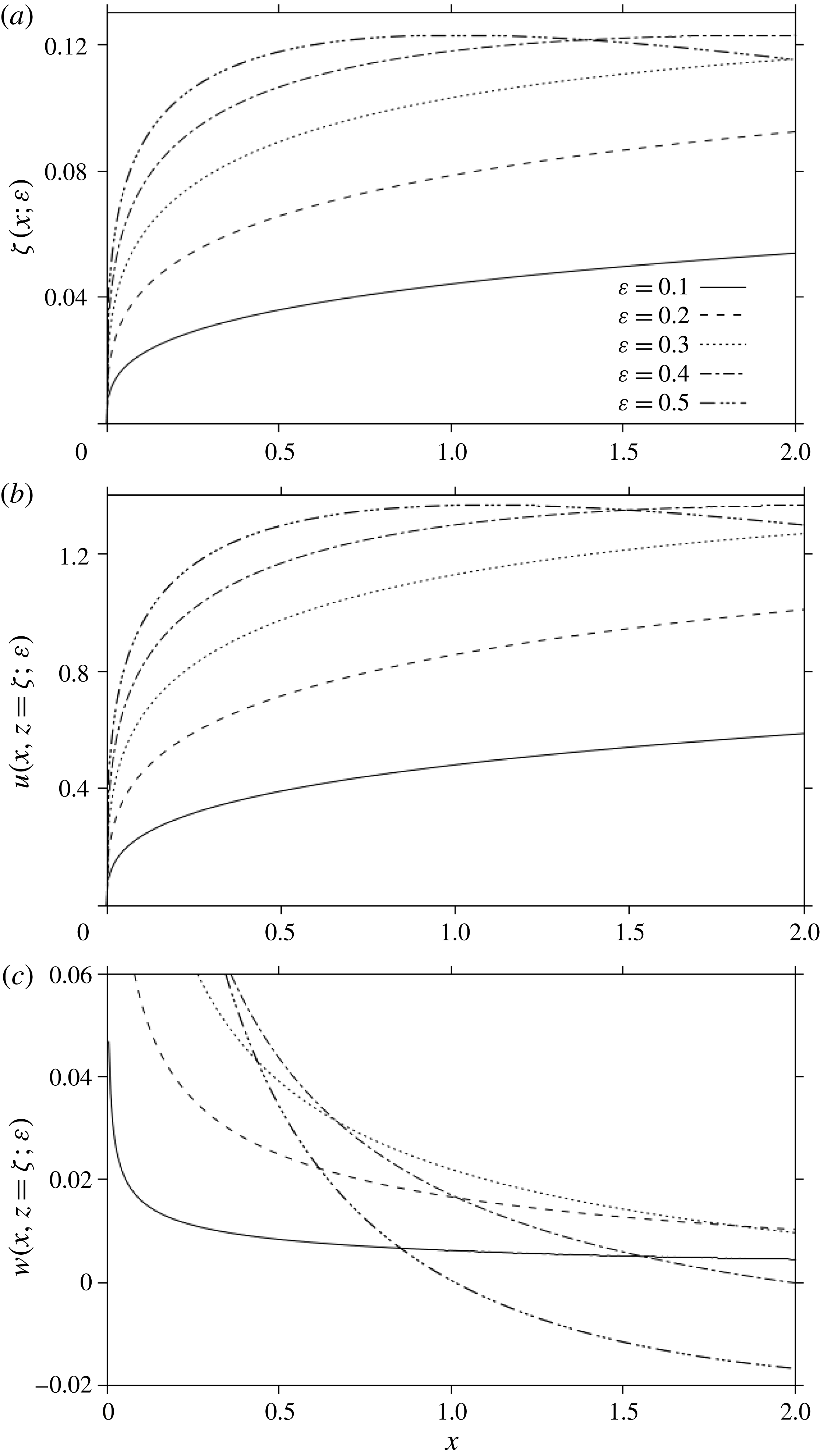
Figure 2 illustrates the influence of inertia on the jet thickness (figure 2
a), the streamwise (figure 2
b) and the transverse (figure 2
c) velocity components when plotted against distance from the channel exit. The profiles in figure 2(a) suggest that the jet always contracts near the exit. Although the jet is expected to eventually expand as a result of increasing friction along the upper wall, the maximum contraction and ensuing expansion, typically illustrated for
 $\unicode[STIX]{x1D700}=0.5$
, may not be accurately reflected here as
 $x$
must be
 $O(\unicode[STIX]{x1D700}^{-3})$
for (3.25) to remain uniformly valid. Moreover, the current formulation does not account for any interaction between the free-surface and wall layers (see § 3.3.2 for further discussion). The location of the maximum turns out to be simply proportional to the Reynolds number, namely
 $x_{m}=-(3c_{1}/\unicode[STIX]{x1D700}c_{2})^{3}=0.126Re$
. Interestingly, the actual value of the maximum surface height,
 $\unicode[STIX]{x1D701}_{m}=\unicode[STIX]{x1D701}(x=x_{m})$
, is independent of the Reynolds number, and is given by
 $\unicode[STIX]{x1D701}_{m}=-3c_{1}^{2}/2c_{2}=0.123$
. In contrast, the ensuing expansion depends strongly on inertia. Figure 2(b) displays the
 $u(x,z=\unicode[STIX]{x1D701})$
profiles, indicating velocity growth and decay with
 $x$
for the contracting and expanding jet portions respectively. As the jet expands, it behaves like typical wall jets, with the velocity decreasing linearly with distance (see figure 4 in Bakke (Reference Bakke1957)). The apparent decrease of the surface velocity with increasing inertia depicted in figure 2(b) is due to the scaling used. More important is the rapid increase in elongation rate near the exit,
 $u_{x}(x=0,z=0)$
, as inertia decreases. Elongation is also reflected in the jump in transverse flow (see figure 2
c). Given that the shearing near the exit does not change significantly, the relatively dominant elongation rate elsewhere causes the pressure to adjust suddenly (above the surface), suggesting the potential formation of an adverse pressure gradient resulting from the balance in streamwise linear momentum, which, in turn, may be conducive to flow separation at the upper wall. Flow reversal and separation in the current problem are the result of jet rapid contraction and expansion. The potential for separation will be discussed further when the pressure and shear stress are examined along the upper wall.
The influence of inertia on the jet thickness (a), streamwise (b) and transverse (c) velocity components, plotted against distance downstream of the channel exit.

Finally, the current treatment precludes a distance downstream very close to the channel exit (origin) where the stress singularity is located. In the free-surface layer, the situation is similar to classical boundary-layer flow, where the similarity solution is not valid near the singularity (leading edge). Incidentally, it is important to observe that, in addition to the stress singularity, the jet also experiences a geometrical singularity as the slope of the jet surface is discontinuous at
 $x=0$
. The free-surface height becomes itself discontinuous when higher-order terms are sought (Tillett Reference Tillett1968).
3.2 The flow in the lower-wall layer upstream of the exit (
 $x<0$
)

To examine the boundary-layer structure near the lower wall upstream of the channel exit, we introduce the near-wall coordinates as
 $x=\unicode[STIX]{x1D709}$
and
 $y=z=\unicode[STIX]{x1D700}\unicode[STIX]{x1D702}$
. As in the case near the free surface, matching with the core flow inside the channel shows that
 $\unicode[STIX]{x1D713}\sim 3y^{2}=3\unicode[STIX]{x1D700}^{2}\unicode[STIX]{x1D702}^{2}$
as
 $\unicode[STIX]{x1D702}\rightarrow \infty$
. Thus, we must have
 $\unicode[STIX]{x1D713}=O(\unicode[STIX]{x1D700}^{2})$
near the lower wall. In this case, the momentum conservation equations, along with the wall and upstream conditions, are
 $$\begin{eqnarray}\displaystyle & \displaystyle \unicode[STIX]{x1D713}_{\unicode[STIX]{x1D702}}\unicode[STIX]{x1D713}_{\unicode[STIX]{x1D709}\unicode[STIX]{x1D702}}-\unicode[STIX]{x1D713}_{\unicode[STIX]{x1D709}}\unicode[STIX]{x1D713}_{\unicode[STIX]{x1D702}\unicode[STIX]{x1D702}}=-\unicode[STIX]{x1D700}^{2}p_{\unicode[STIX]{x1D709}}+\unicode[STIX]{x1D700}^{2}\unicode[STIX]{x1D713}_{\unicode[STIX]{x1D702}\unicode[STIX]{x1D702}\unicode[STIX]{x1D702}}+\unicode[STIX]{x1D700}^{4}\unicode[STIX]{x1D713}_{\unicode[STIX]{x1D709}\unicode[STIX]{x1D709}\unicode[STIX]{x1D702}}, & \displaystyle\end{eqnarray}$$
 $$\begin{eqnarray}\displaystyle & \displaystyle \unicode[STIX]{x1D713}_{\unicode[STIX]{x1D702}}\unicode[STIX]{x1D713}_{\unicode[STIX]{x1D709}\unicode[STIX]{x1D709}}-\unicode[STIX]{x1D713}_{\unicode[STIX]{x1D709}}\unicode[STIX]{x1D713}_{\unicode[STIX]{x1D709}\unicode[STIX]{x1D702}}=p_{\unicode[STIX]{x1D702}}+\unicode[STIX]{x1D700}^{2}\unicode[STIX]{x1D713}_{\unicode[STIX]{x1D709}\unicode[STIX]{x1D702}\unicode[STIX]{x1D702}}+\unicode[STIX]{x1D700}^{4}\unicode[STIX]{x1D713}_{\unicode[STIX]{x1D709}\unicode[STIX]{x1D709}\unicode[STIX]{x1D709}}, & \displaystyle\end{eqnarray}$$
 $$\begin{eqnarray}\displaystyle \unicode[STIX]{x1D713}(\unicode[STIX]{x1D709},\unicode[STIX]{x1D702}=0)=\unicode[STIX]{x1D713}_{\unicode[STIX]{x1D702}}(\unicode[STIX]{x1D709},\unicode[STIX]{x1D702}=0)=0,\quad \unicode[STIX]{x1D713}(\unicode[STIX]{x1D709}\rightarrow -\infty ,\unicode[STIX]{x1D702})\sim 3\unicode[STIX]{x1D700}^{2}\unicode[STIX]{x1D702}^{2}-2\unicode[STIX]{x1D700}^{3}\unicode[STIX]{x1D702}^{3}. & & \displaystyle\end{eqnarray}$$
The velocity components become
 $u=(1/\unicode[STIX]{x1D700})\unicode[STIX]{x1D713}_{\unicode[STIX]{x1D702}}$
and
 $w=-\unicode[STIX]{x1D713}_{\unicode[STIX]{x1D709}}$
. Noting that
 $p$
is of order
 $\unicode[STIX]{x1D700}^{2}$
, the flow field expansion reads
 $$\begin{eqnarray}\displaystyle & \displaystyle \unicode[STIX]{x1D713}(\unicode[STIX]{x1D709},\unicode[STIX]{x1D702})=\unicode[STIX]{x1D700}^{2}\unicode[STIX]{x1D6F9}_{2}(\unicode[STIX]{x1D709},\unicode[STIX]{x1D702})+\unicode[STIX]{x1D700}^{3}\unicode[STIX]{x1D6F9}_{3}(\unicode[STIX]{x1D709},\unicode[STIX]{x1D702})+\cdots \,, & \displaystyle\end{eqnarray}$$
 $$\begin{eqnarray}\displaystyle & \displaystyle p(\unicode[STIX]{x1D709},\unicode[STIX]{x1D702})=\unicode[STIX]{x1D700}^{2}P_{2}(\unicode[STIX]{x1D709},\unicode[STIX]{x1D702})+\unicode[STIX]{x1D700}^{3}P_{3}(\unicode[STIX]{x1D709},\unicode[STIX]{x1D702})+\cdots \,. & \displaystyle\end{eqnarray}$$
Upon inserting (3.28) and (3.29) into (3.27), a hierarchy of problems is obtained to various orders. Each problem is of the boundary-layer type, requiring only one boundary condition in the streamwise direction. Consequently, the far-upstream condition in (3.27c,d
) is sufficient for well-posedness. This confirms that no matching is required with the free-surface-layer flow at the channel exit (
 $x=0$
). In this regard, a streamwise rescaling (of
 $x$
) is not necessary unless we wish to capture the flow structure very close to the origin. Consequently,
 $x$
is supposed to remain at least of
 $O(1)$
; the current treatment precludes a distance upstream very close to the origin. This is not the case for the flow in a constricted (dilated) channel, for instance, where
 $x$
is rescaled in terms of the inverse power of the indentation slope (and the Reynolds number), allowing the rapidly adjusting flow to be captured close to the inception of the constriction (dilation). In that case, the rescaling is necessary in order to determine the flow through and past the constriction (dilation) (Smith Reference Smith1976a
,Reference Smith
b
). In contrast, the current flow is not continuous through the singularity. Of closer relevance to the flow in the lower-wall layer is the flow near the trailing edge of a flat plate, where
 $x$
needs to be rescaled only if the flow very close to the singularity is to be determined; that is, when the distance is of the same order as the boundary-layer thickness. Although an analysis similar to that of the flow near the trailing edge could be envisaged, such an extensive analysis is not necessary here. In the lower-wall layer very near the origin, as near the trailing edge, the boundary-layer assumption breaks down as both elongation and shearing become equally dominant, and the full Navier–Stokes equations must be solved (see § 3 of Talke & Berger (Reference Talke and Berger1970)). Since the boundary-layer thickness turned out to be of order
 $1/Re$
, our results must be assumed to be invalid when
 $O(Re^{-1})<x<0$
.
We now consider the matching between the lower-wall and the core layers in order to derive the additional boundary conditions needed to solve problem (3.27). We recall first that in the core layer, the perturbations
 $\unicode[STIX]{x1D713}_{1}(x,z)=\unicode[STIX]{x1D713}_{2}(x,z)=0$
, so that (4.1) is conveniently reproduced here as
 $$\begin{eqnarray}\displaystyle \unicode[STIX]{x1D713}(x,z)=3y^{2}-2y^{3}+\unicode[STIX]{x1D700}^{3}\unicode[STIX]{x1D713}_{3}(x,z=y)+\cdots \,. & & \displaystyle\end{eqnarray}$$
Clearly,
 $E_{0}\unicode[STIX]{x1D713}=3y^{2}-2y^{3}$
, so that
 $H_{3}E_{0}\unicode[STIX]{x1D713}=3\unicode[STIX]{x1D700}^{2}\unicode[STIX]{x1D702}^{2}-2\unicode[STIX]{x1D700}^{3}\unicode[STIX]{x1D702}^{3}=3y^{2}-2y^{3}$
. Moreover, from (3.28), we have
 $H_{3}\unicode[STIX]{x1D713}=\unicode[STIX]{x1D700}^{2}\unicode[STIX]{x1D6F9}_{2}+\unicode[STIX]{x1D700}^{3}\unicode[STIX]{x1D6F9}_{3}$
. Setting
 $H_{3}E_{0}\unicode[STIX]{x1D713}=E_{0}H_{3}\unicode[STIX]{x1D713}$
, we deduce that
 $\unicode[STIX]{x1D6F9}_{2}\sim 3\unicode[STIX]{x1D702}^{2}$
and
 $\unicode[STIX]{x1D6F9}_{3}\sim -2\unicode[STIX]{x1D702}^{3}$
for large
 $\unicode[STIX]{x1D702}$
. In this case, it is not difficult to show that the solutions to
 $O(\unicode[STIX]{x1D700}^{2})$
and
 $O(\unicode[STIX]{x1D700}^{3})$
, which satisfy the homogeneous conditions at the wall and far-upstream condition in (3.27c,d
), are
 $$\begin{eqnarray}\displaystyle \unicode[STIX]{x1D6F9}_{2}(\unicode[STIX]{x1D709},\unicode[STIX]{x1D702})=3\unicode[STIX]{x1D702}^{2},\quad P_{2}(\unicode[STIX]{x1D709},\unicode[STIX]{x1D702})=0, & & \displaystyle\end{eqnarray}$$
 $$\begin{eqnarray}\displaystyle \unicode[STIX]{x1D6F9}_{3}(\unicode[STIX]{x1D709},\unicode[STIX]{x1D702})=-2\unicode[STIX]{x1D702}^{3},\quad P_{3}(\unicode[STIX]{x1D709},\unicode[STIX]{x1D702})=-12\unicode[STIX]{x1D709}. & & \displaystyle\end{eqnarray}$$
Thus, to
 $O(\unicode[STIX]{x1D700}^{3})$
, the flow retains its Poiseuille character near the lower wall.
Before proceeding to the next order, we need to determine the inner value
 $\unicode[STIX]{x1D713}_{3}(x<0,z\rightarrow 0)$
for the core flow problem. To this end, we note first from (3.30) that
 $$\begin{eqnarray}\displaystyle E_{3}\unicode[STIX]{x1D713}=3y^{2}-2y^{3}+\unicode[STIX]{x1D700}^{3}[\unicode[STIX]{x1D713}_{3}(x,0)+y\unicode[STIX]{x1D713}_{3y}(x,0)+{\textstyle \frac{1}{2}}y^{2}\unicode[STIX]{x1D713}_{3yy}(x,0)+\cdots \,], & & \displaystyle\end{eqnarray}$$
and, from (3.31) and (3.32), that
 $$\begin{eqnarray}\displaystyle H_{3}\unicode[STIX]{x1D713}=3\unicode[STIX]{x1D700}^{2}\unicode[STIX]{x1D702}^{2}-2\unicode[STIX]{x1D700}^{3}\unicode[STIX]{x1D702}^{3}. & & \displaystyle\end{eqnarray}$$
This leads to
 $H_{3}E_{3}\unicode[STIX]{x1D713}=3y^{2}-2y^{3}+\unicode[STIX]{x1D700}^{3}\unicode[STIX]{x1D713}_{3}(x,0)$
and
 $E_{3}H_{3}\unicode[STIX]{x1D713}=3y^{2}-2y^{3}$
, yielding
 $$\begin{eqnarray}\displaystyle \unicode[STIX]{x1D713}_{3}(x<0,z=0)=0, & & \displaystyle\end{eqnarray}$$
which is the condition needed to determine the core flow upstream of the channel exit (refer to problem (4.5) in the next section).
We turn next to finding the matching condition needed, in addition to the wall conditions, to determine the disturbances
 $\unicode[STIX]{x1D6F9}_{4}$
and
 $P_{4}$
, which reflect the deviation from Poiseuille flow. The equations for
 $\unicode[STIX]{x1D6F9}_{4}$
and
 $P_{4}$
are
 $$\begin{eqnarray}\displaystyle \unicode[STIX]{x1D6F9}_{2\unicode[STIX]{x1D702}}\unicode[STIX]{x1D6F9}_{4\unicode[STIX]{x1D709}\unicode[STIX]{x1D702}}-\unicode[STIX]{x1D6F9}_{4\unicode[STIX]{x1D709}}\unicode[STIX]{x1D6F9}_{2\unicode[STIX]{x1D702}\unicode[STIX]{x1D702}}=-P_{4\unicode[STIX]{x1D709}}+\unicode[STIX]{x1D6F9}_{4\unicode[STIX]{x1D702}\unicode[STIX]{x1D702}\unicode[STIX]{x1D702}},\quad P_{4\unicode[STIX]{x1D702}}=0. & & \displaystyle\end{eqnarray}$$
In this case,
 $P_{4}(\unicode[STIX]{x1D709},\unicode[STIX]{x1D702})\equiv P_{4}(\unicode[STIX]{x1D709})$
. Clearly, (3.36) confirms that the problem is of the boundary-layer type, requiring only one boundary condition in the streamwise direction. Taking
 $m=4$
and
 $n=3$
in (3.1), and comparing
 $H_{4}E_{3}\unicode[STIX]{x1D713}=3y^{2}-2y^{3}+\unicode[STIX]{x1D700}^{3}y\unicode[STIX]{x1D713}_{3y}(x,z=0)=3\unicode[STIX]{x1D700}^{2}\unicode[STIX]{x1D702}^{2}-2\unicode[STIX]{x1D700}^{3}\unicode[STIX]{x1D702}^{3}+\unicode[STIX]{x1D700}^{4}\unicode[STIX]{x1D702}\unicode[STIX]{x1D713}_{3z}(x,z=0)$
with
 $E_{3}H_{4}\unicode[STIX]{x1D713}=3\unicode[STIX]{x1D700}^{2}\unicode[STIX]{x1D702}^{2}-2\unicode[STIX]{x1D700}^{3}\unicode[STIX]{x1D702}^{3}+\unicode[STIX]{x1D700}^{4}\unicode[STIX]{x1D6F9}_{4}$
yields the desired matching condition, namely
 $\unicode[STIX]{x1D6F9}_{4}\sim \unicode[STIX]{x1D702}\unicode[STIX]{x1D713}_{3z}(x,z=0)$
for large
 $\unicode[STIX]{x1D702}$
, where
 $\unicode[STIX]{x1D713}_{3z}(\unicode[STIX]{x1D709},z=0)=\sum _{n=1}^{\infty }(A_{n}/\unicode[STIX]{x1D6FD}_{n})\text{e}^{\unicode[STIX]{x1D6FD}_{n}\unicode[STIX]{x1D709}}$
is deduced from (4.9) or (4.10). We note that
 $V_{n}^{\prime }(z=0)=1$
from the solution of the eigenvalue problem (4.8), with
 $\unicode[STIX]{x1D6FD}_{n}$
being the eigenvalues. We also note that the coefficients
 $A_{n}$
are obtained from matching the flow at
 $x=0$
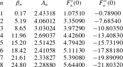
in the core layer as per (4.18). The values for the first eight modes are reported in table 1 below.
Upon eliminating the pressure gradient in (3.36) and using (3.31), the problem for
 $\unicode[STIX]{x1D6F9}_{4}(\unicode[STIX]{x1D709},\unicode[STIX]{x1D702})$
becomes
 $(\unicode[STIX]{x1D709}<0)$
 $$\begin{eqnarray}\displaystyle 6\unicode[STIX]{x1D702}\unicode[STIX]{x1D6F9}_{4\unicode[STIX]{x1D709}\unicode[STIX]{x1D702}\unicode[STIX]{x1D702}}=\unicode[STIX]{x1D6F9}_{4\unicode[STIX]{x1D702}\unicode[STIX]{x1D702}\unicode[STIX]{x1D702}\unicode[STIX]{x1D702}}, & & \displaystyle\end{eqnarray}$$
 $$\begin{eqnarray}\displaystyle \unicode[STIX]{x1D6F9}_{4}(\unicode[STIX]{x1D709},\unicode[STIX]{x1D702}=0)=\unicode[STIX]{x1D6F9}_{4\unicode[STIX]{x1D702}}(\unicode[STIX]{x1D709},\unicode[STIX]{x1D702}=0)=0,\quad \unicode[STIX]{x1D6F9}_{4}(\unicode[STIX]{x1D709}\rightarrow -\infty ,\unicode[STIX]{x1D702})\sim 0, & & \displaystyle\end{eqnarray}$$
 $$\begin{eqnarray}\displaystyle \unicode[STIX]{x1D6F9}_{4}(\unicode[STIX]{x1D709},\unicode[STIX]{x1D702}\rightarrow \infty )\sim \unicode[STIX]{x1D702}\mathop{\sum }_{n=1}^{\infty }\frac{A_{n}}{\unicode[STIX]{x1D6FD}_{n}}\text{e}^{\unicode[STIX]{x1D6FD}_{n}\unicode[STIX]{x1D709}}. & & \displaystyle\end{eqnarray}$$
Problem (3.37) is solved by seeking a solution of the form
 $\unicode[STIX]{x1D6F9}_{4}(\unicode[STIX]{x1D709},\unicode[STIX]{x1D702})=\sum _{n=1}^{\infty }(A_{n}/\unicode[STIX]{x1D6FD}_{n})\text{e}^{\unicode[STIX]{x1D6FD}_{n}\unicode[STIX]{x1D709}}F_{n}(\unicode[STIX]{x1D702})$
, where the functions
 $F_{n}(\unicode[STIX]{x1D702})$
are governed by
 $$\begin{eqnarray}\displaystyle F_{n}^{\prime \prime \prime \prime }=6\unicode[STIX]{x1D6FD}_{n}\unicode[STIX]{x1D702}F_{n}^{\prime \prime },\quad F_{n}(0)=F_{n}^{\prime }(0)=0,\quad F_{n}^{\prime }(\infty )\sim 1,\quad F_{n}^{\prime \prime }(\infty )\sim 0. & & \displaystyle\end{eqnarray}$$
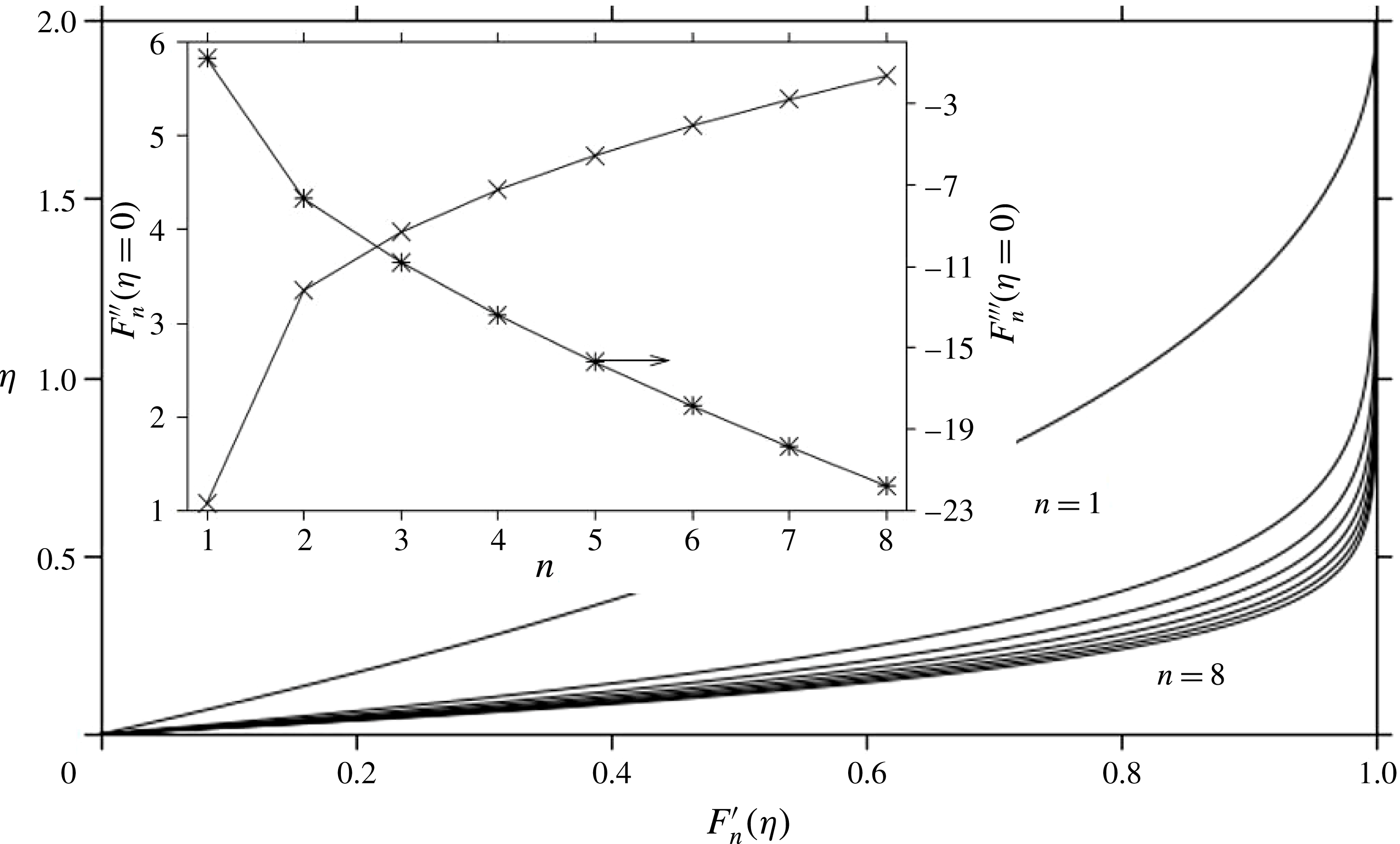
This is a two-point boundary-value problem, which is solved numerically for each mode separately. A finite-difference scheme with differed corrections (IMSL-DBVPFD) is used. Figure 3 depicts the profiles of
 $F_{n}^{\prime }(\unicode[STIX]{x1D702})$
for the first eight modes, which reflect a monotonic growth of
 $F_{n}(\unicode[STIX]{x1D702})$
and its derivatives. More importantly, we observe the significant departure of the function for the first mode (corresponding to
 $\unicode[STIX]{x1D6FD}_{1}=0.17$
) from the rest, which signals the dominance of the first mode on the velocity, as will be confirmed later (see table 1 in § 4). Given the physical significance of
 $F_{n}^{\prime \prime }(\unicode[STIX]{x1D702}=0)$
and
 $F_{n}^{\prime \prime \prime }(\unicode[STIX]{x1D702}=0)$
, and their relation to the shear stress at the wall and pressure respectively, we include their values in the inset of figure 3 as well as table 1. In particular, we find that
 $F_{n}^{\prime \prime }(\unicode[STIX]{x1D702}=0)>0$
and
 $F_{n}^{\prime \prime \prime }(\unicode[STIX]{x1D702}=0)<0$
for all modes, which indicates that the wall shear stress increases upon approaching the channel exit, with the pressure gradient becoming increasingly negative, as we shall see shortly (refer to expressions (3.41) and (3.42)).
The profiles of
 $F_{n}^{\prime }(\unicode[STIX]{x1D702})$
for the first eight modes. Also shown are the (discrete) values of
 $F_{n}^{\prime \prime }(\unicode[STIX]{x1D702}=0)$
and
 $F_{n}^{\prime \prime \prime }(\unicode[STIX]{x1D702}=0)$
in the inset. Successive points are joined for guidance.

Values for the first eight modes.

To the current order, the velocity components near the lower wall are then given by
 $$\begin{eqnarray}\displaystyle & \displaystyle u(\unicode[STIX]{x1D709},\unicode[STIX]{x1D702})=6\unicode[STIX]{x1D700}\unicode[STIX]{x1D702}(1-\unicode[STIX]{x1D700}\unicode[STIX]{x1D702})+\unicode[STIX]{x1D700}^{3}\mathop{\sum }_{n=1}^{\infty }\frac{A_{n}}{\unicode[STIX]{x1D6FD}_{n}}\text{e}^{\unicode[STIX]{x1D6FD}_{n}\unicode[STIX]{x1D709}}F_{n}^{\prime }(\unicode[STIX]{x1D702}), & \displaystyle\end{eqnarray}$$
 $$\begin{eqnarray}\displaystyle & \displaystyle w(\unicode[STIX]{x1D709},\unicode[STIX]{x1D702})=-\unicode[STIX]{x1D700}^{4}\mathop{\sum }_{n=1}^{\infty }A_{n}\text{e}^{\unicode[STIX]{x1D6FD}_{n}\unicode[STIX]{x1D709}}F_{n}(\unicode[STIX]{x1D702}). & \displaystyle\end{eqnarray}$$
The asymptote is then
 $u(\unicode[STIX]{x1D709},\unicode[STIX]{x1D702}\rightarrow \infty )\sim 6\unicode[STIX]{x1D700}\unicode[STIX]{x1D702}(1-\unicode[STIX]{x1D700}\unicode[STIX]{x1D702})+\unicode[STIX]{x1D700}^{3}\sum _{n=1}^{\infty }(A_{n}/\unicode[STIX]{x1D6FD}_{n})\text{e}^{\unicode[STIX]{x1D6FD}_{n}\unicode[STIX]{x1D709}}$
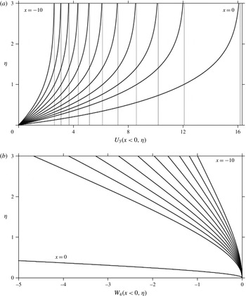
. Figure 4 depicts the flow development near the lower wall, where the profiles of the disturbances in velocity in the streamwise (figure 4
a) and transverse (figure 4
b) directions,
 $U_{3}(\unicode[STIX]{x1D709},\unicode[STIX]{x1D702})=\sum _{n=1}^{\infty }(A_{n}/\unicode[STIX]{x1D6FD}_{n})\text{e}^{\unicode[STIX]{x1D6FD}_{n}\unicode[STIX]{x1D709}}F_{n}^{\prime }(\unicode[STIX]{x1D702})$
and
 $W_{4}(\unicode[STIX]{x1D709},\unicode[STIX]{x1D702})=-\sum _{n=1}^{\infty }A_{n}\text{e}^{\unicode[STIX]{x1D6FD}_{n}\unicode[STIX]{x1D709}}F_{n}(\unicode[STIX]{x1D702})$
respectively, are shown at equal intervals for
 $-10<x<0$
. Both disturbances vanish exponentially in the limit
 $x\rightarrow -\infty$
. As expected, the asymptote, which reflects the extent of the (inviscid) character of the core flow, does not satisfy adherence at the lower (or upper) wall. Within the wall layer, the profiles exhibit an increase in shearing, confirming the increase in wall shear stress anticipated earlier. There is also a significant elongation as the fluid approaches the exit, which is particularly reflected in drastic departure in the
 $W_{4}(x=0,z)$
from zero.
Flow development near the lower wall. Streamwise (a) and transverse (b) velocity disturbance profiles are shown at equal intervals for
 $-10<x<0$
. Asymptotes are also shown for
 $U_{3}$
.

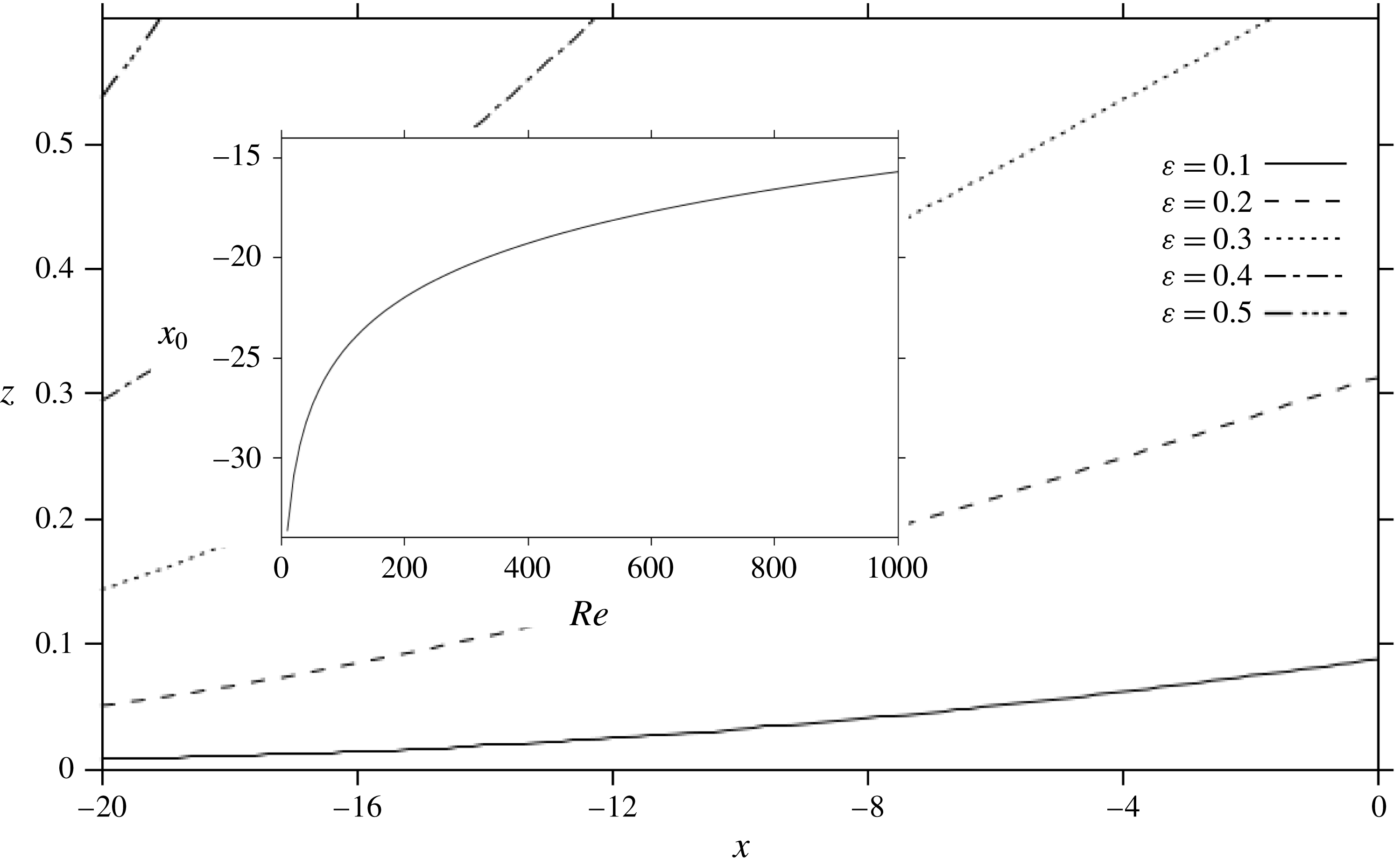
Figure 5 depicts the influence of inertia on the thickness of the lower-wall layer, which is estimated as the height reached when the relative difference between
 $u(\unicode[STIX]{x1D709},\unicode[STIX]{x1D702})$
and its asymptote is less than 1 %. In this case, we roughly have the following behaviour:
 $z\propto Re^{-1}\text{e}^{\unicode[STIX]{x1D6FD}_{1}x}$
for the boundary-layer thickness. Figure 5 indicates that, for any
 $\unicode[STIX]{x1D700}$
, the height increases rather rapidly with upstream distance. The behaviour is almost exponential, contrasting the much slower
 $\sqrt{x}$
behaviour typical of boundary-layer growth. The height of the lower layer can be rather significant, reaching 30 % into the channel gap for
 $\unicode[STIX]{x1D700}=0.3$
(
 $Re=37$
) and essentially vanishing for
 $\unicode[STIX]{x1D700}<0.1$
(
 $Re>1000$
). The onset position of the wall layer
 $x_{0}$
coincides with the disturbance of
 $\unicode[STIX]{x1D700}^{3}\sum _{n=1}^{\infty }(A_{n}/\unicode[STIX]{x1D6FD}_{n})\text{e}^{\unicode[STIX]{x1D6FD}_{n}\unicode[STIX]{x1D709}}$
from zero. Thus, keeping the dominant mode, and assuming the onset of the wall layer to coincide with a disturbance larger than
 $10^{-2}$
, we roughly have the following logarithmic dependence on
 $Re$
:
 $$\begin{eqnarray}\displaystyle x_{0}\simeq \frac{1}{\unicode[STIX]{x1D6FD}_{1}}\ln \left(0.01\frac{\unicode[STIX]{x1D6FD}_{1}}{A_{1}}Re^{2/3}\right), & & \displaystyle\end{eqnarray}$$
where
 $\unicode[STIX]{x1D6FD}_{1}=0.17$
and
 $A_{1}=2.43$
. The inset in figure 5 gives the onset position for
 $0<Re<1000$
. Obviously, the flow tends to retain its Poiseuille character closer to the exit for larger Reynolds number. We finally note that for very small
 $Re$
(a range that is not necessarily accurately treated in the current formulation), the upstream recovery distance is approximately 20 times the channel gap. Figure 5 also illustrates the extent of upstream influence, which, comparatively, is essentially absent for the flow over a mild constriction in a channel (Smith Reference Smith1976a
,Reference Smith
b
) and is manifested for severe constrictions (Smith Reference Smith1977, Reference Smith1979).
The influence of inertia on the height of the lower-wall layer, upstream of the channel exit (
 $x<0$
). The inset shows the logarithmic dependence on
 $Re$
of the onset position of the wall layer.

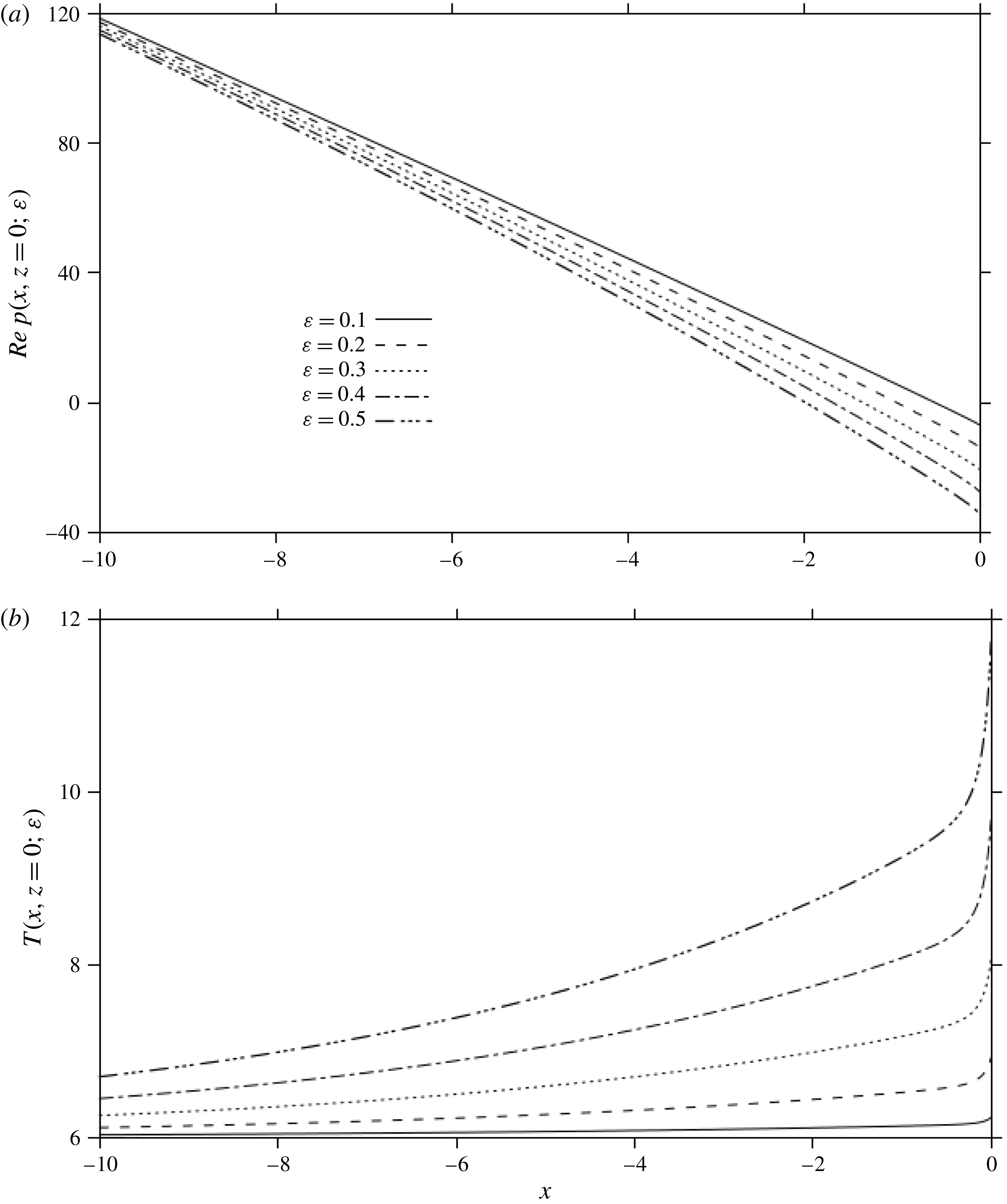
The influence of inertia on the pressure (a) and skin friction (b) along the lower wall.

Subject to its vanishing far upstream, the pressure correction becomes
 $P_{4}(x)=\sum _{n=1}^{\infty }(A_{n}/\unicode[STIX]{x1D6FD}_{n}^{2})\text{e}^{\unicode[STIX]{x1D6FD}_{n}x}F_{n}^{\prime \prime \prime }(\unicode[STIX]{x1D702}=0)$
. In this case, the pressure and wall shear stress are given by
 $$\begin{eqnarray}\displaystyle & \displaystyle p(\unicode[STIX]{x1D709},\unicode[STIX]{x1D702})=-12\unicode[STIX]{x1D700}^{3}\unicode[STIX]{x1D709}+\unicode[STIX]{x1D700}^{4}\mathop{\sum }_{n=1}^{\infty }\frac{A_{n}}{\unicode[STIX]{x1D6FD}_{n}^{2}}\text{e}^{\unicode[STIX]{x1D6FD}_{n}\unicode[STIX]{x1D709}}F_{n}^{\prime \prime \prime }(\unicode[STIX]{x1D702}=0), & \displaystyle\end{eqnarray}$$
 $$\begin{eqnarray}\displaystyle & \displaystyle \unicode[STIX]{x1D70F}(\unicode[STIX]{x1D709},\unicode[STIX]{x1D702}=0)=6+\unicode[STIX]{x1D700}^{2}\mathop{\sum }_{n=1}^{\infty }\frac{A_{n}}{\unicode[STIX]{x1D6FD}_{n}}\text{e}^{\unicode[STIX]{x1D6FD}_{n}\unicode[STIX]{x1D709}}F_{n}^{\prime \prime }(\unicode[STIX]{x1D702}=0). & \displaystyle\end{eqnarray}$$
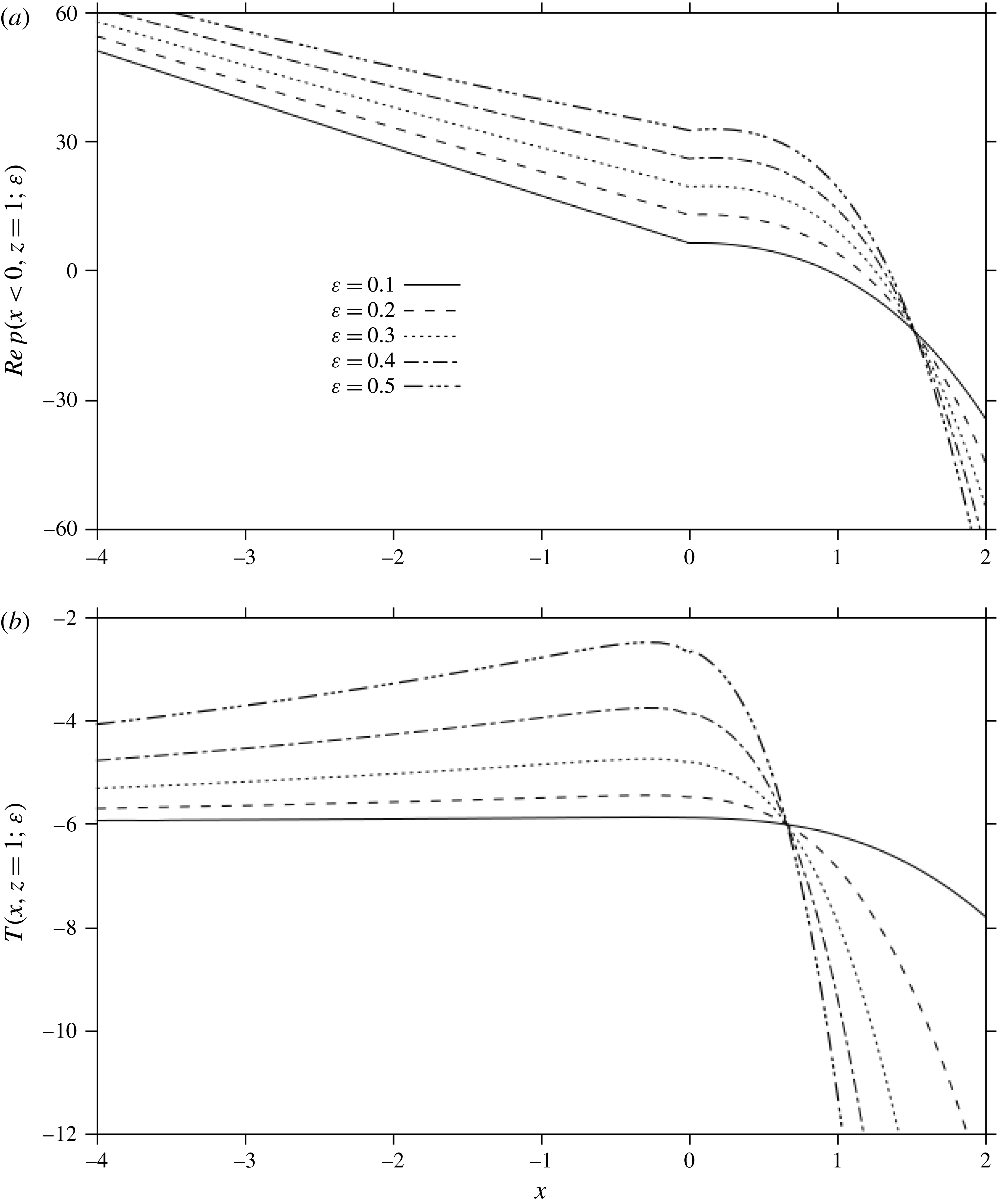
The shear stress at the wall turns out to be always positive (refer to the inset in figure 3 and table 1). Therefore, there is no possibility of separation upstream of the channel exit along the lower wall. Figure 6 illustrates the influence of inertia on the development of the pressure (figure 6
a) and the shear stress along the lower wall (figure 6
b) upstream of the channel exit. The pressure remains close to the Poiseuille level, decreasing essentially linearly all the way to the exit, but reaches a negative level at the exit. In contrast, the level of shearing increases rather rapidly for the range of Reynolds number reported in the figure, almost doubling for
 $\unicode[STIX]{x1D700}=0.5$
(
 $Re=8$
), reflecting the flattening of the velocity profile near the exit, as shown in figure 4. We observe that both the shear stress and the pressure are singular at
 $x=0$
, as the fluid moves along the lower wall, and emerges along the jet free surface, experiencing vanishing shear stress and pressure. However, upstream of the exit, the pressure and shear stress are well behaved.
3.3 The flow near the upper wall upstream and downstream of the channel exit
We now examine the boundary-layer structure near the infinite upper wall, upstream and downstream of the exit. In this case, the scaling in the transverse direction is changed by writing
 $$\begin{eqnarray}\displaystyle x=\unicode[STIX]{x1D709},\quad z=1-y=1-\unicode[STIX]{x1D700}\unicode[STIX]{x1D702}. & & \displaystyle\end{eqnarray}$$
Matching with the core flow suggests that
 $\unicode[STIX]{x1D713}\sim 1$
as
 $\unicode[STIX]{x1D702}\rightarrow \infty$
(see below). In this case, the balance between the convective and viscous terms leads to the following problem:
 $$\begin{eqnarray}\displaystyle & \displaystyle \unicode[STIX]{x1D713}_{\unicode[STIX]{x1D702}}\unicode[STIX]{x1D713}_{\unicode[STIX]{x1D709}\unicode[STIX]{x1D702}}-\unicode[STIX]{x1D713}_{\unicode[STIX]{x1D709}}\unicode[STIX]{x1D713}_{\unicode[STIX]{x1D702}\unicode[STIX]{x1D702}}=-\unicode[STIX]{x1D700}^{2}p_{\unicode[STIX]{x1D709}}-\unicode[STIX]{x1D700}^{2}\unicode[STIX]{x1D713}_{\unicode[STIX]{x1D702}\unicode[STIX]{x1D702}\unicode[STIX]{x1D702}}-\unicode[STIX]{x1D700}^{4}\unicode[STIX]{x1D713}_{\unicode[STIX]{x1D709}\unicode[STIX]{x1D709}\unicode[STIX]{x1D702}}, & \displaystyle\end{eqnarray}$$
 $$\begin{eqnarray}\displaystyle & \displaystyle \unicode[STIX]{x1D713}_{\unicode[STIX]{x1D702}}\unicode[STIX]{x1D713}_{\unicode[STIX]{x1D709}\unicode[STIX]{x1D709}}-\unicode[STIX]{x1D713}_{\unicode[STIX]{x1D709}}\unicode[STIX]{x1D713}_{\unicode[STIX]{x1D709}\unicode[STIX]{x1D702}}=p_{\unicode[STIX]{x1D702}}-\unicode[STIX]{x1D700}^{2}\unicode[STIX]{x1D713}_{\unicode[STIX]{x1D709}\unicode[STIX]{x1D702}\unicode[STIX]{x1D702}}-\unicode[STIX]{x1D700}^{4}\unicode[STIX]{x1D713}_{\unicode[STIX]{x1D709}\unicode[STIX]{x1D709}\unicode[STIX]{x1D709}}, & \displaystyle\end{eqnarray}$$
 $$\begin{eqnarray}\displaystyle \unicode[STIX]{x1D713}(\unicode[STIX]{x1D709},\unicode[STIX]{x1D702}=0)=1,\quad \unicode[STIX]{x1D713}_{\unicode[STIX]{x1D702}}(\unicode[STIX]{x1D709},\unicode[STIX]{x1D702}=0)=0,\quad \unicode[STIX]{x1D713}(\unicode[STIX]{x1D709}\rightarrow -\infty ,\unicode[STIX]{x1D702})\sim 1-3\unicode[STIX]{x1D700}^{2}\unicode[STIX]{x1D702}^{2}+2\unicode[STIX]{x1D700}^{3}\unicode[STIX]{x1D702}^{3}. & & \displaystyle \nonumber\\ \displaystyle & & \displaystyle\end{eqnarray}$$
The expansions of the streamfunction and pressure take the form
 $$\begin{eqnarray}\displaystyle & \displaystyle \unicode[STIX]{x1D713}(\unicode[STIX]{x1D709},\unicode[STIX]{x1D702})=\unicode[STIX]{x1D6F9}_{0}(\unicode[STIX]{x1D709},\unicode[STIX]{x1D702})+\unicode[STIX]{x1D700}\unicode[STIX]{x1D6F9}_{1}(\unicode[STIX]{x1D709},\unicode[STIX]{x1D702})+\unicode[STIX]{x1D700}^{2}\unicode[STIX]{x1D6F9}_{2}(\unicode[STIX]{x1D709},\unicode[STIX]{x1D702})+\unicode[STIX]{x1D700}^{3}\unicode[STIX]{x1D6F9}_{3}(\unicode[STIX]{x1D709},\unicode[STIX]{x1D702})+\unicode[STIX]{x1D700}^{4}\unicode[STIX]{x1D6F9}_{4}(\unicode[STIX]{x1D709},\unicode[STIX]{x1D702})+\cdots \,,\qquad & \displaystyle\end{eqnarray}$$
 $$\begin{eqnarray}\displaystyle & \displaystyle p(\unicode[STIX]{x1D709},\unicode[STIX]{x1D702})=P_{0}(\unicode[STIX]{x1D709},\unicode[STIX]{x1D702})+\unicode[STIX]{x1D700}P_{1}(\unicode[STIX]{x1D709},\unicode[STIX]{x1D702})+\unicode[STIX]{x1D700}^{2}P_{2}(\unicode[STIX]{x1D709},\unicode[STIX]{x1D702})+\cdots \,. & \displaystyle\end{eqnarray}$$
Near the upper wall, equation (4.1) may be written as
 $$\begin{eqnarray}\displaystyle \unicode[STIX]{x1D713}(x,z)=1-3y^{2}+2y^{3}+\unicode[STIX]{x1D700}^{3}[\unicode[STIX]{x1D713}_{3}(x,z=1)-y\unicode[STIX]{x1D713}_{3z}(x,z=1)+\cdots \,]. & & \displaystyle\end{eqnarray}$$
Clearly,
 $E_{0}\unicode[STIX]{x1D713}=1-3y^{2}+2y^{3}$
, so that
 $H_{3}E_{0}\unicode[STIX]{x1D713}=1-3\unicode[STIX]{x1D700}^{2}\unicode[STIX]{x1D702}^{2}+2\unicode[STIX]{x1D700}^{3}\unicode[STIX]{x1D702}^{3}$
. Moreover, from (3.45a
), we have
 $H_{3}\unicode[STIX]{x1D713}=\unicode[STIX]{x1D6F9}_{0}+\unicode[STIX]{x1D700}\unicode[STIX]{x1D6F9}_{1}+\unicode[STIX]{x1D700}^{2}\unicode[STIX]{x1D6F9}_{2}+\unicode[STIX]{x1D700}^{3}\unicode[STIX]{x1D6F9}_{3}$
. Setting
 $H_{3}E_{0}\unicode[STIX]{x1D713}=E_{0}H_{3}\unicode[STIX]{x1D713}$
, we deduce, as expected, that
 $\unicode[STIX]{x1D6F9}_{0}\sim 1,\unicode[STIX]{x1D6F9}_{1}\sim 0$
,
 $\unicode[STIX]{x1D6F9}_{2}\sim -3\unicode[STIX]{x1D702}^{2}$
and
 $\unicode[STIX]{x1D6F9}_{3}\sim 2\unicode[STIX]{x1D702}^{3}$
for large
 $\unicode[STIX]{x1D702}$
. In this case, it is not difficult to show that the solutions to
 $O(1),O(\unicode[STIX]{x1D700})$
,
 $O(\unicode[STIX]{x1D700}^{2})$
and
 $O(\unicode[STIX]{x1D700}^{3})$
, which satisfy the homogeneous conditions at the upper wall and far-upstream condition in (3.44c-e
), are
 $$\begin{eqnarray}\displaystyle \unicode[STIX]{x1D6F9}_{0}(\unicode[STIX]{x1D709},\unicode[STIX]{x1D702})=1,\quad P_{0}(\unicode[STIX]{x1D709},\unicode[STIX]{x1D702})=0,\quad \unicode[STIX]{x1D6F9}_{1}(\unicode[STIX]{x1D709},\unicode[STIX]{x1D702})=P_{1}(\unicode[STIX]{x1D709},\unicode[STIX]{x1D702})=0, & & \displaystyle\end{eqnarray}$$
 $$\begin{eqnarray}\displaystyle \unicode[STIX]{x1D6F9}_{2}(\unicode[STIX]{x1D709},\unicode[STIX]{x1D702})=-3\unicode[STIX]{x1D702}^{2},\quad P_{2}(\unicode[STIX]{x1D709},\unicode[STIX]{x1D702})=0, & & \displaystyle\end{eqnarray}$$
 $$\begin{eqnarray}\displaystyle \unicode[STIX]{x1D6F9}_{3}(\unicode[STIX]{x1D709},\unicode[STIX]{x1D702})=2\unicode[STIX]{x1D702}^{3},\quad P_{3}(\unicode[STIX]{x1D709},\unicode[STIX]{x1D702})=-12\unicode[STIX]{x1D709}. & & \displaystyle\end{eqnarray}$$
Thus, to
 $O(\unicode[STIX]{x1D700}^{3})$
, near the upper wall, as in the lower-wall layer, the flow retains its Poiseuille character. The flow field is then given by
 $$\begin{eqnarray}\displaystyle & \displaystyle \unicode[STIX]{x1D713}(\unicode[STIX]{x1D709},\unicode[STIX]{x1D702})=1-3\unicode[STIX]{x1D700}^{2}\unicode[STIX]{x1D702}^{2}+2\unicode[STIX]{x1D700}^{3}\unicode[STIX]{x1D702}^{3}+\unicode[STIX]{x1D700}^{4}\unicode[STIX]{x1D6F9}_{4}(\unicode[STIX]{x1D709},\unicode[STIX]{x1D702})+O(\unicode[STIX]{x1D700}^{5}), & \displaystyle\end{eqnarray}$$
 $$\begin{eqnarray}\displaystyle & \displaystyle p(\unicode[STIX]{x1D709},\unicode[STIX]{x1D702})=-12\unicode[STIX]{x1D700}^{3}x+\unicode[STIX]{x1D700}^{4}P_{4}(\unicode[STIX]{x1D709},\unicode[STIX]{x1D702})+O(\unicode[STIX]{x1D700}^{5}), & \displaystyle\end{eqnarray}$$
 $$\begin{eqnarray}\displaystyle & \displaystyle u(\unicode[STIX]{x1D709},\unicode[STIX]{x1D702})=6\unicode[STIX]{x1D700}\unicode[STIX]{x1D702}(1-\unicode[STIX]{x1D700}\unicode[STIX]{x1D702})-\unicode[STIX]{x1D700}^{3}\unicode[STIX]{x1D6F9}_{4\unicode[STIX]{x1D702}}(\unicode[STIX]{x1D709},\unicode[STIX]{x1D702})+O(\unicode[STIX]{x1D700}^{4}), & \displaystyle\end{eqnarray}$$
 $$\begin{eqnarray}\displaystyle & \displaystyle w(\unicode[STIX]{x1D709},\unicode[STIX]{x1D702})=-\unicode[STIX]{x1D700}^{4}\unicode[STIX]{x1D6F9}_{4\unicode[STIX]{x1D709}}(\unicode[STIX]{x1D709},\unicode[STIX]{x1D702})+O(\unicode[STIX]{x1D700}^{5}), & \displaystyle\end{eqnarray}$$
 $$\begin{eqnarray}\displaystyle & \displaystyle \unicode[STIX]{x1D70F}(\unicode[STIX]{x1D709},\unicode[STIX]{x1D702})=-6(1-\unicode[STIX]{x1D700}\unicode[STIX]{x1D702})+\unicode[STIX]{x1D700}^{2}\unicode[STIX]{x1D6F9}_{4\unicode[STIX]{x1D702}\unicode[STIX]{x1D702}}(\unicode[STIX]{x1D709},\unicode[STIX]{x1D702})+O(\unicode[STIX]{x1D700}^{3}). & \displaystyle\end{eqnarray}$$
At this stage, we need to determine the outer limit
 $\unicode[STIX]{x1D713}_{3}(x,z\rightarrow 1)$
for the core flow problem. To this end, we note first from (3.46) that
 $H_{3}E_{3}\unicode[STIX]{x1D713}=1-3y^{2}+2y^{3}+\unicode[STIX]{x1D700}^{3}\unicode[STIX]{x1D713}_{3}(x,z=1)$
, which must match with
 $E_{3}H_{3}\unicode[STIX]{x1D713}=1-3y^{2}+2y^{3}$
, yielding (for any
 $x$
)
 $$\begin{eqnarray}\displaystyle \unicode[STIX]{x1D713}_{3}(x,z=1)=0, & & \displaystyle\end{eqnarray}$$
which is the condition needed to determine the core flow upstream and downstream of the channel exit (refer to problem (4.5) in the next section).
We next consider the problem for
 $\unicode[STIX]{x1D6F9}_{4}$
and
 $P_{4}$
, which is similar to (3.36) both upstream and downstream of the channel exit, but is considerably more difficult for
 $x>0$
. For any
 $x$
, upon eliminating the pressure, the governing equation and upper-wall conditions for
 $\unicode[STIX]{x1D6F9}_{4}(\unicode[STIX]{x1D709},\unicode[STIX]{x1D702})$
become
 $$\begin{eqnarray}\displaystyle \unicode[STIX]{x1D6F9}_{4\unicode[STIX]{x1D702}\unicode[STIX]{x1D702}\unicode[STIX]{x1D702}\unicode[STIX]{x1D702}}=6\unicode[STIX]{x1D702}\unicode[STIX]{x1D6F9}_{4\unicode[STIX]{x1D709}\unicode[STIX]{x1D702}\unicode[STIX]{x1D702}},\quad \unicode[STIX]{x1D6F9}_{4}(\unicode[STIX]{x1D709},\unicode[STIX]{x1D702}=0)=\unicode[STIX]{x1D6F9}_{4\unicode[STIX]{x1D702}}(\unicode[STIX]{x1D709},\unicode[STIX]{x1D702}=0)=0. & & \displaystyle\end{eqnarray}$$
In addition, two boundary conditions are needed. However, they depend on whether the upper-wall layer lies upstream or downstream of the channel exit. For any
 $x$
, we have
 $H_{4}E_{3}\unicode[STIX]{x1D713}=1-3y^{2}+2y^{3}-\unicode[STIX]{x1D700}^{3}y\unicode[STIX]{x1D713}_{3z}(x,z=1)$
, which must match with
 $E_{3}H_{4}\unicode[STIX]{x1D713}=1-3y^{2}+2y^{3}+\unicode[STIX]{x1D700}^{4}\unicode[STIX]{x1D6F9}_{4}$
, yielding the condition
 $$\begin{eqnarray}\displaystyle \unicode[STIX]{x1D6F9}_{4}(\unicode[STIX]{x1D709},\unicode[STIX]{x1D702}\rightarrow \infty )\sim -\unicode[STIX]{x1D702}\unicode[STIX]{x1D713}_{3z}(x,z=1). & & \displaystyle\end{eqnarray}$$
We observe that
 $\unicode[STIX]{x1D713}_{3z}(x,z=1)$
is not the same for
 $x<0$
and
 $x>0$
.
3.3.1 The flow near the upper wall upstream of the channel exit
$(x<0)$

Upstream of the channel exit, the disturbance in the core streamfunction is deduced from (4.9) as
 $\unicode[STIX]{x1D713}_{3}(x<0,z)=\sum _{n=1}^{\infty }(A_{n}/\unicode[STIX]{x1D6FD}_{n})\text{e}^{\unicode[STIX]{x1D6FD}_{n}x}V_{n}(z)$
. In this case, the matching condition (3.53) and the vanishing of the disturbance far upstream must apply. As will be shown in § 4, it will turn out that
 $V_{n}^{\prime }(z=1)=(-1)^{n}$
. Consequently, the two conditions read
 $$\begin{eqnarray}\displaystyle \unicode[STIX]{x1D6F9}_{4\unicode[STIX]{x1D702}}(\unicode[STIX]{x1D709}<0,\unicode[STIX]{x1D702}\rightarrow \infty )\sim -\mathop{\sum }_{n=1}^{\infty }(-1)^{n}\frac{A_{n}}{\unicode[STIX]{x1D6FD}_{n}}\text{e}^{\unicode[STIX]{x1D6FD}_{n}\unicode[STIX]{x1D709}},\quad \unicode[STIX]{x1D6F9}_{4}(\unicode[STIX]{x1D709}\rightarrow -\infty ,\unicode[STIX]{x1D702})\sim 0. & & \displaystyle\end{eqnarray}$$
We proceed as before to solve (3.52) subject to (3.54) by seeking a solution of the form
 $\unicode[STIX]{x1D6F9}_{4}(\unicode[STIX]{x1D709}<0,\unicode[STIX]{x1D702})=-\sum _{n=1}^{\infty }(-1)^{n}(A_{n}/\unicode[STIX]{x1D6FD}_{n})\text{e}^{\unicode[STIX]{x1D6FD}_{n}\unicode[STIX]{x1D709}}F_{n}(\unicode[STIX]{x1D702})$
, in terms of the same functions
 $F_{n}(\unicode[STIX]{x1D702})$
that are governed by (3.38). In this case, the velocity components are given by
 $$\begin{eqnarray}\displaystyle & \displaystyle u(\unicode[STIX]{x1D709}<0,\unicode[STIX]{x1D702})=6\unicode[STIX]{x1D700}\unicode[STIX]{x1D702}(1-\unicode[STIX]{x1D700}\unicode[STIX]{x1D702})+\unicode[STIX]{x1D700}^{3}\mathop{\sum }_{n=1}^{\infty }\frac{A_{n}}{\unicode[STIX]{x1D6FD}_{n}}(-1)^{n}\text{e}^{\unicode[STIX]{x1D6FD}_{n}\unicode[STIX]{x1D709}}F_{n}^{\prime }(\unicode[STIX]{x1D702}), & \displaystyle\end{eqnarray}$$
 $$\begin{eqnarray}\displaystyle & \displaystyle w(\unicode[STIX]{x1D709}<0,\unicode[STIX]{x1D702})=\unicode[STIX]{x1D700}^{4}\mathop{\sum }_{n=1}^{\infty }A_{n}(-1)^{n}\text{e}^{\unicode[STIX]{x1D6FD}_{n}\unicode[STIX]{x1D709}}F_{n}(\unicode[STIX]{x1D702}). & \displaystyle\end{eqnarray}$$
Comparison with the velocity components (3.39) at the lower wall reveals clearly the break in the symmetry, especially through the change in sign in the (dominant) first mode for
 $u$
.
3.3.2 The flow near the upper wall downstream of the channel exit
$(x>0)$

Downstream of the channel exit, the flow near the upper wall must match the core flow as well as the upstream flow at the exit:
 $\unicode[STIX]{x1D6F9}_{4}(\unicode[STIX]{x1D709}=0^{-},\unicode[STIX]{x1D702})=\unicode[STIX]{x1D6F9}_{4}(\unicode[STIX]{x1D709}=0^{+},\unicode[STIX]{x1D702})$
. This provides the two additional conditions needed to ensure the well-posedness of problem (3.52) for
 $x>0$
. Noting that
 $\unicode[STIX]{x1D713}_{3}(x>0,z)=2xU_{0}(z)-(5/3)x^{3}u_{0}(z)+\sum _{n=1}^{\infty }(A_{n}/\unicode[STIX]{x1D6FD}_{n})\text{e}^{-\unicode[STIX]{x1D6FD}_{n}x}V_{n}(z)$
from (4.20), and recalling (3.53), the two conditions become
 $$\begin{eqnarray}\displaystyle & \displaystyle \unicode[STIX]{x1D6F9}_{4\unicode[STIX]{x1D702}}(\unicode[STIX]{x1D709}>0,\unicode[STIX]{x1D702}\rightarrow \infty )\sim -10\unicode[STIX]{x1D709}^{3}-\mathop{\sum }_{n=1}^{\infty }(-1)^{n}\frac{A_{n}}{\unicode[STIX]{x1D6FD}_{n}}\text{e}^{-\unicode[STIX]{x1D6FD}_{n}\unicode[STIX]{x1D709}}, & \displaystyle\end{eqnarray}$$
 $$\begin{eqnarray}\displaystyle & \displaystyle \unicode[STIX]{x1D6F9}_{4\unicode[STIX]{x1D702}}(\unicode[STIX]{x1D709}=0^{+},\unicode[STIX]{x1D702})=-\mathop{\sum }_{n=1}^{\infty }\frac{A_{n}}{\unicode[STIX]{x1D6FD}_{n}}(-1)^{n}F_{n}(\unicode[STIX]{x1D702}). & \displaystyle\end{eqnarray}$$
We note that
 $U_{0}^{\prime }(z=1)=0$
is used. Problem (3.52) subject to (3.56) is less obvious to solve than for the flow upstream since the problem does not allow separation of variables due to the presence of the cubic
 $\unicode[STIX]{x1D709}$
-dependent terms. We implement an explicit finite-difference discretization in the streamwise direction, coupled with a numerical integration of the resulting two-point boundary-value problem in the transverse direction at each
 $\unicode[STIX]{x1D709}=\unicode[STIX]{x1D709}_{i}$
position. Thus, upon letting
 $\unicode[STIX]{x1D6E5}\equiv \unicode[STIX]{x1D709}_{i}-\unicode[STIX]{x1D709}_{i-1}$
and
 $K_{i}(\unicode[STIX]{x1D702})\equiv \unicode[STIX]{x1D6F9}_{4}(\unicode[STIX]{x1D709}=\unicode[STIX]{x1D709}_{i},\unicode[STIX]{x1D702})$
, the discretized problem becomes
 $$\begin{eqnarray}\displaystyle K_{i}^{\prime \prime \prime \prime }=\frac{6}{\unicode[STIX]{x1D6E5}}\unicode[STIX]{x1D702}(K_{i}^{\prime \prime }-K_{i-1}^{\prime \prime }),\quad K_{i}(0)=K_{i}^{\prime }(0)=0,\quad K_{i}^{\prime \prime }(\infty )\sim 0, & & \displaystyle\end{eqnarray}$$
 $$\begin{eqnarray}\displaystyle K_{i}^{\prime }(\infty )\sim -10\unicode[STIX]{x1D709}_{i}^{3}-\mathop{\sum }_{n=1}^{\infty }\frac{A_{n}}{\unicode[STIX]{x1D6FD}_{n}}(-1)^{n}\text{e}^{-\unicode[STIX]{x1D6FD}_{n}\unicode[STIX]{x1D709}_{i}},\quad K_{0}^{\prime \prime }(\unicode[STIX]{x1D702})=-\mathop{\sum }_{n=1}\frac{A_{n}}{\unicode[STIX]{x1D6FD}_{n}}(-1)^{n}F_{n}^{\prime \prime }(\unicode[STIX]{x1D702}).\qquad & & \displaystyle\end{eqnarray}$$
Problem (3.57) was solved using the IMSL-DBVP routine. The step size
 $\unicode[STIX]{x1D6E5}$
was typically taken equal to 0.01, which turned out to be sufficiently small for stability and convergence. The far conditions were reached essentially for
 $\unicode[STIX]{x1D702}<10$
(see figure 7 below). Clearly, from the first condition in (3.57d,e
), we expect the flow to deviate rather significantly as the exit is traversed; as the exponential terms decay, the cubic
 $\unicode[STIX]{x1D709}$
-dependent term becomes increasingly dominant with distance.
The variation of the streamfunction disturbance
 $\unicode[STIX]{x1D6F9}_{4}(x,\unicode[STIX]{x1D702})$
and its derivatives across the upper-wall layer downstream of the channel exit for
 $0\leqslant x\leqslant 1$
. Profiles are shown at equal intervals of 0.1.

Figure 7 shows the behaviour of
 $\unicode[STIX]{x1D6F9}_{4}(\unicode[STIX]{x1D709},\unicode[STIX]{x1D702})$
and its derivatives at equal interval positions between the exit (
 $x=0$
) and
 $x=1$
. Figure 7(a) shows that linear behaviour, with constant slope given in (3.57d,e
), is reached at a distance increasingly farther from the upper wall (larger
 $\unicode[STIX]{x1D702}$
) as the fluid moves further downstream (as
 $x$
increases), with significant decrease in slope, which is also obvious from figure 7(b). There is a significant saturation near
 $x=0$
, which suggests a slow departure in streamwise and transverse velocity components just downstream of the exit. In contrast, figure 7(c,d) suggests that the wall shear stress and pressure tend to depart more rapidly when the exit is crossed. Overall, the flow experiences an increasingly larger departure further downstream. At some distance,
 $\unicode[STIX]{x1D6F9}_{4}(\unicode[STIX]{x1D709},\unicode[STIX]{x1D702})$
and its derivatives change sign (not necessarily at the same location) at the upper wall and below. Figure 7(a) and expression (3.50d
) indicate that the transverse velocity component remains positive upstream and downstream, strengthening with distance along the upper wall, reflecting a positive and strong elongation rate
 $2u_{x}$
, which is also evident from figure 7(b) and expression (3.50b
). The elongation rate is always positive and increases with downstream distance. This behaviour contrasts sharply that of a wall jet emerging into an ambient fluid, which weakens near the wall as it exits the channel (Levin et al.
Reference Levin, Chernoray, Fdahl and Henningson2005; Peters et al.
Reference Peters, Rupel, Javili and Kunkel2008). The flow in the present free-surface wall jet will have to eventually weaken when it expands further downstream, to behave then like a wall jet. The monotonicity of the velocity does not extend to the wall shear stress. The change in sign in figure 7(c), along with expression (3.50e
), suggests that
 $\unicode[STIX]{x1D70F}(\unicode[STIX]{x1D709}>0,\unicode[STIX]{x1D702}=0)$
decreases with distance near the exit but increases again at approximately
 $x=0.7$
. A maximum in wall shear stress is therefore anticipated, as we shall see below, and contrasts the monotonicity along the lower wall (see figure 6). Finally, figure 7(d) illustrates the behaviour of the pressure gradient at and near the upper wall, which may be written as
 $$\begin{eqnarray}\displaystyle Re\,p^{\prime }(\unicode[STIX]{x1D709}>0)=-12-\unicode[STIX]{x1D700}\unicode[STIX]{x1D6F9}_{4\unicode[STIX]{x1D702}\unicode[STIX]{x1D702}\unicode[STIX]{x1D702}}(\unicode[STIX]{x1D709},\unicode[STIX]{x1D702}=0). & & \displaystyle\end{eqnarray}$$
Close to the exit, the pressure gradient may or may not remain negative depending on the inertia level. However, an adverse gradient cannot occur here since, given that
 $\unicode[STIX]{x1D6F9}_{4\unicode[STIX]{x1D702}\unicode[STIX]{x1D702}\unicode[STIX]{x1D702}}(\unicode[STIX]{x1D709}=0,\unicode[STIX]{x1D702}=0)=7.38$
,
 $\unicode[STIX]{x1D700}$
needs to be larger than 1.62 or
 $Re<0.23$
, a range that is clearly not covered by the present formulation. However, as we shall see next, despite the apparent unfavourable adverse pressure, separation can still be envisaged.
Pressure (a) and skin friction (b) along the upper wall downstream of the channel exit for various levels of inertia.

Figure 8 displays the influence of inertia on the pressure and skin friction along the upper wall upstream and downstream of the exit. As in the case along the lower wall, the pressure retains a predominantly linear behaviour upstream of the exit, but develops at a milder rate compared with the pressure along the lower wall (figure 6). In contrast to the pressure near the lower wall, the pressure near the upper wall remains positive for
 $x<0$
(figure 8
a), reflecting the break in symmetry and the extent of upstream influence. For
 $x>0$
, the pressure continues to drop with
 $x$
, but at a slower rate. It should be recalled that a positive pressure gradient is highly unlikely unless inertia is very low
 $(\unicode[STIX]{x1D700}>1.62)$
. Nevertheless, the adverse pressure at the exit can be expected given the strong elongational effect and surface curvature at the exit (see figure 2
a,b), and is typically encountered in coating flow, in particular blade coating (see, for instance, figure 9 in Iliopoulos & Scriven (Reference Iliopoulos and Scriven2005)). We note that, in coating flow, the pressure growth is halted by the movement of the web or substrate (upper wall in figure 1) and slip (see figure 8 in Schmidt, Schlosser & Schollmeyer (Reference Schmidt, Schlosser and Schollmeyer2009)); the pressure becomes atmospheric. Despite the absence of adverse pressure, there is a surge in shear stress along the wall, as figure 8(b) suggests. More importantly, shearing leads potentially to flow separation at a position increasingly closer to the channel exit as inertia decreases. This can be seen by examining expression (3.29), and it can be established that the shear stress becomes positive at a distance when
 $$\begin{eqnarray}\displaystyle \unicode[STIX]{x1D70F}(\unicode[STIX]{x1D709},\unicode[STIX]{x1D702}=0)=-6+\unicode[STIX]{x1D700}^{2}\unicode[STIX]{x1D6F9}_{4\unicode[STIX]{x1D702}\unicode[STIX]{x1D702}}(\unicode[STIX]{x1D709},\unicode[STIX]{x1D702}=0) & & \displaystyle\end{eqnarray}$$
vanishes. Consequently, a positive shear stress occurs first at the exit when (from figure 7
c)
 $\unicode[STIX]{x1D700}=\sqrt{6/(\unicode[STIX]{x1D6F9}_{4\unicode[STIX]{x1D702}\unicode[STIX]{x1D702}}(\unicode[STIX]{x1D709}=0,\unicode[STIX]{x1D702}=0))}=0.65$
or
 $Re=3.56$
. Additional calculations for
 $\unicode[STIX]{x1D700}>0.65$
(not shown here) suggest that the flow indeed separates near the exit and reattaches downstream as a result of jet expansion. In this case, the maximum in wall shear stress is positive (refer again to figure 8
b). This behaviour is reminiscent of the flow downstream of a localized constriction (Smith Reference Smith1976a
,Reference Smith
b
). For the present jet flow, the shear stress decreases with downstream distance at an increasingly larger rate for lower inertia (see figure 8
b). The non-monotonic response of the shear stress, with respect to both distance and Reynolds number, should help to explain the wide variation of the skin friction measured in experiments on wall jets (Maki Reference Maki1983). The increase in wall shear rate is a reflection of velocity flattening near the upper wall as the jet expands. This is discussed further next.
The evolution of the velocity profile in the upper-wall layer is illustrated in figure 9 for
 $\unicode[STIX]{x1D700}=0.3$
(
 $Re=37$
). The profiles are shown at different positions
 $(0\leqslant x\leqslant 2)$
downstream of the exit. At the exit (
 $x=0$
), the flow retains predominantly its Poiseuille character. Further downstream, the velocity gradually increases near the upper wall (as the jet contracts), accompanied by an increase in elongation effect with distance, which is reflected by the widening of successive profiles. This behaviour is atypical of wall-jet flow (Glauert Reference Glauert1956; Peters et al.
Reference Peters, Rupel, Javili and Kunkel2008). When a wall jet emerges from a channel into the ambient fluid, it expands immediately at the exit and continues to expand downstream. In contrast, the present free-surface wall jet experiences a contraction near the exit, as shown in figure 2(a). Eventually, it expands at a rate that is larger for lower inertial flow. It is the contraction that is causing the flow to strengthen near the upper wall as shown in figure 9, and reflected in the sharp drop in wall shear stress in figure 8(b). Eventually, the flow begins to weaken further downstream, with the shear stress levelling off and increasing with distance.
Streamwise velocity profiles in the upper-wall layer at different downstream positions at equal intervals between the channel exit at
 $x=0$
and
 $x=1$
.

Finally, we observe that, regardless of the level of inertia, the upper-wall layer and the free-surface layer eventually interact at some distance downstream of the channel exit, which we now estimate. We have already established the growths of the free-surface and upper-wall layers to be
 $\unicode[STIX]{x1D700}x^{1/3}$
and
 $\unicode[STIX]{x1D700}^{3}x^{3}$
respectively. Assuming that interaction occurs when the two layers are of the same order of thickness, this yields a distance
 $x=O(\unicode[STIX]{x1D700}^{-2/4})$
. Interestingly, this distance is smaller than
 $O(\unicode[STIX]{x1D700}^{-3})$
, which is the order of the distance that ensures the uniformity of expansion (3.26). We can therefore conclude that the interaction of the two layers occurs at a distance shorter than the location of the maximum in the jet surface predicted by (3.26) and illustrated in figure 2.
4 The flow in the core layer (inside and outside the channel)
In the core region, which is far from both
 $z=0$
and
 $z=1$
, the solution of equations (2.2) is sought subject to conditions (2.3) and (2.4). Although the treatment is similar to the case of a free jet (Tillett Reference Tillett1968; Khayat Reference Khayat2014), the current solution is more challenging for the downstream flow. The contributing terms that ensure the satisfaction of condition (3.13) do not reduce to a simple
 $z$
-dependent term. We refer the reader to expression (4.15) in Tillett (Reference Tillett1968) and the term
 $V_{0}(z)$
in question therein. This departure will be emphasized in the current paper in § 4.2 below. As in the case of the free jet,
 $\unicode[STIX]{x1D713}$
and
 $p$
are represented by the following outer expansions:
 $$\begin{eqnarray}\displaystyle & \displaystyle \unicode[STIX]{x1D713}(x,z)=\unicode[STIX]{x1D713}_{0}(x,z)+\unicode[STIX]{x1D700}\unicode[STIX]{x1D713}_{1}(x,z)+\cdots \,, & \displaystyle\end{eqnarray}$$
 $$\begin{eqnarray}\displaystyle & \displaystyle p(x,z)=p_{0}(x,z)+\unicode[STIX]{x1D700}p_{1}(x,z)+\cdots \,. & \displaystyle\end{eqnarray}$$
Here, we recall that
 $\unicode[STIX]{x1D713}_{0}=3z^{2}-2z^{3}$
is just the basic Poiseuille streamfunction given in (2.1);
 $\unicode[STIX]{x1D713}_{m}(x,z)$
for
 $m>0$
are higher-order terms that represent the deviation from the base flow due to its interaction between the core and boundary layers. The character of the base flow is similar to that arising for the laminar flow of a free jet (Tillett Reference Tillett1968) and channel or tube flow with constriction (Smith Reference Smith1976a
,Reference Smith
b
, Reference Smith1979) at high Reynolds number. In such cases, as well, the fully developed (Poiseuille) profile is the flow to leading order. Smith examined the flow for fine and moderate (Smith Reference Smith1976a
,Reference Smith
b
) as well as severe (Smith Reference Smith1979) constrictions. The severity of the constriction is reflected in the characteristic slope of the obstacle, which is of
 $O(Re^{-1/3})$
and
 $O(Re^{-1/6})$
for fine and moderate constrictions respectively. Here,
 $Re$
is Smith’s Reynolds number based on the tube diameter and the maximum velocity. In such situations, there occurs virtually no nonlinear upstream influence of the obstacle, and the core flow is just an inviscid rotational perturbation of the base Poiseuille flow. As it turns out, this is also the situation in the current problem, where the contraction of the flow constitutes a fine to moderate constriction. The core motion outside the inner and outer layers is of the inviscid elliptic, but linear, kind.
In contrast, in a severe constriction, where the obstacle slope is of
 $O(1)$
, there is significant upstream influence on the core flow. As mentioned earlier, this level of constriction severity does not correspond to the current problem. It should be noted that the flow field expansion takes the same form regardless of the constriction level of severity. Thus, Smith’s (Reference Smith1979) expansion (2.1) for the flow with severe constriction is the same as the current expansion (4.1) above. However, in contrast to (4.1), Smith’s leading-order terms in (2.1) do not exactly correspond to fully developed flow, but still satisfy the inviscid equations of motion. Free-streamline theory was adopted by Smith, which is believed to yield the proper inviscid limiting form of the Navier–Stokes equations (Smith Reference Smith1979).
Since the governing equations are elliptic (in
 $x$
), the deviation from the Poiseuille flow will extend also to the region
 $x<0$
in the channel. Based on these assumptions, upon inserting expressions (4.1) into equations (2.2), a hierarchy of equations is obtained to each order. To leading order,
 $p_{0}(x,z)=0$
. For
 $m=1$
and 2, the matching conditions obtained in §§ 3.1 and 3.3, and the condition
 $\unicode[STIX]{x1D713}_{m>0}(x\rightarrow -\infty ,z)\sim 0$
, lead to the vanishing of the streamfunction and pressure everywhere. More explicitly,
 $$\begin{eqnarray}\displaystyle \unicode[STIX]{x1D713}_{1}(x,z)=\unicode[STIX]{x1D713}_{2}(x,z)=p_{1}(x,z)=p_{2}(x,z)=0. & & \displaystyle\end{eqnarray}$$
To next order,
 $m=3$
, equations (2.2) lead to
 $$\begin{eqnarray}\displaystyle & \displaystyle \unicode[STIX]{x1D713}_{0z}\unicode[STIX]{x1D713}_{3xz}-\unicode[STIX]{x1D713}_{0zz}\unicode[STIX]{x1D713}_{3x}=-p_{3x}-12, & \displaystyle\end{eqnarray}$$
 $$\begin{eqnarray}\displaystyle & \displaystyle \unicode[STIX]{x1D713}_{0z}\unicode[STIX]{x1D713}_{3xx}=p_{3z}. & \displaystyle\end{eqnarray}$$
Upon eliminating
 $p_{3}$
from (4.4a
) and (4.4b
), the following equation is obtained for
 $\unicode[STIX]{x1D713}_{3}$
:
 $$\begin{eqnarray}\displaystyle \unicode[STIX]{x1D6FB}^{2}\unicode[STIX]{x1D713}_{3x}-\frac{\unicode[STIX]{x1D713}_{0zzz}}{\unicode[STIX]{x1D713}_{0z}}\unicode[STIX]{x1D713}_{3x}=0, & & \displaystyle\end{eqnarray}$$
where
 $\unicode[STIX]{x1D6FB}^{2}=\unicode[STIX]{x2202}^{2}/\unicode[STIX]{x2202}x^{2}+\unicode[STIX]{x2202}^{2}/\unicode[STIX]{x2202}z^{2}$
. Noting that
 $w_{3}=-\unicode[STIX]{x1D713}_{3x}$
, and using expression (2.1), we obtain the following boundary-value problem for
 $-\infty \leqslant x\leqslant \infty$
and
 $0\leqslant z\leqslant 1$
:
 $$\begin{eqnarray}\displaystyle & \displaystyle \unicode[STIX]{x1D6FB}^{2}w_{3}-\frac{u_{0}^{\prime \prime }}{u_{0}}w_{3}=0, & \displaystyle\end{eqnarray}$$
 $$\begin{eqnarray}\displaystyle & \displaystyle \left.\begin{array}{@{}ll@{}}w_{3}(-\infty <x<\infty ,z\rightarrow 1)\sim 0, & w_{3}(x<0,z\rightarrow 0)\sim 0,\\ w_{3}(x>0,z\rightarrow 0)\sim -2, & w_{3}\quad \text{bounded as }|x|\rightarrow \infty .\end{array}\right\} & \displaystyle\end{eqnarray}$$
These conditions are derived from (3.13), (3.19) and (3.40), which were obtained by matching the flow fields between the core and wall layers. The solution of problem (4.6) does not vanish given the non-homogeneity of the boundary conditions. So far, the formulation in this section has been common to both core regions inside and outside the channel. Although the flow fields in these two regions will have to match at the channel exit (
 $x=0$
), they can be conveniently examined separately.
4.1 The flow in the core layer upstream of the channel exit
Consider now the core flow in the region inside the channel
 $(x<0)$
. The solution of problem (4.6) is written as (Tillett Reference Tillett1968)
 $$\begin{eqnarray}\displaystyle w_{3}(x<0,z)=-\unicode[STIX]{x1D713}_{3x}(x<0,z)=-\mathop{\sum }_{n=1}^{\infty }A_{n}\text{e}^{\unicode[STIX]{x1D6FD}_{n}x}V_{n}(z). & & \displaystyle\end{eqnarray}$$
The shape functions
 $V_{n}$
are different from those for a free jet, and are governed by the following eigenvalue problem:
 $$\begin{eqnarray}\displaystyle V_{n}^{\prime \prime }+\left(\unicode[STIX]{x1D6FD}_{n}^{2}-\frac{u_{0}^{\prime \prime }}{u_{0}}\right)V_{n}=0,\quad V_{n}(0)=V_{n}(1)=0, & & \displaystyle\end{eqnarray}$$
which is solved subject to the additional boundary condition
 $V_{n}^{\prime }(0)=1$
. In this case,
 $V_{n}^{\prime \prime }(0)=-2$
and
 $V_{n}^{\prime \prime }(1)=2V_{n}^{\prime }(1)$
. In addition, the slope at the boundary turns out to be
 $V_{n}^{\prime }(1)=(-1)^{n}$
, which is established numerically (we could not confirm it analytically). Table 1 shows the eigenvalues for the first eight modes. Also included in the table are the corresponding values of the expansion coefficients
 $A_{n}$
(to be determined shortly), and the values of
 $F_{n}^{\prime \prime }(0)$
and
 $F_{n}^{\prime \prime \prime }(0)$
(determined earlier in § 3).
The streamfunction is obtained by integrating expression (4.7) subject to
 $\unicode[STIX]{x1D713}_{3}(x\rightarrow -\infty ,z)=0$
, leading to
 $$\begin{eqnarray}\displaystyle & \displaystyle \unicode[STIX]{x1D713}(x<0,z)=3z^{2}-2z^{3}+\unicode[STIX]{x1D700}^{3}\mathop{\sum }_{n=1}^{\infty }\frac{A_{n}}{\unicode[STIX]{x1D6FD}_{n}}\text{e}^{\unicode[STIX]{x1D6FD}_{n}x}V_{n}(z), & \displaystyle\end{eqnarray}$$
 $$\begin{eqnarray}\displaystyle & \displaystyle u(x<0,z)=6(z-z^{2})+\unicode[STIX]{x1D700}^{3}\mathop{\sum }_{n=1}^{\infty }\frac{A_{n}}{\unicode[STIX]{x1D6FD}_{n}}\text{e}^{\unicode[STIX]{x1D6FD}_{n}x}V_{n}^{\prime }(z). & \displaystyle\end{eqnarray}$$
The coefficients
 $A_{n}$
are obtained by matching the flow at the channel exit, and will therefore be determined once the core flow is considered for
 $x>0$
. It is clear, upon evaluating (4.10) at the channel walls, that the core solution does not satisfy adherence. A similar situation is encountered for the flow in a channel with an indentation. Smith (Reference Smith1976a
,Reference Smith
b
) obtained the disturbance in velocity in the form
 $A(x)u_{0}^{\prime }(z)$
, where
 $A(x)$
was directly expressed in terms of the channel indentation geometry, as indicated in Smith’s expressions (2.6) and (2.18). A couple of remarkable differences are worth mentioning here. Like the disturbance in (4.10),
 $A(x)$
must also vanish far upstream, but not exponentially. In contrast to the present wall-jet flow, no upstream influence was predicted in Smith’s problem. For an indented channel,
 $-A(x)$
represents the displacement of the streamlines in the core from their original Poiseuille position. In that case, the displacement of the core at a given position
 $x$
turned out to be exactly the average of the displacements of the wall (indentations) at that position. Comparably, the disturbance in (4.10) also represents a streamline displacement for the current jet flow, but, unlike the case of an indented channel, there is no direct or obvious link between the disturbance in velocity (or streamfunction) and the shape of the disturbed jet surface. Ultimately, the link is ensured through the values of the coefficients
 $A_{n}$
, which are determined upon matching the core flow at the channel exit (see the following section).
4.2 The flow in the core layer downstream of the channel exit
For
 $x>0$
, the solution of problem (4.6) must match the flow at the exit as well as the non-homogeneous condition in (4.6b
), and is therefore taken as a combination of streamwise exponentially decaying contributions in terms of the shape functions
 $V_{n}(z)$
that satisfy the homogeneous conditions and a function
 $U(x,z)$
that ensures that
 $w_{3}(x>0,z\rightarrow 0)\sim -2$
is satisfied. We then have
 $$\begin{eqnarray}\displaystyle w_{3}(x>0,z)=-\unicode[STIX]{x1D713}_{3x}(x>0,z)=-2U(x,z)+\mathop{\sum }_{n=1}^{\infty }A_{n}\text{e}^{-\unicode[STIX]{x1D6FD}_{n}x}V_{n}(z), & & \displaystyle\end{eqnarray}$$
where
 $U(x,z)$
satisfies the following equations and boundary conditions:
 $$\begin{eqnarray}\displaystyle \unicode[STIX]{x1D6FB}^{2}U-\frac{u_{0}^{\prime \prime }}{u_{0}}U=0,\quad U(x,z=0)=1,\quad U(x,z=1)=0. & & \displaystyle\end{eqnarray}$$
The problem is converted to an integral equation by first noting that the equation in (4.12) can be rewritten as
 $u_{0}U_{xx}+u_{0}U_{zz}-u_{0}^{\prime \prime }U=u_{0}U_{xx}+(u_{0}U_{z})_{z}-(u_{0}^{\prime }U)_{z}=0$
. Integration over the interval
 $0\leqslant z\leqslant 1$
and use of the condition
 $U(x,z=1)=0$
yield
 $$\begin{eqnarray}\displaystyle \frac{\text{d}^{2}}{\text{d}x^{2}}\int _{0}^{1}u_{0}U(x,z)\,\text{d}z=-6\quad \text{or }\int _{0}^{1}u_{0}U(x,z)\,\text{d}z=-3x^{2}+C_{1}x+C_{0}, & & \displaystyle\end{eqnarray}$$
where
 $C_{0}$
and
 $C_{1}$
are constants to be determined. Thus, we let
 $$\begin{eqnarray}\displaystyle U(x,z)=U_{0}(z)+xU_{1}(z)+x^{2}U_{2}(z), & & \displaystyle\end{eqnarray}$$
subject to the constraint
 $\int _{0}^{1}u_{0}U_{2}(z)\,\text{d}z=-3$
. In this case, the constants are determined through
 $\int _{0}^{1}u_{0}U_{1}(z)\,\text{d}z=C_{1}$
and
 $\int _{0}^{1}u_{0}U_{0}(z)\,\text{d}z=C_{0}$
. Substituting (4.14) into the equation (4.12), we obtain the following problems for the coefficients
 $U_{0}(z),U_{1}(z)$
and
 $U_{2}(z)$
:
 $$\begin{eqnarray}\displaystyle U_{0}^{\prime \prime }-\frac{u_{0}^{\prime \prime }}{u_{0}}U_{0}+2U_{2}=0,\quad U_{0}(0)=1,\quad U_{0}(1)=0, & & \displaystyle\end{eqnarray}$$
 $$\begin{eqnarray}\displaystyle U_{1}^{\prime \prime }-\frac{u_{0}^{\prime \prime }}{u_{0}}U_{1}=0,\quad U_{1}(0)=U_{1}(1)=0, & & \displaystyle\end{eqnarray}$$
 $$\begin{eqnarray}\displaystyle U_{2}^{\prime \prime }-\frac{u_{0}^{\prime \prime }}{u_{0}}U_{2}=0,\quad U_{2}(0)=U_{2}(1)=0,\quad \int _{0}^{1}u_{0}U_{2}(z)\,\text{d}z=-3. & & \displaystyle\end{eqnarray}$$
Clearly, the equations and homogeneous conditions in (4.15d,e
) and (4.15f–h
) possess an infinite number of solutions of the form
 $U_{1}\propto u_{0}$
and
 $U_{2}\propto u_{0}$
. Without loss of generality, we choose
 $U_{1}(z)=0$
as the solution of (4.15d,e
), leading to
 $C_{1}=0$
. It is not difficult to show that (4.15f–h
) admits
 $U_{2}(z)=-(5/2)u_{0}(z)$
as solution. We now show that (4.15a–c
) admits an analytical solution for
 $U_{0}(z)$
.
The problem is first reduced to
 $u_{0}U_{0}^{\prime }-u_{0}^{\prime }U_{0}+6=5\int _{0}^{z}u_{0}^{2}\,\text{d}z=6z^{3}(6z^{2}-15z+10)$
and integrated to obtain a general solution of the form
 $$\begin{eqnarray}\displaystyle U_{0}(z)=(1-z)[3z^{3}-3z^{2}+(C-2)z+1-2z\ln z]. & & \displaystyle\end{eqnarray}$$
We note that (4.16) satisfies both boundary conditions. The constant
 $C$
is determined by first recalling that the slope must satisfy
 $u_{0}U_{0}^{\prime }-u_{0}^{\prime }U_{0}+6=6z^{3}(6z^{2}-15z+10)$
, yielding
 $U_{0}^{\prime }(z)=((1-2z)U_{0}(z)+6z^{5}-15z^{4}+10z^{3}-1)/(z-z^{2})$
. We observe from (4.16) that
 $U_{0}(z)$
is well behaved near
 $z=1$
. In this case, taking the limit as
 $z$
approaches 1, we can easily show that
 $U_{0}^{\prime }(z=1)\sim -U_{0}^{\prime }(z=1)$
, which indicates that
 $U_{0}^{\prime }(z=1)=0$
. Consequently, upon evaluating the derivative of (4.16) at
 $z=1$
, and setting it to zero, we deduce that
 $C=1$
. Finally, the expression for
 $U(x,z)$
becomes
 $$\begin{eqnarray}\displaystyle U(x,z)=(1-z)(3z^{3}-3z^{2}-z+1-2z\ln z)-15x^{2}z(1-z). & & \displaystyle\end{eqnarray}$$
Figure 10 depicts the
 $U(x,z)$
profiles at equal downstream intervals. The variation of
 $U$
with
 $x$
illustrates its growing dominance with distance, eventually increasing quadratically with
 $x$
, and dominating the exponential decay of the flow according to (4.11). This rapid growth is also reflected in figure 7, and the rapid decrease in pressure and shear stress in the upper-wall layer, as reported in figure 8.
The
 $U(x,z)$
profiles at different downstream positions between
 $x=0$
and
 $x=1$
, at equal intervals of 0.1.

As mentioned earlier, the coefficients
 $A_{n}$
are obtained by matching the flow at the channel exit. In this case, equating (4.7) and (4.11) at
 $x=0$
leads to
 $$\begin{eqnarray}\displaystyle \mathop{\sum }_{n=1}^{\infty }A_{n}V_{n}(z)=U(x=0,z)=U_{0}(z), & & \displaystyle\end{eqnarray}$$
which is a spectral representation of
 $U(x=0,z)$
in terms of the functions
 $V_{n}(z)$
. The orthogonality of
 $V_{n}(z)$
over the interval
 $[0,1]$
is shown in appendix A. It is not difficult to show that, upon multiplying the equations in (4.8) and (4.12) by
 $U_{0}$
and
 $V_{n}$
respectively, integrating and using the conditions therein, one arrives at
 $\langle V_{n}U_{0}\rangle =(1-5\langle u_{0}V_{n}\rangle )/\unicode[STIX]{x1D6FD}_{n}^{2}$
, where the brackets denote integration over the interval
 $0\leqslant z\leqslant 1$
. Consequently, upon projection, (4.18) yields
 $$\begin{eqnarray}\displaystyle A_{n}=\frac{\langle U_{0}V_{n}\rangle }{\unicode[STIX]{x1D6FD}_{n}^{2}\langle V_{n}^{2}\rangle }=\displaystyle \frac{1-5\langle u_{0}V_{n}\rangle }{\unicode[STIX]{x1D6FD}_{n}^{2}\langle V_{n}^{2}\rangle }. & & \displaystyle\end{eqnarray}$$
The values of the coefficients
 $A_{n}$
ultimately reflect the influence of the disturbance in the jet surface on the flow upstream of the channel exit. However, this influence remains somewhat obscure or indirect, but could be seen through the boundary condition
 $U(x,z=0)$
in (4.12), the latter being derived from matching the core flow to the flow in the free-surface layer. This property is reminiscent of the boundary-layer flow over a flat surface with an excrescence, where the streamline is also not directly relatable to the solid geometry. Instead, the displacement is related to the disturbance in pressure generated by the indentation. As a result, and as in the current jet flow, the boundary layer exhibits an upstream influence by adjusting to the presence of the excrescence (Smith Reference Smith1976a
,Reference Smith
b
; Sobey Reference Sobey2000).
Finally, the streamfunction and streamwise velocity are determined upon integrating (4.11) and matching with (4.9) at
 $x=0$
to give
 $$\begin{eqnarray}\displaystyle & \displaystyle \unicode[STIX]{x1D713}(x>0,z)=3z^{2}-2z^{3}+\unicode[STIX]{x1D700}^{3}\left[2xU_{0}(z)-\frac{5}{3}x^{3}u_{0}(z)+\mathop{\sum }_{n=1}^{\infty }\frac{A_{n}}{\unicode[STIX]{x1D6FD}_{n}}\text{e}^{-\unicode[STIX]{x1D6FD}_{n}x}V_{n}(z)\right], & \displaystyle\end{eqnarray}$$
 $$\begin{eqnarray}\displaystyle & \displaystyle u(x>0,z)=6z(1-z)+\unicode[STIX]{x1D700}^{3}\left[2xU_{0}^{\prime }(z)-\frac{5}{3}x^{3}u_{0}^{\prime }(z)+\mathop{\sum }_{n=1}^{\infty }\frac{A_{n}}{\unicode[STIX]{x1D6FD}_{n}}\text{e}^{-\unicode[STIX]{x1D6FD}_{n}x}V_{n}^{\prime }(z)\right]. & \displaystyle\end{eqnarray}$$
The pressure in the core layer is considered next.
4.3 The pressure in the core layer
We now consider the pressure distribution in the core layer, upstream and downstream of the channel exit. For
 $x<0$
, the pressure is determined by integrating (4.4b
) subject to appropriate boundary conditions, which are obtained as follows. First, we recall from § 3.1 that the pressure in the inner region outside the channel (
 $x>0$
) was shown to be
 $O(\unicode[STIX]{x1D700}^{4})$
. Consequently, upon matching the pressures in the core and free-surface layers for
 $x$
 ${>}0$
, it is not difficult to deduce that the pressure in the core layer outside the channel vanishes at the interface between the two layers, or
 $$\begin{eqnarray}\displaystyle p_{3}(x>0,z\rightarrow 0)=0. & & \displaystyle\end{eqnarray}$$
Thus, at the channel exit, this gives
 $p_{3}(x=0,z\rightarrow 0)=0$
. Now, upon evaluating (2.1) and (4.7) at
 $z=0$
, (4.4a
) reduces to
 $$\begin{eqnarray}\displaystyle p_{3x}(x<0,z\rightarrow 0)=-12. & & \displaystyle\end{eqnarray}$$
Integrated (4.23) subject to
 $p_{3}(0,z\rightarrow 0)=0$
gives
 $$\begin{eqnarray}\displaystyle p_{3}(x<0,z\rightarrow 0)=-12x. & & \displaystyle\end{eqnarray}$$
Upon inserting expressions (2.1) and (4.7) into (4.4b ), and using (4.8), the expression for the transverse pressure gradient inside the channel becomes
 $$\begin{eqnarray}\displaystyle p_{3z}(x<0,z) & = & \displaystyle 6(z-z^{2})\mathop{\sum }_{n=1}^{\infty }A_{n}\unicode[STIX]{x1D6FD}_{n}\text{e}^{\unicode[STIX]{x1D6FD}_{n}x}V_{n}(z)\nonumber\\ \displaystyle & = & \displaystyle -6\mathop{\sum }_{n=1}^{\infty }\frac{A_{n}}{\unicode[STIX]{x1D6FD}_{n}}\text{e}^{\unicode[STIX]{x1D6FD}_{n}x}[(z-z^{2})V_{n}^{\prime \prime }(z)+2V_{n}(z)],\end{eqnarray}$$
which is integrated subject to condition (4.24), leading finally to
 $$\begin{eqnarray}\displaystyle p_{3}(x<0,z)=-12x-6\mathop{\sum }_{n=1}^{\infty }\frac{A_{n}}{\unicode[STIX]{x1D6FD}_{n}}\text{e}^{\unicode[STIX]{x1D6FD}_{n}x}[(z-z^{2})V_{n}^{\prime }(z)-(1-2z)V_{n}(z)]. & & \displaystyle\end{eqnarray}$$
The pressure downstream of the exit is determined upon inserting expressions (2.1) and (4.20) into (4.4b
). In this case, an expression similar to (4.25) is obtained for
 $x>0$
, which is integrated and matched with (4.26) at
 $x=0$
to give
 $$\begin{eqnarray}\displaystyle p_{3}(x>0,z)=-12xz^{3}(6z^{2}-15z+10)-\mathop{\sum }_{n=1}^{\infty }\frac{A_{n}}{\unicode[STIX]{x1D6FD}_{n}}\text{e}^{-\unicode[STIX]{x1D6FD}_{n}x}(u_{0}V_{n}^{\prime }-u_{0}^{\prime }V_{n}). & & \displaystyle\end{eqnarray}$$
We note that, to this order, the pressure near the upper wall reduces predominantly to the Poiseuille level, matching the wall-layer pressure in § 3.3. Unlike the case of a symmetric jet, the pressure eventually increases linearly with
 $x$
as a result of increased shearing at the upper wall. However, this linear growth subsides gradually with distance below the wall, to eventually vanish along the jet surface. The pressure deviation at a given height in the core layer inside and outside the channel is thus given by expressions (4.26) and (4.27) respectively. Incidentally, these expressions remain valid in both the core and boundary layers as
 $\unicode[STIX]{x1D700}^{3}p_{3}(x,z)$
turns out to be equal to the composite pressure. In other words, the pressure everywhere is readily available and is given by
 $p(x,z)=\unicode[STIX]{x1D700}^{3}p_{3}(x,z)+O(\unicode[STIX]{x1D700}^{4})$
.
The development of the pressure with distance at different height locations in the core region, upstream and downstream of the channel. The results are valid for any Reynolds number.

Figure 11 displays the pressure development at different heights in the core layer. The pressure decreases essentially linearly with
 $x$
upstream of the channel exit. The saturation of pressure profiles near the upper wall suggests that the pressure remains close to the fully developed level. However, as we saw in § 3.3, the pressure departs significantly from its core level in the upper-wall layer. The behaviour in figure 11 is very different from that predicted for a symmetric free jet, where it tends to vanish essentially for any height downstream of the channel (see figure 3 in Tillett (Reference Tillett1968)). The saturation in figure 11 also shows how little the flow near the upper wall is affected by the jet profile; only the lower half of the core layer is essentially affected. An interesting connection may be established with a shear-thinning fluid. We refer the reader to figure 11(b) of Khayat (Reference Khayat2014), which shows that the pressure follows
 $-12x$
behaviour for a strongly shear-thinning fluid, which is similar to the present pressure behaviour for
 $z>0.7$
. In both cases, it is the inviscid character of the core flow that is responsible for the linear behaviour of the pressure, as a result, however, of two distinct mechanisms: the remoteness from the free surface in the present case and shear thinning in the other case.
5 Concluding remarks
The planar free-surface wall-jet flow of a Newtonian fluid emerging from a channel and adhering to an infinite wall is examined in this study. Inertia is assumed to be large enough, allowing asymptotic development in terms of the small parameter
 $\unicode[STIX]{x1D700}=Re^{-1/3}$
. The equations of motion are reduced by expanding the flow field about the base Poiseuille flow. As in the case of a flow with fine to moderate constriction (Smith Reference Smith1976a
,Reference Smith
b
, Reference Smith1979), the core flow is essentially inviscid rotational. A classical boundary-layer analysis is applied to find the flow adjacent to the free surface and the two walls, where a boundary layer forms for moderate distances upstream and downstream of the channel exit. While the boundary layer near the free surface is the result of stress discontinuity at the channel exit, the existence of the two wall layers is a result of the inability of the core flow to satisfy wall adherence of the flow. The flow is obtained by matching the common core flow to the boundary-layer flow in each case, using the method of matched asymptotic expansions.
The boundary-layer structure near the free surface reveals, as expected, the viscous relaxation length for diffusion of stress singularity to increase with inertia, with a corresponding thinning in the boundary layer. Similarly, the upstream distance from the channel exit where fully developed conditions are reached and the wall-layer thickness are significantly affected by inertia. The relaxation distance grows logarithmically with
 $Re$
. In contrast to the
 $\sqrt{x}$
growth of the free-surface layer, the wall-layer thickness grows close to exponentially (see figure 5). The free-surface profiles show an initial contraction near the exit with downstream expansion that is closer for the higher inertial jet.
Upon approaching the channel exit, the fluid exhibits an increase (decrease) in shearing at the lower (upper) wall. This behaviour is reminiscent of the more commonly studied wall jet emerging into the same ambient fluid. However, the behaviour of the present free-surface jet differs significantly in the vicinity of the exit. In contrast to a wall jet, which continues to weaken in shearing along the wall after exiting the channel, the present free-surface wall jet experiences an increase (weakening) in shearing along the upper wall, but reaches a maximum upstream of the exit, at a location farther from the exit for lower inertia (see figure 8 b). There is a considerable and sharp regain in wall shear downstream of the exit, accompanied by a strong elongational effect (figure 9). Eventually, the shearing subsides when the jet expands.
Finally, the significance of the current study and the advantages of the proposed formulation cannot be overstated. In typical jet flow calculations in the literature, fully developed conditions are assumed at inception. The present work provides the correct conditions near the exit, which are required to determine the jet structure further downstream. The current analysis can be combined with a boundary-layer analysis for the flow far downstream of the exit by implementing a similarity approach similar to impinging jet flow (Watson Reference Watson1964). If the jet remains thin far downstream, a shallow-water formulation can be used with the presently predicted flow used as initial condition for steady and possibly transient flows (Khayat & Welke Reference Khayat and Welke2001; Muhammad & Khayat Reference Muhammad and Khayat2004). We note that the thin-film approximation is not valid close to the exit. This restriction applies even to lubrication flow. For instance, for slider bearing flow (with or without driving pressure), appropriate boundary conditions at the inlet and outlet must be imposed for an accurate determination of the film flow outside the bearing zone. Typically, fully developed (uniform flow) conditions are assumed (Phan-Thien, Jin & Tanner Reference Phan-Thien, Jin and Tanner1989). The current formulation also allows the determination of the steady-state flow and free-surface profiles analytically. The availability of the steady state in analytical form constitutes a significant advantage for a linear stability analysis on the jet (Soederberg Reference Soederberg2003), and, as often is the case, when the steady state is taken as the initial condition for a transient analysis. The accuracy of the initial conditions is crucial, for instance, for a thin jet, given the hyperbolicity of the problem (Khayat & Kim Reference Khayat and Kim2002).
Appendix A. Orthogonality of
$V_{n}$

First, we recall problem (4.8),
 $$\begin{eqnarray}\displaystyle V_{n}^{\prime \prime }+\left(\unicode[STIX]{x1D6FD}_{n}^{2}+\frac{2}{z(1-z)}\right)V_{n}=0,\quad V_{n}(0)=V_{n}(1)=0. & & \displaystyle\end{eqnarray}$$
Rearranging the governing equation, we have
 $$\begin{eqnarray}\displaystyle z(1-z)V_{n}^{\prime \prime }+\unicode[STIX]{x1D6FD}_{n}^{2}z(1-z)V_{n}=-2V_{n}. & & \displaystyle\end{eqnarray}$$
We multiply (A 2) by the eigenfunction
 $V_{m}$
,
 $$\begin{eqnarray}\displaystyle z(1-z)V_{n}^{\prime \prime }V_{m}+\unicode[STIX]{x1D6FD}_{n}^{2}z(1-z)V_{n}V_{m}=-2V_{n}V_{m}, & & \displaystyle\end{eqnarray}$$
and exchange the indices
 $n$
and
 $m$
to obtain
 $$\begin{eqnarray}\displaystyle z(1-z)V_{m}^{\prime \prime }V_{n}+\unicode[STIX]{x1D6FD}_{m}^{2}z(1-z)V_{m}V_{n}=-2V_{m}V_{n}. & & \displaystyle\end{eqnarray}$$
Introducing the inner product
 $\langle V_{n}V_{m}\rangle =\int _{0}^{1}V_{n}V_{m}\,\text{d}z$
, it is easy to see from (A 3) and (A 4) that
 $$\begin{eqnarray}\displaystyle \langle V_{n}V_{m}\rangle & = & \displaystyle \frac{1}{\unicode[STIX]{x1D6FD}_{m}^{2}-\unicode[STIX]{x1D6FD}_{n}^{2}}\langle V_{m}^{\prime \prime }V_{n}-V_{n}^{\prime \prime }V_{m}\rangle \nonumber\\ \displaystyle & = & \displaystyle \frac{1}{\unicode[STIX]{x1D6FD}_{m}^{2}-\unicode[STIX]{x1D6FD}_{n}^{2}}\langle (V_{m}^{\prime }V_{n})^{\prime }-V_{m}^{\prime }V_{n}^{\prime }-(V_{n}^{\prime }V_{m})^{\prime }+V_{n}^{\prime }V_{m}^{\prime }\rangle \nonumber\\ \displaystyle & = & \displaystyle \frac{1}{\unicode[STIX]{x1D6FD}_{m}^{2}-\unicode[STIX]{x1D6FD}_{n}^{2}}\langle (V_{m}^{\prime }V_{n})^{\prime }-(V_{n}^{\prime }V_{m})^{\prime }\rangle .\end{eqnarray}$$
By integrating and using the boundary conditions in (A 1), we obtain
 $$\begin{eqnarray}\displaystyle \langle V_{n}V_{m}\rangle =\frac{1}{\unicode[STIX]{x1D6FD}_{m}^{2}-\unicode[STIX]{x1D6FD}_{n}^{2}}(V_{m}^{\prime }V_{n}-V_{n}^{\prime }V_{m})|_{0}^{1}=0, & & \displaystyle\end{eqnarray}$$
which proves that the eigenfunctions
 $V_{n}$
are orthogonal.