2. The model

We model the ice sheet as a three-dimensional Stokes flow satisfying

where ${\it\tau}_{ij}$ is the deviatoric stress tensor, $p$ is pressure, ${\it\rho}$ is the density of ice and $\boldsymbol{g}=(0,0,-g)$ is acceleration due to gravity. We assume a Cartesian coordinate system with the $z$ -axis oriented vertically upwards, and use $(x_{1},x_{2},x_{3})=(x,y,z)$ as well as the summation convention. Deviatoric stresses are related to strain rates $\unicode[STIX]{x1D60B}_{ij}$ through Glen’s shear-thinning power-law rheology (Paterson Reference Paterson1994)

with $A$ and $n\geqslant 1$ assumed to be constant for simplicity; in a more sophisticated model, $A$ would be treated as a function of temperature. Also, ${\it\tau}$ is the second invariant of the stress tensor, ${\it\tau}^{2}={\it\tau}_{ij}{\it\tau}_{ij}/2$ , and strain rates are defined in terms of the velocity vector $\boldsymbol{u}=(u_{1},u_{2},u_{3})=(u,v,w)$ through

Mass conservation requires

The upper surface at $z=s(x,y,t)$ is assumed to be stress free,

where $\boldsymbol{n}$ is the normal vector

The surface also satisfies the kinematic boundary condition

where $a$ is the rate of mass gain (through snowfall); if negative, $a$ signifies a net rate of mass loss through melting or sublimation.

The ice sheet rests on a rigid bed, which for simplicity we assume to be flat and located at $z=0$ . Key to our model is that we differentiate between parts of the bed that are unfrozen and permit fast sliding, and parts that are frozen and do not permit sliding. We identify the former as ice streams, and the latter as the ice ridges that separate ice streams. 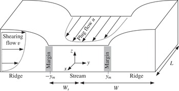To keep things simple, we assume a domain that is periodic in the $y$ -direction with sides at $y=\pm W$ , and has length $L$ along the $x$ -axis, where the latter is aligned with the main flow direction of the ice stream, see figure 1. Let a single ice stream occupy the region $-y_{m}<y<y_{m}$ , where $y_{m}(x,t)$ signifies the location of the ice stream margin. We assume that the latter can evolve in time: in fact, one of our main objectives is to improve on the model for the migration of ice stream margins developed in Schoof (Reference Schoof2012). Ice ridges occupy the remainder of the domain, where $y_{m}<|y|<W$ . To simplify matters further, we assume symmetry about $y=0$ .

Figure 1.

Geometry of the problem. We consider an ice stream whose principal direction of flow is along the $x$ -axis. The $y$ -direction is transverse to the flow, $z$ points vertically upwards. At its sides, the ice stream is bordered by slowly moving ice or ‘ice ridges’. The transition between ice stream and ice ridge is referred to here as the ice stream margin. It is located at $y=\pm y_{m}$ . The ice ridges are symmetrical about $y=\pm W$ .

Different boundary conditions apply under the ice stream and ice ridge. At the base of the ice stream, $|y|<y_{m}$ , $z=0$ , we assume that the direction of the tangential component of traction is given by the sliding velocity and its magnitude by a friction law,

where we assume $\boldsymbol{u}\neq \mathbf{0}$ . Here, ${\it\tau}_{b}$ is the magnitude of basal friction, which we assume to be given through a friction law as a function of the sliding speed $|\boldsymbol{u}|$ and possibly of other variables such as effective pressure $N$ (this being the difference between normal stress at the bed and water pressure in the bed, see e.g. Iken & Bindschadler Reference Iken and Bindschadler1986; Fowler Reference Fowler1987; Engelhardt & Kamb Reference Engelhardt and Kamb1997; Iverson et al. Reference Iverson, Baker, LeB Hooke, Hanson and Jansson1999; Kamb Reference Kamb, Alley and Bindschadler2001; Schoof Reference Schoof2005; Gagliardini et al. Reference Gagliardini, Cohen, Råback and Zwinger2007). We do not specify a particular friction law at this point, but will instead later assume that ${\it\tau}_{b}$ remains low enough everywhere in the ice stream to facilitate rapid sliding. Finally, $\hat{\boldsymbol{n}}$ is the inward- (or upward-) pointing unit vector, $\hat{\boldsymbol{n}}=(0,0,1)$ for a flat bed. In addition, we assume no basal melting or accretion of ice, so that

At the base of the ice ridges we assume that there is no slip,

for $|y|>y_{m}$ , $z=0$ . The abrupt switch from slip to no slip is known to lead to stress singularities (Hutter & Olunloyo Reference Hutter and Olunloyo1980; Barcilon & MacAyeal Reference Barcilon and MacAyeal1993; Schoof Reference Schoof2004; Moore, Iverson & Cohen Reference Moore, Iverson and Cohen2010), which can be alleviated if there is residual sliding even where the bed is frozen (Fowler Reference Fowler1986; Cuffey et al. Reference Cuffey, Conway, Hallet, Gades and Raymond1999; Schoof Reference Schoof2004). In keeping with making the simplest possible assumption, we retain the no-slip boundary condition (2.10) and address the regularizing effect of having limited slip at the bed of the ice ridge in a separate paper (Haseloff, Schoof & Gagliardini, in preparation).

We associate the switch from no slip to slip with temperature at the bed attaining the melting point. Consequently we need to solve for temperature $T$ . Within the ice, $0<z<s(x,y,t)$ , heat is both advected and conducted, and produced through strain heating, while in the bed, $z<0$ , there is only conduction:

Here, $c$ and $c_{bed}$ are the specific heat capacities of ice and bed, respectively, ${\it\rho}_{bed}$ is the density of the bed, and $k$ and $k_{bed}$ are the thermal conductivities of ice and bed.

We assume a constant temperature $T_{0}$ at the surface $z=s(x,y,t)$ and a constant incoming geothermal heat flux $q_{geo}$ at large depths below the bed:

At the ice–bed interface, we again have to distinguish between ice stream and ridge. At the base of the ice stream, the bed is at the melting point, while at the base of the ice ridge, temperature is below the melting point and the normal component of the heat flux is continuous:

Below, we non-dimensionalize the model in three different ways, appropriate to three distinct regions: the rapidly sliding ice stream, the slowly flowing ice ridge, and a narrow boundary layer that couples those regions together. This is in each case the basis for a simplified, leading-order model for ice flow and heat transport in each region. In the ridge and stream regions, these leading-order models are standard thin-film models, while in the boundary layer, we are primarily able to simplify the shape of the domain and boundary conditions, and to decouple partially the description of axial flow parallel to the ice stream in the boundary layer from transverse flow of ice across the boundary layer.

The scale applied to each variable is indicated by a square bracket with a subscript denoting the region under consideration. For example, $[u]_{r}$ is the scale for the velocity component $u$ in the ice ridge, which we then non-dimensionalize as $u=[u]_{r}u_{r}$ unless otherwise indicated, so that $u_{r}$ is then a dimensionless velocity in the ice ridge. Similarly, $[u]_{s}$ is the scale for the same velocity component in the ice stream, with $u_{s}$ the corresponding dimensionless velocity in the ice stream, while $[u]_{BL}$ is the scale in the boundary layer. 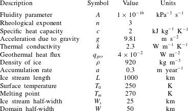To reduce the number of subscripts that ultimately appear, we use capital letters to denote dimensionless variables in the boundary layer, so $u=[u]_{BL}U$ in the boundary layer. Where we deviate from this convention, we explicitly specify the definition of the relevant dimensionless variable. Typical values of parameters and the characteristic scales which we use to guide our analysis are given in table 1.

Table 1.

Parameter values and characteristic scales.

Our approach is somewhat non-standard for what is ultimately an exercise in matched asymptotic expansions: rather than non-dimensionalizing the model once for one of the three regions identified and then rescaling the dimensionless model for the other two, we develop explicit scales for all variables in all three regions. This requires somewhat careful bookkeeping when we come to match asymptotically, but we have found our approach easier to motivate physically, and less confusing to present.

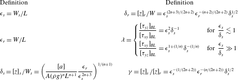
In particular, we find that a number of small parameters describing various geometrical aspect ratios arise naturally in the non-dimensionalization of ice ridge and ice stream flow. These are denoted by ${\it\epsilon}_{s}$ , ${\it\epsilon}_{r}$ for the width-to-length ratios of stream and ridge, and ${\it\delta}_{s}$ , ${\it\delta}_{r}$ for the respective thickness-to-width ratios. All are assumed to be small, which allows us to develop thin-film models for ice ridges and ice streams. However, although they appear naturally when non-dimensionalizing the Stokes equations for ice ridge and ice stream, they are not all mutually independent, which is where the careful bookkeeping becomes relevant (see table 2 for a summary). In addition, we obtain a fifth aspect ratio ${\it\lambda}$ (also not independent of the remaining aspect ratios) that gives a measure of ice surface slope in the boundary layer. Our leading-order model for the boundary layer is based on expanding in this additional aspect ratio ${\it\lambda}$ , which must also be small.

Table 2.

Aspect ratios used in the matched asymptotic expansions. The three ratios on the left, ${\it\epsilon}_{s}$ , ${\it\epsilon}_{r}$ and ${\it\delta}_{s}$ , can be chosen independently, in which case the remaining three ratios ${\it\delta}_{r}$ , ${\it\lambda}$ and ${\it\gamma}$ can be expressed as indicated. Our asymptotic expansions assume not only that ${\it\epsilon}_{s}\ll 1$ , ${\it\epsilon}_{r}\ll 1$ , ${\it\delta}_{s}\ll 1$ but also that ${\it\delta}_{r}\ll 1$ , ${\it\lambda}\ll 1$ as well as ${\it\gamma}\lesssim 1$ . This imposes additional constraints on the ratios ${\it\epsilon}_{s}$ , ${\it\epsilon}_{r}$ and ${\it\delta}_{s}$ in the form ${\it\delta}_{s}\ll {\it\epsilon}_{s}^{-(2n+3)/(n+1)}{\it\epsilon}_{r}^{(n+2)/(n+1)}$ , ${\it\delta}_{s}\lesssim {\it\epsilon}_{s}^{1/(n+1)}{\it\epsilon}_{r}^{n/(n+1)}$ , and either ${\it\epsilon}_{s}\lesssim {\it\delta}_{s}$ or ${\it\epsilon}_{s}^{1+1/n}\ll {\it\delta}_{s}\ll {\it\epsilon}_{s}$ . It is easy to see that such a parameter regime is possible.

3. Ice stream

The fast surface velocities of ice streams that are not confined to deep bedrock troughs (which we have already excluded by assuming a flat bed) can generally only be explained by rapid sliding at the bed, with comparatively little shearing across the thickness of the ice (e.g. Engelhardt & Kamb Reference Engelhardt and Kamb1998). Such ice streams flow as plug flows, and appropriate leading-order models of ice streams as rapidly sliding thin-film Stokes flows have been derived by e.g. Muszynski & Birchfield (Reference Muszynski and Birchfield1987) and MacAyeal (Reference MacAyeal1989). We follow these earlier authors, but additionally take the lateral confinement of the ice stream and its coupling with the surrounding ice ridge into account.

Our key assumptions are therefore that the ice stream has not only a small thickness-to-width (or vertical) aspect ratio, but also a small width-to-length (or plan view) aspect ratio, as is typically the case of a narrow and long ice stream. Later, we add four further assumptions: that the ice ridge likewise has small vertical and plan view aspect ratios, that the surface slope in the ice ridge is angled primarily towards the ice stream, and that the ratio of deviatoric to hydrostatic stresses in the boundary layer is small. The latter ensures that surface slopes remain small not only in the ridge and stream, but also in the shear margin. All of these basic assumptions are satisfied in practice by ice streams in West Antarctica.

We will show as we develop our leading-order model that these assumptions can be cast as constraints on just three independent dimensionless groups. The first is the plan aspect ratio of the ice stream, which we assume to be known (for instance, from the initial plan shape of the ice stream). If the stream has length $[x]_{s}=L$ and half-width $[y]_{s}=W_{s}$ , we assume that the plan view aspect ratio

is small. (Recall that the subscripted notation used here for scales and later for dimensionless variables is summarized at the end of § 2 above.) With $L\approx 1000~\text{km}$ and $W_{s}\approx 25~\text{km}$ , we have ${\it\epsilon}_{s}\approx 0.025$ . An analogous (but independent) plan aspect ratio for the domain as a whole can be defined as

With a spacing between neighbouring ice streams (and hence a domain width $2W$ ) of 100 km, ${\it\epsilon}_{r}\approx 0.05$ , and we will treat ${\it\epsilon}_{r}$ as small; naturally, as the ice stream cannot be wider than the domain, we always have ${\it\epsilon}_{s}<{\it\epsilon}_{r}$ .

The third independent dimensionless group is the vertical aspect ratio of the ice stream, which requires us to define a thickness scale $[z]_{s}$ . In addition to scales $L$ and $W_{s}$ , we assume that an accumulation rate scale $[a]$ is given, as are the material parameters $A$ , $n$ , ${\it\rho}$ and acceleration due to gravity $g$ . As we will see, it is possible to derive from these the appropriate scales for velocities, stresses and ice thickness.

We assume that pressure scales with its hydrostatic magnitude $[p]_{s}={\it\rho}g[z]_{s}$ . A balance between the longitudinal pressure gradient and lateral as well as vertical shear stresses yields $[{\it\tau}_{xy}]_{s}/W_{s}=[{\it\tau}_{xz}]_{s}/[z]_{s}=[p]_{s}/L$ , while balancing terms in the velocity divergence gives $[u]_{s}/L=[v]_{s}/W_{s}=[w]_{s}/[z]_{s}$ . Assuming flow dominated by lateral shearing, we put $[u]_{s}/W_{s}=A[{\it\tau}_{xy}]_{s}^{n}$ , while the normal stress components scale as $A[{\it\tau}_{xy}]^{n-1}[{\it\tau}_{xx}]_{s}=[u]_{s}/L$ , $A[{\it\tau}_{xy}]_{s}^{n-1}[{\it\tau}_{yy}]_{s}=[v]_{s}/W_{s}$ and $A[{\it\tau}_{xy}]_{s}^{n-1}[{\it\tau}_{zz}]_{s}=[w]_{s}/[z]_{s}$ . The vertical shear stress associated with transverse flow balances extensional stresses in that region, leading to $[{\it\tau}_{yz}]=[z]_{s}[{\it\tau}_{yy}]_{s}/W_{s}$ . The basal shear stress ${\it\tau}_{b}$ is assumed to scale as the vertical shear stress, $[{\it\tau}_{b}]_{s}=[{\it\tau}_{xz}]_{s}$ . Ice discharge through the width of the ice stream scales as $[u]_{s}[z]_{s}W_{s}$ , which we assume to balance net accumulation over the domain, $[u]_{s}[z]_{s}W_{s}=[a]WL$ . Lastly, as a temperature scale, we naturally choose $[T]=T_{m}-T_{0}$ , and pick the advective time scale $[t]=L/[u]_{s}$ . We omit the subscript $s$ on the latter two as the same scales for temperature and time apply to all three regions.

From the balances above, we can compute the scale for ice thickness in the ice stream as

from which we can define

where ${\it\delta}_{s}$ is independent of ${\it\epsilon}_{s}$ and ${\it\epsilon}_{r}$ ; $[z]_{s}$ defined in this way is the scale for ice thickness that emerges from requiring that discharge in the ice stream balances accumulation over the domain. If the assumptions stated in the previous paragraph about how different scales balance are correct, then the scale height $[z]_{s}$ should be comparable with the measured thickness of real ice streams; this is indeed the case. With the typical parameter values given in table 1, we find $[z]_{s}\approx 900~\text{m}$ and ${\it\delta}_{s}\approx 0.04$ . It is the fact that ${\it\delta}_{s}$ is small that allows us to develop a thin-film model for the ice stream.

The remaining scales for the ice stream flow problem can be expressed as

In addition to the aspect ratios ${\it\epsilon}_{s}$ , ${\it\epsilon}_{r}$ and ${\it\delta}_{s}$ , we obtain the following independent dimensionless groups that only appear in the heat flow component of our model:

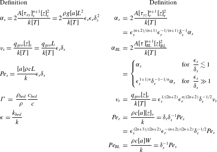
These are, respectively, a Péclet number for the ice stream, a dimensionless shear heating rate, a dimensionless geothermal heat flux, and two purely material ratios of heat capacities and thermal conductivities that we will treat as being $O(1)$ constants. With the parameter values in table 1, we get $\mathit{Pe}_{s}\approx 14$ , ${\it\alpha}_{s}\approx 6$ and ${\it\nu}_{s}\approx 0.8$ . Note that a summary of all aspect ratios used in this paper may be found in table 2, while all other dimensionless groups used are listed in table 3. In what follows, we assume that the three aspect ratios ${\it\epsilon}_{s}$ , ${\it\epsilon}_{r}$ and ${\it\delta}_{s}$ are all small, while we treat the thermal parameters $\mathit{Pe}_{s}$ , ${\it\alpha}_{s}$ and ${\it\nu}_{s}$ as potentially $O(1)$ for now.

Table 3.

Dimensionless groups. ${\it\alpha}_{s}$ , $\mathit{Pe}_{s}$ , ${\it\nu}_{s}$ , ${\it\Gamma}$ and ${\it\kappa}$ are independent dimensionless groups in the model along with ${\it\epsilon}_{s}$ , ${\it\epsilon}_{r}$ and ${\it\delta}_{s}$ . The remaining model parameters can be expressed through these, as indicated.

4. Ice ridge

We assume that the ice is frozen to the bed and that there is no slip under the ice ridges. Ice therefore moves by vertical shear alone with surface velocities that are much slower than in the adjacent ice stream. We also assume that ice is thicker in the ice ridge than in the ice stream and the resulting gradient in surface elevation leads to a gravity-driven inflow of ice into the ice stream.

By symmetry, we restrict ourselves to the ice ridge on the left (looking upstream, see figure 1), for which $-W<y<-y_{m}$ . Consequently, we rescale the lateral coordinate as $y=[y]_{r}y_{r}-W$ with $[y]_{r}=W$ . The length scale $[x]_{r}=[x]_{s}=L$ is the same as for the ice stream, and the relevant plan aspect ratio is ${\it\epsilon}_{r}=W/L$ as defined before. In order to arrive at a thin-film model, we also need to define a small vertical aspect ratio ${\it\delta}_{r}=[z]_{r}/W$ , which requires us to identify a thickness scale $[z]_{r}$ for the ice ridge. There is no a priori reason why this should be the same as for the ice stream, and we go again through the same exercise of finding the relevant balance of scales for the ice ridge.

If the dominant motion in the ice ridge is through vertical shear, then vertical shear stress balances the driving pressure gradient, so $[{\it\tau}_{xz}]_{r}/[z]_{r}=[p]_{r}/L$ and $[{\it\tau}_{yz}]_{r}/[z]_{r}=[p]_{r}/W$ , where $[p_{r}]={\it\rho}g[z]_{r}$ . Flow is dominantly towards the ice stream, so $[v]_{r}/[z]_{r}=A[{\it\tau}_{yz}]_{r}^{n}$ while $[u]_{r}/[z]_{r}=A[{\it\tau}_{yz}]_{r}^{n-1}[{\it\tau}_{xz}]_{r}$ . Mass conservation, (2.4), suggests $[v]_{r}/W=[w]_{r}/[z]_{r}$ with $[w]_{r}=[a]$ where $[a]$ is the scale of the surface accumulation. Scales for the remaining stress components are $[u]_{r}/[x]_{r}=A[{\it\tau}_{yz}]_{r}^{n-1}[{\it\tau}_{xx}]_{r}$ , $[v]_{r}/[y]_{r}=A[{\it\tau}_{yz}]_{r}^{n-1}[{\it\tau}_{yy}]_{r}$ , $[w]_{r}/[z]_{r}=A[{\it\tau}_{yz}]_{r}^{n-1}[{\it\tau}_{zz}]_{r}$ , and $[u]_{r}/[y]_{r}=A[{\it\tau}_{yz}]_{r}^{n-1}[{\it\tau}_{xy}]_{r}$ .

The balances above define a new thickness scale through

which gives us the required fourth aspect ratio ${\it\delta}_{r}=[z]_{r}/W$ , which we assume to be small. Note, however, that ${\it\delta}_{r}$ is not independent of the previously defined parameters ${\it\epsilon}_{s}$ , ${\it\epsilon}_{r}$ , ${\it\delta}_{s}$ , but can be expressed as

We are therefore not only assuming that ${\it\epsilon}_{s}$ , ${\it\epsilon}_{r}$ , ${\it\delta}_{s}$ are small, but also that

Such a parameter regime clearly exists, and applies to real ice ridges, which have low aspect ratios: with the parameter estimates in table 1 we get ${\it\delta}_{r}=0.02$ .

With ${\it\delta}_{r}$ defined, the remaining scales can now be expressed as

while scales for time and temperature are the same as those for the ice stream.

From these scales, we can also form new versions of the Péclet number, shear heating rate and geothermal heat flux as

As with ${\it\delta}_{r}$ , these are, however, not independent of their equivalents in the ice stream, but related to the latter through

Note that the ratio of the Péclet numbers in the ice ridge and ice stream equals the ratio of the vertical aspect ratios in the two regions, and the ratio of the scaled geothermal heat fluxes depends only on the ratio between the thickness scales in the two regions. With the parameter estimates in table 1 we obtain $[z]_{s}\approx 900~\text{m}$ and $[z]_{r}\approx 970~\text{m}$ , and therefore calculate values of $\mathit{Pe}_{r}$ and ${\it\nu}_{r}$ that are similar to those in the ice stream: we get $\mathit{Pe}_{r}\approx 7$ and ${\it\nu}_{r}\approx 0.8$ , as well as ${\it\alpha}_{r}\approx 4$ . As before, we retain these for now as being potentially $O(1)$ .

5. The margin boundary layer

In the last two sections we have derived equations that describe the evolution of an ice stream, (3.15) and (3.18a–c ), and of an ice ridge adjacent to it, (4.16) and (4.17). The ice stream moves as a plug flow through a ‘channel’ formed by the ice ridges, where ice moves through vertical shear towards the ice stream. At present we can only speculate about the appropriate coupling between the two models. For instance, we might expect the inflow $q_{in}$ in (3.18c ) to be related to the ice ridge flux $q_{r}$ in (4.17) at the margin. However, due to the distinct nature of the velocity fields in the stream and ridge – one is a plug flow, the other a shearing flow – coupling is not trivial and a boundary layer is required. Similar boundary layers are encountered in other settings in ice sheet dynamics, for instance around the grounding line of marine ice sheets (Chugunov & Wilchinsky Reference Chugunov and Wilchinsky1996).

The boundary layer here is located between the ice stream and the ice ridge in the region around $y=\pm y_{m}(x,t)$ , which we refer to as the ice stream margin. As with the ice ridge, we focus on the margin to the left of the ice stream near $y=-y_{m}$ . Within the boundary layer a spatially rapid transition from the Poiseuille-type flow in the ice ridge to the plug flow in the ice stream has to take place. The boundary layer cannot be shallow – otherwise we would expect one kind of thin-film approximation or the other to hold – and to account for continuity of the surface with the adjacent stream, we choose the scales $[y]_{BL}=[z]_{BL}=[z]_{s}$ . We rescale the lateral coordinate $y=[y]_{BL}Y-[y]_{s}y_{M}(x_{s},t)$ , so that the boundary layer coordinate is centred around the transition between a frozen bed and an unfrozen temperate bed that occurs in the left-hand margin at $y_{s}=-y_{M}$ , $Y=0$ .

To account for mass flux from the ridge through the margin into the ice stream, we put $[v]_{BL}[z]_{BL}=[v]_{s}[z]_{s}=[a]W$ , or $[v]_{BL}=[v]_{s}$ , while mass balance requires $[v]_{BL}=[w]_{BL}$ . The ice stream imposes a lateral shear stress on the boundary layer, which must be balanced by vertical shear stresses in the boundary layer and leads us to put $[{\it\tau}_{xz}]_{BL}=[{\it\tau}_{xy}]_{BL}=[{\it\tau}_{xy}]_{s}$ .

Shearing due to transverse flow in the boundary layer leads to $[v]_{BL}/[z]_{BL}=A[{\it\tau}]_{BL}^{n-1}[{\it\tau}_{yz}]_{BL}$ . There are now two possible cases: the second stress invariant ${\it\tau}$ in the boundary layer can be dominated either by shear stresses due to transverse flow, so that $[{\it\tau}]_{BL}=[{\it\tau}_{yz}]_{BL}$ , or by lateral shear stresses, so that $[{\it\tau}]_{BL}=[{\it\tau}_{xy}]_{BL}$ . In the first case, the scaled stress invariant becomes $\mathscr{T}=(\mathscr{T}_{xy}^{2}+\mathscr{T}_{xz}^{2}+({\it\epsilon}_{s}/{\it\delta}_{s})^{2}\mathscr{T}_{yz}^{2}+\cdots \,)^{1/2}$ , where $\mathscr{T}_{ij}$ denotes dimensionless stress components. It is clear that this scaling is only appropriate for ${\it\epsilon}_{s}/{\it\delta}_{s}\lesssim 1$ . Similarly, the second version is only appropriate for ${\it\epsilon}_{s}/{\it\delta}_{s}\gtrsim 1$ , but to be definite when ${\it\epsilon}_{s}\sim {\it\delta}_{s}$ , we define $[{\it\tau}]_{BL}=[{\it\tau}_{yz}]_{BL}$ only when ${\it\epsilon}_{s}/{\it\delta}_{s}\gg 1$ , and put $[{\it\tau}]_{BL}=[{\it\tau}_{xy}]_{BL}$ otherwise.

The scale of the downstream velocity is defined through $[u]_{BL}/[z]_{BL}=A[{\it\tau}]_{BL}^{n-1}[{\it\tau}_{xy}]_{BL}$ , and the normal components of the stress are determined through $[u]_{BL}/[x]_{BL}=A[{\it\tau}]_{BL}^{n-1}[{\it\tau}_{xx}]_{BL}$ , $[v]_{BL}/[y]_{BL}=A[{\it\tau}]_{BL}^{n-1}[{\it\tau}_{yy}]_{BL}$ and $[w]_{BL}/[z]_{BL}=A[{\it\tau}]_{BL}^{n-1}[{\it\tau}_{zz}]_{BL}$ . We assume that the basal drag in the unfrozen part of the margin is comparable with the basal drag in the ice stream, which for instance would be appropriate if the bed of the margin was hydraulically well connected to the ice stream bed, and we therefore put $[{\it\tau}_{b}]_{BL}=[{\it\tau}_{b}]_{s}$ .

The leading-order models for the two cases in ${\it\epsilon}_{s}/{\it\delta}_{s}$ identified above (which differ in terms of which stresses dominate the stress invariant and therefore ice viscosity and heat dissipation in the boundary layer) are very similar and we can treat them both succinctly by defining a parameter ${\it\lambda}$ through

${\it\lambda}$ turns out to be the ratio of deviatoric normal stresses to hydrostatic pressure in the boundary layer. We will assume below that ${\it\lambda}\ll 1$ , which ensures that the surface slope in the boundary layer remains small and we can treat the boundary layer at zeroth order as occupying a fixed domain with a flat upper surface. We always have ${\it\lambda}\ll 1$ when ${\it\epsilon}_{s}/{\it\delta}_{s}\lesssim 1$ , while for ${\it\epsilon}_{s}/{\it\delta}_{s}\gg 1$ , we require an additional constraint

This is in addition to the constraint ${\it\epsilon}_{s}^{(2n+3)/(n+2)}{\it\delta}_{s}^{(n+1)/(n+2)}\ll {\it\epsilon}_{r}\ll 1$ from (4.3). A compilation of all the constraints that we impose on the independent parameters ${\it\epsilon}_{s}$ , ${\it\epsilon}_{r}$ and ${\it\delta}_{s}$ is given in the caption to table 2.

From the balances identified above, the relevant scales for the boundary layer can now be expressed as

while the scales for time and temperature are again the same as those for the ice stream itself.

In addition to the parameter ${\it\lambda}$ defined above, we obtain new versions of the Péclet number and dimensionless shear rate, $\mathit{Pe}_{BL}={\it\rho}c[a]W/k$ and ${\it\alpha}_{BL}=2A[{\it\tau}]_{BL}^{n+1}[z]_{BL}^{2}/(k[T]_{BL})$ . As with $\mathit{Pe}_{r}$ and ${\it\alpha}_{r}$ , $\mathit{Pe}_{BL}$ and ${\it\alpha}_{BL}$ are not independent of $\mathit{Pe}_{s}$ , ${\it\alpha}_{s}$ , ${\it\epsilon}_{s}$ , ${\it\epsilon}_{r}$ and ${\it\delta}_{s}$ , but can be written in the form

With the typical values in table 1, we obtain $\mathit{Pe}_{BL}\approx 380$ and ${\it\alpha}_{BL}\approx 6$ .

6. Matching

The boundary layer solutions have to match the solutions in the outer regions, the ice stream and ridge. Even though we have motivated all our scales physically, the spatial coordinates and dependent variables used to describe the stream, ridge and boundary layer can be related purely through rescalings using the independent aspect ratios ${\it\epsilon}_{s}$ , ${\it\epsilon}_{r}$ , ${\it\delta}_{s}$ , and the derived dimensionless groups ${\it\delta}_{r}$ and ${\it\lambda}$ defined in terms of ${\it\epsilon}_{s}$ , ${\it\epsilon}_{r}$ and ${\it\delta}_{s}$ in (4.2) and (5.1), respectively. We list these rescalings here for completeness:

7. Solution of the boundary layer model

In terms of the mechanical and kinematic coupling between the ice stream and ice ridge flow models, the margin boundary layer turns out to be essentially passive. The ice ridge is coupled to the ice stream by having to match the ice stream surface height at the interface between the two, which becomes the relevant boundary condition for (4.16). Conversely, the ice stream velocity problem (3.15) has to satisfy a zero velocity boundary condition at the ice stream margins $y=\pm y_{m}$ , while the stream couples to the ridge through continuity of flux, setting $q_{in}=2s_{s}\partial y_{M}/\partial t+2q_{M}$ in (4.17). We were able to obtain these intuitive results by matching stream to ridge across the boundary layer without actually having to solve the boundary layer equations.

By contrast, the boundary layer holds the key to computing the margin migration rate $\partial y_{M}/\partial t$ . The problem for temperature $T$ in the boundary layer (5.12), (5.13), (6.7) and (6.18) is nearly identical to the ice stream margin problem in Schoof (Reference Schoof2012), and the latter predicts a unique solution for the margin migration rate as a function of various forcing parameters. The boundary layer model here generalizes Schoof’s version through the addition of an advection term that accounts for transverse flow through the margin. Schoof’s model is restricted to a widening ice stream with $\partial y_{M}/\partial t>0$ (see, however, the appendix to Schoof’s paper for a discussion of the opposite case). For a widening stream, it is necessary to add a constraint on heat fluxes on the ice stream side of the temperate–frozen transition at $Y=0$ :

If this condition was violated, then as the ice stream widens the newly unfrozen bed would be subjected to net heat loss. At this point the bed should not yet contain any liquid water to freeze and would not remain unfrozen in contradiction to our assumption that the ice stream is widening. We adopt the same assumptions, adding the constraint (7.1) to the temperature constraint (5.13e ) already in place on the temperate side of the cold–temperate transition at $Y=0$ .

We make one further expedient simplification here, which is not truly justified by our scale estimates: we treat the Péclet number $\mathit{Pe}_{BL}$ as an $O(1)$ quantity. The realistic limit of large Péclet numbers can be dealt with in the framework we have developed, but this is somewhat involved and therefore beyond the scope of this paper. Our aim is to demonstrate how transverse flow affects the lateral migration rates computed by Schoof (Reference Schoof2012), for which treating $\mathit{Pe}_{BL}$ as $O(1)$ provides a useful first step. Similarly, we treat ${\it\alpha}_{BL}$ as $O(1)$ .

In addition, we assume that ${\it\epsilon}_{s}/{\it\delta}_{s}\ll 1$ in the boundary layer model, which corresponds to the case of lateral shear stresses dominating over stresses generated by transverse inflow across the margin (see (5.6)). Even though our scale estimates suggest that ${\it\epsilon}_{s}$ is not much smaller than ${\it\delta}_{s}$ , a dominant lateral shear stress is actually the most realistic scenario for a real ice stream: the lateral shear stresses predicted by our scale estimates are somewhat smaller than those inferred from direct observations.

The limit of small ${\it\epsilon}_{s}/{\it\delta}_{s}$ in principle should let us simplify viscosity and heat production rates as

However, in the case of the viscosity, omitting the $O({\it\epsilon}_{s}^{2}/{\it\delta}_{s}^{2})$ terms due to lateral inflow is problematic as the derivatives of $U^{(0)}$ vanish in the far field as $Y\rightarrow -\infty$ . With $n>1$ , this leads to an infinite viscosity. In principle this can be fixed through the introduction of yet another (rather trivial and passive) boundary layer in which all the velocity gradients are of similar size, but it is in practice (especially numerically) simpler to retain the additional velocity gradients due to lateral inflow in the viscosity.

To close the temperature problem, we also assume that the temperature field in the matching region with the ridge can be treated as being piecewise linear, with the temperature gradient given by the geothermal heat flux:

It turns out that this is formally the correct temperature solution for the ridge in the parameter regime we have just defined: from $\mathit{Pe}_{r}={\it\delta}_{r}\mathit{Pe}_{BL}$ (see table 3), the ridge Péclet number is small if $\mathit{Pe}_{BL}$ is of $O(1)$ , while the ridge shear heating parameter ${\it\alpha}_{r}$ is also small: with ${\it\alpha}_{r}=({\it\epsilon}_{s}/{\it\delta}_{s})({\it\epsilon}_{s}/{\it\epsilon}_{r})^{1/(n+1)}{\it\alpha}_{BL}$ as well as ${\it\epsilon}_{s}/{\it\epsilon}_{r}=W_{s}/W<1$ and ${\it\epsilon}_{s}/{\it\delta}_{s}\ll 1$ , it follows that ${\it\alpha}_{r}\ll {\it\alpha}_{BL}=O(1)$ . With small $\mathit{Pe}_{r}$ and ${\it\alpha}_{r}$ , we obtain a linear temperature profile $T_{r}={\it\nu}_{r}(s_{r}-z_{r})-1$ as solution of (4.13a ). This is of course contrived, as $\mathit{Pe}_{BL}$ and ${\it\alpha}_{BL}$ should not be treated as $O(1)$ , and less trivial far-field temperature fields are possible in real ice sheets. As mentioned, these more complicated cases will be dealt with separately, and (7.3) for now provides a convenient, self-consistent closure to the boundary layer heat equation.

8. Discussion and conclusions

In this paper, we have developed two closely related models, both summarized in § 7.1. The first is a mechanical boundary layer description of the junction between the slow shearing flow of an ice ridge and a rapidly sliding, lateral-stress-dominated plug flow of an ice stream. The second is a model for the migration of that junction as a result of heat dissipation in the ice stream margin. Both models are based on the assumption that the margin of an ice stream coincides with a switch from a well-lubricated bed at the melting point, where rapid sliding is possible, to a frozen bed where no slip occurs. This does not preclude the possibility that the margins of some ice streams could be fixed by other means, for instance abrupt changes in subglacial water pressure (Kyrke-Smith et al. Reference Kyrke-Smith, Katz and Fowler2014) or more exotic multiple-valued sliding laws (Sayag & Tziperman Reference Sayag and Tziperman2011).

Our mechanical boundary layer consists of a weakly coupled version of the model for lateral-stress-driven shearing in an idealized ice stream shear margin in Schoof (Reference Schoof2004, Reference Schoof2012) and the model for ice flow across the equally idealized upstream onset of an ice stream in Barcilon & MacAyeal (Reference Barcilon and MacAyeal1993), although in our case the geometry is somewhat different from that in Barcilon and MacAyeal’s work (and therefore so are the far-field boundary conditions, in particular on the surface perturbation $S^{(1)}$ ). The weak coupling between the two flow problems in the boundary layer comes about through the strain-rate-dependent viscosity we have assumed, while the models in Schoof (Reference Schoof2004, Reference Schoof2012) and Barcilon & MacAyeal (Reference Barcilon and MacAyeal1993) were formulated for the Newtonian case. The margin migration model in turn is a generalized form of that in Schoof (Reference Schoof2012), which we re-derive from first principles in the process of constructing the boundary layer model, and to which we add lateral advection of heat due to inflow of ice from the ridge into the stream.

The mechanical boundary layer model provides a self-consistent way of deriving the appropriate jump conditions between ridge and stream at the ice stream margin, which turn out to be the rather intuitive continuity of ice flux and ice thickness, as well as zero axial ice stream velocity at the margin. This generalizes the ad hoc formulation of jump conditions in prior work that couples leading-order ridge and stream models (e.g. Hulbe & MacAyeal Reference Hulbe and MacAyeal1999; Ritz, Rommelaere & Dumas Reference Ritz, Rommelaere and Dumas2001). There is, however, a caveat here: we have explicitly required the ice stream and ice ridge to be narrow as well as shallow in developing the boundary layer model, while the papers cited above do not. The main difference this leads to is that the velocity field solved for in Hulbe & MacAyeal (Reference Hulbe and MacAyeal1999) and Ritz et al. (Reference Ritz, Rommelaere and Dumas2001) is two-dimensional, while ours consists only of the axial velocity $u_{s}$ in (3.15), with the cross-stream velocity field $v_{s}$ a higher-order correction. A two-dimensional extension to the elliptic problem (3.15) naturally requires a second boundary condition. One might assume that continuity of depth-integrated normal velocity across the stream margin fixes the problem.

Making that assumption, however, turns out to be non-trivial: the narrowness of our ice stream is crucial to ensuring that normal stresses at the ice stream margin remain small relative to hydrostatic (or ‘cryostatic’) stresses, which is fundamental to our boundary layer model. Technically, it allows a parameter regime in which the relevant stress ratio ${\it\lambda}$ defined in § 5 is small. For ice streams that are not narrow, normal stress will typically be comparable to cryostatic stresses, and the stress balance becomes similar to that at a marine ice sheet grounding line in which the grounded sheet does not slide (Chugunov & Wilchinsky Reference Chugunov and Wilchinsky1996; Nowicki & Wingham Reference Nowicki and Wingham2008; Fowler Reference Fowler2011, chapter 10.2): slopes in the boundary layer will be $O(1)$ , and the ice stream will be much thinner than the ice ridge, so continuity of ice thickness need no longer be the appropriate jump condition, and the boundary layer problem becomes harder to solve.

The extension of our model to the migration of ice stream margins is based on solving the heat equation in the boundary layer, requiring the migration velocity to be rapid enough so that the part of the bed that is subject to a no-slip boundary condition does not reach the melting point, while also requiring it to be slow enough not to cause freezing on the part of the bed where sliding does occur. As in Schoof (Reference Schoof2012), we find that there is a single migration velocity that satisfies both of these constraints for any given set of forcing parameters, at least within what appears to be numerical error. Our boundary layer model puts Schoof’s work on a more solid foundation, and further generalizes it to take account of heat transport due to lateral inflow of cold ice from the ice ridges. We find that this inflow significantly suppresses temperatures in the margin and reduces migration velocities.

There are several complications to the margin migration model that we will address in separate papers. In our model formulation, we have treated the Péclet number in the margin as being $O(1)$ , whereas in reality it should be large, indicating that diffusion is ineffective over most of the boundary layer domain: this is equivalent to the contention in Fowler (Reference Fowler2013) that Schoof’s margin migration model requires a pseudo-steady temperature field to be established in the margin due to diffusion alone, which requires very long time scales. In a separate paper (Haseloff et al., in preparation), we will show how the boundary layer model can be adapted to the case of large Péclet numbers. In addition, we have assumed that there is an abrupt transition from slip to no slip, which introduces a questionable singularity into the stress and shear heating fields, which partly explains the need for a very high mesh resolution in our numerical solutions, and can be alleviated by permitting at least a small amount of sliding on the ‘frozen’ side of the margin. Similarly, the additional physics introduced by the formation of temperate ice (in which the temperature reaches the melting point within the domain, see e.g. Suckale et al. Reference Suckale, Platt, Perol and Rice2014) have also been ignored in this paper. We will address both of these complications in detail elsewhere. A further complication that we have omitted from this work is the temperature-dependence of ice viscosity: at its most extreme, this could lead to effectively shear-weakening behaviour of the near-marginal ice, when depth-averaged (Perol et al. Reference Perol, Rice, Platt and Suckale2015).

We conclude by noting that the need for a boundary layer description may not be obvious in view of the types of models that underpin modern numerical ice sheet simulations. Many of these have moved away from coupling leading-order, lubrication-type ‘shallow ice’ models for ridges to membrane-type ‘shallow stream’ models across ice stream margins, and employ a hybrid formulation using so-called ‘higher-order’ models that can be applied regardless of how fast the ice sheet slides (Pattyn Reference Pattyn2003; Bueler & Brown Reference Bueler and Brown2009; Cornford et al. Reference Cornford, Martin, Graves, Ranken, Le Brocq, Gladstone, Payne, Ng and Lipscomb2013; Kyrke-Smith et al. Reference Kyrke-Smith, Katz and Fowler2013). These are, however, still thin-film models that do not apply in regions where the velocity field changes by $O(1)$ over a single ice thickness (Schoof & Hindmarsh Reference Schoof and Hindmarsh2010), and therefore cannot be relied on to describe the physics of the stream–ridge boundary layer. Naturally, this restriction does not apply to models that either solve the Stokes equations in the entire domain (Gillet-Chaulet et al. Reference Gillet-Chaulet, Gagliardini, Seddik, Nodet, Durand, Ritz, Zwinger, Greve and Vaughan2012), or adaptively determine the location of localized high-shear zones in which the Stokes equations must be solved instead of a higher-order model (Seroussi et al. Reference Seroussi, Ben Dhia, Morlighem, Larour, Rignot and Aubry2012). However, while these approaches may handle the mechanical aspects of an ice stream shear margin adequately, it is still unlikely that they would be capable of solving our margin migration problem in practice: in order to reproduce known solutions to the margin migration problem, we found mesh resolutions around 10⁻⁶ times the ice thickness to be necessary near the transition from a frozen to a temperate bed. It is unlikely that such resolutions would be feasible even locally in large-scale ice sheet simulations, and a separate solution to the boundary layer problem seems more promising, computing margin migration velocity as a function of forcings imposed by ridge and stream.