1 Introduction
A novel super-large-scale particle image velocimetry (SLPIV) and visualization technique, which uses snowflakes as tracers, was recently developed by Hong et al. (Reference Hong, Toloui, Chamorro, Guala, Howard, Riley, Tucker and Sotiropoulos2014) for measuring the near-wake turbulent flow structures of utility-scale wind turbines. A field experiment using this technique was carried out on the Clipper Liberty C96 2.5 MW wind turbine at the EOLOS wind energy research field station (Hong et al.
Reference Hong, Toloui, Chamorro, Guala, Howard, Riley, Tucker and Sotiropoulos2014; Chamorro et al.
Reference Chamorro, Lee, Olsen, Milliren, Marr, Arndt and Sotiropoulos2015b
; Howard & Guala Reference Howard and Guala2016), University of Minnesota, from 2:00 am to 3:30 am on 22 February, 2013. The Clipper turbine has a rotor with diameter
 $D=96~\text{m}$
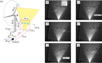
installed on a nacelle located 80 m above ground. The corresponding SLPIV set-up is shown in figure 1(a). The tip vortex patterns visualized in this experiment at different time instants, which are identified as voids in the snow generated by centrifugal forces ejecting snow particles out of vortex cores, are shown in figures 1(b) to 1(g). We usually expect round-like tip vortex patterns as visualized in many model-scale experiments (Hu, Yang & Sarkar Reference Hu, Yang and Sarkar2012; Sherry et al.
Reference Sherry, Nemes, Jacono, Blackburn and Sheridan2013; Zhang, Markfort & Porté-Agel Reference Zhang, Markfort and Porté-Agel2013; Chamorro et al.
Reference Chamorro, Hill, Neary, Gunawan, Arndt and Sotiropoulos2015a
). However, as seen in figure 1, vortex cores of complex shape were visualized resembling circular cores with attached elongated comet-like tails extending into the outer tip shear layer and inclined downwind. In addition to the pattern of a circular core with a single tail, which occurs most frequently in the visualization images, another pattern could also be identified resembling a core with two inclined tails like an inverted U shape (see figure 1
c). Different angles of inclination of these void patterns are observed ranging from approximately 25° to 45°. Moreover, we found patterns like those observed in figure 1 persist in all the images recorded during our field deployment.
(a) Set-up of SLPIV measurements adapted from Hong et al. (Reference Hong, Toloui, Chamorro, Guala, Howard, Riley, Tucker and Sotiropoulos2014). (b)–(g) Snow voids from snow visualization images at different time instants with time increment 1 s. The rotor period during the experiment is approximately 5 s. Circular voids with single and double tails are observed along the rotor tip shear layer. Vertical inboard vortex sheets are also visualized as lines of voids in the wake of the blades.

These unusual (for wind turbine tip vortex cores) patterns of snow voids seem to indicate complex coherent dynamics near the outer tip shear layer the origin and governing mechanisms of which could not be identified using the SLPIV data. In this work, we employ high-fidelity large-eddy simulation with the turbine rotor modelled as rotating actuator surfaces to simulate the flow fields in the turbine near wake in order to elucidate the dynamics underlying these complex tip vortex patterns and uncover the governing mechanisms.
2 Numerical methods
We carry out large-eddy simulation (LES) by solving numerically the spatially filtered, unsteady, three-dimensional, incompressible Navier–Stokes and continuity equations. The subgrid-scale stress tensor is modelled by the dynamic eddy-viscosity subgrid-scale model (Germano et al. Reference Germano, Piomelli, Moin and Cabot1991). The governing equations are discretized on a hybrid staggered/non-staggered grid using three-point central finite differencing and integrated in time via a second-order accurate fractional step method. An algebraic multigrid acceleration along with the GMRES solver are used to solve the pressure Poisson equation and a matrix-free Newton–Krylov method is used for the filtered momentum equation. The numerical method satisfies the discrete continuity equation to machine zero at each time step. The details of the methodology can be found in Kang et al. (Reference Kang, Lightbody, Hill and Sotiropoulos2011) and Yang et al. (Reference Yang, Sotiropoulos, Conzemius, Wachtler and Strong2015b ).
We employ an actuator surface approach to model the rotor blades. The actuator surface concept was originally proposed by Shen, Zhang & Sørensen (Reference Shen, Zhang and Sørensen2009) and allows for a better representation of the blade geometry than the standard actuator line approach. In the actuator surface approach, the forces imparted from the blade to the flow are distributed from the actuator surface formed by the airfoil chord instead of the actuator line (Sørensen & Shen Reference Sørensen and Shen2002; Yang et al.
Reference Yang, Sotiropoulos, Conzemius, Wachtler and Strong2015b
). The forces in the present actuator surface model are calculated based on a blade element approach instead from the pressure coefficient of the blades as in Shen et al. (Reference Shen, Zhang and Sørensen2009). To distribute the force from the blade to the flow and interpolate the velocity to the blade location, we employ the discrete delta function in the form of
 $\unicode[STIX]{x1D6FF}_{h}(\boldsymbol{x}-\boldsymbol{X})=(1/h^{3})\unicode[STIX]{x1D719}((x-X)/h)\unicode[STIX]{x1D719}((y-Y)/h)\unicode[STIX]{x1D719}((z-Z)/h)$
, where
 $\boldsymbol{x}$
,
 $\boldsymbol{X}$
are the coordinates of background grid and actuator surface grid, respectively,
 $\unicode[STIX]{x1D719}$
is the smoothed four-point cosine function proposed by Yang et al. (Reference Yang, Zhang, Li and He2009), with distribution width
 $5h$
. In immersed boundary methods
 $h$
is equal to the grid spacing. In the actuator-type simulations of wind turbines, however, the width of the force distribution essentially determines the size of the tip vortex. This implies that the vortex core will become smaller if a finer mesh is employed. Here the
 $h$
is selected such that it can mimic the size of the tip vortex core visualized by the SLPIV technique and satisfy the force conservation during the force distribution in the meantime. In the present case, the employed
 $h=D/80$
with the grid spacing near the turbine being equal to
 $D/160$
. This results in the width of the force distribution to be
 $0.0625D$
, which is consistent with the size of the snow voids measured in the field, i.e. approximately
 $0.042D$
–
 $0.073D$
(4–7 m). Validation of this actuator surface model in predicting the tip vortices is presented in appendix B.
3 Test cases and computational details
While SLPIV results are only available for the Clipper turbine, we will seek herein to systematically probe the dependence of the phenomena we uncover on turbine design, size and inflow conditions. For that, and in addition to the Clipper turbine, we also carry out simulations for two additional field-scale wind turbines: SWiFT and MEXICO turbines, and the model wind turbine of Lignarolo et al. (Reference Lignarolo, Ragni, Scarano, Ferreira and van Bussel2015). In this section we first describe briefly the details of various turbine designs we consider. Subsequently, we present the method we employ to generate inflow conditions and discuss various computational details.
3.1 Wind turbine designs
The four wind turbine designs we consider herein are: (i) the 2.5 MW Clipper turbine installed at the University of Minnesota EOLOS wind energy research field station, which has been described extensively in a number of previous publications (Hong et al. Reference Hong, Toloui, Chamorro, Guala, Howard, Riley, Tucker and Sotiropoulos2014; Yang et al. Reference Yang, Annoni, Seiler and Sotiropoulos2014a ; Chamorro et al. Reference Chamorro, Lee, Olsen, Milliren, Marr, Arndt and Sotiropoulos2015b ); (ii) a turbine design presented by Kelley, Maniaci & Resor (Reference Kelley, Maniaci and Resor2015) for the Scaled Wind Farm Technology (SWiFT) facility (Barone & White Reference Barone and White2011; Berg et al. Reference Berg, Bryant, LeBlanc, Maniaci, Naughton, Paquette, Resor, White and Kroeker2014; Kelley et al. Reference Kelley, Maniaci and Resor2015; Yang et al. Reference Yang, Boomsma, Barone and Sotiropoulos2014b , Reference Yang, Boomsma, Sotiropoulos, Kelley, Maniaci and Resor2015a ) developed by Sandia National Laboratories in Lubbock, TX, USA; (iii) the MEXICO wind turbine developed in the European collaborative MEXICO (Model Experiments in Controlled Conditions) project (Schepers & Snel Reference Schepers and Snel2007; Shen, Zhu & Sørensen Reference Shen, Zhu and Sørensen2012; Nilsson et al. Reference Nilsson, Shen, Sørensen, Breton and Ivanell2015); and (iv) the model wind turbine of Lignarolo et al. (Reference Lignarolo, Ragni, Krishnaswami, Chen, Ferreira and Van Bussel2014, Reference Lignarolo, Ragni, Scarano, Ferreira and van Bussel2015). The rotor diameters of the Clipper turbine, the SWiFT turbine, the Mexico turbine and the model wind turbine are 96 m, 27 m, 4.5 m and 0.6 m, respectively. The optimal tip speed ratios are approximately 8.3, 9, 6.7 and 6 for the Clipper turbine, the SWiFT turbine, the MEXICO turbine and the model wind turbine, respectively. More details about the employed turbines can be found in the papers cited above and are omitted herein.
3.2 Inflow conditions
For the SWiFT turbine, the MEXICO turbine and the model turbine cases, we only carry out simulations under the uniform inflow condition (Inflow 1).
For the Clipper turbine, however, we consider simulations both under uniform flow and varying turbulent inflow conditions. One of the turbulent inflow cases is designed to emulate as closely as possible the state of the atmosphere and approach flow when the SLPIV experiment was carried out in order to facilitate comparisons between simulations and field experiments. During the period of the SLPIV measurements, the wind blows from 54° (clockwise from North) at 2:00 am to 34° around 3:30 am on 22 February, 2013. The thermal stratification was weakly stable. The measured velocity time series from 3:00 to 3:30 am on that day from the sonic anemometer installed at
 $z=30~\text{ m}$
on the meteorological tower of the EOLOS facility are employed to calculate the turbulence intensity characterizing the atmospheric turbulence around the rotor bottom tip. During that time period, the incoming wind speed
 $U_{h}$
on turbine hub height is approximately
 $5.67~\text{ms}^{-1}$
. The averaged wind direction at turbine hub height is 35° from the north. The turbulence intensity computed from the experimental data using a moving-average approach (see appendix A for details) ranges from
 $0.038U_{h}$
to
 $0.256U_{h}$
, from
 $0.049U_{h}$
to
 $0.364U_{h}$
and from
 $0.031U_{h}$
to
 $0.141U_{h}$
for the north–south, east–west and vertical directions, respectively.
For the turbulent inflow at field scale, it is very difficult to reproduce via precursor simulations the actual atmospheric turbulence state with length scales spanning the range from the thickness of the atmospheric boundary layer (
 ${\sim}1000~\text{ m}$
) down to the grid spacing resolving the turbine rotor (0.6 m in the present case) and taking into account the effects of thermal stratification. In the present work, the turbulent inflow is generated by superimposing the synthetic turbulence generated using the method by Mann (Reference Mann1998) with the logarithmic mean velocity profile, which is given as follows:
 $$\begin{eqnarray}\frac{U}{u^{\ast }}=\frac{1}{\unicode[STIX]{x1D705}}\log \frac{z}{z_{0}},\end{eqnarray}$$
where the Kármán constant
 $\unicode[STIX]{x1D705}=0.4$
and the
 $z_{0}$
equals
 $5.83\times 10^{-4}D$
in the present case. No shear effect is considered in generating the synthetic turbulence, which means that the three components of the turbulence intensity are the same. The inflow with
 $\unicode[STIX]{x1D70E}_{u}=\unicode[STIX]{x1D70E}_{v}=\unicode[STIX]{x1D70E}_{w}=0.047U_{h}$
is denoted as Inflow 2 while the inflow with
 $\unicode[STIX]{x1D70E}_{u}=\unicode[STIX]{x1D70E}_{v}=\unicode[STIX]{x1D70E}_{w}=0.094U_{h}$
is denoted as Inflow 3. Inflow 2 is the one that corresponds as closely as possible to the state of the approach flow during the SLPIV experiment. In addition to Inflow 2 and Inflow 3, Inflow 4 with
 $\unicode[STIX]{x1D70E}_{u}=\unicode[STIX]{x1D70E}_{v}=\unicode[STIX]{x1D70E}_{w}=0.017U_{h}$
and Inflow 5 with mean streamwise velocity computed from (3.1) and no synthetic turbulence are also employed for the Clipper turbine in order to further examine the effect of incoming turbulence.
3.3 Computational set-up
For all the cases with uniform inflow (Inflow 1), the size of the computational domain is
 $L_{x}\times L_{y}\times L_{z}=4.2D\times 4D\times 4D$
, in which
 $x$
,
 $y$
and
 $z$
represent the streamwise, spanwise, vertical directions, respectively. The number of grid nodes is
 $N_{x}\times N_{y}\times N_{z}=673\times 502\times 502$
. The mesh is uniform across the turbine and in the streamwise direction with grid spacing
 $D/160$
, and is stretched in the spanwise and vertical directions at regions away from the turbine. The size of time step is
 $T/750$
, where
 $T$
is rotational period of the turbine rotor. Free-slip boundary condition is applied at the boundaries in the spanwise and vertical directions. The flow at the inlet is uniform without incoming turbulence (Inflow 1). In the LES, the tip speed ratio, the ratio between the tangential speed of the blade tip and the incoming wind speed, is 8, 9, 6.7 and 6 for the Clipper turbine, SWiFT turbine, MEXICO turbine and model turbine, respectively. The Reynolds number based on the incoming wind speed and the rotor diameter is
 $3.8\times 10^{7}$
,
 $1.8\times 10^{7}$
,
 $6.9\times 10^{6}$
and
 $2.2\times 10^{5}$
for the Clipper turbine, SWiFT turbine, MEXICO turbine and model turbine, respectively.
For the Clipper turbine cases under Inflow 2, Inflow 3, Inflow 4 and Inflow 5, the size of the computational domain is
 $L_{x}\times L_{y}\times L_{z}=4D\times 10.88D\times 5.21D$
. The number of grid nodes is
 $N_{x}\times N_{y}\times N_{z}=641\times 434\times 384$
. The mesh is uniform across the turbine and in the streamwise direction with grid spacing
 $D/160$
, and is stretched in the spanwise and vertical directions at regions away from the turbine. The size of time step is
 $T/750$
. Free-slip boundary conditions is applied at the top and the spanwise boundaries. At the bottom boundary, a wall model based on the logarithmic law (3.1) for calculating the shear stress on the ground is employed. For this case, the tip speed ratio based on the
 $U_{h}$
is 8.6 for the LES simulations, which ranges from 8 to 11 for the measurements. For all the cases, the computation is first carried out until the total kinetic energy reached a quasi-steady state, and subsequently the flow fields are averaged for
 $45T$
.
In order to analyse the computed flow fields, the triple decomposition proposed by Hussain (Reference Hussain1986) is employed, according to which an instantaneous quantity
 $f$
is decomposed as
 $f=\bar{f}+\tilde{f}+f^{^{\prime }}$
, where
 $\bar{f}$
is the time-averaged contribution,
 $\tilde{f}$
is the coherent part of the fluctuations and
 $f^{^{\prime }}$
represents the incoherent fluctuating motion. The phase-averaged quantity
 $\langle f\rangle$
is computed by
 $\langle f\rangle =\bar{f}+\tilde{f}$
.
4 Results and discussion
4.1 The Clipper turbine wake under turbulent inflow (Inflow 2)
In this section we present qualitative comparisons between SLPIV and vorticity patterns obtained from the Clipper turbine case under Inflow 2. To facilitate these comparisons it is important to re-iterate that SLPIV visualizes vortex cores in the form of voids in the snow. Centrifugal forces in the vortex cores eject snow particles out of the cores thus making the patterns of the vorticity field visible. Therefore, the specific void patterns that emerge should depend on the strength of the vortex cores, the underlying vorticity dynamics and the properties of the snow particles. Thus, a rigorous comparison of LES results with SLPIV should employ a Lagrangian analysis considering snow particle properties. Such an undertaking, however, is beyond the scope of the present work and will be left as a subject for future research. Instead we will hypothesize that vortex strength and dynamics are dominant for determining the void patterns in SLPIV and employ contours of azimuthal vorticity as a surrogate to compare with the voids in the SLPIV images. An important point to keep in mind in this regard, is that voids in the snow will be created regardless of the sign of azimuthal vorticity as long as the vorticity magnitude is sufficiently large to eject snow particles out of the vortex cores.
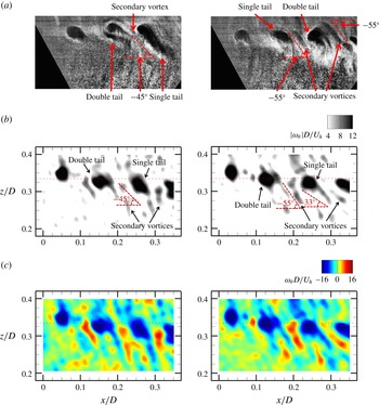
In figure 2 we compare SLPIV images (figure 2 a) with the contours of the simulated absolute value of the instantaneous azimuthal vorticity (figure 2 b) and signed instantaneous azimuthal vorticity (figure 2 c) near the bottom tip at two different time instants. The dominant features in the SLPIV snapshots in figure 2(a) are large circular voids with stretched both single and double tails. In this zoomed in view we can discern much more detail about the structure of the complex vortex cores with tails than could be deduced from figure 1. For instance, it is evident from figure 2(a) that there are two distinctly different patterns for the voids with two tails. The first is observed in the left image and appears to be composed by two distinct, albeit very closely spaced, elongated voids. The second pattern is observed in the image on the right and consists of two tails joined together to a large circular void. Another feature of the SLPIV images that is clearly evident in figure 2(a) is the presence of a second set of smaller and somewhat faint, albeit clearly visible, voids appearing in the space between the large voids with tails along the tip shear layer. For the sake of our discussion, we shall refer to these smaller voids as secondary vortices. It is important to note that even though we show herein just two representative images, the vortex patterns we have discussed appear aperiodically throughout the duration of the SLPIV flow visualization videos.
Comparison of (a) the snow voids from the high-resolution SLPIV image with (b) the absolute value and (c) the corresponding actual value of the computed instantaneous azimuthal vorticity
 $\unicode[STIX]{x1D714}_{\unicode[STIX]{x1D703}}$
from the Clipper turbine case under Inflow 2 on a streamwise-vertical plane the same as in SLPIV at two different time instants. Horizontal dashed line in the computed images shows the elevation of the bottom tip of the rotor.

In figure 2(b) we show that using the computed azimuthal vorticity magnitude as a surrogate for snow voids yields instantaneous images that exhibit essentially all patterns as those observed in the SLPIV images in figure 2(a). Namely, we observe the same distinct round tip vortex cores along the tip shear layer with the elongated comet-like tails and the weaker secondary vortices between successive tip vortices as in the field experiment. In addition to these apparent similarities, it is also seen in figure 2(b) that the inclination angles of the tip vortices with a single-tail range in this figure from 33° to 45°. While the inclination angle of the secondary vortices is approximately 55°. These ranges of values for the inclination angles are in good agreement with the field observations. To start unravelling the underlying coherent dynamics that gives rise to these complex features, we plot in figure 2(c) contours of instantaneous azimuthal vorticity to clarify the sign of vorticity associated with the various void patterns. It is evident from these figures, that the vorticity tails in the LES are associated with both negative and positive vorticity. Negative (clockwise) azimuthal vorticity marks the tip vortex cores, which, however, exhibit thin tails of negative vorticity stretched away from the cores toward the outer tip shear layer. In between the tails of the tip vortices, elongated structures of positive azimuthal vorticity also appear, giving rise to a distinct pattern of counter-rotating vortical structures aligned along the outer edge of the turbine tip shear layer. These positive vorticity structures correspond to the secondary vortices observed in figure 2(a). Figure 2(c) also clarifies the origin of the two patterns of the double-tail tip vortex cores we discussed above. It is evident that the pattern with two separate albeit closely spaced tails is associated with counter-rotating vortices. On the other hand the pattern of two tails attached to the tip vortex core is associated with vorticity of the same sign (negative vorticity in figure 2 c).
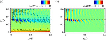
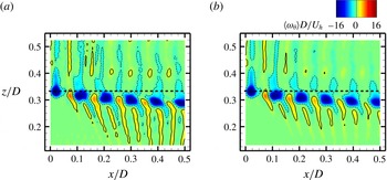
Contours of (a) phase-averaged azimuthal vorticity, and (b) the coherent part of the azimuthal vorticity on a streamwise-vertical plane passing through the rotor centre for the Clipper turbine case under Inflow 2. Horizontal black dashed line shows the elevation of rotor bottom tip. The line contours show the magnitude of the phase-averaged azimuthal vorticity
 $|\unicode[STIX]{x1D714}_{\unicode[STIX]{x1D703}}|D/U_{h}=2$
.

The above comparisons demonstrate the ability of the LES to capture vortex structures in good qualitative agreement with the SLPIV voids. They further show that the complex void patterns along the turbine tip shear layer are the result of pairs of counter-rotating vortices, namely the tip vortices with tail-like structures intertwined with elongated secondary vortical structures of opposite sign. To further probe the structure of these secondary counter-rotating vortices, we plot in figure 3(a) the contours of the phase-averaged azimuthal vorticity on the streamwise-vertical plane passing through the rotor centre. As seen in figure 3(a), the blade tip vortices with the elongated tail-like structures and the counter-rotating vortices appear clearly in an alternating manner along the turbine tip shear layer up until
 $x/D<0.5$
with the strength of the blade tip vortices being significantly larger than that of the counter-rotating vortices. Another important observation is that the phase-averaged tip vortices exhibit the distinct double-tail structure that was also observed in the instantaneous images in figure 2 and the SLPIV images (figure 1) starting at approximately
 $x=0.15D$
. Finally it is also evident from figure 3(a) that both the tip vortices and the counter-rotating vortices diminish in strength and are diffused rapidly for
 $x/D>0.5$
. To better elucidate the vortex structures near the tip, we plot in figure 3(b) the coherent part of the azimuthal vorticity (
 $\tilde{\unicode[STIX]{x1D714}}=\langle \unicode[STIX]{x1D714}\rangle -\bar{\unicode[STIX]{x1D714}}$
), which visualizes the coherent structures along the tip shear layer. Figure 3(b) clearly shows the counter-rotating vortex cores when the effect of mean shear is removed. Moreover, the tails of the positive vortex cores become more pronounced and the negative (tip vortex) cores with double tails are also observed in the contours of
 $\tilde{\unicode[STIX]{x1D714}}$
between
 $x/D=0.15$
and
 $x/D=0.25$
. We all note that figure 3 also illustrates clearly the presence of inboard vortex sheets that emanate from the trailing edge of the blade. These structures are also evident in the SLPIV images shown in figure 1.
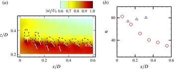
Inclination angles of phase-averaged tip vortices and secondary vortices of the Clipper turbine under Inflow 2 for (a) contours of phase-averaged streamwise velocity (flood contour) and azimuthal vorticity (black dashed lines for
 $|\unicode[STIX]{x1D714}_{\unicode[STIX]{x1D703}}|D/U_{h}=2.6$
) with inclined white lines defining the inclination of tip and secondary vortices, and (b) streamwise variation of the angles of inclination. In (a), the bottom tip of the turbine rotor is located at
 $z/D=0.33$
. The inclined direction is along the principle axis corresponding to the larger eigenvalue of the vortex shapes defined by the contour level with
 $|\unicode[STIX]{x1D714}_{\unicode[STIX]{x1D703}}|D/U_{h}=2.6$
shown in (a). The method of Peura & Iivarinen (Reference Peura, Iivarinen, Arcelli, Cordella and Di Di Baja1997) is employed to compute the principle axes of the vortex shapes in (a). In (b) the downwind coordinates of the vortices are defined as the shape centroids shown by black points in (a). In (b), red circles and blue triangles are for tip and secondary vortices, respectively.

From both LES and field measurements, we have shown that the instantaneous tip and secondary vortices are inclined forward at specific angles. In figure 4, we further examine the inclination angles of the phase-averaged vortices. As seen, the inclination angles of the tip vortices (tails for the first two tip vortices) decrease from approximately 80° to less than 30° from the first to the sixth tip vortex. This is consistent with the field observation shown in figure 1, where a high inclination angle is observed at locations near the turbine while a low inclination angle is observed further downwind. The inclination angles of the secondary vortices of approximately 80°, on the other hand, remain essentially constant in the streamwise direction. The different scaling of the inclination angles of tip and secondary vortices is related to their positions relative to the tip shear layer. The tip vortices are within the tip shear layer, while the position of the secondary vortices deviates from the tip shear layer as they are convected downstream. For the tip vortices in figure 4, the upper part of the tip vortex within the wake is convected at a low speed; the lower part outside of the wake, on the other hand, is convected at a high speed. The different convection speeds of the upper and lower parts cause the rotation of the tip vortex cores in the counter-clockwise direction and decrease the inclination angles. The convection speeds of the secondary vortices, on the other hand, are nearly the same for different parts of the vortex. This makes the inclination angle of the secondary vortices to remain nearly the same at different downstream locations.
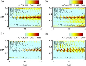
Flood contours of (a) turbulence kinetic energy, (b) streamwise turbulence intensity, (c) spanwise (azimuthal) turbulence intensity and (d) vertical turbulence intensity on a streamwise-vertical plane passing through the rotor centre for the Clipper turbine case under Inflow 2. The line contours show the magnitude of the phase-averaged azimuthal vorticity
 $|\unicode[STIX]{x1D714}_{\unicode[STIX]{x1D703}}|D/U_{h}=2$
. Horizontal black dashed line shows the location of the rotor bottom tip.

To investigate the impact of the rich dynamics we uncovered along the turbine tip shear layer on the turbulence statistics (the incoherent fluctuations in the triple decomposition), we plot in figure 5 contours of the turbulence kinetic energy (TKE), and the streamwise, spanwise (azimuthal) and vertical turbulence intensities (
 $\unicode[STIX]{x1D70E}_{u}$
,
 $\unicode[STIX]{x1D70E}_{v}$
and
 $\unicode[STIX]{x1D70E}_{w}$
). To facilitate the analysis of figure 5, we also superimpose the line contours of phase-averaged azimuthal vorticity. As seen in figure 5(a), significant increase in TKE is observed from the third blade tip vortex located between
 $x/D=0.2$
and
 $x/D=0.3$
. The regions with high TKE are mainly located within the blade tip vortices (line contours near the bottom tip). Similar trends are also observed for the streamwise (figure 5
b) and spanwise (azimuthal) (figure 5
c) components of the turbulence intensities. It is worth noting however that the spanwise (azimuthal) intensity
 $\unicode[STIX]{x1D70E}_{v}$
has lower magnitude and it starts growing rapidly further downstream than
 $\unicode[STIX]{x1D70E}_{u}$
. The vertical turbulence intensity contours, which characterize the outward stretching and transport of vortical structures along the tip shear layer, are seen in figure 5(d) to exhibit distinctly different trends than the horizontal and spanwise (azimuthal) counterparts. For instance, unlike
 $\unicode[STIX]{x1D70E}_{u}$
and
 $\unicode[STIX]{x1D70E}_{v}$
, which show a monotonic increase starting at
 $x/D\sim 0.25$
and
 $x/D\sim 0.35$
, respectively,
 $\unicode[STIX]{x1D70E}_{w}$
starts growing abruptly at
 $x/D\sim 0.15$
, continuous to increase up until
 $x/D=0.45$
, but then starts declining gradually at further downwind locations. By examining the phase-averaged vorticity distributions in figures 3(a) and 3(b), we can see that the region of drastic change in the vertical turbulence intensity corresponds to the region where the tip and the counter-rotating spiral vortices co-exist and intertwine with each other. It is also observed in figure 5(d) that the pockets of high
 $\unicode[STIX]{x1D70E}_{w}$
intensity actually connect the cores of the blade tip vortices and the counter-rotating vortices. Overall the simulated patterns of vertical turbulence intensity presented herein reveal a sudden increase in incoherent motions at approximately the location of the second tip vortex core (
 $x/D\sim 0.15$
), which is then followed with continuous increase of the TKE, especially in the area where the tip vortices lose coherence and dissipate (
 $x/D>0.5$
). This downwind increase in TKE, however, is driven by horizontal and spanwise (azimuthal) fluctuations. Vertical fluctuations are maximized in the region where the tip vortices engage in the complex interaction with the counter-rotating vortices (
 $0.15<x/D<0.5$
), which results in ejections of vorticity toward the outer part of the shear layer in the form of tail-like, elongated structures.
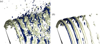
Isosurfaces of (a) instantaneous and (b) phase-averaged azimuthal vorticity
 $\unicode[STIX]{x1D714}_{\unicode[STIX]{x1D703}}$
for the Clipper turbine case under Inflow 2. The light isosurfaces show the tip vortices from the blades, while the dark isosurfaces show the counter-rotating spiral vortices. In (a), light and dark show the isosurfaces
 $\unicode[STIX]{x1D714}_{\unicode[STIX]{x1D703}}D/U_{h}=-7.8$
and 7.8, respectively. In (b), light and dark show the isosurfaces
 $\unicode[STIX]{x1D714}_{\unicode[STIX]{x1D703}}D/U_{h}=-7.8$
and 3.9, respectively. The inboard part and some azimuthal parts of the vortex system are blanked out for clarity.

The results we have presented thus far show that the vortex cores with tails observed in the SLPIV images along the turbine tip shear layer are the result of rich and highly energetic coherent dynamics characterized by pairs of counter-rotating vortices. To elucidate the three-dimensional structure of these vortices we plot in figure 6 instantaneous and phase-averaged isosurfaces of azimuthal vorticity. The negative isosurface of vorticity in figure 6 visualizes the tip vortices emanating from the blade tips. The secondary counter-rotating (positive) spiral vortices are also evident intertwined with the tip vortices in figure 6. It is also evident from figure 6(a) that the outer tip shear layer is characterized by intermittent ejections of positive and negative vorticity due to the interactions of the two sets of spiral vortices within the energetic tip shear layer. The effect of such ejection events on turbulent mixing in the tip shear layer was investigated by Lignarolo et al. (Reference Lignarolo, Ragni, Scarano, Ferreira and van Bussel2015) using quadrant analysis.
4.2 Effect of incoming turbulence
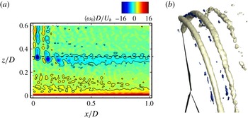
In this section, we examine the vortex structure in the near wake of the Clipper turbine under different inflow conditions. In figure 7, we visualize the vortex structures in the near wake of the Clipper turbine under Inflow 3. As seen in figure 7(a), which depicts phase-averaged azimuthal vorticity contours on a vertical plane, the secondary counter-rotating spiral vortices are still evident between the first and the second tip vortices but are hardly noticeable at further downwind locations. For the corresponding three-dimensional vortex structure shown in figure 7(b), only some fragments of the counter-rotating spiral vortices are observed suggesting that sufficiently high turbulence intensity in the incoming flow tends to rapidly diminish the coherence of the secondary spirals.
To further examine the effect of incoming turbulence, we show in figure 8 the azimuthal vorticity contours for the Clipper turbine under Inflow 4 and Inflow 5. As seen, the counter-rotating vortices computed under these two inflow conditions are significantly more elongated than those under inflows with higher turbulence intensity shown in figures 3 and 7. In comparison with the inflow without incoming synthetic turbulence (Inflow 5), the inflow with low turbulence intensity (Inflow 4) attenuates the elongation of the second set counter-rotating vortices without breaking up the overall coherence of the spiral vortices.
Vortex structure in the near wake of the Clipper turbine under Inflow 3 with
 $\unicode[STIX]{x1D70E}_{u}=\unicode[STIX]{x1D70E}_{v}=\unicode[STIX]{x1D70E}_{w}=0.094U_{h}$
for (a) contours of phase-averaged azimuthal vorticity on a streamwise-vertical plane passing through the rotor centre and (b) isosurfaces of the phase-averaged azimuthal vorticity
 $\unicode[STIX]{x1D714}_{\unicode[STIX]{x1D703}}$
. In (a),
 $|\unicode[STIX]{x1D714}_{\unicode[STIX]{x1D703}}|D/U_{h}=2$
for the contour lines. In (a), the horizontal black dashed line shows the location of the rotor bottom tip. In (b), the light isosurfaces show the tip vortices from the blades, while the dark isosurfaces show the counter-rotating spiral vortices. Light and dark show the isosurfaces
 $\unicode[STIX]{x1D714}_{\unicode[STIX]{x1D703}}D/U_{h}=-7.8$
and 3.9, respectively. The inboard part and some azimuthal parts of the vortex system in (b) are blanked out for clarity.

From the results presented in this section, we have shown that varying the turbulence intensity in the approach flow has a profound effect on the coherence and persistence of the counter-rotating spiral vortices. We found that increasing the turbulence intensity from zero to the maximum level we considered herein (Inflow 3) progressively degrades the coherence of both the tip and the secondary counter-rotating spiral vortices. The latter, however, are affected in a more profound manner since they are weaker than the blade tip vortices. That increased turbulence in the approach flow tends to diminish the strength and coherence of the primary blade-induced tip vortices has been documented in a number of previous experimental studies (Chamorro et al. Reference Chamorro, Hill, Morton, Ellis, Arndt and Sotiropoulos2013a ,Reference Chamorro, Troolin, Lee, Arndt and Sotiropoulos b , Reference Chamorro, Hill, Neary, Gunawan, Arndt and Sotiropoulos2015a ). This trend is also consistent with the analytical relationship proposed by Sarmast et al. (Reference Sarmast, Dadfar, Mikkelsen, Schlatter, Ivanell, Sørensen and Henningson2014), which shows that the downwind distance at which the tip vortices break up into small-scale turbulence depends on the ambient turbulence. We note, however, that Sarmast et al. investigated the effect of ambient turbulence on the pairing instability of the tip vortices while in our work we focus on the near-wake tip and counter-rotating vortices we have uncovered herein.
Contours of phase-averaged azimuthal vorticity of Clipper turbine on a streamwise-vertical plane passing through the rotor centre for (a) under Inflow 5 with mean streamwise velocity given by a logarithmic law without synthetic turbulence and (b) under Inflow 4 with
 $\unicode[STIX]{x1D70E}_{u}=\unicode[STIX]{x1D70E}_{v}=\unicode[STIX]{x1D70E}_{w}=0.017U_{h}$
. Solid and dashed contour lines show
 $\unicode[STIX]{x1D714}_{\unicode[STIX]{x1D703}}D/U_{h}=2.6$
and
 $-2.6$
, respectively. The horizontal black dashed line shows the location of the rotor bottom tip.

4.3 Effect of turbine design
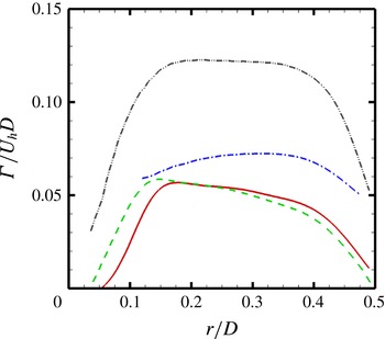
In this section, we examine the vortex structure in the near wake of four different turbines, i.e. Clipper turbine, SWiFT turbine, MEXICO turbine and the model turbine in Lignarolo et al. (Reference Lignarolo, Ragni, Scarano, Ferreira and van Bussel2015), under uniform inflow (Inflow 1). Before presenting the near-wake vortex structures, we show the non-dimensional bound circulations for the employed four turbines in figure 9. The bound circulation at
 $r$
is computed by
 $\unicode[STIX]{x1D6E4}(r)=L(r)/U_{rel}(r)$
, where
 $L(r)$
and
 $U_{rel}(r)$
are the lift force and relative incoming velocity computed from the actuator surface model. As seen, the bound circulations are very similar between the Clipper turbine and the SWiFT turbine. The bound circulation from the MEXICO turbine is larger than that from the Clipper turbine and SWiFT turbine especially in the outer part of the blade. The bound circulation from the model wind turbine, on the other hand, is significantly larger than the other three turbines (approximately two times larger for the middle part of the blade).
Bound circulations for Clipper turbine, SWiFT turbine, MEXICO turbine and the model wind turbine of Lignarolo et al. (Reference Lignarolo, Ragni, Scarano, Ferreira and van Bussel2015) under uniform inflow. Red solid line: Clipper turbine; green dashed line: SWiFT turbine; blue dash-dot line: MEXICO turbine; grey dash-dot-dot line: model wind turbine.

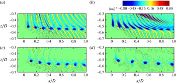
Contours of phase-averaged azimuthal vorticity on a streamwise-vertical plane passing through the rotor centre for (a) the Clipper turbine, (b) the SWiFT turbine, (c) the MEXICO turbine and (d) the model turbine of Lignarolo et al. (Reference Lignarolo, Ragni, Scarano, Ferreira and van Bussel2015) under uniform inflow. The solid and dashed contour lines show
 $\unicode[STIX]{x1D714}_{\unicode[STIX]{x1D703}}^{+}=0.05$
and
 $-0.05$
, respectively. The rotor bottom tip is located at
 $z/D=-0.5$
. In order to show the vorticity magnitude of the secondary vortices relative to the tip vortices for different turbines in the same range of contour levels, the vorticity is normalized using the maximum azimuthal vorticity magnitude of the tip vortex closest to the rotor. The values of
 $|\unicode[STIX]{x1D714}_{\unicode[STIX]{x1D703}}|D/U_{h}$
employed for normalization are 22.4, 15.7, 48.7 and 63.8 for the Clipper turbine, the SWiFT turbine, the MEXICO turbine and the model turbine, respectively.

In figure 10, we show simulated contours of the phase-averaged azimuthal vorticity for the Clipper turbine, the SWiFT turbine, the MEXICO turbine and the model wind turbine under Inflow 1. As seen in figure 10(a) for the Clipper turbine, similar vortices with a single tail or double tails as for the Inflow 2 case are observed. One major difference is that the tails together with the counter-rotating spiral vortices are now more clearly defined, persist longer in the downwind than the cases with turbulent inflow, and tend to spread radially outward starting
 $0.5D$
downstream from the turbine. This is to be anticipated, however, since increased turbulence mixing across the tip shear layer for the cases with turbulent inflow would tend to dissipate the coherent spiral vortices faster than for uniform inflow. Figure 10(a) also shows clearly the previously discussed inboard vortex sheets that originate along the span of the blade. The SWiFT turbine design exhibits overall very similar flow patterns, i.e. the single and double-tail tip vortices intertwined with the secondary counter-rotating tip vortices along the tip shear layer. One difference of the SWiFT turbine design in comparison with other turbine designs is the strong elongated vortex patterns observed within the turbine wake with
 $x/D$
from 0.4 to 0.9. Such vortex patterns originate from the blade root vortices, which is not shown in this figure. Investigation of the dependence of such vortex patterns on the blade design and the corresponding mechanism, however, is beyond the scope of this work. Secondary counter-rotating vortices are also observed for the MEXICO turbine, remain coherent for
 $x/D<0.6$
and become less organized for further downstream locations. Outward elongated counter-rotating vortices are also observed for the model wind turbine. However, the secondary counter-rotating vortices from the model turbine are not well organized at for almost all the downstream locations shown in figure 10, with their intensities being significantly smaller than the tip vortices. We do note that the experiment of Lignarolo et al. (Reference Lignarolo, Ragni, Scarano, Ferreira and van Bussel2015) did not show the emergence of the secondary counter-rotating vortices. PIV is generally limited in capturing fine velocity gradient due to the inherent smoothing associated with interrogation window and the common practice of overlapping of interrogation windows, as shown in the simulation results of the model turbine, the ratio of strength of primary and secondary vortices is close to an order of magnitude. It is possible that the PIV experiment of Lignarolo et al. (Reference Lignarolo, Ragni, Scarano, Ferreira and van Bussel2015) may not yield sufficient resolution and dynamic range to simultaneously resolve both types of vortices, as mentioned in Lignarolo et al. (Reference Lignarolo, Ragni, Scarano, Ferreira and van Bussel2015) that the PIV resolution is not high enough ‘to capture the smallest scale at the tip location’. The details of these flow patterns clearly depend on the specifics of the blade design and blade loading along the span but nevertheless the underlying basic flow features are similar across all four turbines. We observe, for instance, differences in the structure of the inboard vortex sheets, which strongly depend on the bound circulation shown in figure 9. The bound circulations from the Clipper and SWiFT turbine designs gradually decrease from
 $r/D=0.2$
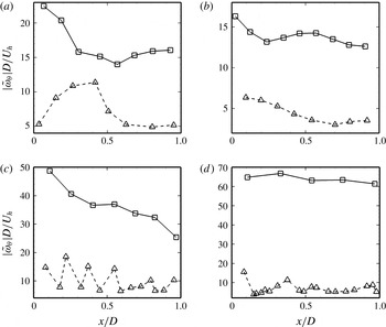
to 0.4, while the bound circulations from the MEXICO and model turbine designs remain nearly constant within the same region. Since the strength of the shed vortex sheet depends on the derivative of the bound circulation, this is consistent with the observation that the vortex sheets from the Clipper and SWiFT turbines are stronger than the other two turbines. Figure 10 shows the intensity of the secondary counter-rotating vortices relative to that of the tip vortices. To quantitatively compare the strength of the tip and secondary vortices for different turbines, we show in figure 11 the downwind variation of the maximum magnitude of phase-averaged azimuthal vorticity within the tip and secondary vortex cores normalized by
 $U_{h}/D$
. The mean values of
 $|\unicode[STIX]{x1D714}_{\unicode[STIX]{x1D703}}|D/U_{h}$
(averaged over the values shown in figure 11 for the corresponding tip and secondary vortices, respectively) of the secondary vortices for different turbines are of the same order of magnitude, which are 7.4, 4.5, 10.0 and 7.0 for the Clipper, SWiFT, MEXICO and model turbines, respectively. While the vorticity magnitude of the tip vortices of the model wind turbine is significantly larger than the Clipper turbine and the SWiFT turbine. This makes the tip vortices more dominant in the tip shear layer in comparison with the secondary counter-rotating vortices for the model wind turbine. We also note that the ratio of the maximum vorticity magnitude for the tip vortex near
 $x/D=1$
to that of the tip vortex next to the rotor is 0.95 for the model turbine. For the Clipper, SWiFT and MEXICO turbines the value of this ratio is 0.71, 0.77 and 0.52, respectively. While our results make a strong case that the specific vortex patterns depend on the blade design, such as distributions of bound circulation, blade chord and twist angle and operational conditions, the systematic investigation of these effects is beyond the scope of this work.
Downwind variation of the maximum magnitude of phase-averaged azimuthal vorticity in the tip and secondary vortex cores for (a) the Clipper turbine, (b) the SWiFT turbine, (c) the MEXICO turbine and (d) the model turbine of Lignarolo et al. (Reference Lignarolo, Ragni, Scarano, Ferreira and van Bussel2015) under uniform inflow. Solid line with squares: tip vortices; dashed line with triangles: secondary vortices. For the Clipper and SWiFT turbines, the maximum vorticity magnitude of the dominant secondary vortex corresponding to each tip vortex is extracted. No dominant secondary vortices exist in the far wake of the MEXICO turbine and in the wake of the model turbine. The maximum vorticity magnitudes of a group of secondary vortex cores corresponding to each tip vortex are extracted for these two turbines.

The results we have presented in this section clearly show that the complex large-scale dynamics along the tip shear layer of the Clipper turbine uncovered by the SLPIV field experiments and captured by LES is observed for different turbine designs. It is worth noting, for instance, that in spite of the fact that the sizes of the three field-scale turbines we have considered herein span across one order of magnitude (from the Clipper turbine to the MEXICO turbine) the overall patterns across the turbine tip shear layer are very similar.
4.4 Physical mechanisms
To our knowledge, this is the first time that such rich coherent dynamics is uncovered in the near wake of wind turbines – we note several previous studies (Okulov & Sørensen Reference Okulov and Sørensen2007; Ivanell et al. Reference Ivanell, Mikkelsen, Sørensen and Henningson2010; Iungo et al. Reference Iungo, Viola, Camarri, Porté-Agel and Gallaire2013; Sarmast et al. Reference Sarmast, Dadfar, Mikkelsen, Schlatter, Ivanell, Sørensen and Henningson2014) that have focused exclusively on the far-wake instability of the tip vortices. To identify a possible mechanism that leads to such complex coherent dynamics, we note that the flow in the wake of a wind turbine presents the potential for both shear and swirl-induced instabilities. The former could arise as a result of both axial and azimuthal shear due to the axial velocity deficit and rotor-induced azimuthal velocity in the turbine wake, respectively. The rotor-induced swirl in the turbine wake, on the other hand, also raises the possibility of centrifugal instabilities. In fact examining the simulated radial profile of the mean circulation in the turbine near wake we find that it decreases with radius in the outer part of the rotor tip shear layer. Thus, the potential for centrifugal instability of the swirling turbine wake is certainly present at least in accordance to the classical theory by Rayleigh (Reference Rayleigh1917) for purely swirling flows. A number of previous studies of related canonical flows have in fact demonstrated the potential for both shear (Kelvin–Helmholtz) and centrifugal instabilities to occur and compete with each other in swirling jets and wakes (Martin & Meiburg Reference Martin and Meiburg1996; Loiseleux, Chomaz & Huerre Reference Loiseleux, Chomaz and Huerre1998; Loiseleux, Delbende & Huerre Reference Loiseleux, Delbende and Huerre2000; Gallaire & Chomaz Reference Gallaire and Chomaz2003). We note, however, that a major difference between the present flow and previously studied canonical swirling flows is that in the wind turbine wake case a specified number of vortices of a given sign are already imposed by the rotor in the form of the spiral tip vortices. As a result, it is possible that the instability manifests itself in the form of a secondary set of weaker counter-rotating spiral vortices, which interact with the tip vortices and are stretched in the outer part of the tip shear layer giving rise to the distinct tail-like features observed in the snow visualization.
To probe deeper into the nature of the instability we have uncovered herein, we examine the stability of the computed mean flow in the turbine wake using the criterion proposed by Leibovich & Stewartson (Reference Leibovich and Stewartson1983) for studying the stability of axisymmetric vortices with axial flow. This criterion assumes inviscid flow and ignores the streamwise variation of the mean velocity field. According to Leibovich & Stewartson (Reference Leibovich and Stewartson1983), an axisymmetric vortex with axial flow is centrifugally unstable if
 $$\begin{eqnarray}C_{LS}=V_{\unicode[STIX]{x1D703}}\frac{\text{d}\unicode[STIX]{x1D6FA}}{\text{d}r}\left[\frac{\text{d}\unicode[STIX]{x1D6FA}}{\text{d}r}\frac{\text{d}\unicode[STIX]{x1D6E4}}{\text{d}r}+\left(\frac{\text{d}U}{\text{d}r}\right)^{2}\right]<0,\end{eqnarray}$$
where
 $V_{\unicode[STIX]{x1D703}}(r,~x)$
is the time- and azimuthal-averaged azimuthal velocity,
 $U(r,~x)$
is the time- and azimuthal-averaged axial velocity,
 $\unicode[STIX]{x1D6FA}(r,~x)$
is the time- and azimuthal-averaged angular velocity and
 $\unicode[STIX]{x1D6E4}(r,~x)$
is the circulation
 $\int _{0}^{2\unicode[STIX]{x03C0}}rV_{\unicode[STIX]{x1D703}}\,\text{d}\unicode[STIX]{x1D703}$
(
 $\unicode[STIX]{x1D703}$
is the azimuthal angle).
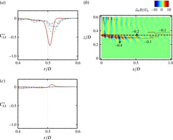
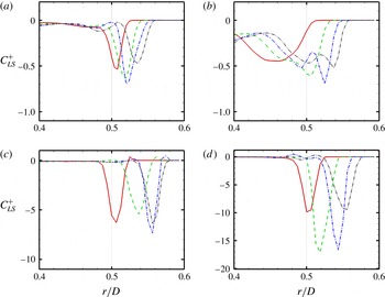
In figure 12(a), we plot the mean radial profiles of
 $C_{LS}$
at
 $0.1D$
,
 $0.3D$
,
 $0.5D$
and
 $0.7D$
turbine downwind for the Clipper turbine under Inflow 2. As seen, the
 $C_{LS}$
becomes negative within the tip shear layer with the location of its minimum moving radially outward and its magnitude diminishing with distance from the turbine tip. In figure 12(b), we plot the flood contours of the coherent part of the azimuthal vorticity superimposed with line contours of
 $C_{LS}$
of the Clipper turbine case under Inflow 2. It is evident from this figure that the region within which
 $C_{LS}$
becomes negative and the instability criterion is satisfied coincides with the edge of the turbine tip shear layer and the location of the counter-rotating spiral vortices. For the Clipper turbine case under high turbulence intensity inflow (Inflow 3) shown in figure 12(c), on the other hand, the magnitude of
 $C_{LS}$
is very small and no peak with minimum
 $C_{LS}$
exists near the blade tip, although the
 $C_{LS}$
is also negative there. This is consistent with the very weak counter-rotating vortex structure observed for the Clipper turbine case under Inflow 3 shown in figure 7.
(a), (c) Mean radial profiles of
 $C_{LS}$
at different downwind locations:
 $0.1D$
(solid line);
 $0.3D$
(dashed line);
 $0.5D$
(dash-dot line);
 $0.7D$
(dash-dot-dot line) for the Clipper turbine cases under Inflow 2 and Inflow 3, respectively. (b) Flood contours of the coherent part of the azimuthal vorticity and line contours of the
 $C_{LS}$
for the Clipper turbine case under Inflow 2 (only the
 $C_{LS}$
contours near the bottom tip are plotted for clarity) on a streamwise-vertical plane passing through the rotor centre. The
 $C_{LS}$
is normalized using
 $D$
and
 $U_{h}$
as the characteristic length and velocity scales, respectively.

To further demonstrate that the theory of Leibovich & Stewartson (Reference Leibovich and Stewartson1983) can be used to qualitatively predict the appearance of the counter-rotating vortices in the turbine tip shear layer, we show in figure 13 the variation of
 $C_{LS}$
for the four turbine designs under uniform inflow (Inflow 1). It is evident from figure 13(a) that for the Clipper turbine the
 $C_{LS}$
profiles vary in a similar manner as for Inflow 2. Namely, we observe: (i) minimum negative peaks within the tip shear layer; (ii) nearly zero
 $C_{LS}$
values outside of the tip shear layer; and (iii) radially outward movement of the location of the minimum peaks. The main difference observed between the Inflow 1 and Inflow 2 cases is that for the former (figure 13
a) the
 $C_{LS}$
magnitude increases slightly from
 $x/D=0.1$
to
 $x/D=0.5$
whereas it decreases for the latter case (figure 12
a). Figures 13(b) and 13(d) reveal overall similar variations of
 $C_{LS}$
for the SWiFT turbine, MEXICO turbine and model wind turbine. Namely, that for all the three turbine designs the region within which
 $C_{LS}$
becomes negative follows well the tip shear layer. This figure also reveals some design-specific differences. For the SWiFT turbine case: (i) the minimum peak at
 $0.1D$
turbine downwind appears at a radial location less than
 $0.5D$
; and (ii) the width of the region with negative
 $C_{LS}$
is larger than that of the Clipper turbine and the MEXICO turbine. For the MEXICO turbine case: (i) the radial displacement of the minimum peak from
 $0.1D$
to
 $0.7D$
turbine downwind is larger than that of the Clipper turbine and the SWiFT turbine because of the larger wake expansion; and (ii) a very narrow region with positive
 $C_{LS}$
exists just after the minimum peak of
 $C_{LS}$
in radial direction. For the model turbine case: (i) the magnitude of
 $C_{LS}$
is significantly larger than that of the Clipper turbine and the SWiFT turbine; and (ii) a very narrow region with positive
 $C_{LS}$
exists just before the
 $C_{LS}$
becomes negative in radial direction. These differences notwithstanding, it is evident from figure 13 that the theory of Leibovich & Stewartson (Reference Leibovich and Stewartson1983) can qualitatively predict with consistency the onset of counter-rotating spirals in the tip shear layer for all four designs. We notice that the magnitude of
 $C_{LS}$
is not directly correlated with the strength of the secondary vortices. The magnitude of
 $C_{LS}$
of the model turbine is an order of magnitude larger than those of the Clipper and SWiFT turbines. While the intensities of the secondary vortices of these turbines are of the same order of magnitude as shown in figure 11.
Radial profiles of
 $C_{LS}$
at different downwind locations:
 $0.1D$
(solid line);
 $0.3D$
(dashed line);
 $0.5D$
(dash-dot line);
 $0.7D$
(dash-dot-dot line) for (a) the Clipper turbine, (b) the SWiFT turbine, (c) the MEXICO turbine and (d) the model turbine of Lignarolo et al. (Reference Lignarolo, Ragni, Scarano, Ferreira and van Bussel2015) under uniform inflow (Inflow 1). The
 $C_{LS}$
is normalized using
 $D$
and
 $U_{h}$
as the characteristic length and velocity scales, respectively.

The apparent success of the theory of Leibovich & Stewartson (Reference Leibovich and Stewartson1983) to qualitatively predict the onset of rich coherent dynamics along the turbine tip shear layer makes a strong case that the emergence of counter-rotating spiral vortices is the manifestation of swirl-induced centrifugal instability. Our findings further point to the conclusion that the circular voids with comet-like tails identified by the SLPIV experiments arise by the interaction of the tip vortices with the counter-rotating spiral vortices in the centrifugally unstable turbine tip shear layer, which are sheared and inclined forward by the outer flow. We emphasize that the analysis using the theory of Leibovich & Stewartson (Reference Leibovich and Stewartson1983) is inherently qualitative in nature and it is intended to provide evidence in support of our assertion that centrifugal instability is the main driver of the complex coherent dynamics we uncover in the rotor tip shear layer. More specifically, we note that the theory of Leibovich & Stewartson (Reference Leibovich and Stewartson1983) has been developed for generic swirling flows, it is performed on the time-averaged flow and as such it cannot take into account the effect of the tip vortices in the wake.
5 Concluding remarks
Field observations using snow visualization and SLPIV in the wake of a 2.5 MW Clipper turbine revealed the presence of spiral tip vortices with elongated single or double tails along with secondary vortical structures within the tip shear layer. To elucidate these complex vortex patterns and elucidate their underlying physical mechanism, we carry out LES using an actuator surface model for the blades. The computed vortex structures show qualitatively good agreement with the field visualizations. From the LES results, we have found that the complex vortex structures observed in the field are a result of the occurrence of counter-rotating spiral vortices and their interactions with the tip vortices. To further investigate the occurrence and origin of the observed complex vortex structures for different inflow conditions and different turbine designs, we carried out simulations for various inflow conditions and additional two field-scale turbine designs and one model turbine design. We observed the onset of counter-rotating spirals for all the cases. However, the strength of the counter-rotating vortices is much weaker for the model wind turbine or when the incoming turbulence intensity is high.
We showed that the theory of Leibovich & Stewartson (Reference Leibovich and Stewartson1983) can qualitatively predict the emergence of counter-rotating spirals. This finding led us to postulate that centrifugal instability of the rotating rotor tip shear layer is the primary mechanism for explaining the emergence of counter-rotating spiral vortices, although we cannot entirely exclude potential shear effects in both the axial and azimuthal directions.
The simulations with uniform flow, and for four different turbine designs, clearly show that both tip vortices and counter-rotating vortices persist in the downwind direction with no evidence of near-wake break up of tip vortices due to the presence of the counter-rotating vortices. On the other hand, the simulations with increasing inflow turbulence levels clearly show that ambient turbulence appears to play a dominant role in breaking up the tip vortices and attenuate the counter-rotating vortices–the latter are more profoundly impacted by ambient turbulence because they are weaker than the tip vortices. This finding is consistent with previous experimental and computational studies, which have shown that ambient turbulence can have a major impact on the coherent dynamics of wind turbine wakes (Chamorro et al. Reference Chamorro, Hill, Morton, Ellis, Arndt and Sotiropoulos2013a ,Reference Chamorro, Troolin, Lee, Arndt and Sotiropoulos b ; Sarmast et al. Reference Sarmast, Dadfar, Mikkelsen, Schlatter, Ivanell, Sørensen and Henningson2014; Chamorro et al. Reference Chamorro, Hill, Neary, Gunawan, Arndt and Sotiropoulos2015a ).
Our findings point to the conclusion that the tip vortices with elongated tails and the counter-rotating spiral vortices may be ubiquitous for wind turbines at all scales at least for a certain range of ambient atmospheric conditions characterized by moderate turbulence intensities. We note, however, that with only exception the work of Hong et al. (Reference Hong, Toloui, Chamorro, Guala, Howard, Riley, Tucker and Sotiropoulos2014) such phenomena have not observed in previous wind-tunnel-scale experiment (Hu et al. Reference Hu, Yang and Sarkar2012; Sherry et al. Reference Sherry, Nemes, Jacono, Blackburn and Sheridan2013; Zhang et al. Reference Zhang, Markfort and Porté-Agel2013; Howard et al. Reference Howard, Hu, Chamorro and Guala2015; Wang et al. Reference Wang, Ozbay, Tian, Sharma and Hu2015; Lignarolo et al. Reference Lignarolo, Ragni, Scarano, Ferreira and van Bussel2015). This is attributed to the lack of field-scale visualizations (Hong et al. Reference Hong, Toloui, Chamorro, Guala, Howard, Riley, Tucker and Sotiropoulos2014) and the fact that at model scale, the secondary vortices may be too weak to resolve with PIV experiments. Our findings point to the need for more focused wind tunnel experiments seeking to carefully elucidate the dynamics of turbine tip shear layer in wind tunnel studies.
Acknowledgements
This work was supported by Department of Energy DOE (DE-EE0002980, DE-EE0005482 and DE-AC04-94AL85000), Sandia National Laboratories (Sandia National Laboratories is a multi-program laboratory managed and operated by Sandia Corporation, a wholly owned subsidiary of Lockheed Martin Corporation, for the U.S. Department of Energy’s National Nuclear Security Administration under contract DE-AC04-94AL85000.), Xcel Energy through the Renewable Development Fund (grant RD4-13) and NSF Career Award (NSF-CBET-1454259) for J.H. Computational resources were provided by Sandia National Laboratories, National Renewable Energy Laboratory, and the University of Minnesota Supercomputing Institute.
Appendix A. Computation of turbulence intensity from the field measurement data
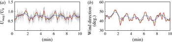
In order to justify the turbulence intensity employed in the Inflow 2 state for the LES of the Clipper turbine, the turbulence intensities of the approach atmospheric flow during the SLPIV field experiments are analysed in this appendix. As shown in figure 14, both wind speed and wind direction change significantly during the considered time period. Directly computing the turbulence intensity from these time series will incorrectly regard these large-scale wind speed and wind direction variations as turbulent fluctuations. In order to at least partly remove the effects of such large-scale variations, a moving-average approach is employed to compute the turbulence intensity for different time intervals centred at each time instants. The purpose of this approach, however, is not to compute the turbulence intensity accurately for each time intervals, but to get a rough estimation on the range of the turbulence intensity during SLPIV experiment.
Variations of (a) the magnitude of the measured wind velocity and (b) the measured wind direction at 30 m above the ground. The velocity magnitude is normalized using the corresponding moving-average velocity magnitude at 80 m above the ground. The wind direction is calculated using the moving-average wind velocity as 30 m above the ground. The grey dotted lines in (a) show the original values without moving average. Red solid line:
 $N=300$
; Green dashed line:
 $N=600$
; Blue dashed line:
 $N=1200$
. For clarity reason, only ten minutes time series are shown in this figure.

Let us define
 $M$
as the number of total samples and
 $N$
the number of the samples employed for each subset of the moving average. The moving-average value
 $\langle u_{N,E,z}\rangle _{M}$
of
 $u_{N,E,z}$
at a time instant
 $m$
is then calculated as
 $$\begin{eqnarray}\langle u_{N,E,z}\rangle _{M}(m)=\frac{1}{N}\mathop{\sum }_{n=m-N/2}^{m+N/2-1}u_{N,E,z}(n),\end{eqnarray}$$
for each velocity components, where
 $u_{N,E,z}$
denote the velocity components in the north–south, east–west and vertical directions, respectively, and
 $\langle \rangle _{M}$
denotes the moving-average operation. Using the computed
 $\langle u_{N,E,z}\rangle _{M}$
, the corresponding root-mean-square of the fluctuations at the time instant
 $m$
is then calculated as
 $$\begin{eqnarray}\unicode[STIX]{x1D70E}_{u_{N,E,z}}(m)=\left(\frac{1}{N}\mathop{\sum }_{n=m-N/2}^{m+N/2-1}(u_{N,E,z}(n)-\langle u_{N,E,z}\rangle _{M}(m))^{2}\right)^{1/2},\end{eqnarray}$$
for each velocity components.
Using the procedure described above, the wind velocity data collected at 30 m and 80 m above the ground from the sonic anemometers installed on a met tower 160 m south of the Clipper turbine are employed to calculate the turbulence intensity and wind speed during 3:00 to 3:30 am on 22 February, 2013. The number of total samples
 $M$
equals 36 000 for the 30 min data collected from the 20 Hz sonic anemometer. Three different values of
 $N$
, i.e. 300, 600 and 1200, which correspond to 15 s, 30 s and 60 s time intervals, respectively, are considered.
The variations of the corresponding magnitude of the wind velocity and the wind directions for ten minutes are plotted in figure 14. The computed minimum, maximum and mean values of the turbulence intensities are listed in table 1 for different
 $N$
values. As seen, the turbulence intensities range from
 $0.038U_{h}$
to
 $0.256U_{h}$
,
 $0.049U_{h}$
to
 $0.364U_{h}$
and
 $0.031U_{h}$
to
 $0.141U_{h}$
for the north–south, east–west and vertical velocity components, respectively. Since the pairing and merging of tip vortices, and more complex vortex patterns are also observed in the turbine’s near wake during the SLPIV experiment (shown in figure 1 and 2 in the paper of Hong et al. (Reference Hong, Toloui, Chamorro, Guala, Howard, Riley, Tucker and Sotiropoulos2014)), the lower limit of the turbulence intensity (
 $\unicode[STIX]{x1D70E}_{u}=\unicode[STIX]{x1D70E}_{v}=\unicode[STIX]{x1D70E}_{w}=0.047U_{h}$
for Inflow 2) should be more representative for the scenario interested in this paper that the tip vortices are well ordered along the tip shear layer.
Measured turbulence intensities at 30 m above the ground, where
 $\unicode[STIX]{x1D70E}_{u_{N}}$
,
 $\unicode[STIX]{x1D70E}_{u_{E}}$
and
 $\unicode[STIX]{x1D70E}_{u_{z}}$
denote the turbulence intensities for velocity components in the north–south, east–west and vertical directions, respectively. The turbulence intensity is normalized using the corresponding moving-average velocity magnitude at 80 m above the ground.

Appendix B. Validation of the actuator surface model in predicting the strength of tip vortices
In this appendix, we evaluate the capability of the actuator surface blade model we have employed herein to predict the tip vortices. We compare the computed tip vortex results with the measurements reported in the literature for the MEXICO turbine case (Snel, Schepers & Montgomerie Reference Snel, Schepers and Montgomerie2007; Shen et al.
Reference Shen, Zhu and Sørensen2012; Nilsson et al.
Reference Nilsson, Shen, Sørensen, Breton and Ivanell2015). The tip speed ratio is 6.7 as presented in the § 4. Three different computational domains are considered: (i)
 $L_{x}\times L_{y}\times L_{z}=4.2D\times 4D\times 4D$
; (ii)
 $L_{x}\times L_{y}\times L_{z}=4.2D\times 2D\times 2D$
; and (iii)
 $L_{x}\times L_{y}\times L_{z}=6.2D\times 2D\times 2D$
. The turbine is placed at
 $1.2D$
from the inlet plane. The mesh is uniform in the streamwise direction with grid spacing
 $\unicode[STIX]{x0394}x=D/160$
. The mesh in the other two directions is uniform across the rotor with grid spacing
 $D/160$
and is stretched away from the rotor. The size of time step is
 $T/750$
where
 $T=2\unicode[STIX]{x03C0}/\unicode[STIX]{x1D6FA}$
is the rotational period of the rotor and
 $\unicode[STIX]{x1D6FA}$
is the corresponding rotational speed. The inflow is uniform. The Reynolds number based on the incoming wind speed at turbine hub height and the rotor diameter is
 $6.9\times 10^{6}$
.
To examine the effect of the computational domain length in the streamwise direction, the azimuthal vorticity contours in near wake (
 $x<1D$
) for
 $L_{x}=4.2D$
and
 $L_{x}=6.2D$
, which are not shown herein, have been compared. The differences observed are found to be very minor. This indicates that the streamwise length (
 $L_{x}=4.2D$
) of the computational domain employed in this paper is large enough for the accurate simulations of the tip vortices in the near wake.
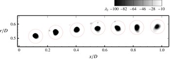
As in the paper by Nilsson et al. (Reference Nilsson, Shen, Sørensen, Breton and Ivanell2015), the tip vortex cores are identified by plotting the
 $\unicode[STIX]{x1D706}_{2}$
criterion (Jeong & Hussain Reference Jeong and Hussain1995). A visualization of the identified tip vortex cores is shown in figure 15. The sizes of the vortex cores are somewhat smaller than those predicted by Nilsson et al. (Reference Nilsson, Shen, Sørensen, Breton and Ivanell2015), but are still significantly larger than those observed in the experiment. This is inherent in the formulation of the actuator-type models, i.e. diffused distribution of the forces, and may also be partly attributed to the rather coarse mesh we employ when compared with the thickness of the blade. We note that actuator-type models are attractive exactly because of their ability to predict wind turbine wakes on grids that are too coarse to resolve the thickness of the blade. Therefore, mitigating this inherent limitation of actuator-based models is essentially impossible without using grids that are much finer than those typically employed in conjunction with such models.
Visualization of the tip vortex cores identified using the
 $\unicode[STIX]{x1D706}_{2}$
criterion, which is normalized using
 $U_{h}$
and
 $D$
. The dotted circles show the integration paths for calculating the tip vortex circulation shown in figure 16. We note that the secondary vortices uncovered in this paper can be identified using the
 $\unicode[STIX]{x1D706}_{2}$
criterion but with
 $\unicode[STIX]{x1D706}_{2}$
values of very small magnitude. For the MEXICO turbine case shown in this figure, the absolute values of
 $\unicode[STIX]{x1D706}_{2}$
for the tip vortices range from 500 to 700, while they are from 10 to 30 for the secondary vortices.

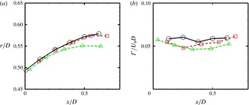
In figure 16 we compare the simulated tip vortex positions and circulation of the tip vortices with the measurements of Snel et al. (Reference Snel, Schepers and Montgomerie2007). The centre position of each tip vortex is found where
 $\unicode[STIX]{x1D706}_{2}$
is minimum within the core as in the paper by Nilsson et al. (Reference Nilsson, Shen, Sørensen, Breton and Ivanell2015). As seen in figure 16(a), the wake expansion is under predicted by the simulation with a small domain (
 $L_{y}\times L_{z}=2D\times 2D$
) in the crosswind directions. The radial positions predicted by the large domain simulation (
 $L_{y}\times L_{z}=4D\times 4D$
), on the other hand, are in good agreement with the measurements. The circulation
 $\unicode[STIX]{x1D6E4}$
, which is defined as
 $$\begin{eqnarray}\unicode[STIX]{x1D6E4}=\oint \boldsymbol{v}\boldsymbol{\cdot }\text{d}\boldsymbol{s},\end{eqnarray}$$
where
 $\boldsymbol{v}$
is the velocity vector along a closed path
 $\boldsymbol{s}$
, is compared with measurements in figure 16(b). The integration path
 $\boldsymbol{s}$
is selected as a circle centred at the centre of the tip vortex. Different radii of the integration circle have been tested by Nilsson et al. (Reference Nilsson, Shen, Sørensen, Breton and Ivanell2015). In this work, the radius of the integration circle (the red dotted circles in figure 15) is
 $0.05D$
. As seen the computed circulation of the tip vortices agree well with the measurements for both sizes of the computational domain. It is noticed that the measured radial positions and circulations of the tip vortices between
 $x=0.8D$
and
 $x=1D$
are not plotted in figure 16 for comparison due to the uncertainty of the experimental results at those locations where parts of the tip vortices were outside of the PIV photos (Nilsson et al.
Reference Nilsson, Shen, Sørensen, Breton and Ivanell2015).
Validation of the present actuator surface model in predicting the tip vortices using the experimental data of the MEXICO turbine for (a) the radial position of the tip vortices, and (b) the circulation of the tip vortices. Two different computational domain sizes are considered. The measured data were extracted from the paper by Nilsson et al. (Reference Nilsson, Shen, Sørensen, Breton and Ivanell2015). Black solid lines with circles: measurements; red dashed lines with squares: LES with
 $L_{y}\times L_{z}=4D\times 4D$
; green dash-dot lines with triangles: LES with
 $L_{y}\times L_{z}=2D\times 2D$
.