1 Introduction
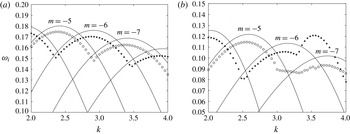
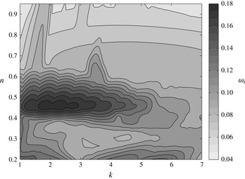
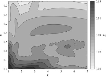
The elliptical instability of a vortex pair has received considerable attention in recent years. In particular, the short-wavelength cooperative instability exhibited by two counter-rotating vortices has been of interest. Most investigations have assumed a vortex model with no axial flow or a simple axial flow profile. We, instead, consider the elliptical instability for a family of similarity solutions found by Moore & Saffman (Reference Moore and Saffman1973). These velocity profiles are able to describe accurately both the jet-like or wake-like axial flow present in a real trailing vortex.
The short-wave cooperative instability mechanism, which can cause linear instability in a vortex subject to external strain, was first predicted by Widnall, Bliss & Tsai (Reference Widnall, Bliss and Tsai1974) for vortex rings. Shortly thereafter, Moore & Saffman (Reference Moore and Saffman1975) performed a rigorous mathematical analysis of the stability of an infinite straight vortex deformed elliptically by a weak irrotational strain field. They recognized the role of resonance in the instability process: for the case of a general axisymmetric flow, but in the absence of axial flow, they showed that two Kelvin modes can become tuned with the non-axisymmetric correction caused by the strain field. Moreover, using a multi-scale analysis in the small-strain limit, Moore and Saffman obtained estimates of the growth rate of the instability. The aforementioned authors noted that the effect of axial flow is to break the symmetry between oppositely propagating waves of the unperturbed vortex. As a consequence, the presence of an axial flow complicated the problem in such a way that their analysis could only be applied in the case of a small axial flow with a magnitude of the same order as that of the strain field. Results similar to those of Moore and Saffman were reported almost concurrently by Tsai & Widnall (Reference Tsai and Widnall1976) for the special case of a Rankine vortex.
Several years later, the short-wavelength instability was investigated again by Pierrehumbert (Reference Pierrehumbert1986), albeit in the more general framework of three-dimensional instability of two-dimensional flows. He showed that the instability occurs in a generic quadratic flow modelling the elliptically deformed rigidly rotating core of a general two-dimensional strained flow. Accordingly, the short-wave instability mechanism can be viewed more broadly to be an elliptical instability. Additionally, Pierrehumbert discovered that, in the short-axial-wavelength limit, the modal structure of the instability becomes increasingly trapped near the vortex centre while the growth rate approaches a constant value. This means that there is no short-wavelength cutoff in the absence of viscosity. In contrast, Landman & Saffman (Reference Landman and Saffman1987) determined that such a cutoff does exist in the case of a viscous flow, bounding from above the axial wavenumbers for which instability can persist. Solving a matrix Floquet problem, Bayly (Reference Bayly1986) obtained close agreement with the results of Pierrehumbert (Reference Pierrehumbert1986). Several years after the aforementioned investigations by Pierrehumbert and Bayly, Waleffe (Reference Waleffe1990) took a third approach to the same problem. He showed that the stability of the flow is governed by a second-order ordinary differential equation (ODE) known as the Ince equation, and succeeded in finding an analytical form of the modes found by Pierrehumbert and Bayly. In addition, Waleffe clarified the physical mechanism of instability as one of vortex stretching. None of the studies mentioned include axial flow, since it makes an analytical approach largely intractable. As a consequence, most analytical investigations in the last 20 years have made restrictive assumptions, such as a specific swirl flow profile
 $V(r)$
and an absence of axial flow. Several of these investigations are discussed below. A review of recent progress that has been made in elliptical instability research can be found in Kerswell (Reference Kerswell2002).
The vortical flows of interest in this paper include an axial mean flow
 $W(r)$
as well as a swirl component
 $V(r)$
. The Rankine vortex is the simplest model for the swirl component. It is given by
 $$\begin{eqnarray}V(r)=\left\{\begin{array}{@{}ll@{}}\unicode[STIX]{x1D6FA}r,\quad & \text{if}\;r\leqslant a,\\ \unicode[STIX]{x1D6FA}a^{2}/r,\quad & \text{if}\;r>a,\end{array}\right.\end{eqnarray}$$
where
 $a$
is the vortex core radius and
 $\unicode[STIX]{x1D6FA}$
is the solid body rotation rate in the core. The modal solutions corresponding to this profile are termed Kelvin waves. A detailed analysis of the elliptical instability of the Rankine vortex in a multipolar strain field is presented in Eloy & Le Dizès (Reference Eloy and Le Dizès2001). For a similar problem, the Rankine vortex in a dipolar strain field without viscosity, Fukumoto (Reference Fukumoto2003) obtained an explicit solution for the disturbance flow field using Bessel and modified Bessel functions, thus allowing for an in-depth analysis of the instability. A more realistic representation of a vortex, because its vorticity is continuous, is provided by the Lamb–Oseen vortex which has azimuthal velocity
 $V(r)=(1-\text{e}^{-r^{2}})/r$
. Le Dizès & Laporte (Reference Le Dizès and Laporte2002) considered the stability of a pair of Lamb–Oseen vortices, comparing estimates from the theory by Moore and Saffman with direct numerical results. The most unstable elliptical modes were found to be a combination of
 $m=-1$
and
 $m=1$
modes. We note that the study of the elliptical instability for the Rankine vortex and the Lamb–Oseen vortex yields very different results. For example, Sipp & Jacquin (Reference Sipp and Jacquin2003) point out that, contrary to the case of a Rankine vortex, the presence of critical layers in a Lamb–Oseen vortex prevents a large number of possible resonances. Resonant coupling between Kelvin modes with azimuthal wavenumbers
 $m=-2$
and
 $m=0$
occurs for the Rankine vortex, while the corresponding interaction is damped for the Lamb–Oseen vortex.
More recently, there has been a great deal of interest in understanding the role of elliptical instability in trailing wingtip vortices. A model more realistic than the Lamb–Oseen vortex was proposed by Fabre & Jacquin (Reference Fabre and Jacquin2004a
), who presented a two-scale model for the swirl flow
 $V(r)$
, effectively introducing an extra parameter
 $\unicode[STIX]{x1D6FC}$
to better fit trailing vortex data. It has, however, been known from flight tests for many years that aircraft trailing vortices sometimes contain strong axial flows (see, e.g., Chow, Zilliac & Bradshaw Reference Chow, Zilliac and Bradshaw1997). As shown by Lacaze, Birbaud & Le Dizès (Reference Lacaze, Birbaud and Le Dizès2005), adding a constant axial jet to the core of the Rankine vortex has a considerable influence on the combinations of Kelvin modes partaking in the resonance process. One of the few studies to consider a trailing vortex model with an axial flow is that by Lacaze, Ryan & Le Dizès (Reference Lacaze, Ryan and Le Dizès2007), which concerns the elliptical instability of the Batchelor vortex. These authors performed a systematic study of the modes of elliptical instability of a pair of counter-rotating Batchelor vortices, whose axial flow
 $W(r)=W_{0}\text{e}^{-r^{2}}$
, with
 $0<W_{0}<0.66$
. In contrast to the Lamb–Oseen vortex (
 $W_{0}=0$
), the combination of
 $m=-1$
and
 $m=1$
Kelvin modes becomes damped for a slight axial flow. Other resonant pairs become successively unstable and stable as the axial flow is increased further. The stability of a pair of co-rotating Batchelor vortices was subsequently studied by Roy et al. (Reference Roy, Schaeffer, Le Dizès and Thompson2008). Three years later, the findings for co- and counter-rotating Batchelor vortices were compared with measurements made using particle image velocimetry in a water tank (Roy et al.
Reference Roy, Leweke, Thompson and Hourigan2011). The experiment revealed a short-wave instability with a spatial structure characterized by the
 $m=0$
and
 $|m|=2$
azimuthal Fourier modes.
Despite the fact that it is now recognized that the presence of axial flow has a noticeable effect on the elliptical instability, there have been no previous investigations that account for the diversity of axial flow that can be present in trailing vortices. Even though the gathering of inflight data of trailing vortices is difficult, Brown (Reference Brown2014) has performed measurements by traversing the wake of a DC-8 airliner at high altitude. His results show axial velocities that are strong and have profiles that can be both jet-like and wake-like at different values of the radial coordinate (see his figure 6). He further reports the observation of short-wavelength instability in pairs of such vortices. Brown’s findings, together with our personal communication with him, helped to motivate us in the present study.
We now review several elements from the introduction of Feys & Maslowe (Reference Feys and Maslowe2014). The relative axial velocity in a trailing vortex can be directed towards the aeroplane (wake-like) or away from it (jet-like). Although the latter may seem unexpected, Spalart (Reference Spalart1998) offers two mathematical explanations for jet-like flow, using either the shape of the vortex lines or the Bernoulli equation and the pressure (an argument already given by Batchelor (Reference Batchelor1964)). He also points out that the axial flow can be not only wake-like or jet-like, but it can switch sign within the same flow. The far-field solution found by Batchelor does not account for this range of possibilities. In addition, the effect of vortex wandering on experimental observations must be recognized (Baker et al.
Reference Baker, Barker, Bofah and Saffman1974). Devenport et al. (Reference Devenport, Rife, Liapis and Follin1996) explain that the velocity field of any vortex will appear as a Batchelor vortex given sufficient wandering. Motivated by the ability of the family of similarity solutions found by Moore & Saffman (Reference Moore and Saffman1973) to account for both wake- and jet-like flows, our objective is to use these mean flow profiles for an analysis of the elliptical instability of a trailing vortex. It was pointed out by del Pino et al. (Reference del Pino, Parras, Felli and Fernandez-Feria2011) that the presence of an extra parameter (the wing loading parameter
 $n$
) allows for a greater variety of velocity profiles to be accurately fitted by the Moore–Saffman profiles than is the case with the Batchelor vortex. So far, only the linear inviscid stability for the Moore–Saffman profiles has been studied (Feys & Maslowe Reference Feys and Maslowe2014), yielding growth rates that are somewhat larger than those obtained for the Batchelor vortex. The instability is found to persist for larger values of the swirl. The largest amplification rates are found to occur at
 $n=0.44$
. For
 $n<0.44$
, the flow in the vortex core is jet-like and the growth rates of unstable perturbations become progressively smaller. An important question addressed in the present work is whether the same behaviour persists for the modes of elliptical instability.
The goal of this study is to investigate the elliptical instability for the base flow velocity profiles found by Moore & Saffman (Reference Moore and Saffman1973). After imposing a weak strain field on the base mean flow, the vortex streamlines relax to an elliptically deformed equilibrium state (Jiménez, Moffatt & Vasco Reference Jiménez, Moffatt and Vasco1996). For our purposes, an expression for the first-order non-axisymmetric correction to the base flow given by Moore & Saffman (Reference Moore and Saffman1975) will suffice. The resulting elliptical mean flow will then be used to perform a direct simulation in cylindrical coordinates, employing a numerical method described by Matsushima & Marcus (Reference Matsushima and Marcus1997). We will extensively compare the resulting growth rates and vorticity contours with the results for the Batchelor vortex obtained by Lacaze et al. (Reference Lacaze, Ryan and Le Dizès2007). In addition, we will relate our findings to those of Roy et al. (Reference Roy, Schaeffer, Le Dizès and Thompson2008). The effect of the wing loading parameter
 $n$
on the Moore–Saffman profiles will be thoroughly investigated. We will carry out this study in both the linearly stable and unstable regimes of the axisymmetric base flow. In the stable case, the magnitude of the axial flow will be diminished to such an extent as to prevent amplification of linear inviscid perturbations acting on the unstrained flow. Viscous modes (Khorrami Reference Khorrami1991) and centre modes (Heaton Reference Heaton2007a
) exist for lower amounts of axial flow but are not expected to have an influence on the elliptical instability mechanism and hence do not interfere with our objectives of examining the cooperative instability. The setting for a part of our investigation will be that of an unstable base flow. This results in a competition between elliptical and swirling flow instability, which we will analyse.
Our paper is organized as follows. In § 2, the Moore–Saffman profiles are introduced. We emphasize the physical effect of the wing loading parameter
 $n$
on the axial velocity component and then summarize the linear inviscid stability results for the Moore–Saffman base flow profiles in order to determine its stability characteristics for the flow parameters under consideration in the numerical simulation. In § 3, we discuss the non-axisymmetric correction caused by the strain field on the base flow and we derive the governing equation for a perturbation in the presence of viscosity. Further, the details of the numerical procedure are given in this section. We verify the numerical method by comparing its output with a multitude of published results. Section 4 contains the findings of our numerical investigation of the stability of a Moore–Saffman vortex subject to a dipolar strain field. Instability growth rates and vorticity contours are presented and compared with the results for the Batchelor vortex. The effect of a change of the wing loading parameter
 $n$
, the axial wavenumber
 $k$
and the axial flow parameter
 $W_{0}$
on the resonant pairs is of particular concern. We also consider the role played by the Reynolds number
 $Re$
and the strain rate
 $\unicode[STIX]{x1D700}$
. The parameter
 $n$
is shown to have a substantial impact on the growth rates, as discussed in the concluding remarks section (§ 5).
2 Stability characteristics of the Moore–Saffman vortex
In this section, we present the vortex profiles that will be used in our study. First, we review the family of similarity solutions of the Navier–Stokes equations found by Moore & Saffman (Reference Moore and Saffman1973). The procedure used to match these profiles, employed in the viscous core, to an inviscid outer region is detailed next. The aim, in § 4, is to study the elliptical instability of the resulting vortical flow in both the linearly stable and unstable regimes. We therefore summarize the stability characteristics of the mean velocity profiles in order to determine the flow parameters for which they are linearly stable in the absence of strain. The stability threshold is of particular interest.
2.1 Viscous inner region
Consider a columnar vortex with velocity components
 $[0,V(r),W(r)]$
in cylindrical coordinates
 $(r,\unicode[STIX]{x1D703},z)$
in an incompressible and inviscid fluid. The assumption of axisymmetry of this base flow is reasonable since it describes the mean flow in the absence of strain and, thus, without non-axisymmetric effects.
Moore & Saffman (Reference Moore and Saffman1973) began by considering the inviscid roll-up of a wingtip vortex. Because the loading of the wing is an important unknown, a wing loading parameter
 $n$
was introduced, with
 $n=1/2$
corresponding to elliptical loading,
 $0<n<1$
. In the limit where
 $n\rightarrow 1$
, Batchelor’s solution is recovered. After making the light-loading approximation, the solutions of the inviscid governing equations were shown to be singular near the vortex core. This necessitates inclusion of viscosity to describe the interior of the vortex. Using boundary layer methods, Moore and Saffman then derived parabolic governing equations and obtained a solution using a similarity variable
 $\unicode[STIX]{x1D702}=-r^{2}/(4\unicode[STIX]{x1D708}t)$
, where
 $\unicode[STIX]{x1D708}$
denotes the kinematic viscosity and
 $t$
is time. The resulting family of similarity solutions for the azimuthal and axial mean velocities is given by
 $$\begin{eqnarray}v_{\unicode[STIX]{x1D703}}(r,t)=\frac{\unicode[STIX]{x1D6FD}}{(\unicode[STIX]{x1D708}t)^{n/2}}V_{n}(\unicode[STIX]{x1D702})\quad \text{and}\quad w(r,t)=\frac{\unicode[STIX]{x1D6FD}^{2}}{W_{\infty }(\unicode[STIX]{x1D708}t)^{n}}W_{n}(\unicode[STIX]{x1D702})\end{eqnarray}$$
respectively. The constant
 $\unicode[STIX]{x1D6FD}$
is related to the wing loading, angle of attack and aspect ratio, and
 $W_{\infty }$
is the speed of the wing at infinity. It can be seen from (2.1) that the velocity components are proportional to an azimuthal function
 $V_{n}(\unicode[STIX]{x1D702})$
and an axial function
 $W_{n}(\unicode[STIX]{x1D702})$
; the exact expressions for both involve confluent hypergeometric functions. Moreover, the axial component
 $W_{n}(\unicode[STIX]{x1D702})$
is found to be the solution to a second-order ODE that must be solved numerically. Feys & Maslowe (Reference Feys and Maslowe2014) provide definitions of the functions
 $V_{n}(\unicode[STIX]{x1D702})$
and
 $W_{n}(\unicode[STIX]{x1D702})$
that were just introduced. Here, we limit ourselves to displaying the velocity components graphically.
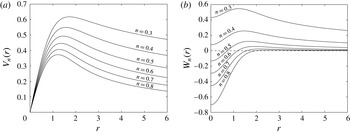
The functions
 $V_{n}(r)$
and
 $W_{n}(r)$
are shown in figure 1, where
 $r$
has been non-dimensionalized by employing a length scale
 $r_{s}=\sqrt{4\unicode[STIX]{x1D708}t}$
; the similarity variable
 $\unicode[STIX]{x1D702}$
is now related to
 $r$
by
 $\unicode[STIX]{x1D702}=-r^{2}$
. A particularly interesting aspect of the Moore–Saffman profiles is that the character of the axial component
 $W_{n}(r)$
changes near
 $n=0.44$
. For
 $n$
larger than this value, the vortex has a wake-like core with jet-like velocity only for large
 $r$
. This is consistent with Batchelor’s solution, which is recovered for
 $n\rightarrow 1$
(but corresponds to an unrealistic rectangular lift distribution) and which he described as being wake-like. As
 $n$
decreases, it can be seen that even for
 $n=0.7$
the axial velocity profile is not far from Gaussian. However, the magnitude of
 $W_{n}(0)$
decreases with
 $n$
, and for
 $n\lesssim 0.44$
, the flow relative to the wing becomes jet-like. Since experimental observations in close proximity to the wingtip have revealed both axial flow deficits and excesses, the wing loading parameter
 $n$
makes the Moore–Saffman family of profiles well suited to model the variety of axial flows present. Many factors influence the value of
 $n$
in practice because the wake- or jet-like characteristics of the vortex depend on the angle of attack and the tip configuration of the wing (see Chow et al.
Reference Chow, Zilliac and Bradshaw1997; Anderson & Lawton Reference Anderson and Lawton2003). A high angle of attack or a round wingtip generally leads to an axial velocity excess at the vortex core (jet-like flow) which corresponds to a low value of
 $n$
.
Numerical solution giving (a) the tangential velocity profile
 $V_{n}(r)$
and (b) the axial velocity profile
 $W_{n}(r)$
obtained from the similarity solution of Moore & Saffman (Reference Moore and Saffman1973).

In the numerical investigation that follows, we will non-dimensionalize the velocity profiles given by the Moore–Saffman similarity solution in a way that facilitates comparison with results for the Batchelor vortex. To that end, we begin by defining the core circulation
 $\unicode[STIX]{x1D6E4}$
to be the circulation at the radius
 $r_{m}$
(or
 $\unicode[STIX]{x1D702}_{m}$
in the similarity variable) where the azimuthal velocity reaches its peak value. (Coincidentally, Spalart (Reference Spalart1998), in discussing the decay of trailing vortices, remarks that the core circulation ‘is as legitimate as any other measure’.) It follows from (2.1) that
 $$\begin{eqnarray}\unicode[STIX]{x1D6E4}=\frac{\unicode[STIX]{x1D6FD}}{(\unicode[STIX]{x1D708}t)^{n/2}}r_{s}\unicode[STIX]{x1D6E4}_{n},\end{eqnarray}$$
where
 $\unicode[STIX]{x1D6E4}_{n}=2\unicode[STIX]{x03C0}\sqrt{-\unicode[STIX]{x1D702}_{m}}V_{n}(\unicode[STIX]{x1D702}_{m})$
is a dimensionless quantity wholly determined by the maximization of the function
 $V_{n}$
. We remark that
 $\unicode[STIX]{x1D6E4}_{n}$
depends on the value of
 $n$
, as can be inferred from figure 1(a), and must be obtained numerically since no closed-form expression is available. We will normalize all vortices by scaling them such that their core circulation is equal to the value for the Batchelor vortex, namely
 $\unicode[STIX]{x1D6E4}_{b}\simeq 4.4949$
.
We now define the length scale
 $r_{s}$
already introduced above and a characteristic velocity that will be used to scale both velocities, i.e.
 $$\begin{eqnarray}r_{s}=\sqrt{4\unicode[STIX]{x1D708}t}\quad \text{and}\quad V_{s}=\frac{\unicode[STIX]{x1D6E4}_{n}}{\unicode[STIX]{x1D6E4}_{b}}\frac{\unicode[STIX]{x1D6FD}}{(\unicode[STIX]{x1D708}t)^{n/2}}.\end{eqnarray}$$
The Reynolds number defined by these scales is
 $Re=r_{s}V_{s}/\unicode[STIX]{x1D708}$
. It depends on the wing loading parameter
 $n$
in two ways. First, the constants
 $\unicode[STIX]{x1D6FD}$
and
 $\unicode[STIX]{x1D6E4}_{n}$
in the definition of
 $V_{s}$
vary slowly with
 $n$
. Second, the disparate nature of viscous diffusion on the length and velocity scales in (2.3), to wit
 $r_{s}\sim \sqrt{\unicode[STIX]{x1D708}t}$
and
 $V_{s}\sim (\unicode[STIX]{x1D708}t)^{-n/2}$
, causes the Reynolds number to be a different function of
 $\unicode[STIX]{x1D708}t$
for every value of
 $n$
. Regarding the latter comment, we will freeze the vortex flow in time (see § 3.1), which means fixing a time
 $t$
in (2.3).
In order to ensure that Batchelor’s model is approximated in the limit
 $n\rightarrow 1$
, we will insert the quantity
 $\bar{W}$
, which is the difference between the maximum and minimum of
 $W_{n}$
, into the expression for the axial velocity component only. The corresponding quantity for the Batchelor vortex is
 $\bar{W}_{b}=1$
. Taking
 $r_{s}$
and
 $V_{s}$
as in (2.3), the non-dimensionalized profiles that result are
 $$\begin{eqnarray}V(r)=\frac{\unicode[STIX]{x1D6E4}_{b}}{\unicode[STIX]{x1D6E4}_{n}}V_{n}(\unicode[STIX]{x1D702})\quad \text{and}\quad W(r)=W_{0}\frac{\bar{W}_{b}}{\bar{W}}W_{n}(\unicode[STIX]{x1D702}),\end{eqnarray}$$
with
 $\unicode[STIX]{x1D702}=-r^{2}$
and a dimensionless axial flow parameter
 $W_{0}$
given by
 $$\begin{eqnarray}W_{0}=\frac{\unicode[STIX]{x1D6E4}_{b}}{\unicode[STIX]{x1D6E4}_{n}}\frac{\unicode[STIX]{x1D6FD}}{W_{\infty }(\unicode[STIX]{x1D708}t)^{n/2}}\frac{\bar{W}}{\bar{W}_{b}}.\end{eqnarray}$$
The introduction of an axial flow parameter
 $W_{0}$
contrasts with the more common convention in the literature on vortex stability (Lessen, Singh & Paillet Reference Lessen, Singh and Paillet1974; Mayer & Powell Reference Mayer and Powell1992), where the magnitude of the axial velocity is normalized and a swirl parameter
 $q$
is introduced. Both are related in a straightforward way by
 $W_{0}=1/q$
. There are two reasons why the use of
 $W_{0}$
is preferable if one wishes to study the elliptical instability of the strained vortex. First, since the axial component
 $W(r)$
can be viewed as having a destabilizing effect on a stable vortex
 $V(r)$
in an unbounded domain, one expects the flow to be stable for
 $W_{0}<W_{0,c}$
, where
 $W_{0,c}$
is the stability threshold of the axial flow parameter. By using an axial flow parameter, calculations can be performed for a bounded interval of values of
 $W_{0}$
to get a complete picture of the elliptical instability in a linearly stable regime. We thus avoid having to deal with the unbounded interval
 $q>q_{c}$
. It should be noted that in the case of the Batchelor vortex, it was established by Lessen et al. (Reference Lessen, Singh and Paillet1974) that
 $q_{c}\simeq 1.5$
. This relates to a value of
 $W_{0,c}\simeq 0.66$
.
A second reason for using
 $W_{0}$
will become clear in § 3.1; the non-axisymmetric correction term induced by the strain field is, at first order, invariant to a rescaling of the azimuthal velocity. A change in
 $q$
therefore does not affect the strain field, making an axial flow parameter more appropriate for studying the stability of a strained vortex.
The Moore–Saffman family of velocity profiles describes vortices that develop from laminar flow over a wing. However, in free flight, where the Reynolds number may exceed
 $10^{6}$
, the airfoil boundary layer is likely to be turbulent. This motivated Phillips (Reference Phillips1981) to consider trailing vortices undergoing roll-up behind a lightly loaded wing on which the boundary layer is turbulent. Phillips determined the form of the Reynolds-stress distribution after identifying three regions in the vortex core. He then suggested that two modes for the decay of the peak azimuthal velocity in time are possible:
 ${\sim}t^{-n/2}$
, which is the rate for the profiles defined in this section, and
 ${\sim}t^{(n-2)/2}$
, a rate to which the decay may asymptote after some time (further behind the wingtip). Here,
 $t$
denotes time and
 $n$
is the wing loading parameter.
2.2 Inviscid outer region
The large-
 $r$
asymptotic behaviour of
 $V(r)$
and
 $W(r)$
in (2.4) is
 $$\begin{eqnarray}V(r)\sim r^{-n}\quad \text{and}\quad W(r)\sim r^{-2n},\end{eqnarray}$$
so that the circulation at infinity is unbounded for
 $n<1$
. This contrasts with other vortex models, such as the Batchelor vortex, which have a finite circulation. In order to make a comparison with those models more natural, the velocity profiles in (2.4) are matched to an inviscid outer solution by writing
 $$\begin{eqnarray}\tilde{V}(r)=\frac{V(r)}{\left(1+\left({\displaystyle \frac{r}{a}}\right)^{4}\right)^{(1-n)/4}}\quad \text{and}\quad \tilde{W}(r)=\frac{W(r)}{\left(1+\left({\displaystyle \frac{r}{a}}\right)^{4}\right)^{(1-n)/2}},\end{eqnarray}$$
where
 $a$
is a non-dimensional parameter that controls the viscous core radius. The velocity profiles in (2.7) involve a smooth transition from the Moore–Saffman profiles, in the vortex core near
 $r=0$
, to
 $$\begin{eqnarray}\tilde{V}(r)\sim \frac{1}{r}\quad \text{and}\quad \tilde{W}(r)\sim \frac{1}{r^{2}},\quad \text{for}\;r\rightarrow \infty .\end{eqnarray}$$
The form of the first formula in (2.7) closely resembles that of the second vortex model considered by Fabre & Jacquin (Reference Fabre and Jacquin2004a ). In all that follows, we will omit writing the tilde in (2.7) and (2.8).
The foregoing matching procedure impacts the far field and has little bearing on the viscous solution in the vortex core. For instance, for
 $n=0.5$
, the denominator in (2.7) affects the azimuthal velocity of the Moore–Saffman solution at
 $r=a/2$
by less than 1 % and its axial velocity at the same radius by approximately 1.5 %. The difference between the Moore–Saffman profiles from § 2.1 and their matched counterparts in (2.7) vanishes for
 $a\rightarrow \infty$
. Moreover, the concentration of the velocity profiles near the vortex centre on display in figure 1, combined with the comments at the start of this paragraph, suggests that the dependence of numerical results on
 $a$
may already be weak for
 $a\lesssim 6$
. Even so, the parameter
 $a$
must be chosen sufficiently large to prevent the outer region from encroaching on the viscous core. For more details about the effect of
 $a$
on the results of our calculations, we refer the reader to § 3.3.
2.3 Linear stability of a single vortex
Varying the wing loading parameter
 $n$
in the Moore–Saffman vortex model significantly impacts the linear stability characteristics (Feys & Maslowe Reference Feys and Maslowe2014). The key stability properties are reviewed here. They differ from those in the aforementioned investigation because the present paper includes the core circulation in the velocity scale (see § 2.1). Even so, the perturbation form of the governing equations considered in this section is the same as in Feys & Maslowe (Reference Feys and Maslowe2014). The mean profiles as
 $n\rightarrow 1$
correspond to the Batchelor vortex mean flow profiles up to an accuracy of
 $10^{-3}$
. The growth rates and regions of instability for the Batchelor vortex have been documented extensively (Mayer & Powell Reference Mayer and Powell1992; Ash & Khorrami Reference Ash, Khorrami and Green1995), and our findings are in very good agreement with those results. It should be noted that we have exchanged the swirl parameter
 $q$
for the axial flow parameter
 $W_{0}=1/q$
, as was stated in § 2.1, and that this causes the growth rates to scale by a factor of
 $W_{0}$
. The effect of viscosity on the inviscid modes of instability is illustrated. Many linear modes of instability of the Moore–Saffman vortex possess a critical layer singularity. The existence and role of the critical layer are briefly discussed at the end of this section.
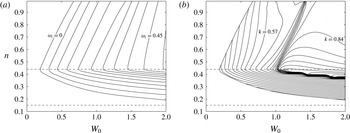
For azimuthal wavenumber
 $m=-1$
, both (a) the growth rate
 $\unicode[STIX]{x1D714}_{i}$
and (b) the corresponding axial wavenumber
 $k$
for the most unstable inviscid modes for all values in the
 $(W_{0},n)$
-plane are displayed. The contour spacing is 0.05 in (a) and 0.03 in (b), with the outermost contour representing the neutral curve. The horizontal dotted lines mark
 $n=0.44$
and
 $n=0.15$
.

With regard to the inviscid instability of the Moore–Saffman family of velocity profiles, figure 2 displays the growth rates and axial wavenumbers of the most amplified
 $m=-1$
disturbances at every point in the
 $(W_{0},n)$
-plane. First, we discuss figure 2(a). The contours on this figure are curves of constant growth rate, and the outermost contour represents the neutral curve (corresponding to
 $W_{0,c}$
). The fastest growing mode was calculated independently for every value of the axial flow parameter and the wing loading parameter; each point on the figure represents the growth rate
 $\unicode[STIX]{x1D714}_{i}$
of the most unstable perturbation for fixed values of
 $W_{0}$
and
 $n$
. For example, the most unstable disturbance for
 $W_{0}=1$
and
 $n=0.50$
has a growth rate of
 $\unicode[STIX]{x1D714}_{i}\simeq 0.2595$
. Several conclusions are true for all values of the wing loading parameter
 $n$
. The axial component
 $W(r)$
has a destabilizing effect. For
 $W_{0}=0$
, the purely swirling flow is stable for all values of
 $n$
in the sense that all disturbances decay in time. The flow destabilizes when the axial flow parameter
 $W_{0}$
is increased past a critical value
 $W_{0,c}$
. As mentioned in § 2.1,
 $W_{0,c}\simeq 0.66$
for
 $n=0.95$
, a value of the wing loading parameter for which the Moore–Saffman profiles closely correspond to those of the Batchelor vortex. For
 $n=0.50$
, the threshold has decreased to approximately
 $W_{0,c}\simeq 0.24$
. Increasing
 $W_{0}$
past the critical value results in a further destabilization of the linear inviscid modes and an increase of the growth rate of the most amplified disturbance. Two important features of the Moore–Saffman vortex model are visible. First, a decrease in
 $n$
is associated with a decrease in the critical value
 $W_{0,c}$
. This is true until
 $n=0.44$
, a constant that is indicated by the upper horizontal dotted line. The special significance of this value of the wing loading parameter can be understood from figure 1(b): the change in sign of the core axial velocity at
 $n=0.44$
corresponds to a transition from wake-like to jet-like axial flow.
Returning to figure 2(a), the vortex is found to become more stable when
 $n$
is decreased below
 $n=0.44$
. No unstable disturbances are found for values of the Moore–Saffman parameter lower than
 $n\simeq 0.15$
, depicted on the figure by the bottom dotted line. The neutral curve can be seen to approach the line
 $n=0.15$
asymptotically. The fact that
 $W_{0,c}\rightarrow \infty$
means that no amount of axial flow will cause the damped modes to become unstable. Second, the growth rates are found to be greater for
 $0.44\leqslant n<0.95$
than for the Batchelor vortex, a fact that becomes more pronounced for large
 $W_{0}$
and small
 $n$
.
The effect of a change in
 $n$
on the axial wavenumber
 $k$
is clarified in figure 2(b). This figure plots the axial wavenumber of the most amplified mode at every point in the
 $(W_{0},n)$
-plane for which the growth rate was shown in figure 2(a). The contours are curves of constant
 $k$
. Only unstable modes have been computed; the calculation was halted at the neutral curve, which is visible as the leftmost curve. The most unstable disturbance for
 $W_{0}=1$
and
 $n=0.50$
, with the aforementioned growth rate of
 $\unicode[STIX]{x1D714}_{i}\simeq 0.2595$
, has
 $k\simeq 0.6852$
. Interesting variations in
 $k$
can be observed. Besides an increase in
 $k$
when
 $n$
is decreased, a diagonal ridge is visible which marks a region of rapid change in the axial wavelength of the most unstable disturbance. These topographical structures demonstrate that the introduction of an extra parameter
 $n$
by Moore and Saffman generalizes the known results for the Batchelor vortex in a non-trivial way. The normal modes presented in figure 2 are all primary modes of instability; other growing disturbances, with a lower growth rate, can exist for the same set of parameter values
 $m$
,
 $n$
and
 $k$
. This is true for all unstable azimuthal wavenumbers, and this is worth keeping in mind because triadic resonances between these different modes and the strain field have been observed in numerical simulations (Lacaze et al.
Reference Lacaze, Ryan and Le Dizès2007).
Unstable perturbations with
 $m=1$
exist for all values of
 $n$
, but their growth rate is small compared with disturbances with
 $m<0$
. The Moore–Saffman vortex is stable for
 $m>1$
and
 $m=0$
. Even so, several of these stable azimuthal wavenumbers may participate in the elliptical instability process. It is, for example, possible for cooperative instability to cause growth in disturbances with azimuthal wavenumber
 $m=0$
through the resonance
 $(m_{1},m_{2})=(-2,0)$
. In fact, we will show in § 4 that this particular resonant pair manifests itself for the vortex model that is the subject of this paper.
As a further matter, viscosity will be present in what follows. The effect of a finite Reynolds number on the inviscid modes of instability, into which both Mayer & Powell (Reference Mayer and Powell1992) and Ash & Khorrami (Reference Ash, Khorrami and Green1995) offer insight, is of a strictly damping nature. Although the amplification rate of unstable modes is modified markedly at Reynolds numbers of the order of 100 and below, the stability properties of the flow for the range of Reynolds numbers considered in this paper (
 $Re$
greater than
 $10^{3}$
) bear a strong resemblance, both qualitatively and quantitatively, to those illustrated in figure 2 for the inviscid case. One minor difference concerns
 $W_{0,c}$
, the value of
 $W_{0}$
associated with the onset of instability, which equals approximately 0.203 for
 $Re=3180$
, a very slight increase from the inviscid case. For
 $W_{0}=0.482$
, instability occurs for
 $0.34\lesssim n\lesssim 0.81$
, with a maximum growth rate of
 $\unicode[STIX]{x1D714}_{i}\simeq 0.1131$
.
To conclude, we highlight the role of critical layer singularities in the linear modes of instability. The importance for the cooperative instability mechanism lies in the fact that the critical layer singularity damps neutral modes, thereby reducing the number of possible resonant pairs exhibiting growth (Sipp & Jacquin Reference Sipp and Jacquin2003). Nevertheless, resonant coupling between a neutral mode and a damped critical layer mode is possible if the coupling is sufficiently strong (Lacaze et al.
Reference Lacaze, Ryan and Le Dizès2007). The location of the critical layer is determined by a positive real root
 $r_{c}$
of the expression
 $$\begin{eqnarray}\unicode[STIX]{x1D6FE}(r)=m\frac{V(r)}{r}+kW(r)-\unicode[STIX]{x1D714},\end{eqnarray}$$
where
 $\unicode[STIX]{x1D714}=\unicode[STIX]{x1D714}_{r}+\text{i}\unicode[STIX]{x1D714}_{i}$
is the complex frequency. In the absence of axial flow (
 $W(r)\equiv 0$
), it is clear that a singularity can arise only if the angular frequency
 $\unicode[STIX]{x1D714}/m$
of the normal mode is in the range of the angular momentum of the vortex. Moreover, changing the sign of
 $m$
only causes the sign of the real frequency
 $\unicode[STIX]{x1D714}_{r}$
to invert. The situation is complicated by a non-zero axial flow term which breaks this symmetry. The eigenvalue problem for
 $\unicode[STIX]{x1D714}$
has to be solved in that case and care has to be taken near the critical radius
 $r_{c}$
. To solve for the eigenmode, the contour of integration must be deformed away from the real positive axis over or under the singularity depending on whether the sign of
 $\unicode[STIX]{x1D6FE}^{\prime }(r_{c})$
is negative or positive. The viscous critical layer analysis of Le Dizès (Reference Le Dizès2004) shows how to obtain the correct eigenvalue condition for a neutral mode.
3 Governing equations and numerical procedure
We consider unsteady perturbations to an incompressible fluid with a non-axisymmetric mean flow. A numerical routine in cylindrical coordinates
 $(r,\unicode[STIX]{x1D703},z)$
is implemented to simulate the evolution in time of the perturbation.
3.1 Governing equations
The governing equations are obtained in two steps. To begin with, a first-order expression for the elliptical deformation of the base mean flow is derived. Then, the perturbation equations are obtained by linearizing about the elliptical mean flow.
The non-axisymmetric correction to a base mean flow
 $[0,V_{0}(r),W_{0}(r)]$
, for the Moore–Saffman vortex in this study given by (2.7), subject to a stationary dipolar strain field of magnitude
 $\unicode[STIX]{x1D700}$
is detailed in Moore & Saffman (Reference Moore and Saffman1975) in the absence of axial flow (
 $W_{0}(r)\equiv 0$
). As remarked by Lacaze et al. (Reference Lacaze, Ryan and Le Dizès2007), the presence of an axial velocity component does not complicate matters since it is decoupled from the other velocity components at order
 $\unicode[STIX]{x1D700}$
. The strain field causes an elliptical deformation of the base mean flow, resulting in a velocity field
 $\bar{\boldsymbol{u}}$
equal to
 $$\begin{eqnarray}[\bar{u}(r,\unicode[STIX]{x1D703}),\bar{v}(r,\unicode[STIX]{x1D703}),\bar{w}(r,\unicode[STIX]{x1D703})]=[0,V_{0}(r),W_{0}(r)]+\unicode[STIX]{x1D700}[U_{1}(r,\unicode[STIX]{x1D703}),V_{1}(r,\unicode[STIX]{x1D703}),W_{1}(r,\unicode[STIX]{x1D703})].\end{eqnarray}$$
An important consequence of the external strain field is the appearance of a radial mean velocity component
 $U_{1}(r,\unicode[STIX]{x1D703})$
at order
 $\unicode[STIX]{x1D700}$
. The correction terms in (3.1) are given by
 $$\begin{eqnarray}\displaystyle & \displaystyle U_{1}(r,\unicode[STIX]{x1D703})=-\frac{F(r)}{r}\sin (2\unicode[STIX]{x1D703}), & \displaystyle\end{eqnarray}$$
 $$\begin{eqnarray}\displaystyle & \displaystyle V_{1}(r,\unicode[STIX]{x1D703})=-\frac{F^{\prime }(r)}{2}\cos (2\unicode[STIX]{x1D703}) & \displaystyle\end{eqnarray}$$
and
 $$\begin{eqnarray}W_{1}(r,\unicode[STIX]{x1D703})=-\frac{F(r)W_{0}^{\prime }(r)}{2V_{0}(r)}\cos (2\unicode[STIX]{x1D703}),\end{eqnarray}$$
where
 $F(r)$
satisfies the second-order ODE
 $$\begin{eqnarray}F^{\prime \prime }(r)+\frac{1}{r}F^{\prime }(r)-\left(\frac{4}{r^{2}}+\frac{\unicode[STIX]{x1D714}_{0}^{\prime }(r)}{V_{0}(r)}\right)F(r)=0.\end{eqnarray}$$
Here,
 $\unicode[STIX]{x1D6FA}_{0}=V_{0}(r)/r$
is the angular velocity of the base mean flow and
 $\unicode[STIX]{x1D714}_{0}=(rV_{0}(r))^{\prime }/r$
is the axial component of its vorticity. (It should be noted that (3.5) corrects the sign of the first term in the brackets in (2.15) of Moore & Saffman (Reference Moore and Saffman1975). It is not clear in their paper how combining (2.9) with (2.12) implies (2.13) having all positive signs. As far as we know, all papers since Moore & Saffman (Reference Moore and Saffman1975) use the correct expression given in Saffman (Reference Saffman1992).) The boundary conditions for
 $F(r)$
are prescribed by the behaviour of
 $V_{0}(r)$
for
 $r\rightarrow 0$
and
 $r\rightarrow \infty$
. With regards to
 $r\rightarrow 0$
, the rigid rotation exhibited by the vortex at its core leads to
 $F(r)=O(r^{2})$
or, equivalently,
 $F(r)\sim S_{0}r^{2}$
for some constant
 $S_{0}$
. In the far field, the behaviour of the azimuthal velocity profile in this study is identical to that of the Batchelor vortex due to the inclusion of an inviscid outer flow (see § 2.2). The ensuing requirement is that
 $F(r)\rightarrow r^{2}$
as
 $r\rightarrow \infty$
. This corresponds to the assumption of a unitary external strain rate and hence determines the normalization of
 $F(r)$
. The two aforementioned conditions allow us to determine
 $F(r)$
in a unique way by solving (3.5) numerically.
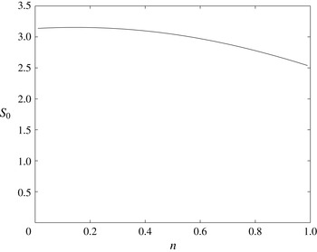
For a unitary external strain field, the strain rate
 $S_{0}$
at the vortex centre is shown as a function of the wing loading parameter
 $n$
.

In practice, the fact that
 $F(r)$
becomes unbounded for
 $r\rightarrow \infty$
poses a computational obstacle. It is resolved by defining
 $G(r)=F(r)/r^{2}$
and solving the ODE for
 $G(r)$
instead. One finds
 $G(r)\rightarrow 1$
and
 $G^{\prime }(r)\rightarrow 0$
as
 $r\rightarrow \infty$
, while a boundary condition at
 $r=0$
can be obtained easily from that for
 $F(r)$
. The constant
 $S_{0}$
is then determined using a fourth-order Runge–Kutta shooting method by integrating the equation governing
 $G(r)$
inward from a large radius and outward from
 $r=0$
, and matching both at an intermediate radius. As mentioned in the previous paragraph, the solution for
 $F(r)$
is unique. It follows that the constant
 $S_{0}$
, which measures the strain rate at the vortex centre, is unique as well. For the Moore–Saffman family of profiles introduced in § 2, the magnitude of
 $S_{0}$
depends on the value of the wing loading parameter
 $n$
. Figure 3 shows the precise nature of this dependence. An increase of the strain rate at the vortex centre can be observed for decreasing
 $n$
, from a value of
 $S_{0}\simeq 2.54$
for
 $n=0.99$
to
 $S_{0}\simeq 3.15$
for
 $n=0.20$
. Physically, this increase signifies that the unitary external strain field is felt more strongly at the vortex centre for
 $n<1$
. We will refer back to this observation at the point of interpreting our numerical results in § 4.
In order to obtain equations for a velocity–pressure perturbation
 $(\tilde{\boldsymbol{u}},\tilde{p})$
of order
 $\unicode[STIX]{x1D705}$
, the three-dimensional incompressible Navier–Stokes equations
 $$\begin{eqnarray}\displaystyle & \displaystyle \frac{\unicode[STIX]{x2202}\boldsymbol{u}}{\unicode[STIX]{x2202}t}+(\boldsymbol{u}\boldsymbol{\cdot }\unicode[STIX]{x1D735})\boldsymbol{u}=-\unicode[STIX]{x1D735}p+\frac{1}{Re}\unicode[STIX]{x1D6FB}^{2}\boldsymbol{u}, & \displaystyle\end{eqnarray}$$
 $$\begin{eqnarray}\displaystyle & \displaystyle \unicode[STIX]{x1D735}\boldsymbol{\cdot }\boldsymbol{u}=0, & \displaystyle\end{eqnarray}$$
with
 $Re$
the Reynolds number as defined in § 2.1, are linearized about the non-axisymmetric mean flow given by (3.1). The linearized governing equations are then expanded in cylindrical coordinates in a manner similar to what was done in Ash & Khorrami (Reference Ash, Khorrami and Green1995). The fluctuations to the steady state are assumed to be of the form
 $$\begin{eqnarray}\displaystyle & \boldsymbol{u}(r,\unicode[STIX]{x1D703},z,t)=\bar{\boldsymbol{u}}(r,\unicode[STIX]{x1D703})+\unicode[STIX]{x1D705}\tilde{\boldsymbol{u}}(r,\unicode[STIX]{x1D703},z,t), & \displaystyle\end{eqnarray}$$
 $$\begin{eqnarray}\displaystyle & p(r,\unicode[STIX]{x1D703},z,t)=\bar{p}(r,\unicode[STIX]{x1D703})+\unicode[STIX]{x1D705}\tilde{p}(r,\unicode[STIX]{x1D703},z,t). & \displaystyle\end{eqnarray}$$
They lead to the following equations governing the perturbation:
 $$\begin{eqnarray}\displaystyle & \displaystyle \frac{\unicode[STIX]{x2202}\tilde{\boldsymbol{u}}}{\unicode[STIX]{x2202}t}+(\tilde{\boldsymbol{u}}\boldsymbol{\cdot }\unicode[STIX]{x1D735})\bar{\boldsymbol{u}}+(\bar{\boldsymbol{u}}\boldsymbol{\cdot }\unicode[STIX]{x1D735})\tilde{\boldsymbol{u}}=-\unicode[STIX]{x1D735}\tilde{p}+\frac{1}{Re}\unicode[STIX]{x1D6FB}^{2}\tilde{\boldsymbol{u}}, & \displaystyle\end{eqnarray}$$
 $$\begin{eqnarray}\displaystyle & \unicode[STIX]{x1D735}\boldsymbol{\cdot }\tilde{\boldsymbol{u}}=0. & \displaystyle\end{eqnarray}$$
The numerical method used to solve the linearized viscous equations given by (3.10) and (3.11) is described in the following section. The domain is unbounded and the only boundary condition that is applied is the decay of the perturbation quantities at infinity. As is usually presumed (Fabre, Sipp & Jacquin Reference Fabre, Sipp and Jacquin2006; Lacaze et al.
Reference Lacaze, Ryan and Le Dizès2007), the slow viscous diffusion of the mean flow
 $\bar{\boldsymbol{u}}$
has been neglected in (3.8) and (3.9). The background flow is effectively frozen in time, so that any temporal growth can be directly attributed to the perturbation
 $\tilde{\boldsymbol{u}}$
.
3.2 Numerical method
The three-dimensional linearized Navier–Stokes equations, (3.10) and (3.11), are to be solved in cylindrical coordinates using a spectral method in space and a third-order splitting method in time. The problem of spatially discretizing the perturbation quantities
 $(\tilde{\boldsymbol{u}},\tilde{p})$
requires some thought because the physical domain is unbounded and includes the pole at
 $r=0$
. Clustering of collocation points near the coordinate singularity at the origin can restrict the size of the explicit time step. Care is taken to avoid this by choosing a suitable orthogonal basis of polynomials in the radial direction. First, the details of the spectral discretization in space are given and compared with other standard numerical approaches. Then, the time-stepping mechanism is described. Finally, the parameters of the numerical simulation are given.
Spectral methods are a popular choice due to their high accuracy and relative ease of use. The periodicity of the azimuthal variable
 $\unicode[STIX]{x1D703}$
allows a Fourier expansion. The axial variable
 $z$
does as well, provided that the axial dimension, which is inherently unbounded, is assumed to be periodic. In the radial direction, however, there are numerous families of polynomials that form suitable orthogonal bases. Our numerical routine employs mapped associated Legendre polynomials in the radial variable
 $r$
. The specifics of this spectral expansion were first formulated by Matsushima & Marcus (Reference Matsushima and Marcus1997). The orthogonal polynomials satisfy the pole condition exactly at the coordinate singularity
 $r=0$
, and their behaviour as
 $r\rightarrow \infty$
is suitable for expanding smooth functions that decay algebraically or exponentially. The associated Legendre polynomials, denoted by
 $P_{n}^{m}$
, generalize the more familiar Legendre polynomials and satisfy a similar recursion. Formulae detailing the recursion relations necessary for manipulating the polynomials
 $P_{n}^{m}$
in spectral function space can be found in Abramowitz & Stegun (Reference Abramowitz and Stegun1972).
Following Matsushima & Marcus (Reference Matsushima and Marcus1997), the radial variable
 $0\leqslant r<\infty$
is mapped to a computational variable
 $-1\leqslant \unicode[STIX]{x1D707}<1$
via the algebraic map
 $$\begin{eqnarray}\unicode[STIX]{x1D707}=\frac{r^{2}-L^{2}}{r^{2}+L^{2}},\end{eqnarray}$$
where
 $L>0$
is a map parameter that can be chosen to optimize convergence. After a considerable amount of algebra, (3.12) eliminates
 $r$
from (3.10) and (3.11) by substituting in the variable
 $\unicode[STIX]{x1D707}$
instead. All perturbation quantities are then expanded into Fourier/associated Legendre series as follows:
 $$\begin{eqnarray}\displaystyle & \displaystyle \tilde{\boldsymbol{u}}(\unicode[STIX]{x1D707},\unicode[STIX]{x1D703},z,t)=\mathop{\sum }_{k=-K}^{K}\mathop{\sum }_{m=-N}^{N}\mathop{\sum }_{n=|m|}^{N}\tilde{\boldsymbol{u}}_{k,m,n}(t)P_{n}^{m}(\unicode[STIX]{x1D707})\text{e}^{\text{i}m\unicode[STIX]{x1D703}}\text{e}^{\text{i}kz}, & \displaystyle\end{eqnarray}$$
 $$\begin{eqnarray}\displaystyle & \displaystyle \tilde{p}(\unicode[STIX]{x1D707},\unicode[STIX]{x1D703},z,t)=\mathop{\sum }_{k=-K}^{K}\mathop{\sum }_{m=-N}^{N}\mathop{\sum }_{n=|m|}^{N}\tilde{p}_{k,m,n}(t)P_{n}^{m}(\unicode[STIX]{x1D707})\text{e}^{\text{i}m\unicode[STIX]{x1D703}}\text{e}^{\text{i}kz}. & \displaystyle\end{eqnarray}$$
Here, the integers
 $N$
and
 $K$
determine the number of basis functions in the expansion. The complex coefficients
 $\tilde{\boldsymbol{u}}_{k,m,n}(t)$
and
 $\tilde{p}_{k,m,n}(t)$
are the expansion coefficients for the velocity and pressure respectively. The truncation of the radial basis in (3.13) and (3.14) is triangular in the sense that higher azimuthal wavenumbers
 $m$
are associated with fewer radial basis functions. This happens naturally as the associated Legendre polynomials satisfy
 $P_{n}^{m}(\unicode[STIX]{x1D707})=0$
for
 $n<|m|$
. Boyd (Reference Boyd2000) mentions that for spherical harmonics, a triangular truncation gives the most uniform resolution (and allows the longest time step). Although this has not been proven for the associated Legendre polynomial basis, it seems plausible that it is preferable here as well. Quadrature in the variable
 $\unicode[STIX]{x1D707}$
is performed using Gauss–Legendre collocation points. When mapped to the variable
 $r$
, half of the collocation points are guaranteed to lie between 0 and
 $L$
. In this way
 $L$
controls the resolution near the core of the vortex.
The application of associated Legendre polynomials to pseudospectral methods is relatively novel, but was shown to be successful for simulating cooperative instability in Matsushima & Marcus (Reference Matsushima and Marcus1997). More recently, Bristol et al. (Reference Bristol, Ortega, Marcus and Savaş2004) have investigated the instabilities of a pair of parallel unequal-strength vortices using the same numerical method. The spectral expansion used by these authors differs from the one used in this paper in an important way. Both Matsushima & Marcus (Reference Matsushima and Marcus1997) and Bristol et al. (Reference Bristol, Ortega, Marcus and Savaş2004) performed a toroidal and poloidal decomposition of the velocity field which eliminates the incompressibility condition (3.11) and reduces the number of unknowns. In lieu of this, we have taken adjoint complex combinations of the radial and azimuthal velocity profiles, thus simplifying the vector Laplacian. Similar considerations apply to the spectral tau-method proposed by Sakai & Redekopp (Reference Sakai and Redekopp2009). That method employs one-sided Jacobi polynomials as radial expansion functions for solving vector field equations defined in polar coordinates.
The spectral method described above has significant advantages over other numerical techniques. When compared with an approach in Cartesian coordinates using a Fourier expansion in all directions, such as the one taken by Faddy & Pullin (Reference Faddy and Pullin2005) in conjunction with a special mapping for the axial coordinate developed by Cain, Ferziger & Reynolds (Reference Cain, Ferziger and Reynolds1984), our expansion in cylindrical coordinates requires fewer basis functions to achieve a desired accuracy and allows a direct inspection of the azimuthal wavenumbers. The disadvantage is that there is no fast transform to the space of associated Legendre polynomials, thus increasing computational expense. In cylindrical coordinates, there are other polynomial bases that can be used to expand in the radial direction. Several of these are listed in Boyd (Reference Boyd2000), including Bessel functions and Chebyshev polynomials. Bessel functions have been shown to be ill-suited because of slow convergence of the expansion. Gottlieb & Orszag (Reference Gottlieb and Orszag1977) suggest using Chebyshev polynomials for a cylindrical geometry because a fast transform is available. Clustering of the grid points occurs near
 $r=0$
, however, which severely limits the time step.
Stepping in time in our numerical procedure is performed using a third-order stiffly stable splitting method devised by Karniadakis, Israeli & Orszag (Reference Karniadakis, Israeli and Orszag1991). This scheme is similar to Adams-type explicit schemes for time integration, but it has a significantly broader stability region due to the fact that the time derivative is discretized using backwards differentiation. Moreover, the convective terms in (3.10) are handled explicitly while the diffusive terms are implemented implicitly for stability reasons. The lack of a predictive equation for the evolution in time of the pressure stems from the fact that, in an optimization sense, the pressure
 $\tilde{p}$
is a Lagrange multiplier for the momentum equations associated with the divergence-free constraint. As a consequence, at every time step (of size
 $\unicode[STIX]{x0394}t$
), a Poisson equation of the form
 $$\begin{eqnarray}\unicode[STIX]{x1D6FB}^{2}\tilde{p}=\frac{1}{\unicode[STIX]{x0394}t}\unicode[STIX]{x1D735}\boldsymbol{\cdot }\tilde{\boldsymbol{u}}\end{eqnarray}$$
must be solved to determine the pressure necessary to make the velocity field
 $\tilde{\boldsymbol{u}}$
satisfy (3.11). After being initialized to random noise, the disturbance velocity field
 $\tilde{\boldsymbol{u}}$
is made divergence-free by applying a pressure gradient that is calculated in this manner. The disturbance velocity and pressure fields are then advanced in time and quickly become a combination of exponentially growing and decaying modes. In order to compute the azimuthal wavenumbers
 $m$
associated with maximum amplification for a given value of
 $k$
, we track the evolution in time of the kinetic energy
 $E(m)$
of each azimuthal Fourier mode in (3.13). The gain
 $\unicode[STIX]{x1D714}_{i}(m)$
in its energy is obtained using the following simple relation (Faddy Reference Faddy2005):
 $$\begin{eqnarray}\unicode[STIX]{x1D714}_{i}(m)=\lim _{t\rightarrow \infty }\frac{1}{2}\frac{\text{d}\ln E(m)}{\text{d}t}.\end{eqnarray}$$
Convergence of this quantity is found to be rapid in most cases. A comparison of the magnitude of
 $\unicode[STIX]{x1D714}_{i}(m)$
for all modes in the truncation admits identification of the two azimuthal wavenumbers
 $m_{1}$
and
 $m_{2}$
with the largest growth rate
 $\unicode[STIX]{x1D714}_{i}(m_{1})\simeq \unicode[STIX]{x1D714}_{i}(m_{2})$
.
The equations necessary for time-stepping the expansion coefficients
 $\tilde{\boldsymbol{u}}_{k,m,n}(t)$
and
 $\tilde{p}_{k,m,n}(t)$
given in (3.13) and (3.14), which are obtained from (3.10) and (3.15) via the splitting method formulation, have a convenient form in the sense that coefficients with different azimuthal wavenumbers
 $m$
are mostly decoupled. More specifically, both the pressure gradient and the viscous diffusion term are applied to every azimuthal wavenumber independently. There is, however, coupling between azimuthal wavenumbers (which are exactly 2 apart, i.e.
 $m-2$
,
 $m$
and
 $m+2$
) through the effect of the non-axisymmetric correction to the mean flow in the convection term of the governing equation. Nonetheless, the equations allow for an extensive parallelization of the numerical code which in turn reduces simulation runtime drastically. The method is implemented in Fortran 95 using the OpenMP interface for parallel processing.
We now discuss the range of values of the computational parameters that were used in the numerical simulations. The resolution parameter
 $L$
was found to have a significant impact on the rate of convergence and it is thus necessary to choose this parameter carefully. The optimal value of
 $L$
is found to lie between 0.5 and 6 and depends primarily on the axial wavenumber
 $k$
. The radial decay of the modes increases for decreasing
 $k$
and the collocation points have to be spread out accordingly to ensure accurate results. The time step
 $\unicode[STIX]{x0394}t$
was chosen to be of order 0.001. This size of time step was found to be sufficient to integrate the governing equation (3.10) as far as
 $t=1000$
. The asymptotic behaviour of the perturbation velocity field was thereby recovered and the dominant modes could be obtained. Axial wavenumbers were usually chosen to be between 1 and 7 with steps of 0.01, unless otherwise stated. The integer
 $N$
in (3.13) and (3.14) was chosen to be of the order of 60, although accurate results could already be obtained for
 $N$
as low as
 $25$
. Numerically,
 $N$
determines the number of azimuthal (and radial) wavenumbers. For example,
 $N=25$
corresponds to 51 Fourier modes in the azimuthal direction. When
 $N$
is increased, which corresponds to increasing the number of azimuthal and radial modes, the time step
 $\unicode[STIX]{x0394}t$
is decreased. Specifically,
 $\unicode[STIX]{x0394}t$
is taken to be inversely proportional to
 $N$
.
3.3 Numerical convergence and code verification
Several checks were performed in order to assure that the numerical routine functions as desired. In this section, we compare some of our results with previously published data and obtain excellent agreement. In addition, we present convergence analyses of the numerical method in order to show that in most cases a very low number of spectral modes is needed to get an accurate estimate of the instability growth rate. Results are first presented for instabilities in the absence of strain. After this, a strain field is introduced and elliptical instability growth rates are verified. Finally, the effect of the physical parameter
 $a$
, introduced in (2.7), on the numerical results is illustrated.
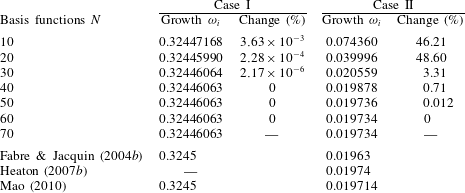
To begin with, we reproduce several published results for modes of instability of the Batchelor vortex in the absence of strain (
 $\unicode[STIX]{x1D700}=0$
). In table 1, comparisons are presented for two unstable modes: an inviscid mode in the presence of viscosity (case I) and a viscous centre mode (case II). For case I, the governing equations were integrated to
 $t=300$
. For case II, due to the smaller growth rate of the instability, we integrated until
 $t=800$
. As is well known, the growth rate of centre modes is at least an order of magnitude smaller than that of inviscid modes. In both cases, convergence is observed with an increase in the number of basis functions. Looking at case I, the growth rate of the instability is already determined quite accurately for
 $N=10$
. Little gain in accuracy is perceived in runs with progressively higher values of
 $N$
. We find the growth rate to be
 $\unicode[STIX]{x1D714}_{i}=0.32446063$
, all digits being significant. Excellent agreement with the numerical results of Fabre & Jacquin (Reference Fabre and Jacquin2004b
) and Mao (Reference Mao2010) is obtained. Case II is a viscous centre mode, which is a mode of instability with a perturbation field concentrated in the vortex centre and which occurs only in the presence of viscosity. Convergence is found to be somewhat slower than for case I, which is expected due to the nature of its perturbation velocity field and small growth rate. Viscous centre modes are not expected to participate in the elliptical instability mechanism; case II was examined only to verify our code. The numerical routine yields a growth rate of
 $\unicode[STIX]{x1D714}_{i}=0.019734$
, all digits being significant. Many recent computations have been made for this type of mode, for example by Fabre & Jacquin (Reference Fabre and Jacquin2004b
), Heaton (Reference Heaton2007b
) and Mao (Reference Mao2010). Table 1 demonstrates that our numerical result agrees well with all three of these investigations.
Code verification against published results for the Batchelor vortex for two cases of vortex instability. Case I is an unstable inviscid mode in the presence of viscosity for
 $Re=1000$
,
 $q=0.761$
,
 $m=-3$
and
 $k=1.659$
. Case II corresponds to an unstable viscous centre mode for
 $Re=14000$
,
 $q=2$
,
 $m=-1$
and
 $k=0.268$
. The change column presents the relative error (in per cent) between the growth rate in every row and the following one.

Next, we look at the Batchelor vortex subject to a strain field of magnitude
 $\unicode[STIX]{x1D700}=0.0625$
. Figure 4 shows numerical convergence results representative of those for all simulations of elliptical instability performed in this study. The results displayed in this figure were obtained for a specific set of flow parameter values and
 $n=0.95$
, a value of the wing loading parameter for which the mean flow profiles closely resemble those of the Batchelor vortex. We refer to this set-up as case III. For the flow parameters chosen, a resonance occurs between the strain field and the pair of azimuthal wavenumbers
 $(m_{1},m_{2})=(-2,0)$
. For each sample point on the curve, a random initial perturbation velocity field was advanced in time. As was mentioned in § 3.2, the perturbation growth rate is extracted by running the simulation for a sufficiently long time. To ensure accurate results, the equations for case III presented here were solved up to time
 $t=400$
. The most unstable perturbation component quickly develops exponential growth, which allows us to extract a numerical growth rate. The growth rate
 $\unicode[STIX]{x1D714}_{i}$
of the instability was found to be close to 0.0851.
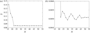
(a) The convergence of the growth rate
 $\unicode[STIX]{x1D714}_{i}$
with an increasing number of modes
 $N$
for case III. The following parameters are fixed:
 $n=0.95$
(approximately Batchelor),
 $\unicode[STIX]{x1D700}=0.0625$
,
 $W_{0}=0.482$
,
 $Re=3180$
and
 $k=1.88$
. The resulting elliptical instability is characterized by a resonance between the strain field and the azimuthal wavenumbers
 $(m_{1},m_{2})=(-2,0)$
. In (b), the region near the asymptotic value of
 $\unicode[STIX]{x1D714}_{i}$
has been magnified. In both plots, the dots represent sample points.

The present results compare favourably with the single previous investigation of this case of which we are aware. The numerical result given by Lacaze et al. (Reference Lacaze, Ryan and Le Dizès2007) is
 $\unicode[STIX]{x1D714}_{i}/\unicode[STIX]{x1D700}\simeq 1.23$
, which corresponds to
 $\unicode[STIX]{x1D714}_{i}=0.0769$
. The same authors find a theoretical prediction equal to
 $\unicode[STIX]{x1D714}_{i}/\unicode[STIX]{x1D700}\simeq 1.32$
, and this corresponds to
 $\unicode[STIX]{x1D714}_{i}\simeq 0.0825$
. With regard to convergence, figure 4(a) shows that our computation rapidly approaches an asymptotic value between
 $N=16$
and
 $N=22$
. For higher values of
 $N$
, a slight oscillation in
 $\unicode[STIX]{x1D714}_{i}$
is visible, but its amplitude is small and decreasing. A magnified version of the same curve is presented in figure 4(b), and it shows the convergence behaviour more clearly. The oscillation amplitude can be seen to diminish rapidly to less than
 $10^{-4}$
for
 $N\approx 50$
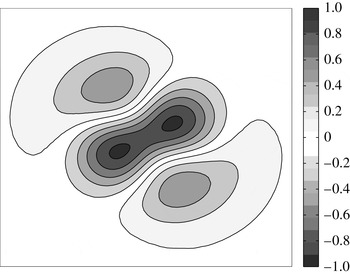
. This provides clear evidence of the correct functioning of our numerical scheme. A look at figure 5 confirms this conclusion. This figure displays the perturbation vorticity field associated with the mode of resonance in case III. The contours shown in this figure can be compared with those in figure 15(a) from Lacaze et al. (Reference Lacaze, Ryan and Le Dizès2007); the modal structures are seen to resemble one another closely.
The perturbation vorticity field for the unstable mode named case III. The elliptical instability structure is visible as a combination of modes with azimuthal wavenumbers
 $m_{1}=-2$
and
 $m_{2}=0$
. The contours, which are isovorticity lines, are spaced 0.2 apart. The zero-vorticity contour is not displayed. Two poles of negative vorticity (with a minimum value of
 $-1$
) and two poles of positive vorticity (with a maximum value of approximately 0.6) exist.

To conclude this section, we briefly revisit the discussion in § 2.2 about the dependence of our numerical results on
 $a$
, which is the non-dimensional parameter that dictates the point of transition from the Moore–Saffman profiles, in the inner region of the vortex, to the inviscid outer solution described by (2.8). Throughout our calculations we have observed a negligible dependence on
 $a$
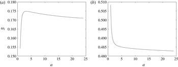
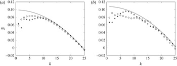
when its value is sufficiently large. To illustrate this, figure 6 shows the growth rates
 $\unicode[STIX]{x1D714}_{i}$
as a function of
 $a$
for two trial cases (both modes of elliptical instability). The physical parameters for the two plots in this figure are quite different, yet we observe the same behaviour in both: the growth rates change somewhat for
 $a\lesssim 3$
and converge when
 $a$
is greater than that value. The fact that the results remain mostly invariant under a change of
 $a$
is a subtle but direct consequence of our choice in § 2.1 to normalize the core circulation instead of the far-field circulation. We used
 $a=5$
to generate the numerical results in § 4, unless stated otherwise.
The dependence of the growth rate
 $\unicode[STIX]{x1D714}_{i}$
on the core radius parameter
 $a$
is displayed for elliptical modes of instability for (a)
 $\unicode[STIX]{x1D700}=0.0625$
,
 $W_{0}=0.482$
,
 $Re=3180$
,
 $k=1.88$
and
 $n=0.50$
and (b)
 $\unicode[STIX]{x1D700}=0.0625$
,
 $W_{0}=0.15$
,
 $Re=20000$
,
 $k=4.5$
and
 $n=0.70$
.

4 Numerical results
We start this section by presenting findings for the elliptical instability in the linearly stable and unstable regimes of the base flow. For the sake of clarity, we will refer to the linear instability of a single vortex, i.e. any modes of instability that are not associated with a cooperative mechanism, as ‘swirling flow instability’. The influence of the Moore–Saffman wing loading parameter
 $n$
on the growth rate
 $\unicode[STIX]{x1D714}_{i}$
of the elliptical instability is our primary point of interest. We have obtained results for values of
 $n$
between 0.20 and 0.99. Next, disturbances with a very short axial wavelength are considered, and the effect of viscosity and the strain rate on the modes of elliptical instability is discussed. The impact of the axial flow parameter
 $W_{0}$
on the growth rates of the instability is examined after that. To conclude, we visualize the structure of the perturbation vorticity field for a number of elliptical modes of instability.
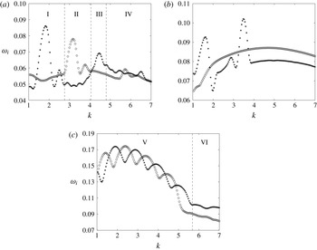
Figure 7 displays the dependence of the growth rates of the elliptical instability on the axial wavenumber
 $k$
for three values of
 $n$
. Results for
 $n=0.95$
are displayed in figure 7(a). Although the mean velocity profiles for this value of
 $n$
closely approximate those of the Batchelor vortex in the near field, the asymptotic behaviour for large
 $r$
is not the same. For instance, the axial mean velocity
 $W(r)$
decays algebraically and not exponentially for
 $r\rightarrow \infty$
. The curves in figure 7(a) consist of a series of parabolic arcs in narrow bands which correspond to different resonant pairs of azimuthal wavenumbers. We find the three most unstable axial wavenumbers to be
 $k\simeq 1.84$
,
 $k\simeq 3.19$
and
 $k\simeq 4.48$
. The corresponding growth rates are
 $\unicode[STIX]{x1D714}_{i}\simeq 0.0861$
,
 $\unicode[STIX]{x1D714}_{i}\simeq 0.0782$
and
 $\unicode[STIX]{x1D714}_{i}\simeq 0.0691$
respectively. All three modes were found by previous investigations (see Lacaze et al. (Reference Lacaze, Ryan and Le Dizès2007), discussed further below) to be principal modes; they are associated with a resonance between modes having the same radial (nodal) structure. Separating them are branches of less unstable modes, at approximately
 $k\simeq 2.50$
and
 $k\simeq 3.76$
, which are composed of non-principal modes. The present numerical study can determine the azimuthal and radial structure of elliptical modes of instability, but it cannot ascertain whether a mode is principal or not. Analytical estimates are necessary to do that.
The growth rate
 $\unicode[STIX]{x1D714}_{i}$
is presented as a function of the axial wavenumber
 $k$
for the Moore–Saffman vortex with (a)
 $n=0.95$
, (b)
 $n=0.70$
and (c)
 $n=0.50$
. The flow parameters are maintained at
 $\unicode[STIX]{x1D700}=0.0625$
,
 $W_{0}=0.482$
and
 $Re=3180$
throughout. Resonances of odd and even azimuthal wavenumbers are represented by star and circle symbols respectively. The vertical dotted lines delimit certain regions of interest. Each region is labelled by a Roman numeral and treated further in the text.

The most amplified resonant pair of azimuthal wavenumbers
 $(m_{1},m_{2})$
changes with
 $k$
. The Roman numerals I–IV mark several regions in figure 7(a); each region constitutes a different mode of elliptical instability. In region I, the dominant odd pair is
 $(m_{1},m_{2})=(-1,1)$
and the dominant even pair is
 $(-2,0)$
. It is clear from the figure that neither resonance is the fastest growing throughout this region. The growth rate of the pair
 $(-2,0)$
peaks twice, at locations given in the previous paragraph. For higher values of
 $k$
, several interchanges take place between odd and even resonant pairs, from
 $(-3,-1)$
in region II to
 $(-4,-2)$
in region III, as the most rapidly growing mode of elliptical instability. For even shorter axial wavelengths, i.e. region IV where
 $k\gtrsim 4.79$
, numerous odd and even resonances become dominant in rapid succession. Our calculations yield the modes
 $(-2,0)$
,
 $(-4,-2)$
and
 $(-5,-3)$
there.
In comparison, for the same parameter configuration, Lacaze et al. (Reference Lacaze, Ryan and Le Dizès2007) present the resonant modes in figure 14 and table 1 of their paper, employing
 $\unicode[STIX]{x1D70E}=\unicode[STIX]{x1D714}_{i}/\unicode[STIX]{x1D700}$
to express the growth rate. It is the sole reference of which we are aware that contains detailed information regarding growth rates for the cooperative instability of counter-rotating Batchelor vortices. The present findings are in good agreement with the results shown there, particularly the locations of the maxima of the growth rate. There is a slight departure in the values of the growth rates themselves. The deviation increases when
 $k$
is increased. It is worthwhile to briefly point out three dissimilarities between the current study and two interconnected prior investigations, namely Lacaze et al. (Reference Lacaze, Ryan and Le Dizès2007) and Roy et al. (Reference Roy, Schaeffer, Le Dizès and Thompson2008), although the latter deals mostly with co-rotating vortex pairs. A first difference resides in the fact that we model the effect of the strain field as a first-order correction to a single vortex, and use this velocity field to linearize the governing equations. Second, since the simulation is performed in cylindrical coordinates, it is able to identify, independently for even and odd azimuthal wavenumbers, two potentially unstable elliptical modes per axial wavenumber
 $k$
. A third difference, again related to the numerical method taking advantage of the cylindrical geometry, is that we are not obliged to look at the perturbation vorticity field to identify the azimuthal structure of the unstable mode. The first point mentioned here implies that, as is common in stability studies, the strained mean velocity field satisfies the Euler equations at first order of the strain field, but not the Navier–Stokes equations. The impact of this fact on the results is expected to become more significant as
 $k$
increases.
The other panels in figure 7 present numerical results for the elliptical instability of the strained Moore–Saffman vortex for two other wing loading distributions. Figure 7(b) demonstrates how the growth rates of the instability vary with
 $k$
for
 $n=0.70$
. The curves in this figure differ considerably from those in figure 7(a) in two ways. First, the growth rates are on average significantly larger than those for
 $n=0.95$
. Depending on the value of
 $k$
, the difference may be greater than 20 %. Second, the narrow bands of unstable axial wavenumbers are exchanged for a continuum of unstable wavenumbers when
 $k$
is sufficiently large. In particular, the unstable modes consisting of even azimuthal wavenumbers in this figure are situated on a continuous branch in the shape of a wide arc. This phenomenon, which we attribute to the presence of a continuum of unstable modes with short wavelength, is discussed in some detail in the section on the ultra-short-wave cooperative instability (Chap. 12) of the book by Saffman (Reference Saffman1992). The existence of a large growth envelope has also been reported by Roy et al. (Reference Roy, Schaeffer, Le Dizès and Thompson2008), specifically in figure 9 of their paper, where it is illustrated for the case of a pair of co-rotating vortices with no axial flow, and in their figure 6, where axial flow is present. Returning to figure 7(b), the most amplified modes for most of the domain are resonances between Kelvin modes with odd azimuthal wavenumbers. Two bands of instability of even wavenumbers, centred at
 $k\simeq 1.61$
and
 $k\simeq 3.49$
, can be observed. Resonant parabolae only persist in the vicinity of these two values of the axial wavenumber. The peak amplification rates in these two bands are in excess of
 $\unicode[STIX]{x1D714}_{i}=0.09$
and
 $\unicode[STIX]{x1D714}_{i}=0.10$
respectively. There are no other locations where even pairs of azimuthal wavenumbers are the most amplified elliptical disturbances. It should be noticed that no regions have been marked in this figure; for the complete spectrum of axial wavenumbers, we find the resonant odd and even wavenumbers to be
 $(m_{1},m_{2})=(-1,1)$
and
 $(-2,0)$
respectively.
The growth rate
 $\unicode[STIX]{x1D714}_{i}$
is displayed as a function of the axial wavenumber
 $k$
for fixed flow parameters
 $\unicode[STIX]{x1D700}=0.0625$
,
 $W_{0}=0.482$
and
 $Re=3180$
, for the Moore–Saffman vortex with (a)
 $n=0.50$
and (b)
 $n=0.60$
. Resonances of odd and even azimuthal wavenumbers are represented by circle and star symbols respectively. The solid lines display growth rates of inviscid modes of swirling flow instability (i.e. for
 $\unicode[STIX]{x1D700}=0$
and
 $\unicode[STIX]{x1D708}=0$
); each branch corresponds to a different azimuthal wavenumber
 $m$
, as indicated.

The situation for
 $n=0.50$
, displayed in figure 7(c), reveals a more complex structure. Before considering region V in detail, we briefly discuss the information in region VI, where
 $k\gtrsim 5.68$
. We detect cooperative instability for these short axial wavelengths, the dominant pair of wavenumbers always being
 $m_{1}=-4$
and
 $m_{2}=-2$
. While the growth rates of these modes are low in this figure, it becomes clear after a comparison with figure 7(a) that they are larger than that of the most amplified mode of elliptical instability of the Batchelor vortex. Turning now to region V, we start by pointing out that the series of short parabolae, alternating between odd and even pairs, is due to swirling flow instability. This can be understood by noting the axial flow strength chosen in this figure; it is maintained at the relatively high value of
 $W_{0}=0.482$
, which permits linear instability of the Moore–Saffman base flow, as was indicated in § 2.3. In order to interpret the elevated rates of growth in figure 7(c) from what was discussed in that section, it is important to keep in mind that although the modes with azimuthal wavenumber
 $m=-1$
define the region of instability for a single unstrained vortex, the growth rate of higher modes of instability is much greater, and, furthermore, that these modes for
 $m\rightarrow \infty$
only become damped due to viscosity.
A broader look at the findings in figure 7 suggests the presence of three types of instability in the results of our numerical simulation. A first type is the swirling flow instability; it is discernible by the closely spaced arcs in region V. Next, in figures 7(a) and 7(b), we observe modes of elliptical instability whose growth rates are organized in narrow parabolic arcs. A third type consists of modes of elliptical instability belonging to a continuum. The wide arcs associated with this continuum are most clearly observable in 7(b).
Several observations specifically concern the manifestation of both swirling flow and elliptical instability in the vortex. For clarity, a magnified view of the results in figure 7(c) for a selected range of
 $k$
is provided in figure 8(a). Together with the findings of our simulation of the strained vortex, we display several solid lines showing growth rates of inviscid modes of swirling flow instability; that is to say, unstable modes of a single vortex in the absence of viscosity. It is clear from looking at the figure that the circle and star symbols follow the branches for
 $m=-5$
,
 $m=-6$
and
 $m=-7$
accurately. The growth in the strained vortex for these axial wavenumbers is therefore due to the amplification of single azimuthal Fourier components of the initial perturbation. It can be seen that the growth rates for
 $\unicode[STIX]{x1D700}=0.0625$
are slightly below those of the unstrained vortex. This is because of the absence of viscosity in the calculation of the latter. In addition, the strain field is affecting the growth rates of the modes of instability of the unstrained vortex, further comments on which are provided at the end of this section.
More importantly, the apparent lack of additional growth due to interactions between azimuthal wavenumbers in region V seems to imply that elliptical instability may not occur in this region of intense swirling flow instability or that it may not be detectable. As shown in figure 8(b), for
 $n=0.60$
, one can have both instabilities coexisting. This figure exhibits features similar to those of figure 8(a), namely swirling flow instability with odd
 $m$
interspersed with even
 $m$
, but it also includes a resonant parabola at
 $k\simeq 3.54$
. For this axial wavenumber, an unstable interaction of
 $m_{1}=-2$
and
 $m_{2}=0$
exists with peak amplification rate
 $\unicode[STIX]{x1D714}_{i}\simeq 0.121$
. Moreover, even though numerous swirling flow instabilities take place in this figure, we find the elliptical mode for the aforementioned axial wavenumber to be the most amplified disturbance for
 $n=0.60$
and any
 $k>1$
.
Contour plots of the maximum growth rate
 $\unicode[STIX]{x1D714}_{i}$
for every value of the axial wavenumber
 $k$
and wing loading parameter
 $n$
are presented for
 $W_{0}=0.482$
. The other flow parameters are
 $\unicode[STIX]{x1D700}=0.0625$
and
 $Re=3180$
. At every point of the
 $(k,n)$
-plane, the rate of growth in time of a random initial perturbation is displayed. The contours are curves of constant growth rate. They are spaced 0.01 apart and the highest contour is
 $\unicode[STIX]{x1D714}_{i}=0.18$
.

Figure 9 presents the growth rate of the most amplified cooperative disturbance for every point in the
 $(k,n)$
-plane. This figure gives an overview of the findings we have discussed so far in this section since the parameters
 $\unicode[STIX]{x1D700}=0.0625$
and
 $Re=3180$
are unchanged from figures 7 and 8. For every value of
 $k$
and
 $n$
, the most unstable mode is considered irrespective of whether it is a resonance between even or odd azimuthal wavenumbers, or a mode of swirling flow instability. We point out four main features of this figure. A first prominent aspect is the distinctive arcs that are visible in the contours for
 $1\lesssim k\lesssim 4$
and
 $0.40\lesssim n\lesssim 0.60$
. They were deemed earlier in this section to be a consequence of the linearly unstable modes of a single Moore–Saffman vortex that occur in this region of parameter space (see figure 8). Second, we observe multiple elliptical modes of instability that can be tracked downward from
 $n=0.95$
, most notably the resonance
 $(m_{1},m_{2})=(-2,0)$
at
 $k\simeq 1.88$
, until their disappearance. Other resonant couplings emerge for
 $n<0.95$
, for instance near
 $n\simeq 0.60$
and
 $k\simeq 3.54$
, and several modes with high amplification rates are encountered near
 $n\simeq 0.20$
. Next, one can note the appearance of a continuum of modes for
 $0.60\lesssim n\lesssim 0.90$
when
 $k$
is relatively small. The growth rates of the unstable modes in this continuum are situated on a wide arc rather than on narrow parabolic branches, indicating weak dependence of their growth rate on the axial wavenumber. For values of
 $n$
outside this interval, the continuum appears only for unstable waves with a very short axial wavelength. Finally, we point out that the growth rates for the Moore–Saffman vortex with
 $n<0.95$
exceed those for both
 $n=0.95$
and the Batchelor vortex. Maximum amplification can be seen to occur for
 $n\simeq 0.44$
, even though, as pointed out earlier, this growth is due to swirling flow instability.
Contour plots of the maximum growth rate
 $\unicode[STIX]{x1D714}_{i}$
for every value of the axial wavenumber
 $k$
and wing loading parameter
 $n$
are presented for
 $W_{0}=0.2494$
. The other flow parameters are
 $\unicode[STIX]{x1D700}=0.0625$
and
 $Re=3180$
. At every point of the
 $(k,n)$
-plane, the rate of growth in time of a random initial perturbation is displayed. The contours are curves of constant growth rate. They are spaced 0.01 apart and the highest contour is
 $\unicode[STIX]{x1D714}_{i}=0.13$
.

In figure 10, the calculations from figure 9 are repeated for a reduced axial flow parameter value of
 $W_{0}=0.2494$
. Although this is narrowly outside the linearly stable regime described in § 2.3, any existing unstable modes will grow very slowly in time and are therefore not expected to interfere in the elliptical instability process. No obvious signs of swirling flow instability can be discerned in figure 10. Furthermore, our examination of the dominant resonant configurations for the parameter space considered in this figure has confirmed that all disturbance growth is linked to modes of elliptical instability. Notwithstanding the absence of swirling flow instability, this figure resembles figure 9 in several ways: the presence of a continuum of modes, the destabilization exhibited when
 $n$
is decreased and the recovery of
 $n\simeq 0.44$
as being a particularly unstable value of the wing loading parameter. One can further note the difference in structure of the contour lines between the lower and upper halves of this figure; there are strongly amplified modes for
 $n\lesssim 0.44$
that do not appear to be organized in bands. Finally, the growth rates for
 $W_{0}=0.2494$
are smaller than those for
 $W_{0}=0.482$
in figure 9, consistent with previous investigations that have found the role of an axial flow to be destabilizing.
Figures 9 and 10 illustrate the significant influence of the wing loading parameter
 $n$
on the elliptical instability. We now comment on the reasons for this and relate our findings to those in the literature. In light of previous investigations (namely Lacaze et al.
Reference Lacaze, Birbaud and Le Dizès2005, Reference Lacaze, Ryan and Le Dizès2007; Roy et al.
Reference Roy, Schaeffer, Le Dizès and Thompson2008), which have included the effect of axial flow, the complicated dynamics we have observed to be associated with a change in
 $n$
may be understood to stem from the fact that variations of this parameter profoundly change the shape of the axial mean velocity
 $W(r)$
(see figure 1
b). However, the particular decay imposed by (2.6) on the velocity components already plays an important role. Fabre & Jacquin (Reference Fabre and Jacquin2004a
) studied the short-wave cooperative instability of a vortex model with an azimuthal mean velocity component that decays algebraically in an intermediate region, somewhat similar to the model considered here but with no axial flow. They found the stability characteristics to transition in the range
 $0.40<n<0.50$
from elliptical instability of the internal core, for
 $0.50<n<1$
, to what they describe as an instability of the intermediate zone, for
 $0<n<0.40$
. In the transition range, they observed large instability bands that under certain circumstances may coalesce into a broadband spectrum. As a last element, we refer back to figure 3 to point out that the strain rate at the vortex centre increases slightly when
 $n$
is decreased from
 $n\simeq 1$
. This may explain, at least in part, the larger amplification rates of elliptical instability that we observe for the Moore–Saffman vortex profiles.
Figure 11 displays detailed results for the large-axial-wavenumber behaviour of the instability growth rates for the Moore–Saffman vortex with
 $n=0.80$
and
 $n=0.50$
. The vortex is stable to the swirling flow instability for the axial flow strength
 $W_{0}=0.15$
considered in this figure (see § 2.3). The instabilities for large values of
 $k$
are to an increasing extent damped by viscosity as
 $Re$
increases. Landman & Saffman (Reference Landman and Saffman1987) found an estimate for the time-averaged viscous decay rate, which they denoted by
 $\unicode[STIX]{x1D70E}_{V}$
. For a small strain rate
 $0<\unicode[STIX]{x1D700}\ll 1$
, their expression is bounded from below by
 $$\begin{eqnarray}-\frac{k^{2}}{Re}\left(1+\frac{\unicode[STIX]{x1D700}}{\unicode[STIX]{x1D6FE}}\right),\end{eqnarray}$$
where
 $\unicode[STIX]{x1D6FE}$
is a positive constant equal to half of the constant axial vorticity at the vortex centre. The intuitive formula
 $-k^{2}/Re$
for the viscous damping is recovered for the unstrained case (
 $\unicode[STIX]{x1D700}=0$
). The approximation given in (4.1) is represented by a solid line in figure 11. The line correlates well with the data in both plots of this figure. It should be noted that the predicted viscous decay rate is not the same for figures 11(a) and 11(b) since the core axial vorticity of the base mean flow depends on
 $n$
. While the value for the Batchelor vortex is
 $\unicode[STIX]{x1D6FE}=1$
, the corresponding quantity for the Moore–Saffman profiles is smaller, due to the scaling in (2.4) of the functions
 $V_{n}$
displayed in figure 1(a). The lower core axial vorticity leads to a diminished value of
 $\unicode[STIX]{x1D6FE}=0.8595$
for
 $n=0.80$
in figure 11(a) and
 $\unicode[STIX]{x1D6FE}=0.6420$
for
 $n=0.50$
in figure 11(b). As a consequence, an increased amount of viscous damping can be expected for any value of
 $n$
for the Moore–Saffman mean flow profiles. This reasoning does not take into account the presence of an axial flow. Notwithstanding the stronger damping by viscosity, the amplification rates in figure 11(b) are seen to be greater than those in figure 11(a) by up to 20 % depending on the value of
 $k$
. It is further apparent that no instability persists past a critical value
 $k_{c}$
of the axial wavenumber. We have determined the precise point of viscous cutoff for a limited number of parameter sets. In figure 11(a), the axial wavenumber at which cutoff occurs is
 $k_{c}\simeq 24.29$
. In figure 11(b), for
 $n=0.50$
, the viscous cutoff point is situated at
 $k_{c}\simeq 25.41$
, which represents a slight increase from the case
 $n=0.80$
. We likewise computed the threshold for the Batchelor vortex for the same
 $\unicode[STIX]{x1D700}$
,
 $W_{0}$
and
 $Re$
as in the figure; at
 $k_{c}\simeq 21.96$
, we found it to be smaller than the aforementioned values for the Moore–Saffman vortex.
The growth rate
 $\unicode[STIX]{x1D714}_{i}$
as a function of the axial wavenumber
 $k$
for fixed flow parameters
 $\unicode[STIX]{x1D700}=0.0625$
,
 $W_{0}=0.15$
and
 $Re=6000$
, for the Moore–Saffman vortex with (a)
 $n=0.80$
and (b)
 $n=0.50$
. The solid line displays the damping due to viscosity. The viscous decay rate is estimated using the expression
 $-(k^{2}/Re)(1+\unicode[STIX]{x1D700}/\unicode[STIX]{x1D6FE})$
. Resonances of odd and even azimuthal wavenumbers are represented by circle and star symbols respectively.

Figure 12 sheds light on the dependence of the instability growth rates on the Reynolds number. Again, it regards a set of parameters for which a single Moore–Saffman vortex is linearly stable for all values of
 $n$
, specifically
 $W_{0}=0.15$
, so that any growing disturbance is attributable to elliptical instability. The growth rates of the most amplified odd and even resonant couplings are shown separately, in figures 12(a) and 12(b) respectively. One should note the logarithmic scale of the vertical axis in both graphs. In order to make it easier to distinguish the regions of dominant odd and even resonant wavenumbers, thick lines overlie both plots in the figure. They can be seen to partition the parameter space into four large vertical zones and a smaller circular one. From left to right, these vertical zones consist of unstable modes composed of the following pairs of azimuthal wavenumbers: odd, even, odd and even. In the circular region, the even resonances are the most amplified instabilities. One main observation from this figure is that the presence of viscosity reduces the growth rates from values greater than
 $\unicode[STIX]{x1D714}_{i}=0.20$
for
 $Re=10^{9}$
to less than
 $\unicode[STIX]{x1D714}_{i}=0.10$
for
 $Re=10^{3.5}\simeq 3162$
. These results agree with the effect of viscosity on the elliptical instability as outlined in § 1. We emphasize here that the instability mechanism as described by Moore & Saffman (Reference Moore and Saffman1975) is essentially inviscid. The inviscid limit is approached at the top of figure 12, where several narrow bands containing resonant parabolae are visible. These resonances are centred at
 $k\simeq 1.53$
,
 $k\simeq 2.69$
,
 $k\simeq 3.95$
and
 $k\simeq 6.44$
with corresponding growth rates of
 $\unicode[STIX]{x1D714}_{i}=0.251$
,
 $\unicode[STIX]{x1D714}_{i}\simeq 0.266$
,
 $\unicode[STIX]{x1D714}_{i}\simeq 0.250$
and
 $\unicode[STIX]{x1D714}_{i}\simeq 0.217$
. The bands only arise above
 $Re\simeq 10^{4.5}$
; below this value, no resonant parabolae can be discerned in this figure.
Contour plots of the growth rate
 $\unicode[STIX]{x1D714}_{i}$
as a function of the axial wavenumber
 $k$
and the Reynolds number
 $Re$
for
 $\unicode[STIX]{x1D700}=0.0625$
,
 $W_{0}=0.15$
and
 $n=0.50$
. At every point in the
 $(k,\log (Re))$
-plane, the growth rate of the most amplified elliptical disturbance for (a) odd and (b) even wavenumbers is shown. In both plots, the contours (drawn as thin lines and distinguished by shades of grey) are curves of constant growth rate and are spaced 0.02 apart with the highest contour being
 $\unicode[STIX]{x1D714}_{i}=0.25$
. The thick curves show where the growth rates in (a) and (b) are equal and hence separate the regions of dominant odd and even resonant wavenumbers.

In order to address another important question, namely the effect of the axial flow parameter
 $W_{0}$
on the instability growth rates and the dominant resonant pair, we have employed our numerical routine for a wide range of points in the
 $(k,W_{0})$
-plane. The dominant resonant configuration that exists for a specific parameter set is determined by calculating the energy of each azimuthal Fourier mode of the perturbation velocity fields (see § 3.2 for details). Results for several values of
 $n$
are shown infigures 13–15.
Growth rate and resonant configuration for the most unstable mode for a wide range of values of the axial wavenumber
 $k$
and axial flow parameter
 $W_{0}$
. The wing loading parameter equals
 $n=0.95$
. The other parameters remain fixed at
 $\unicode[STIX]{x1D700}=0.0625$
and
 $Re=3180$
. In (a), the contours are curves of constant growth rate and they are spaced 0.005 apart with
 $\unicode[STIX]{x1D714}_{i}=0.066$
being the lowest contour that is displayed. Several contours have been labelled for clarity. A corresponding diagram with the most unstable resonant pairs is displayed in (b).

The topography of the contours for
 $n=0.95$
, in figure 13, demonstrates the major impact of
 $W_{0}$
on both the most unstable resonant pairs and their growth rates. Elliptical resonances, which are seen as islands in both plots of this figure, appear and disappear when the value of
 $W_{0}$
is increased to 0.525. The three resonant pairs that are apparent for
 $W_{0}=0$
, all of which correspond to resonances
 $(m_{1},m_{2})=(-1,1)$
and have undergone close examination in the literature on the Lamb–Oseen vortex, already become damped for a small amount of axial mean flow. Three resonances related to the interaction between
 $m_{1}=-2$
and
 $m_{2}=0$
develop at approximately
 $W_{0}=0.15$
in the
 $(k,W_{0})$
-plane. Only the island at
 $k\simeq 1.8$
persists for a large amount of axial flow; it is the most unstable resonance for
 $n=0.95$
, as it is for the Batchelor vortex. When the magnitude of the axial flow is increased further, to
 $W_{0}=0.525$
, higher modes of instability are manifested. Specifically, two resonant parabolae associated with
 $(m_{1},m_{2})=(-3,-1)$
are located at
 $k\simeq 3.21$
and
 $k\simeq 3.75$
. For higher axial wavenumbers, we recover two more islands belonging to the resonant pair
 $(m_{1},m_{2})=(-4,-2)$
and one belonging to
 $(m_{1},m_{2})=(-5,-3)$
.
The same as figure 13 but for
 $n=0.70$
. The contours in (a) are spaced 0.01 apart with
 $\unicode[STIX]{x1D714}_{i}=0.07$
being the lowest contour that is displayed.

The same as figure 13 but for
 $n=0.50$
. The contours in (a) are spaced
 $0.01$
apart with
 $\unicode[STIX]{x1D714}_{i}=0.08$
being the lowest contour that is displayed.

In figure 14, which presents data for
 $n=0.70$
, a very different picture emerges. Figure 14(a) shows the growth rates of the most unstable elliptical modes. The continuum of modes is observable by the wide arcs on the right, while a fine structure in the contours is conspicuous for
 $k\lesssim 2.2$
. The growth rates decrease when the axial flow parameter is increased from
 $W_{0}=0$
, with a minimum being attained at
 $W_{0}\simeq 0.30$
. When more axial velocity is included in the mean flow model, up to
 $W_{0}=0.525$
at which point the computation was halted, the growth rates can be seen to increase once again. Overall, however, the amplification rates are significantly higher than those for the Batchelor vortex. The ridge at the top of the figure corresponds to a strongly amplified mode of elliptical instability. The diagram of the resonant configurations, in figure 14(b), reveals that many of the most rapidly growing modes correspond to a resonance of
 $m_{1}=-1$
and
 $m_{2}=1$
. The resonance
 $(-2,0)$
is the most amplified for
 $W_{0}\gtrsim 0.37$
. Aside from a very small region where
 $m_{1}=-3$
and
 $m_{2}=-1$
are resonating, no higher modes of instability are dominant for
 $1\leqslant k\leqslant 7$
and
 $0\leqslant W_{0}\leqslant 0.525$
. This is somewhat surprising given the results in figure 13 for
 $n=0.95$
, and those reported for the Batchelor vortex by Lacaze et al. (Reference Lacaze, Ryan and Le Dizès2007). The findings in figure 14(b) are more reminiscent of the ones presented by Lacaze et al. (Reference Lacaze, Birbaud and Le Dizès2005) for a Rankine vortex with constant axial flow. The results in their figure 6, which displays a partition of the
 $(W_{0},\unicode[STIX]{x1D700}Re)$
-plane according to which a dominant resonant pair occurs, show some similarity to ours, provided that we set
 $\unicode[STIX]{x1D700}=0.0625$
and
 $Re=3180$
. It should be noted that only a resonance of
 $m=0$
and
 $|m|=2$
was observed by Roy et al. (Reference Roy, Leweke, Thompson and Hourigan2011) in an experimental set-up of a pair of counter-rotating vortices with axial core flow. To conclude, we point out that the Moore–Saffman vortex with
 $n=0.70$
becomes increasingly linearly unstable when
 $W_{0}$
is increased. Our calculations determine that above
 $W_{0}\approx 0.66$
, which falls well within the unstable regime discussed in § 2.3, the growth rates of modes of swirling flow instability with high azimuthal wavenumber overtake those of modes of elliptical instability.
A glance at figure 15, for
 $n=0.50$
, clearly shows swirling flow instability for
 $W_{0}\gtrsim 0.40$
. Little fine structure is visible for axial flow intensities below that, mostly due to the large growth rates of the modes of swirling flow instability having swamped those of the elliptical instability. Overall, the growth rates are slightly larger than those for
 $n=0.95$
and
 $n=0.70$
. In contrast to
 $n=0.70$
, the continuum of modes is not as apparent; it features more prominently for values of
 $k$
greater than those shown in the figure. Figure 15(b) displays a diagram of the dominant resonance. In the absence of axial flow (
 $W_{0}=0$
), the resonance between
 $m_{1}=-1$
and
 $m_{2}=1$
is the most unstable mode of elliptical instability for all
 $k$
. When
 $W_{0}$
is increased, the coupling
 $(m_{1},m_{2})=(0,2)$
becomes unstable. A smaller island, which corresponds to the resonance
 $(m_{1},m_{2})=(-2,0)$
, can be seen in this figure at
 $W_{0}\simeq 0.30$
and
 $k\simeq 2.7$
. For
 $k\gtrsim 5$
, we observe that the pair
 $(m_{1},m_{2})=(-4,-2)$
destabilizes at approximately the same axial flow strength. As such, an increase in axial flow causes a progressive shift of the dominant mode of elliptical instability, from
 $(m_{1},m_{2})=(-1,1)$
for
 $W_{0}$
to multiple resonant pairs for
 $W_{0}=0.525$
. The fact that we obtain these negative resonant pairs (such as
 $(-3,-1)$
or
 $(-4,-2)$
) for the Moore–Saffman vortex with
 $n=0.50$
is reminiscent of the findings in figure 13 for
 $n=0.95$
and those of Lacaze et al. (Reference Lacaze, Ryan and Le Dizès2007) for the Batchelor vortex.
Figure 16 quantifies the effect of the strain rate
 $\unicode[STIX]{x1D700}$
on the growth rate of the instability of the Moore–Saffman vortex. The mode we have selected for tracking is located at the peak of the leftmost resonant parabola in figure 7(b). To the left of the dotted line in figure 16, growth is due to swirling flow instability with a growth rate that can be seen to remain at a nearly constant value of
 $\unicode[STIX]{x1D714}_{i}\simeq 0.0568$
for strain rates
 $0\leqslant \unicode[STIX]{x1D700}\lesssim 0.043$
. The slight variation with
 $\unicode[STIX]{x1D700}$
is due to the action of the strain field on the modes of instability of the axisymmetric Moore–Saffman vortex. For increasing strain rates, a competition between the elliptical instability and the swirling flow instability takes place. Above
 $\unicode[STIX]{x1D700}\simeq 0.043$
, the elliptical instability dominates. Its growth rate can be observed to scale linearly with
 $\unicode[STIX]{x1D700}$
, which is in agreement with Moore & Saffman (Reference Moore and Saffman1975).
The growth rate
 $\unicode[STIX]{x1D714}_{i}$
of the most amplified mode of instability is displayed for a range of values of the strain rate
 $\unicode[STIX]{x1D700}$
, and
 $W_{0}=0.482$
,
 $Re=3180$
,
 $k=1.61$
and
 $n=0.70$
. The vertical dotted line marks the transition from swirling flow instability, on the left, to elliptical instability, on the right. The datapoint with an arrow corresponds to the mode at the peak of the leftmost resonant parabola in figure 7(b).

Finally, in order to better visualize the three-dimensional shape of the perturbations discussed in this section, we have computed the entire spatial structure of the perturbation vorticity field for a selection of elliptical modes of instability. Images for
 $n=0.95$
are shown in figure 17. Four set-ups with decreasing axial wavelength are presented, namely
 $k=1.88$
,
 $k=3.23$
,
 $k=3.85$
and
 $k=4.57$
. The wavelength is marked on a longitudinal axis running parallel to the vortex axis. The vortex axis itself is situated at the point of symmetry. The corresponding resonant pairs are
 $(m_{1},m_{2})=(-2,0)$
,
 $(-3,-1)$
,
 $(-3,-1)$
(but a non-principal mode) and
 $(-4,-2)$
respectively. They are akin to the most unstable modes identified for the Batchelor vortex.
Perturbation isovorticity surfaces for a number of highly amplified modes for
 $n=0.95$
. The axial wavenumber is (a)
 $k=1.88$
, (b)
 $k=3.23$
, (c)
 $k=3.85$
and (d)
 $k=4.57$
, while the other parameters remain fixed at
 $\unicode[STIX]{x1D700}=0.0625$
,
 $W_{0}=0.482$
and
 $Re=3180$
. Two isosurfaces, representing 25 % and
 $-25\,\%$
of the maximum magnitude of the axial component of the perturbation vorticity, are displayed in each plot. The shape of the surfaces is emphasized by thick isovorticity contours in the front plane.

5 Concluding remarks
In the preceding sections, we have examined the elliptical instability of the Moore–Saffman model for a trailing vortex. As shown in figure 1(b), its axial mean velocity component is quite sensitive to changes of the wing loading parameter
 $n$
. Batchelor’s vortex model is approximated by the choice
 $n=0.95$
. We have found the presence of this axial flow, the magnitude of which is controlled by the parameter
 $W_{0}$
, defined in (2.5), to strongly impact the properties of the modes of elliptical instability. An important conclusion is that the instability growth rates increase as
 $n$
decreases from the Batchelor vortex value of 0.95.
The wing loading parameter
 $n$
has been found to affect the stability characteristics in three important ways. First, reducing the value of
 $n$
increases the growth rates of the unstable modes. This was also the case for the linear inviscid stability characteristics of the Moore–Saffman model obtained by Feys & Maslowe (Reference Feys and Maslowe2014). However, in contrast to the modes of swirling flow instability in that study, we did not find that a decrease in
 $n$
below
 $n=0.44$
resulted in a rapid damping of the modes of elliptical instability. Rather, the growth rates for
 $n\lesssim 0.50$
remain at elevated levels. In addition, we found several strong unstable modes for
 $n\simeq 0.20$
.
Next, we presented numerical results for the growth rates that demonstrated the complex interchange of resonant pairs associated with varying
 $n$
. We have computed these modes in both the linearly stable regime of the axisymmetric base flow and in the presence of a sufficiently large amount of axial flow to bring about the onset of swirling flow instability. The results presented in figure 7(c), for example, are composed of curve sections involving different couplings of azimuthal wavenumbers which become dominant in a successive fashion. These interchanges were shown to be due to swirling flow instability for
 $k\lesssim 5.68$
and due to elliptical instability for wavelengths shorter than that value. We note that for a different model, namely the Mallier–Maslowe vortices with a superimposed axial flow, Faddy & Pullin (Reference Faddy and Pullin2005) have performed simulations of aircraft trailing vortices undergoing both swirling flow and elliptical instability.
In figures 13–15, we examined the partition of the parameter space
 $(k,W_{0})$
according to the dominant resonant interaction for several values of
 $n$
. In the absence of an axial flow (
 $W_{0}=0$
), for which there is a symmetry between oppositely propagating helical waves, we found the resonance between
 $m_{1}=-1$
and
 $m_{2}=1$
to be most unstable for all values of
 $n$
. For an axial flow of magnitude
 $0<W_{0}\leqslant 0.525$
, we recovered higher pairs of resonant azimuthal wavenumbers for all values of
 $n$
. In particular, the elliptical modes
 $(m_{1},m_{2})=(-3,-1)$
and
 $(-4,-2)$
were found to occur. These modes replace
 $(-1,1)$
as the dominant resonance for certain axial wavenumbers when a sufficiently strong axial mean flow is included.
Finally, we have observed three types of instability in our numerical experiments. Aside from swirling flow instability and elliptical instability due to parametric resonance, we found a continuum of modes to be present, even for relatively small values of the axial wavenumber
 $k$
. The continuum can be seen as a wide band of unstable modes, rather than narrow regions of instability centred about a particular value of
 $k$
. Somewhat similar results, albeit for a pair of co-rotating Batchelor vortices, were obtained by Roy et al. (Reference Roy, Schaeffer, Le Dizès and Thompson2008). An understanding of the mechanism responsible for these modes of instability, together with the reason why the instability band widens with decreasing values of
 $n$
, requires more investigation.
The parameter space for the problem examined in this paper, comprising the quintuplet
 $(\unicode[STIX]{x1D700},Re,W_{0},n,k)$
, is extensive and has not been explored fully. In addition, the growth rates yielded by the numerical simulation could be compared with theoretical predictions, as was done for co-rotating Batchelor vortices by Lacaze et al. (Reference Lacaze, Ryan and Le Dizès2007). Finally, another direction of research would be to investigate the effect of a density stratification on the elliptical instability of the Moore–Saffman vortex. Nomura et al. (Reference Nomura, Tsutsui, Mahoney and Rottman2006) provided a comprehensive description of the effects of stable stratification on the short-wavelength instability. They concluded that the evolution of the instability for weak or moderate stratification is similar to that for the unstratified case and further pointed out that the execution of a linear stability analysis would be desirable for strongly stratified conditions.
Acknowledgements
The authors are indebted to Dr Dmitry Kolomenskiy, who offered valuable assistance in implementing the numerical scheme. We further profited from our communication with Anthony Brown regarding his measurements of the axial flow in real trailing vortices. His interest and encouragement are greatly appreciated. Finally, we wish to thank three referees for constructive comments which led to considerable improvements of the presentation.