1 Introduction
The dynamics of meandering rivers has been studied for decades taking the curvature of the channel axis as the relevant planform descriptor, while only in recent years has the complementary role of the spatial and temporal dynamics of channel width also been considered. Several studies have recognized the relevance of width oscillations for meander dynamics, for their implications on both stability (Luchi, Zolezzi & Tubino Reference Luchi, Zolezzi and Tubino2011) and dynamics (Luchi et al. Reference Luchi, Hooke, Zolezzi and Bertoldi2010a ; Luchi, Bolla Pittaluga & Seminara Reference Luchi, Bolla Pittaluga and Seminara2012; Eke et al. Reference Eke, Czapiga, Viparelli, Shimizu, Imran, Sun and Parker2014a ) of meander bends and on different styles of meandering (Zolezzi, Luchi & Tubino Reference Zolezzi, Luchi and Tubino2012b ), despite the relative paucity of comprehensive field data.
Constantine et al. (Reference Constantine, Dunne, Ahmed, Legleiter and Lazarus2014) pointed out a strong positive correlation between the degree of sediment supply, the rate of morphological activity and the variability in channel width in meandering rivers of the Amazon River basin, consistently with the meandering river classification proposed by Brice (Reference Brice1975), which in addition suggests that highly dynamic meandering rivers have the widest sections close to the bend apexes. Conversely, width maxima located closer to meander inflections may correspond to lesser morphological activity (Brice Reference Brice1975; Luchi et al. Reference Luchi, Zolezzi and Tubino2011), although this does not seem to be valid in general.
After an earlier attempt by Chen & Duan (Reference Chen and Duan2006), modelling of width variations in meandering rivers has been mainly developed in two stages. In a first stage, Luchi et al. (Reference Luchi, Hooke, Zolezzi and Bertoldi2010a ), Luchi, Zolezzi & Tubino (Reference Luchi, Zolezzi and Tubino2010b ), Luchi et al. (Reference Luchi, Zolezzi and Tubino2011) proposed a second-order perturbation expansion of the flow field and sediment transport equations in which both curvature and width oscillations are taken into account. Their analytical solution clearly shows that width variability has a primary effect on meander stability, depending upon the amplitude of width variations and their location (phase lag) with respect to channel curvature. The theory builds upon well-known linear solutions developed for both regular meanders (Blondeaux & Seminara Reference Blondeaux and Seminara1985; Zolezzi & Seminara Reference Zolezzi and Seminara2001) and variable width channels (Repetto, Tubino & Paola Reference Repetto, Tubino and Paola2002). In particular, the former solution highlighted the resonant behaviour of river meanders, which allows for a discrimination between sub- and super-resonant meanders, based on the value of the width-to-depth ratio. Such a distinction enforces the different evolutionary patterns observed for the two categories (sub- and super-resonant), which is due to the change of phase that occurs when the linear solution crosses the resonant state: sub-resonant meanders are typically upstream skewed, while super-resonant meanders are typically downstream skewed (Seminara et al. Reference Seminara, Zolezzi, Tubino and Zardi2001).
An extension to the case of arbitrary distributions of channel width and curvature was proposed by Frascati & Lanzoni (Reference Frascati and Lanzoni2013), who successfully reproduced the associated bed morphology along the Po River (Italy). Feedbacks of width variations on meander dynamics (Luchi et al. Reference Luchi, Zolezzi and Tubino2011) and of curvature on width variations (Luchi et al. Reference Luchi, Zolezzi and Tubino2010b ) due to nonlinear interactions were conceptualized by Zolezzi et al. (Reference Zolezzi, Luchi and Tubino2012b ). Furthermore, Luchi et al. (Reference Luchi, Bolla Pittaluga and Seminara2012) showed that, due to nonlinearity of sediment transport, an oscillation of the channel width is required along meander bends for sediment discharge to be conserved.
The second modelling stage mainly focussed on physically based approaches to the processes of bank erosion and accretion (Lauer & Parker Reference Lauer and Parker2008; Eke et al. Reference Eke, Czapiga, Viparelli, Shimizu, Imran, Sun and Parker2014a ; Eke, Parker & Shimizu Reference Eke, Parker and Shimizu2014b ), for which a simplified treatment is generally adopted in perturbation theories. In the numerical model of Eke et al. (Reference Eke, Czapiga, Viparelli, Shimizu, Imran, Sun and Parker2014a ,Reference Eke, Parker and Shimizu b ) the novel bank migration relation proposed by Parker et al. (Reference Parker, Shimizu, Wilkerson, Eke, Abad, Lauer, Paola, Dietrich and Voller2011) is applied to each bank depending on whether erosion or deposition takes place.
The work of Eke et al. (Reference Eke, Czapiga, Viparelli, Shimizu, Imran, Sun and Parker2014a
) highlights that the behaviour of the amplitude of width oscillations over time is similar to that of the curvature of the bend apex, but with a slightly time-phased peak. Starting from a straight reach with a periodic curvature perturbation, channel width is found to oscillate at a double frequency compared to curvature, consistently with the hypothesis of Luchi et al. (Reference Luchi, Zolezzi and Tubino2011). Peak values of both curvature and width oscillation agree with the ranges observed by Lagasse et al. (Reference Lagasse, Zevenbergen, Spitz, Thorne, Associates and Collins2004) and Zolezzi et al. (Reference Zolezzi, Luchi and Tubino2012b
), the behaviour of width oscillations depending on the ratio
 $\unicode[STIX]{x1D6FE}$
between bank erosion and bank accretion rates.
In general, the mechanics of erosion and accretion are driven by different processes (e.g. Mosselman Reference Mosselman1992, Darby, Alabyan & Van de Wiel Reference Darby, Alabyan and Van de Wiel2002, Zen et al. Reference Zen, Gurnell, Zolezzi and Surian2017). Therefore, when observed at the time scale of one or few flood events competent to drive morphological change, the rates of advance and retreat of the banks are different, which produces spatial variations of the channel width. Such a difference is no longer relevant for several meandering rivers when the cumulative effect of accretion and erosion is analysed on longer time scales (Mosselman Reference Mosselman1998; Zen et al. Reference Zen, Zolezzi, Toffolon and Gurnell2016). However, spatial width oscillations may also arise as a consequence of an instream ‘autogenic’ mechanism that is related to the interaction between the flow and the evolving bed topography, rather than being associated with distinct bank processes acting at unbalanced rates. Luchi et al. (Reference Luchi, Hooke, Zolezzi and Bertoldi2010a ) observed the inception of a mid-channel bar in the River Bollin (UK), with both opposite banks subject to erosion at the same site. This supports the existence of such an ‘autogenic’ mechanism able to trigger width variations in meandering rivers by means of instream processes, as an alternative to an ‘allogenic’, bank-driven mechanism, whereby channel width oscillates because of differences in the processes controlling the migration of opposite banks.
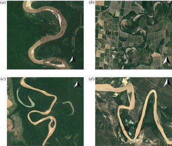
Examples of the occurrence of channel width oscillations associated with point bars (a,b and to a lesser extent in c) and mid-channel bars (c,d and to a lesser extent in a) in natural meandering rivers. (a) Rio Ucayali (Perù). (b) Sacramento River (USA). (c) Rio Beni (Bolivia). (d) Bermejo River (Paraguay). Images: 2015 DigitalGlobe, Landsat (landsat.usgs.gov).

The existence of both instream autogenic and allogenic triggering mechanisms for spatial width oscillations in meanders was already envisaged by Luchi et al. (Reference Luchi, Zolezzi and Tubino2010b ) and Zolezzi et al. (Reference Zolezzi, Luchi and Tubino2012b ). Observations suggest that where width variations are mainly caused by an autogenic mechanism, a mid-channel bar is found in the widest section, while a point bar dominates the widest section of a meandering river where the bank-driven mechanism is mainly responsible for spatial width oscillations. Figure 1 illustrates this concept by showing four examples of meandering river reaches with the widest sections located in correspondence of a point bar (a,b) and of a mid-channel bar (c,d). In figure 1(a,b) the two opposite banks seem to reveal different processes, due to the presence of a point bar at one bank (suggesting accretion) and a sharp transition from the wet channel to the vegetated floodplain at the other bank (suggesting erosion). Conversely, the presence of mid-channel bars in the widest sections of panels (c,d) suggests that both banks may undergo erosion, thus widening the river locally.
The above observations set the question of understanding how the autogenic and allogenic mechanisms interact during meander growth and how they might affect the planform evolution, leading to different evolutionary trajectories. Such understanding is constrained by the lack of a fully analytical modelling framework for the planform evolution of meandering rivers with oscillating width, because the models proposed so far rely on numerical solutions and therefore it is not easy to single out the role of different physical effects and fully explore the range of variability of flow parameters.
The first aim of this work is to develop a model, based on a fully analytical solution for the flow and bed topography, to investigate the temporal evolution of the planform of periodic sequences of meandering rivers, whose channel width is free to oscillate in time and space. The second aim is to apply the model to gain insight into the morphodynamic processes characterizing the mutual dynamics of channel width and curvature oscillations in evolving meandering rivers. The third aim is to check the model abilities and limitations to replicate observed behaviours, by comparing theoretical predictions with field data on real meandering rivers extracted from remotely sensed images.
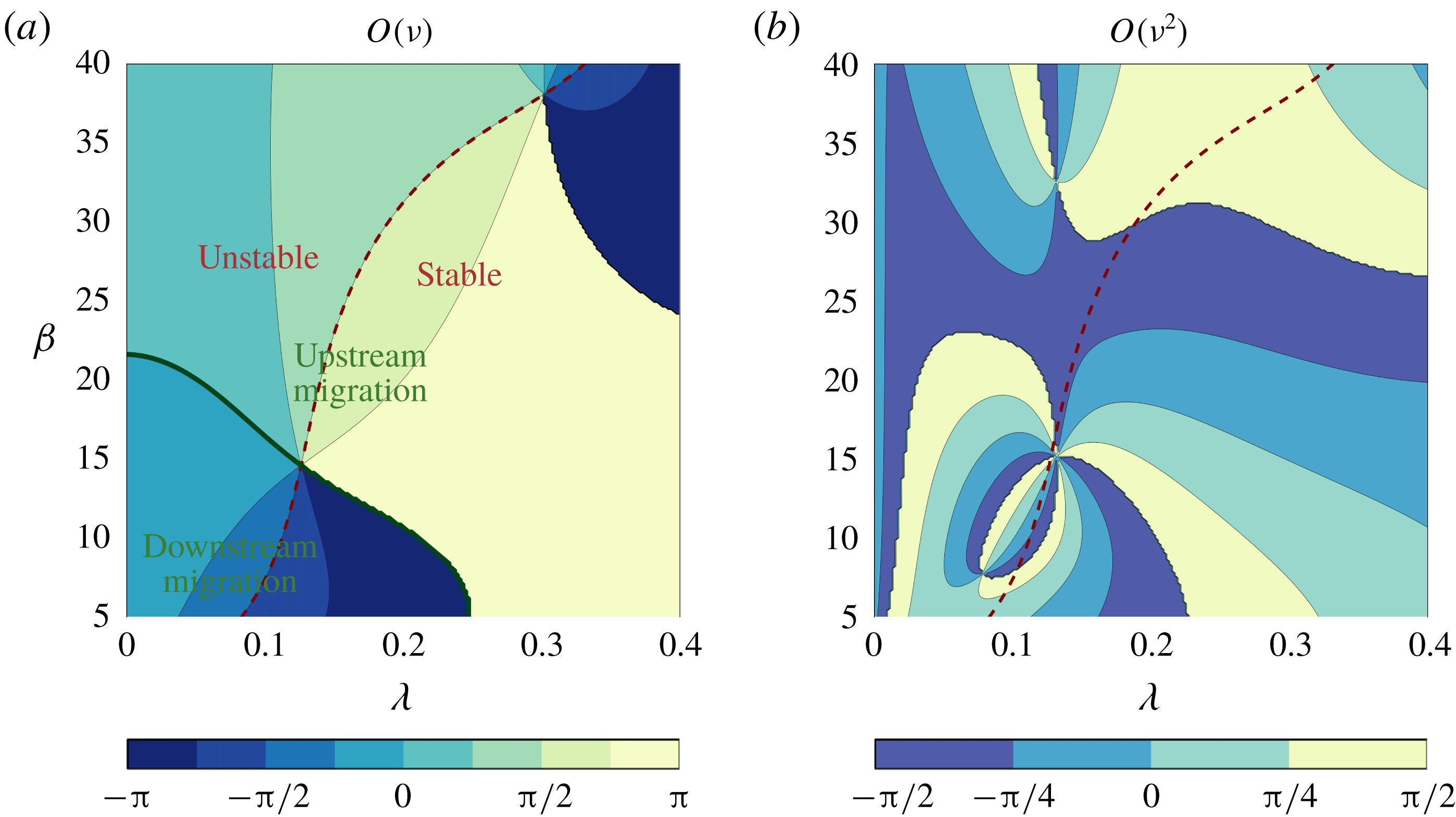
With these aims, we couple the integro-differential equation introduced by Seminara et al. (Reference Seminara, Zolezzi, Tubino and Zardi2001) to model the centreline evolution of equiwidth periodic meanders with a novel channel width evolution equation (§ 2.2). In the latter equation the migration law that relates the channel shift to the excess/defect of flow velocity at the banks is applied independently to each bank. Both equations are fed through the perturbation solution (§ 3) of the stand alone analytical description of the flow field and bed topography (the formulation is concisely recalled in § 2.1) previously obtained by different authors at the various orders of approximation, as summarized in table 1: the linear solution in equiwidth meanders (
 $O(\unicode[STIX]{x1D708})$
, e.g. Zolezzi & Seminara Reference Zolezzi and Seminara2001); the flow-bed topography linearly forced by spatial width oscillations in a straight channel (
 $O(\unicode[STIX]{x1D6FF})$
, e.g. Repetto et al.
Reference Repetto, Tubino and Paola2002); the nonlinear solution forced by curvature in an equiwidth channel (
 $O(\unicode[STIX]{x1D708}^{2})$
, e.g. Seminara & Tubino Reference Seminara and Tubino1992, Luchi et al.
Reference Luchi, Zolezzi and Tubino2010b
); the nonlinear effect of width oscillations on curvature (
 $O(\unicode[STIX]{x1D708}\unicode[STIX]{x1D6FF})$
, e.g. Luchi et al.
Reference Luchi, Zolezzi and Tubino2011).
On a methodological level, the primary scientific novelty of the present work is the implementation within an analytical framework of the coupled evolution of the channel axis and of the channel width in a periodic sequence of meanders, which was previously investigated only numerically. The fully analytical approach has the key advantage of allowing a clear isolation of different physical mechanisms controlling width evolution in space and time in evolving meanders, allowing us to clearly identify the forcing function of nonlinear curvature effects on autogenic width oscillations and the feedbacks of these oscillations on the centreline dynamics (§ 4). The presented field data have been extracted on purpose at local and at bend scales from remotely sensed images for model testing (§ 5). They quantify the temporal co-evolution of width and curvature for selected meander bends, information not previously available, which then represents an additional novelty of the work.
2 Model formulation
2.1 Flow field and sediment transport
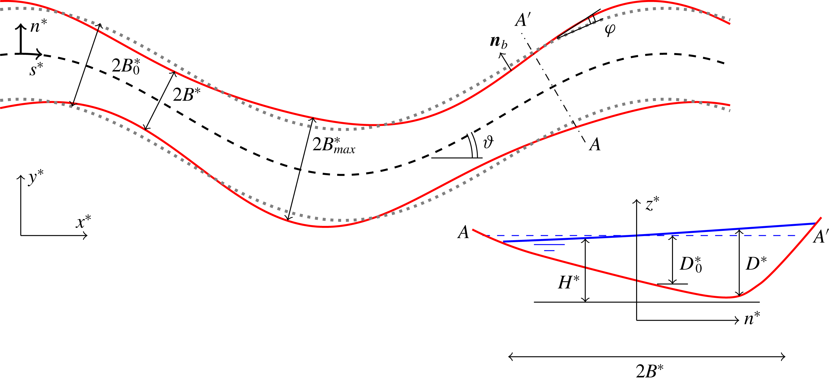
Sketch of a meandering reach with width variations and notation used in the mathematical model. In the cross-section the super-elevation of the free surface is represented (blue continuous line) with respect to the reference flow (blue dashed line). Notation as in Luchi et al. (Reference Luchi, Zolezzi and Tubino2011).

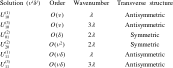
Perturbation solutions at different orders of approximation used in the present work. The perturbation parameters
 $(\unicode[STIX]{x1D708},\unicode[STIX]{x1D6FF})$
represent the dimensionless amplitudes of curvature and width oscillations, as defined in § 3.

We consider a periodic, sine-generated meandering river with variable width, a constant slope and uniform grain size
 $d_{s}^{\ast }$
. Figure 2 depicts the situation. Hydrodynamics and sediment transport are described by the two-dimensional depth-averaged model derived from the quasi-steady three-dimensional Reynolds-averaged Navier–Stokes equations coupled with the Exner equation. We adapt the above model to an intrinsic curvilinear coordinate reference system
 $(s^{\ast },n^{\ast })$
, where
 $s^{\ast }$
represents the longitudinal coordinate measured along the channel axis and
 $n^{\ast }$
is the transverse coordinate orthogonal to
 $s^{\ast }$
(hereafter an asterisk denotes dimensional quantities).
Let us define
 $$\begin{eqnarray}{\mathcal{C}}^{\ast }(s^{\ast })=-\frac{\unicode[STIX]{x2202}\unicode[STIX]{x1D717}}{\unicode[STIX]{x2202}s^{\ast }},\end{eqnarray}$$
the intrinsic curvature of the river reach measured along the channel axis, where
 $\unicode[STIX]{x1D717}$
is the inflection angle of channel centreline with respect to a Cartesian axis
 $x^{\ast }$
;
 $B^{\ast }(s^{\ast })$
the half-width of the channel, measured as orthogonal to the channel axis, and
 $\unicode[STIX]{x1D711}$
the local angle of the bank profile with respect to the channel axis, such that
 $$\begin{eqnarray}\tan \unicode[STIX]{x1D711}=\frac{\unicode[STIX]{x2202}B^{\ast }}{\unicode[STIX]{x2202}s^{\ast }}.\end{eqnarray}$$
We also conveniently define the following dimensionless quantities
 $$\begin{eqnarray}\displaystyle & \displaystyle (s,n)=({B_{0}^{\ast }}^{-1}s^{\ast },{B^{\ast }}^{-1}n^{\ast }), & \displaystyle\end{eqnarray}$$
 $$\begin{eqnarray}\displaystyle & \displaystyle (U,V)={U_{0}^{\ast }}^{-1}(U^{\ast },V^{\ast }), & \displaystyle\end{eqnarray}$$
 $$\begin{eqnarray}\displaystyle & \displaystyle (H,D)={D_{0}^{\ast }}^{-1}(F_{0}^{-2}H^{\ast },D^{\ast }), & \displaystyle\end{eqnarray}$$
 $$\begin{eqnarray}\displaystyle & \displaystyle (q_{s},q_{n})=(g^{\ast }\unicode[STIX]{x0394}{d_{s}^{\ast }}^{3})^{-(1/2)}(q_{s}^{\ast },q_{n}^{\ast }), & \displaystyle\end{eqnarray}$$
 $(U^{\ast },V^{\ast })$
are the components of the depth-averaged velocity vector,
 $H^{\ast }$
denotes the water surface elevation with respect to a reference horizontal plane,
 $D^{\ast }$
is the water depth,
 $\boldsymbol{q}^{\ast }=(q_{s}^{\ast },q_{n}^{\ast })$
is the bedload discharge vector per unit width. All these quantities are spatially variable, i.e. they depend on the spatial coordinates
 $(s,n)$
. Furthermore,
 $\unicode[STIX]{x1D6E5}$
is the relative submerged density, and
 $g^{\ast }$
is the gravity. The transverse coordinate
 $n$
has been stretched to match the local channel width, therefore lateral boundary conditions are to be imposed at
 $n=\pm 1$
. Furthermore,
 $U_{0}^{\ast },D_{0}^{\ast }$
and
 $F_{0}$
denote the mean velocity, depth and Froude number of the uniform flow that would occur, for the given discharge, grain size and slope, in an infinitely long rectangular channel of constant width
 $2B_{0}^{\ast }$
.
Such reference conditions can be unambiguously described by fixing the values of the following dimensionless parameters:
 $$\begin{eqnarray}\unicode[STIX]{x1D6FD}=\frac{B_{0}^{\ast }}{D_{0}^{\ast }},\quad \unicode[STIX]{x1D703}_{0}=\frac{{U_{0}^{\ast }}^{2}C_{0}}{g^{\ast }\unicode[STIX]{x0394}d_{s}^{\ast }},\quad d_{s}=\frac{d_{s}^{\ast }}{D_{0}^{\ast }},\end{eqnarray}$$
namely the aspect ratio, the Shields parameter and the relative roughness, where
 $C_{0}$
is the friction coefficient of the reference flow.
We then split the half-channel width in the form
 $$\begin{eqnarray}B^{\ast }(s^{\ast })=B_{0}^{\ast }+b^{\ast }(s^{\ast }),\end{eqnarray}$$
and conveniently define the longitudinal distributions of centreline curvature and half-width in the following dimensionless form:
 $$\begin{eqnarray}{\mathcal{C}}(s)={\mathcal{C}}^{\ast }R_{0}^{\ast },\quad B(s)=\frac{B^{\ast }}{B_{0}^{\ast }},\quad b(s)=\frac{2b^{\ast }}{B_{max}^{\ast }-B_{0}^{\ast }},\end{eqnarray}$$
where
 $R_{0}^{\ast }$
is a representative value of the channel radius of curvature (in the following twice the radius of curvature at the bend apex of a sine-generated channel centreline) and
 $B_{max}^{\ast }$
is the maximum value of the half-width within a meander wavelength. Substituting (2.5) and (2.6) into (2.1) and (2.2) we obtain
 $$\begin{eqnarray}\displaystyle & \displaystyle \frac{\unicode[STIX]{x2202}\unicode[STIX]{x1D717}}{\unicode[STIX]{x2202}s}=-\unicode[STIX]{x1D708}{\mathcal{C}}, & \displaystyle\end{eqnarray}$$
 $$\begin{eqnarray}\displaystyle & \displaystyle \tan \unicode[STIX]{x1D711}=\unicode[STIX]{x1D6FF}\frac{\unicode[STIX]{x2202}b}{\unicode[STIX]{x2202}s}, & \displaystyle\end{eqnarray}$$
 $\unicode[STIX]{x1D708}$
and the amplitude of the channel width oscillations
 $\unicode[STIX]{x1D6FF}$
,
 $$\begin{eqnarray}\unicode[STIX]{x1D708}=\frac{B_{0}^{\ast }}{R_{0}^{\ast }},\quad \unicode[STIX]{x1D6FF}=\frac{B_{max}^{\ast }-B_{0}^{\ast }}{2B_{0}^{\ast }}.\end{eqnarray}$$
Hereafter, the formulation for the flow field and sediment transport follows closely the one reported in Zolezzi et al. (Reference Zolezzi, Luchi and Tubino2012b ), which the interested reader is referred to. Here we briefly outline the main assumptions and closures adopted.
(i) Secondary flows are accounted for through a procedure originally introduced by Zolezzi & Seminara (Reference Zolezzi and Seminara2001), in which both dispersive terms and bed shear stresses associated with spiral flows due to streamline curvature are parameterized by coefficients
 $k_{i},i=0,\ldots ,5$
(see Zolezzi & Seminara Reference Zolezzi and Seminara2001, pp. 189–191). The total streamline curvature
${\mathcal{C}}_{s}(s,n)$
is computed as the sum of the curvature of the channel centreline and the curvature associated with local streamline deviation from channel centreline in the form (2.9)By employing streamline curvature we account for centrifugal effects (Luchi et al. Reference Luchi, Zolezzi and Tubino2011), while normal and tangential Reynolds stresses are neglected under the assumption of slowly varying flow field (Zolezzi & Seminara Reference Zolezzi and Seminara2001).$$\begin{eqnarray}{\mathcal{C}}_{s}=\unicode[STIX]{x1D708}{\mathcal{C}}-\frac{UV,_{s}-VU,_{s}}{U^{2}+V^{2}}.\end{eqnarray}$$
(ii) The local bed shear stress vector
$\unicode[STIX]{x1D749}(s,n)=(\unicode[STIX]{x1D70F}_{s}(s,n),\unicode[STIX]{x1D70F}_{n}(s,n))$
is defined as (2.10)where$$\begin{eqnarray}(\unicode[STIX]{x1D70F}_{s},\unicode[STIX]{x1D70F}_{n})=C\sqrt{U^{2}+V^{2}}(U,V+\unicode[STIX]{x1D70F}_{k}),\end{eqnarray}$$
(2.11)represents the secondary flow contribution and$$\begin{eqnarray}\unicode[STIX]{x1D70F}_{k}=\left[\frac{U{\mathcal{C}}_{s}D}{\unicode[STIX]{x1D6FD}\sqrt{C_{0}}}\left(k_{3}+\frac{k_{5}D,_{s}}{\unicode[STIX]{x1D6FD}\sqrt{C_{0}}}\right)+\frac{k_{4}D^{2}(U{\mathcal{C}}_{s}),_{s}}{\unicode[STIX]{x1D6FD}^{2}C_{0}}\right],\end{eqnarray}$$
$C$
is the local value of the friction coefficient. A commonly used logarithmic formula for rough open channel flow is employed to relate the spatially variable friction coefficient
$C(s,n)$
to the local water depth values (2.12)$$\begin{eqnarray}C(s,n)=\left[6+2.5\ln \left(\frac{D(s,n)}{2.5d_{s}}\right)\right]^{-2}.\end{eqnarray}$$
(iii) The components of the local sediment discharge
$[q_{s}(s,n),q_{n}(s,n)]$
, are expressed by means of the following relations which account for both shear stress and the downslope pull of gravity: where(2.13a )$$\begin{eqnarray}\displaystyle & \displaystyle q_{s}=\unicode[STIX]{x1D6F7}\left\{\cos \unicode[STIX]{x1D6FF}_{q}\left[1-\frac{1}{2}\left(\frac{\unicode[STIX]{x1D702},_{s}}{\unicode[STIX]{x1D6FD}(1+\unicode[STIX]{x1D708}\hat{n}{\mathcal{C}})}\right)^{2}\right]-\sin \unicode[STIX]{x1D6FF}_{q}\left(\frac{\unicode[STIX]{x1D702},_{s}\unicode[STIX]{x1D702},_{\hat{n}}}{\unicode[STIX]{x1D6FD}^{2}(1+\unicode[STIX]{x1D708}\hat{n}{\mathcal{C}})}\right)\right\},\qquad & \displaystyle\end{eqnarray}$$
(2.13b )$$\begin{eqnarray}\displaystyle & \displaystyle q_{n}=\unicode[STIX]{x1D6F7}\sin \unicode[STIX]{x1D6FF}_{q}\left[1-\frac{1}{2}\left(\frac{\unicode[STIX]{x1D702},_{n}}{\unicode[STIX]{x1D6FD}}\right)^{2}\right], & \displaystyle\end{eqnarray}$$
(2.14)$$\begin{eqnarray}\sin \unicode[STIX]{x1D6FF}_{q}(s,n)=\left(\frac{\unicode[STIX]{x1D70F}_{n}}{|\unicode[STIX]{x1D749}|}-\frac{r}{\unicode[STIX]{x1D6FD}\sqrt{\unicode[STIX]{x1D703}}}\unicode[STIX]{x1D702},_{\hat{n}}\right),\end{eqnarray}$$
$\unicode[STIX]{x1D6F7}=\unicode[STIX]{x1D6F7}(\unicode[STIX]{x1D703})$
is the bed load function,
$\unicode[STIX]{x1D702}=F_{0}^{2}H-D$
is the bed elevation,
$\hat{n}=nB$
,
$r$
is an empirical coefficient approximately equal to 0.5 (Talmon, Struiksma & Van Mierlo Reference Talmon, Struiksma and Van Mierlo1995),
$\unicode[STIX]{x1D703}(s,n)$
is the local value of the Shields parameter and
$\unicode[STIX]{x1D6FF}_{q}(s,n)$
denotes the local (spatially variable) angle formed by the local sediment transport rate vector with the streamwise coordinate
$s$
.The formula of Parker (Reference Parker1990) is employed to compute sediment transport, as representative of a class of transport formulae in which the exponent of the local Shields parameter in the dimensionless bedload function tends to the classical
$3/2$
value when
$\unicode[STIX]{x1D703}$
is far enough from the critical conditions for sediment mobility, the same exponent increasing for
$\unicode[STIX]{x1D703}$
approaching the critical value. Changing the bedload formula within the same class (e.g. Meyer-Peter & Müller Reference Meyer-Peter and Müller1948, Bagnold Reference Bagnold1966) has been shown not to qualitatively affect the outcomes of meander morphodynamic models (Zolezzi, Luchi & Tubino Reference Zolezzi, Luchi and Tubino2009). A local application of Parker’s formula, i.e. based on the local value of the Shields parameter
$\unicode[STIX]{x1D703}(s,n)$
has been chosen because it yields analogous results to the other ones and it is more suitable for an analytical implementation, thanks to the formal absence of a critical threshold.


The resulting two-dimensional model for the flow field and sediment transport reads
 $$\begin{eqnarray}\displaystyle & \displaystyle N{\mathcal{L}}_{b}(UD)+B^{-1}(VD),_{n}+N\unicode[STIX]{x1D708}{\mathcal{C}}VD=0, & \displaystyle\end{eqnarray}$$
 $$\begin{eqnarray}\displaystyle & \displaystyle NU{\mathcal{L}}_{b}(U)+B^{-1}VU,_{n}+N\unicode[STIX]{x1D708}{\mathcal{C}}UV+N{\mathcal{L}}_{b}(H)+N\unicode[STIX]{x1D6FD}\frac{\unicode[STIX]{x1D70F}_{s}}{D}=0, & \displaystyle\end{eqnarray}$$
 $$\begin{eqnarray}\displaystyle & \displaystyle NU{\mathcal{L}}_{b}(V)+B^{-1}VV,_{n}-N\unicode[STIX]{x1D708}{\mathcal{C}}U^{2}+B^{-1}H,_{n}+\unicode[STIX]{x1D6FD}\frac{\unicode[STIX]{x1D70F}_{n}}{D}=0, & \displaystyle\end{eqnarray}$$
 $$\begin{eqnarray}\displaystyle & \displaystyle N{\mathcal{L}}_{b}(q_{s})+B^{-1}(q_{n}),_{n}+N\unicode[STIX]{x1D708}{\mathcal{C}}q_{n}=0, & \displaystyle\end{eqnarray}$$
 $$\begin{eqnarray}N=\frac{1}{1+\unicode[STIX]{x1D708}nB{\mathcal{C}}},\quad {\mathcal{L}}_{b}=\frac{\unicode[STIX]{x2202}}{\unicode[STIX]{x2202}s}-\unicode[STIX]{x1D6FF}\frac{n}{B}\frac{\unicode[STIX]{x2202}b}{\unicode[STIX]{x2202}s}\frac{\unicode[STIX]{x2202}}{\unicode[STIX]{x2202}n},\end{eqnarray}$$
arise as a consequence of the metric coefficients of the adopted curvilinear system and of the stretching of the transverse variable needed to accommodate to width variations. In the system (2.15), a comma has been used to denote the partial derivative of an unknown with respect to an independent variable
 $(s,n)$
. System (2.15) has already been employed in several studies (see e.g. Zolezzi et al.
Reference Zolezzi, Luchi and Tubino2012b
) as the mathematical basis for deriving a spatially variable analytical solution for meandering rivers with variable channel width and curvature, and it contains all relevant physical effects relevant to such morphodynamic problem, which integrate inertial, redistribution and topographic effects due to the spatial variations of the forcing terms (
 ${\mathcal{C}}(s),b(s)$
) to the classical mechanisms controlling flow and bed topography in a constant curvature bend (transverse slope, centrifugal acceleration, superelevation of the free surface).
System (2.15) is associated with four boundary conditions in the lateral direction
 $n$
, imposing lateral impermeability to both flow and sediment discharge,
 $$\begin{eqnarray}(U,V)\boldsymbol{\cdot }\boldsymbol{n}_{b}=0,\quad (q_{s},q_{n})\boldsymbol{\cdot }\boldsymbol{n}_{b}=0,\quad (n=\pm 1),\end{eqnarray}$$
where
 $\boldsymbol{n}_{b}$
denotes the unit vector locally orthogonal to the banklines. In the longitudinal direction we impose periodic boundary conditions.
2.2 Planform evolution
To model the planform development of meandering rivers with spatially and temporally variable width, we integrate the planform evolution approach of Seminara et al. (Reference Seminara, Zolezzi, Tubino and Zardi2001) through an additional equation describing the temporal evolution of the spatial width oscillations.
The analysis is based on three key simplifying hypotheses. First, we assume the time scale of planform development to be sufficiently long to allow for the instantaneous adaptation of the flow field and bed topography to planform changes (curvature, width and length). This implies that as
 $\unicode[STIX]{x1D708}$
and
 $\unicode[STIX]{x1D6FF}$
coevolve in time, the flow and bed topography can be obtained from the steady solution of (2.15) and therefore they change in time only parametrically. Furthermore, on such a long time scale the bank migration process can be viewed as a continuous, rather than intermittent, process. Last, we focus our attention on width changes due to perturbations of flow field and bed topography with respect to the reference state. Therefore we assume that such a state, which changes slowly in time, does not produce any variation of the average channel width
 $2B_{0}^{\ast }$
.
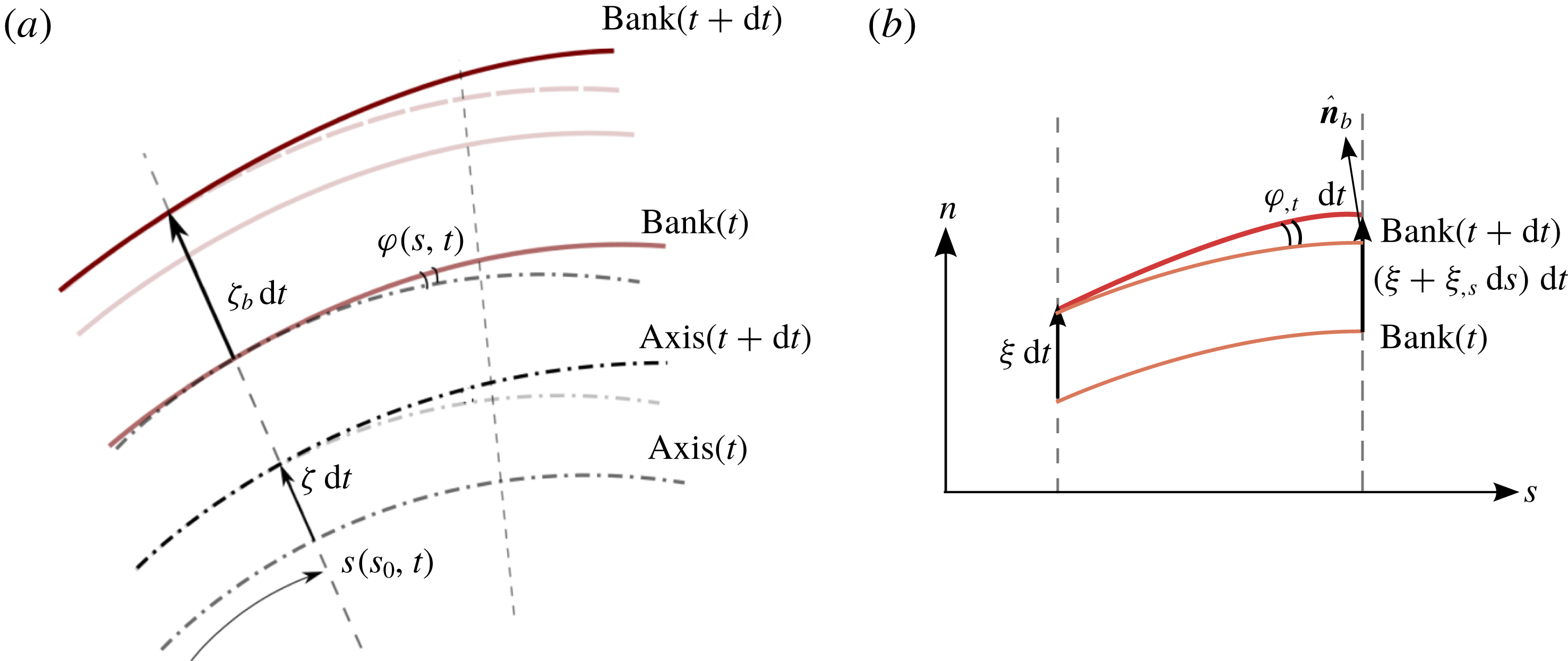
(a) Sketch of the model for planform development of channel axis and banks. (b) The model for bank development projected onto the curvilinear reference frame (the versor
 $\hat{\boldsymbol{n}}_{b}$
is locally orthogonal to the channel bank).

We refer to the geometrical construction reported in figure 3 to develop an evolutionary equation for the bank profile. Let us consider a local rate of migration of the channel bank
 $\unicode[STIX]{x1D701}_{b}$
, orthogonal to the channel axis, scaled with the reference velocity
 $U_{0}^{\ast }$
. The migration rate
 $\unicode[STIX]{x1D701}_{b}$
can be decomposed into a transversally antisymmetric contribution
 $\unicode[STIX]{x1D701}$
and a transversally symmetric contribution
 $\unicode[STIX]{x1D709}$
, such that
 $$\begin{eqnarray}\unicode[STIX]{x1D701}_{b}|_{n=\pm 1}=\unicode[STIX]{x1D701}\pm \unicode[STIX]{x1D709},\end{eqnarray}$$
where
 $n=\pm 1$
denote the outer and inner banks, respectively. Therefore,
 $\unicode[STIX]{x1D701}$
represents the lateral migration rate of the channel axis, while
 $\unicode[STIX]{x1D709}$
represents the local migration rate of the bank with respect to the channel axis. The additional equation for
 $\unicode[STIX]{x1D709}$
is obtained in the following form (see figure 3
b):
 $$\begin{eqnarray}\unicode[STIX]{x1D711},_{t}\cos (\unicode[STIX]{x1D711})^{-1}\,\text{d}t\,\text{d}s=\unicode[STIX]{x1D709},_{s}\,\text{d}s\cos (\unicode[STIX]{x1D711})\,\text{d}t,\end{eqnarray}$$
where
 $t$
is the dimensionless time, scaled with the flow time scale
 $B_{0}^{\ast }/U_{0}^{\ast }$
.
Hence, the planform evolution model for a meandering river with freely variable width is described by the following system of equations:
 $$\begin{eqnarray}\displaystyle & \displaystyle \unicode[STIX]{x1D717},_{t}-\unicode[STIX]{x1D717},_{s}\int _{0}^{s}\unicode[STIX]{x1D701}\unicode[STIX]{x1D717},_{s}\,\text{d}s=\unicode[STIX]{x1D701},_{s}, & \displaystyle\end{eqnarray}$$
 $$\begin{eqnarray}\displaystyle & \displaystyle \unicode[STIX]{x1D711},_{t}=\unicode[STIX]{x1D709},_{s}\cos ^{2}\unicode[STIX]{x1D711}. & \displaystyle\end{eqnarray}$$
Equation (2.20a
), which was first derived by Seminara et al. (Reference Seminara, Zolezzi, Tubino and Zardi2001), implies a cubic geometric nonlinearity in the evolution of the channel centreline. The integro-differential term in (2.20a
) accounts for the history of the deformation process of the channel centreline which affects the evolution of the channel axis. The cosine term in (2.20b
) is due to the different elongation of the bank with respect to the centreline and to the adopted definition of the bank migration rate
 $\unicode[STIX]{x1D709}$
as orthogonal to the channel axis. With
 $\unicode[STIX]{x1D701}$
the odd part of
 $\unicode[STIX]{x1D701}_{b}$
, we expect
 $\unicode[STIX]{x1D717}$
to be an odd function. This fact is enforced by the structure of (2.20a
), implying the cubic nonlinearity. On the other hand, we expect
 $\unicode[STIX]{x1D711}$
to be an even function, with
 $\unicode[STIX]{x1D709}$
being the even part of
 $\unicode[STIX]{x1D701}_{b}$
. The latter is enforced by the presence of the cosine term in the bank inflection equation (2.20b
).
When periodic, sine-generated meanders are of interest, the structure of equations (2.20) suggests a Fourier expansion of the variables
 $\unicode[STIX]{x1D717}$
and
 $\unicode[STIX]{x1D711}$
of the form
 $$\begin{eqnarray}\displaystyle & \displaystyle \unicode[STIX]{x1D717}(s,t)=\mathop{\sum }_{k=1}^{\infty }\unicode[STIX]{x1D717}_{m}(t)e_{m}+\text{c.c.},\quad e_{m}=\exp [\text{i}m\unicode[STIX]{x1D706}(t)s],\quad m=2k-1, & \displaystyle\end{eqnarray}$$
 $$\begin{eqnarray}\displaystyle & \displaystyle \unicode[STIX]{x1D711}(s,t)=\mathop{\sum }_{k=1}^{\infty }\unicode[STIX]{x1D711}_{m}(t)e_{m}+\text{c.c.},\quad m=2k, & \displaystyle\end{eqnarray}$$
 $\text{c.c.}$
represents the conjugate of a complex number and
 $\unicode[STIX]{x1D706}$
is the dimensionless meander wavenumber, scaled with the reference channel half-width
 $B_{0}^{\ast }$
. We note that
 $\unicode[STIX]{x1D706}$
is time dependent because meander sinuosity changes as curvature develops in time. We also note that only odd harmonics
 $(m=1,3,\ldots )$
need to be considered in (2.21a
) as a consequence of the cubic nonlinearity of (2.20a
).
Recalling (2.7b ), one can readily see that expansion (2.21b ) implies that the fundamental wavenumber of width oscillations is chosen as twice the wavenumber of curvature variations. This hypothesis relies on the assumption that each meander bend corresponds to an oscillation of channel width, which therefore displays two maxima over one meander wavelength. This is consistent with the few existing observations on real meanders (e.g. Seminara Reference Seminara2006, Luchi et al. Reference Luchi, Zolezzi and Tubino2011, Eke et al. Reference Eke, Czapiga, Viparelli, Shimizu, Imran, Sun and Parker2014a ) and is also implicit in Brice’s (Reference Brice1975) classification scheme for meandering rivers. Furthermore, the spatial structure set by (2.21b ) arises as a natural consequence of the autogenic nonlinear mechanism that produces width oscillations, as discussed in the next § 3.1.
If we keep only the first term of the expansion (2.21a ) we recover the classical sine-generated distribution. Using (2.7a ) we then obtain
 $$\begin{eqnarray}\unicode[STIX]{x1D708}=\unicode[STIX]{x1D706}|\unicode[STIX]{x1D717}_{1}|.\end{eqnarray}$$
Including also the second term of (2.21a ) we recover the Kinoshita (Reference Kinoshita1961) distribution of curvature, in dimensionless form
 $$\begin{eqnarray}{\mathcal{C}}=2[\cos (\unicode[STIX]{x1D706}s)-C_{F}\cos (3\unicode[STIX]{x1D706}s)-C_{S}\sin (3\unicode[STIX]{x1D706}s)],\end{eqnarray}$$
where
 $$\begin{eqnarray}C_{F}=-3\frac{\text{Im}(\unicode[STIX]{x1D717}_{3})}{|\unicode[STIX]{x1D717}_{1}|},\quad C_{S}=-3\frac{\text{Re}(\unicode[STIX]{x1D717}_{3})}{|\unicode[STIX]{x1D717}_{1}|},\end{eqnarray}$$
are the fattening and skewing coefficient, respectively.
Finally, a closure relation for the bank migration rate
 $\unicode[STIX]{x1D701}_{b}$
is required in order to solve (2.20). During the past years a number of models able to reproduce bank erosion and accretion mechanics leading to variations in channel width were developed. Mechanistic approaches for bank erosion processes were proposed by Duan & Julien (Reference Duan and Julien2005) and Chen & Duan (Reference Chen and Duan2006), who accounted for the sediment transport close to the banklines, and by Parker et al. (Reference Parker, Shimizu, Wilkerson, Eke, Abad, Lauer, Paola, Dietrich and Voller2011) and Motta, Abad & Garcia (Reference Motta, Abad and Garcia2012), who provided a physical description of the mechanics of bank processes such as the failure of slump blocks. Simplified models for bank erosion were proposed by Mosselman (Reference Mosselman1992), Darby et al. (Reference Darby, Alabyan and Van de Wiel2002), Jang & Shimizu (Reference Jang and Shimizu2005), Rüther & Olsen (Reference Rüther and Olsen2007), Darby, Rinaldi & Dapporto (Reference Darby, Rinaldi and Dapporto2007), while a rational, process-based description of bank accretion processes was provided by Zen et al. (Reference Zen, Zolezzi, Toffolon and Gurnell2016). However, including complex bank submodels into a perturbation scheme such as the one adopted in this paper is not straightforward. Simplified models able to approximately describe the key processes on longer time scales were widely used in the literature (Partheniades & Paaswell Reference Partheniades and Paaswell1970; Ikeda et al.
Reference Ikeda, Parker and Sawai1981; Seminara et al.
Reference Seminara, Zolezzi, Tubino and Zardi2001; Zolezzi et al.
Reference Zolezzi, Luchi and Tubino2012b
). They generally neglect bank boundary layers and the corresponding distribution of stresses at the bank and simply relate the lateral bank shift to the excess (defect) of flow velocity or stress at the bank toe. The latter assumption can be reasonable to estimate bank retreat even at the time scale of single flood events driving morphological change, while it strongly oversimplifies the complex depositional dynamics of bank advance that involves vegetation encroachment. However, besides the complexity of including a bank erosion/accretion model with a high level of detail into an analytical framework, we consider that on the long time scale of planform evolution of meandering rivers the differences in the processes that locally rule the advance and retreat of channel banks tend to be mitigated.
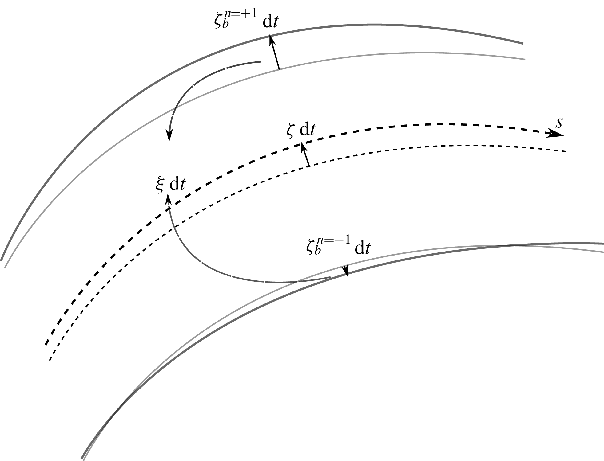
In Seminara et al. (Reference Seminara, Zolezzi, Tubino and Zardi2001) the centreline’s migration rate is assumed to be proportional to the difference between the velocity at the outer bank and that at the inner bank. A novel element in our approach, which is needed to allow width to locally evolve, is the possibility for each bank to migrate independently. The concept underpinning such novel formulation is graphically illustrated in figure 4. Namely, the migration rate of each bank is set as proportional to the difference between the velocity at the bank and a threshold value, here assumed to coincide with the reference flow velocity
 $U_{0}^{\ast }$
. In dimensionless form, such a bank migration model reads
 $$\begin{eqnarray}\unicode[STIX]{x1D701}_{b}^{n=\pm 1}=\pm 2E(U|_{n=\pm 1}-1),\end{eqnarray}$$
where
 $E$
is a lateral migration coefficient, which typically takes values in the range
 $10^{-7}{-}10^{-8}$
(Camporeale et al.
Reference Camporeale, Perona, Porporato and Ridolfi2005), and the factor 2 has been added for consistency with the traditional method. It must be noted that the time scale of simulated meander planform development in a real case study crucially depends on the choice of the lateral migration coefficient
 $E$
, which has been shown to actually represent a calibration parameter (Crosato Reference Crosato2009) for model testing against multi-temporal observations on channel centreline evolution.
We also note that the ratio between the planform time scale
 $T_{E}\sim B_{0}^{\ast }/EU_{0}^{\ast }$
and the bed time scale
 $T_{B}\sim B_{0}^{\ast }D_{0}^{\ast }/\sqrt{g^{\ast }\unicode[STIX]{x0394}{D_{s}^{\ast }}^{3}}\unicode[STIX]{x1D6F7}(\unicode[STIX]{x1D703}_{0})$
takes the order of magnitude of
 $10^{1}{-}10^{3}$
in natural meandering rivers, which justifies the assumption of instantaneous adaptation of flow and bed topography to planform changes.
Sketch of decoupled bank migration model and notation.

Equations (2.25) are then combined is such a way that half their difference and their average give rise to the centreline migration rate
 $\unicode[STIX]{x1D701}$
and to the local width change rate
 $\unicode[STIX]{x1D709}$
, respectively,
 $$\begin{eqnarray}\displaystyle & \displaystyle \unicode[STIX]{x1D701}={\textstyle \frac{1}{2}}(\unicode[STIX]{x1D701}_{b}^{n=+1}+\unicode[STIX]{x1D701}_{b}^{n=-1})=E(U|_{n=+1}-U|_{n=-1}), & \displaystyle\end{eqnarray}$$
 $$\begin{eqnarray}\displaystyle & \displaystyle \unicode[STIX]{x1D709}={\textstyle \frac{1}{2}}(\unicode[STIX]{x1D701}_{b}^{n=+1}-\unicode[STIX]{x1D701}_{b}^{n=-1}-2)=E(U|_{n=+1}+U|_{n=-1}-2). & \displaystyle\end{eqnarray}$$
 $U_{0}^{\ast }$
implies that we neglect the adaptation of the average channel width to the slow time change of the reference flow due to meander elongation. Although the latter process could be easily incorporated into the model (see for instance Eke et al. (Reference Eke, Czapiga, Viparelli, Shimizu, Imran, Sun and Parker2014a
)), we adopt here such approximation in order to single out the role of flow and bed perturbations.
3 Mathematical solution
3.1 Perturbation approach
The two-dimensional hydrodynamics and sediment transport problem (2.15) is solved analytically by means of a second-order two parameter (
 $\unicode[STIX]{x1D708}$
,
 $\unicode[STIX]{x1D6FF}$
) expansion. The analysis is based on the recognition that the values of
 $\unicode[STIX]{x1D708}$
and
 $\unicode[STIX]{x1D6FF}$
are typically much smaller than unity in real meandering rivers. For instance, Zolezzi et al. (Reference Zolezzi, Luchi and Tubino2012b
) examined the spatial series of curvature and width for the class-C bends reported in the large dataset of Lagasse et al. (Reference Lagasse, Zevenbergen, Spitz, Thorne, Associates and Collins2004) showing that average
 $\unicode[STIX]{x1D6FF}$
values are typically slightly less than
 $0.1$
, with values up to
 $\unicode[STIX]{x1D6FF}\simeq 0.2$
for very few bends, while
 $\unicode[STIX]{x1D708}$
falls in the range 0.05–0.2 and rarely exceeds
 $0.25$
.
Hence, we employ the following expansion of the unknown variables:
 $$\begin{eqnarray}\displaystyle \boldsymbol{V} & = & \displaystyle \boldsymbol{V}_{0}+\unicode[STIX]{x1D708}(\boldsymbol{V}_{10}^{(1)}C_{1}e_{1}+\boldsymbol{V}_{10}^{(3)}C_{3}e_{3}+\text{c.c.})+\unicode[STIX]{x1D6FF}(\boldsymbol{V}_{01}^{(2)}b_{2}e_{2}+\text{c.c.})\nonumber\\ \displaystyle & & \displaystyle +\,\unicode[STIX]{x1D708}^{2}(\boldsymbol{V}_{20}^{(2)}C_{1}^{2}e_{2}+\text{c.c.})+\unicode[STIX]{x1D708}\unicode[STIX]{x1D6FF}(\boldsymbol{V}_{11}^{(1)}\bar{C}_{1}b_{2}e_{1}+\boldsymbol{V}_{11}^{(3)}C_{1}b_{2}e_{3}+\text{c.c.}),\end{eqnarray}$$
where
 $\boldsymbol{V}_{ij}^{(k)}=(U_{ij}^{(k)},\boldsymbol{V}_{ij}^{(k)},H_{ij}^{(k)},D_{ij}^{(k)})^{\text{T}}$
,
 $\boldsymbol{V}_{0}=(1,0,H_{0}(s),1)^{\text{T}}$
and the overbar (
 $\,\bar{\;}\,$
) denotes the conjugate of a complex number. Note that analogous perturbation expansions are performed for the Shields parameter, friction coefficient, bed shear stresses, sediment fluxes, which are therefore variable along the meandering channel as they are functions of (
 $s,n$
) through their nonlinear dependences on the local values of the four fundamental unknowns (
 $U$
,
 $V$
,
 $H$
,
 $D$
), as expressed by the closure relations (2.9)–(2.13) and on the local curvature values, as expressed by (3.1). In order to keep the analysis as simple as possible, yet retaining the fundamental interactions between curvature and width variations, we have included the first two terms of the curvature distribution arising from (2.21a
) and the fundamental component of width oscillations
 $$\begin{eqnarray}{\mathcal{C}}(s)=C_{1}e_{1}+C_{3}e_{3}+\text{c.c.},\quad b(s)=b_{2}e_{2}+\text{c.c.}\end{eqnarray}$$
Furthermore, in (3.1) we have only considered the nonlinear terms (
 $\unicode[STIX]{x1D708}\unicode[STIX]{x1D6FF}$
,
 $\unicode[STIX]{x1D708}^{2}$
) that arise from the interaction between the fundamental components (
 $e_{1}$
,
 $e_{2}$
) of curvature and width distributions and we have neglected the
 $O(\unicode[STIX]{x1D708}^{2},\unicode[STIX]{x1D6FF}^{2})$
nonlinear distortion of the basic reference flow.
Finally, let us briefly explain why the second-order contribution
 $O(\unicode[STIX]{x1D6FF}^{2})$
has not been incorporated. In a dominant-mode periodic analysis, we only consider the first harmonic of each longitudinal signal. The
 $O(\unicode[STIX]{x1D708})$
contribution has a
 $\unicode[STIX]{x1D706}$
periodicity, while the
 $O(\unicode[STIX]{x1D6FF})$
contribution has a
 $2\unicode[STIX]{x1D706}$
periodicity;
 $N$
th-order terms have
 $N\unicode[STIX]{x1D706}$
periodicity, i.e.
 $O(\unicode[STIX]{x1D708}^{2})$
has
 $2\unicode[STIX]{x1D706}$
periodicity (hence it interacts with the width oscillation), while
 $O(\unicode[STIX]{x1D708}\unicode[STIX]{x1D6FF})$
has both a
 $\unicode[STIX]{x1D706}$
and a
 $3\unicode[STIX]{x1D706}$
periodicity;
 $O(\unicode[STIX]{x1D6FF}^{2})$
has a
 $4\unicode[STIX]{x1D706}$
periodicity, hence it does not affect the fundamental and can be left out from the analysis.
The solution (3.1) is used to feed the planform evolution model (2.20) through the bank and centreline migration relations (2.26).
The
 $O(\unicode[STIX]{x1D708})$
linear solution represents the classical flow field solution forced by the presence of linearly forced bars in a regular sequence of sine-generated meander bends; its analytical solution has been employed for a long time in the analysis of meander stability (Blondeaux & Seminara Reference Blondeaux and Seminara1985) and evolution (Seminara et al.
Reference Seminara, Zolezzi, Tubino and Zardi2001). Its transversal structure is antisymmetric and oscillates longitudinally with the same frequency as the curvature.
The
 $O(\unicode[STIX]{x1D6FF})$
linear solution was first derived by Repetto et al. (Reference Repetto, Tubino and Paola2002) and represents the flow-bed topography response to a periodically varying width along a straight reach. Its transverse structure is symmetrical, giving rise to a spatial sequence of mid-channel bars.
The
 $O(\unicode[STIX]{x1D708}^{2})$
nonlinear self-interaction has a transversal symmetric structure and it may be the cause of the presence of mid-channel bars in meandering rivers, as shown by Luchi et al. (Reference Luchi, Hooke, Zolezzi and Bertoldi2010a
). Being transversally symmetrical, it is the leading curvature perturbation that can interact with width variation in the processes of local widening and narrowing because of the same transverse structure. Moreover, its wavenumber intrinsically emerges as twice that of the curvature, consistently with the assumption made on channel width in (2.21b
).
The
 $O(\unicode[STIX]{x1D708}\unicode[STIX]{x1D6FF})$
nonlinear mixed interaction is instead antisymmetrical and embodies the effect of width variations on bend dynamics (Luchi et al.
Reference Luchi, Zolezzi and Tubino2011), because its spatial structure exactly corresponds to that of the
 $O(\unicode[STIX]{x1D708})$
first-order solution. Expansion (3.1) suggests that width oscillations also affect the development of the third longitudinal harmonic
 $e_{3}$
of curvature distribution, which is responsible for fattening and skewing of meander shape, through the term
 $\boldsymbol{V}_{11}^{(3)}$
. The role of such contribution, which was not previously investigated, may turn out to be relevant in the final stage of meander evolution as the role of
 $e_{3}$
component becomes significant at relatively high sinuosity.
Symmetry properties and wavenumbers of the perturbation solutions for the longitudinal velocity
 $U_{ij}$
.

Symmetry properties of the perturbation solution at different orders are summarized in table 2. We note that, from the mathematical point of view, the channel width of meandering rivers is continuously forced towards spatial oscillations (
 $O(\unicode[STIX]{x1D708}^{2})$
effect). In summary, mutual feedbacks between width and curvature are primarily accounted for in the
 $O(\unicode[STIX]{x1D708}^{2})$
solution and in
 $O(\unicode[STIX]{x1D708}\unicode[STIX]{x1D6FF})$
solution (Luchi et al.
Reference Luchi, Zolezzi and Tubino2011). More details on the relation between the solution at different perturbation orders can be found in Zolezzi et al. (Reference Zolezzi, Luchi and Tubino2012b
).
3.2 Perturbation solution
Substituting the expansion (3.1) into the system (2.15) we derive an ordinary differential system in the transverse direction for each unknown at every order of the perturbation expansion, which can be conveniently written in matrix form for any system of order
 $O(\unicode[STIX]{x1D708}^{i}\unicode[STIX]{x1D6FF}^{j})$
,
 $$\begin{eqnarray}\left(\begin{array}{@{}cccc@{}}a_{11}^{ij} & a_{12}^{ij}\displaystyle \frac{\text{d}}{\text{d}n} & a_{13}^{ij} & a_{14}^{ij}\\ a_{21}^{ij} & a_{22}^{ij} & a_{23}^{ij}\displaystyle \frac{\text{d}}{\text{d}n} & a_{24}^{ij}\\ a_{31}^{ij} & a_{32}^{ij}\displaystyle \frac{\text{d}}{\text{d}n} & a_{33}^{ij} & a_{34}^{ij}\\ a_{41}^{ij} & a_{42}^{ij}\displaystyle \frac{\text{d}}{\text{d}n} & a_{43}^{ij}\displaystyle \frac{\text{d}^{2}}{\text{d}n^{2}} & a_{44}^{ij}+a_{45}^{ij}\displaystyle \frac{\text{d}^{2}}{\text{d}n^{2}}\end{array}\right)\left(\begin{array}{@{}c@{}}U_{ij}\\ V_{ij}\\ H_{ij}\\ D_{ij}\end{array}\right)=\left(\begin{array}{@{}c@{}}b_{1}^{ij}(n)\\ b_{2}^{ij}(n)\\ b_{3}^{ij}(n)\\ b_{4}^{ij}(n)\end{array}\right),\end{eqnarray}$$
where the coefficients
 $a_{lk}^{ij}$
are analogous to those computed by Luchi et al. (Reference Luchi, Zolezzi and Tubino2011), while the coefficients
 $b_{l}^{ij}$
are the forcing terms arising from nonlinear interaction between lower-order terms. Each system of equations can be easily solved analytically once lateral boundary conditions are imposed (2.17); they take the form
 $$\begin{eqnarray}\left(V_{ij},\frac{\text{d}(F_{0}^{2}H-D)}{\text{d}n}\right)=\pm (b_{ij}^{5},b_{ij}^{6}),\quad (n=\pm 1).\end{eqnarray}$$
The solution of (3.3) yields the transverse structure of the perturbations of flow field and bed topography at the different orders of approximation. Here we focus on the longitudinal velocity perturbations, which in the present approach (2.25) are responsible for bank migration. In particular, solutions
 $U_{10}$
and
 $U_{11}$
are antisymmetric and therefore involved in bend amplification, while
 $U_{20}$
and
 $U_{01}$
, both being symmetric, regulate autogenic width adjustments along meander bends.
Substituting the perturbation solutions into (2.26) we obtain the components of the lateral migration rate
 $\unicode[STIX]{x1D701}$
of the channel centreline and of the local rate
 $\unicode[STIX]{x1D709}$
of width change in the form,
 $$\begin{eqnarray}\displaystyle & \displaystyle \unicode[STIX]{x1D701}_{1}=(\unicode[STIX]{x1D708}C_{1}U_{10}^{(1)}+\unicode[STIX]{x1D708}\unicode[STIX]{x1D6FF}\bar{C}_{1}b_{2}U_{11}^{(1)})_{n=1}, & \displaystyle\end{eqnarray}$$
 $$\begin{eqnarray}\displaystyle & \displaystyle \unicode[STIX]{x1D701}_{3}=(\unicode[STIX]{x1D708}C_{3}U_{10}^{(3)}+\unicode[STIX]{x1D708}\unicode[STIX]{x1D6FF}C_{1}b_{2}U_{11}^{(3)})_{n=1}, & \displaystyle\end{eqnarray}$$
 $$\begin{eqnarray}\displaystyle & \displaystyle \unicode[STIX]{x1D709}_{2}=(\unicode[STIX]{x1D6FF}b_{2}U_{01}^{(2)}+\unicode[STIX]{x1D708}^{2}C_{1}^{2}U_{20}^{(2)})_{n=1}, & \displaystyle\end{eqnarray}$$
 $$\begin{eqnarray}\unicode[STIX]{x1D701}=2E(\unicode[STIX]{x1D701}_{1}e_{1}+\unicode[STIX]{x1D701}_{3}e_{3}+\text{c.c.}),\quad \unicode[STIX]{x1D709}=2E(\unicode[STIX]{x1D709}_{2}e_{2}+\text{c.c.}).\end{eqnarray}$$
It is important to note that the antisymmetric perturbations of the flow field act on the centreline migration rate
 $\unicode[STIX]{x1D701}$
, while symmetrical perturbations either force or damp the local widening rate
 $\unicode[STIX]{x1D709}$
. Therefore, from a linear point of view, the curvature forced
 $\unicode[STIX]{x1D708}$
-perturbation produces effects on meander amplification, while the
 $\unicode[STIX]{x1D6FF}$
-perturbation, forced by width variation, affects the width changes. From the two-dimensional analysis of Repetto et al. (Reference Repetto, Tubino and Paola2002), the
 $O(\unicode[STIX]{x1D6FF})$
linear solution for the longitudinal velocity at the bank (the first term on the right-hand side of (3.5c
)) turns out to invariably produce a self-suppressing effect, at least for the values of the wavenumber relevant for the present analysis. Therefore, the only mechanism able to produce width variation is the autogenic effect related to the second-order solution for curvature perturbation,
 $O(\unicode[STIX]{x1D708}^{2})$
.
Expansions (2.21) and (3.6) are finally incorporated into the planimetric evolution model (2.20). The resulting system of ordinary differential equations eventually reads
 $$\begin{eqnarray}\displaystyle & \displaystyle \frac{\text{d}\unicode[STIX]{x1D717}_{1}}{\text{d}T}=\text{i}\unicode[STIX]{x1D706}\left[(A+\bar{A})\unicode[STIX]{x1D717}_{1}-\frac{A_{2}}{2}\bar{\unicode[STIX]{x1D717}}_{1}+\frac{3}{2}\bar{A}_{2}\unicode[STIX]{x1D717}_{3}-\frac{3}{4}A_{4}\bar{\unicode[STIX]{x1D717}}_{3}+\unicode[STIX]{x1D701}_{1}\right], & \displaystyle\end{eqnarray}$$
 $$\begin{eqnarray}\displaystyle & \displaystyle \frac{\text{d}\unicode[STIX]{x1D717}_{3}}{\text{d}T}=\text{i}\unicode[STIX]{x1D706}\left[3(A+\bar{A})\unicode[STIX]{x1D717}_{3}+\frac{A_{2}}{2}\unicode[STIX]{x1D717}_{1}-\frac{\bar{A}_{4}}{4}\unicode[STIX]{x1D717}_{1}-\frac{A_{6}}{2}\bar{\unicode[STIX]{x1D717}}_{3}+3\unicode[STIX]{x1D701}_{3}\right], & \displaystyle\end{eqnarray}$$
 $$\begin{eqnarray}\displaystyle & \displaystyle \frac{\text{d}\unicode[STIX]{x1D706}}{\text{d}T}=\text{i}\unicode[STIX]{x1D706}^{2}(A_{0}-\bar{A}_{0}), & \displaystyle\end{eqnarray}$$
 $$\begin{eqnarray}\displaystyle & \displaystyle \frac{\text{d}\unicode[STIX]{x1D711}_{2}}{\text{d}T}=2\text{i}\unicode[STIX]{x1D706}[\unicode[STIX]{x1D709}_{2}(1-2|\unicode[STIX]{x1D711}_{2}|^{2})-\unicode[STIX]{x1D711}_{2}^{2}\bar{\unicode[STIX]{x1D709}}_{2}], & \displaystyle\end{eqnarray}$$
 $E$
has been absorbed into the dimensionless time,
 $T=2Et$
, consistently with (2.25), and
 $$\begin{eqnarray}\displaystyle & \displaystyle A_{0}=\bar{\unicode[STIX]{x1D701}_{1}}\unicode[STIX]{x1D717}_{1}+3\bar{\unicode[STIX]{x1D701}_{3}}\unicode[STIX]{x1D717}_{3}, & \displaystyle\end{eqnarray}$$
 $$\begin{eqnarray}\displaystyle & \displaystyle A_{2}=\unicode[STIX]{x1D701}_{1}\unicode[STIX]{x1D717}_{1}+3\bar{\unicode[STIX]{x1D701}_{1}}\unicode[STIX]{x1D717}_{3}-\unicode[STIX]{x1D701}_{3}\bar{\unicode[STIX]{x1D717}_{1}}, & \displaystyle\end{eqnarray}$$
 $$\begin{eqnarray}\displaystyle & \displaystyle A_{4}=\unicode[STIX]{x1D701}_{3}\unicode[STIX]{x1D717}_{1}+3\unicode[STIX]{x1D701}_{1}\unicode[STIX]{x1D717}_{3}, & \displaystyle\end{eqnarray}$$
 $$\begin{eqnarray}\displaystyle & \displaystyle A_{6}=3\unicode[STIX]{x1D701}_{3}\unicode[STIX]{x1D717}_{3}, & \displaystyle\end{eqnarray}$$
 $$\begin{eqnarray}\displaystyle & \displaystyle A=-\left(\frac{A_{2}}{2}+\frac{A_{4}}{4}+\frac{A_{6}}{6}\right). & \displaystyle\end{eqnarray}$$
Equations (3.7a,b
) describe the temporal evolution of the centreline curvature, while (3.7c
) quantifies meander elongation as curvature and width coevolve. These equations are formally identical to those derived by Seminara et al. (Reference Seminara, Zolezzi, Tubino and Zardi2001) for constant width meanders. However, the terms on the right-hand side include the effect of width oscillations which is felt through the dependence on
 $\unicode[STIX]{x1D6FF}$
of the components of the migration rate
 $\unicode[STIX]{x1D701}_{1},\unicode[STIX]{x1D701}_{3}$
(3.5a,b
). Therefore, their solution is coupled with that of (3.7d
) describing the temporal evolution of width oscillations, which in turn is affected by curvature through the dependence of
 $\unicode[STIX]{x1D709}_{2}$
on the autogenic
 $O(\unicode[STIX]{x1D708}^{2})$
term appearing in (3.5c
). As a limiting case, system (3.7) can be reduced to the classical constant width case by setting
 $\unicode[STIX]{x1D6FF}=0$
. On the other hand, the evolutionary solution for a straight channel with periodic width oscillations can be obtained by setting
 $\unicode[STIX]{x1D708}=0$
.
The solution of (3.7) has been computed by means of a variable-coefficient ordinary differential equation system solver with fixed-leading-coefficient implementation, backward differentiation method and adaptive numerical time step (Brown, Byrne & Hindmarsh Reference Brown, Byrne and Hindmarsh1989) in order to achieve both stability and a good level of accuracy (Jones et al.
Reference Jones, Oliphant and Peterson2001). The initial condition has been set in terms of a small amplitude sine-generated meander, whose initial wavenumber is
 $\unicode[STIX]{x1D706}_{0}$
, with given initial values of the reference flow parameters (
 $\unicode[STIX]{x1D6FD}$
,
 $\unicode[STIX]{x1D703}_{0}$
and
 $d_{s}$
), while
 $\unicode[STIX]{x1D711}$
has been set equal to zero. At each time step the complex coefficients that describe the distribution of curvature and width oscillations in (3.2) are computed through (2.7) in the following form
 $$\begin{eqnarray}\unicode[STIX]{x1D708}C_{m}=-m\text{i}\unicode[STIX]{x1D706}\unicode[STIX]{x1D717}_{m}\quad (m=1,3),\quad \unicode[STIX]{x1D6FF}b_{2}=-\frac{\text{i}\unicode[STIX]{x1D711}_{2}}{2\unicode[STIX]{x1D706}}.\end{eqnarray}$$
Recalling the definitions (2.8) and (2.22) of the parameters
 $\unicode[STIX]{x1D708}$
and
 $\unicode[STIX]{x1D6FF}$
, one can readily prove that
 $|C_{1}|=|b_{2}|=1$
.
4 Results
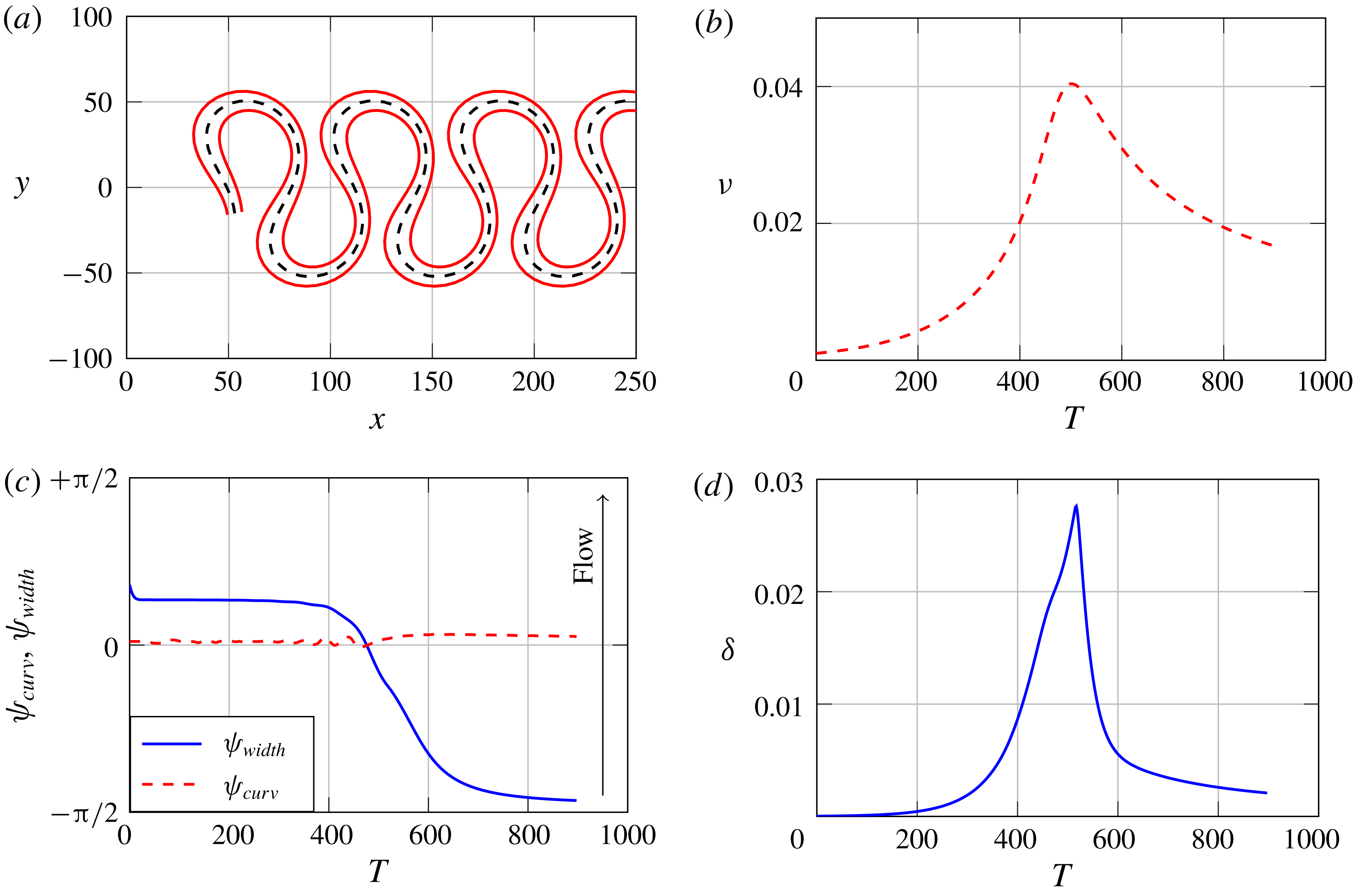
Evolutionary dynamics of a sub-resonant meander with autogenic width oscillations. (a) Planform shape with centreline and banklines at
 $T=790$
. (b) Temporal evolution of the curvature ratio
 $\unicode[STIX]{x1D708}$
. (c) Phase lag of the bend apex,
 $\unicode[STIX]{x1D713}_{curv}$
, and of the widest section,
 $\unicode[STIX]{x1D713}_{width}$
, with respect to the half-bend longitudinal position. Lag values of
 $-\unicode[STIX]{x03C0}/2$
(
 $+\unicode[STIX]{x03C0}/2$
) correspond to the upstream (downstream) meander inflection. (d) Temporal evolution of the dimensionless amplitude of width variations
 $\unicode[STIX]{x1D6FF}$
. Initial values of parameters:
 $\unicode[STIX]{x1D6FD}=10$
,
 $d_{s}=0.01$
,
 $\unicode[STIX]{x1D703}_{0}=0.1$
,
 $\unicode[STIX]{x1D706}_{0}=0.1$
,
 $|\unicode[STIX]{x1D717}_{1}|=0.01$
.

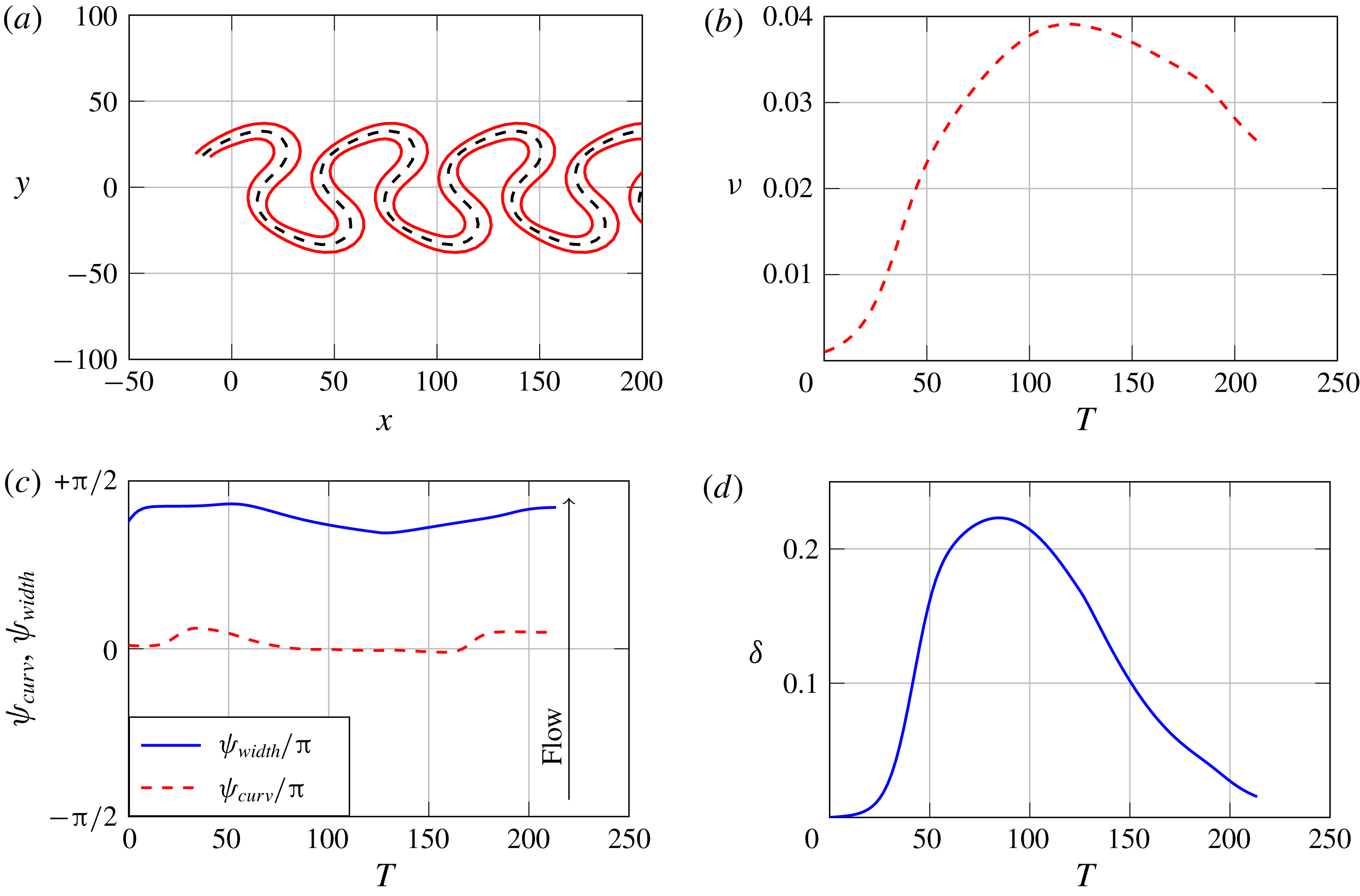
Evolutionary dynamics of a super-resonant meander with autogenic width oscillations. (a) Planform shape with centreline and banklines at
 $T=193$
. (b) Temporal evolution of the curvature ratio
 $\unicode[STIX]{x1D708}$
. (c) Phase lag of the bend apex,
 $\unicode[STIX]{x1D713}_{curv}$
, and of the widest section,
 $\unicode[STIX]{x1D713}_{width}$
, with respect to the half-bend longitudinal position. Lag values of
 $-\unicode[STIX]{x03C0}/2$
(
 $+\unicode[STIX]{x03C0}/2$
) correspond to the upstream (downstream) meander inflection. (d) Temporal evolution of the dimensionless amplitude of width variations
 $\unicode[STIX]{x1D6FF}$
. Initial values of parameters:
 $\unicode[STIX]{x1D6FD}=20$
,
 $d_{s}=0.01$
,
 $\unicode[STIX]{x1D703}_{0}=0.1$
,
 $\unicode[STIX]{x1D706}_{0}=0.1$
,
 $|\unicode[STIX]{x1D717}_{1}|=0.01$
.

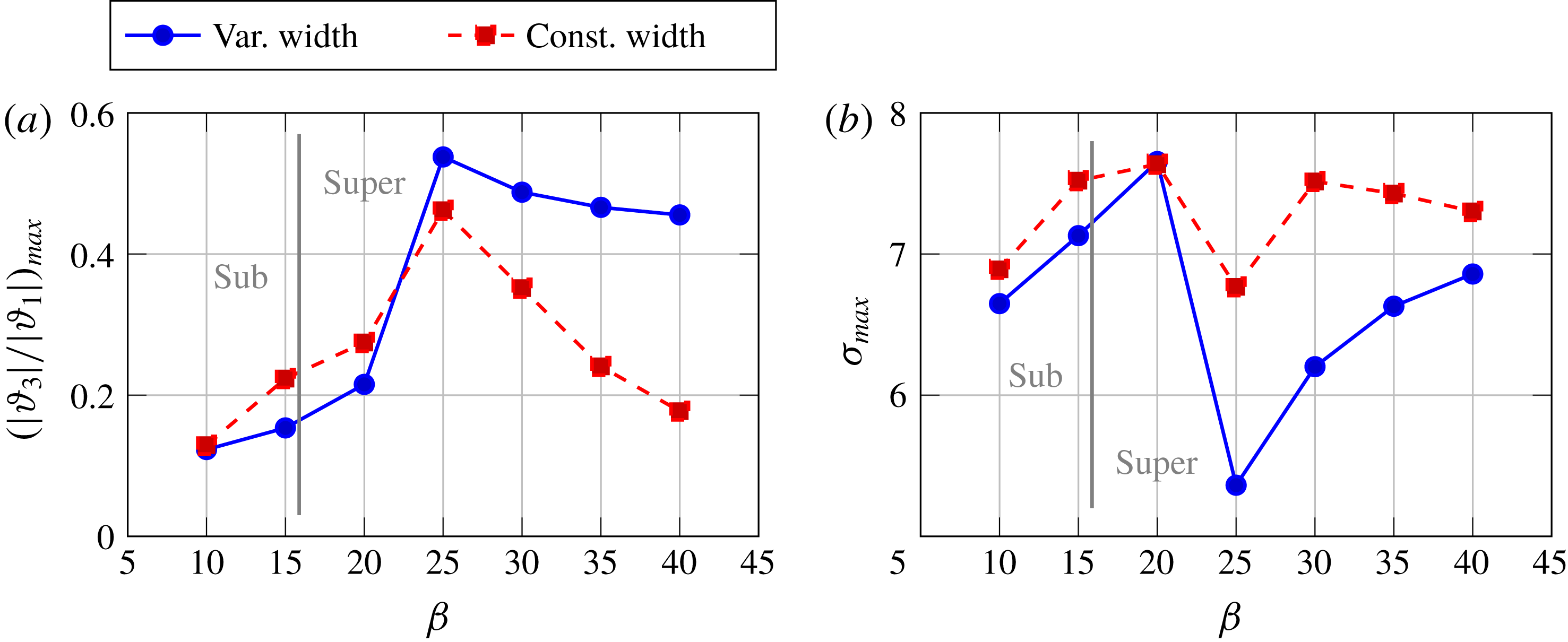
Effect of the autogenic width variations on the meander shape parameters: comparison between variable width (solid lines) and constant width simulations (dashed lines) as a function of the width ratio
 $\unicode[STIX]{x1D6FD}$
. (a) The ratio between the maximum amplitude of the third and the first harmonic of the centreline inflection angle
 $\unicode[STIX]{x1D717}$
. (b) Channel sinuosity evaluated at cutoff. Initial values of parameters:
 $d_{s}=0.01$
,
 $\unicode[STIX]{x1D703}_{0}=0.1$
,
 $\unicode[STIX]{x1D706}_{0}=0.1$
.

We first investigate the coevolution of curvature and width oscillations as the meander develops in time.
In the absence of width variations the evolutionary dynamics of channel curvature consists of an initial stage characterized by the growth of the fundamental harmonic (
 $e_{1}$
), while channel sinuosity keeps relatively small, followed by a second stage in which meander length, and therefore sinuosity, increases quite rapidly and higher-order components develop through nonlinear effects (see Seminara et al.
Reference Seminara, Zolezzi, Tubino and Zardi2001, figures 5–7). Such a two-stage process is reflected in the temporal evolution of the curvature ratio
 $\unicode[STIX]{x1D708}$
, which initially grows to a maximum value and then declines in a second stage due to the increase of the intrinsic meander length.
The model of Seminara et al. (Reference Seminara, Zolezzi, Tubino and Zardi2001) also suggests that the planform shape strongly depends on the width ratio
 $\unicode[STIX]{x1D6FD}$
falling below or above the resonant value
 $\unicode[STIX]{x1D6FD}_{R}$
. Sub-resonant meanders are typically downstream skewed, while super-resonant meanders exhibit upstream skewed loops and are prone to evolving much faster, as cutoff occurs at lower values of the rescaled time
 $T$
. It is useful to remember that the term ‘resonant’ refers to the unbounded response of the linear
 $O(\unicode[STIX]{x1D708})$
solution which occurs, for given values of
 $\unicode[STIX]{x1D703}_{0}$
and
 $d_{s}$
, as
 $\unicode[STIX]{x1D6FD}$
exactly matches
 $\unicode[STIX]{x1D6FD}_{R}$
(Blondeaux & Seminara Reference Blondeaux and Seminara1985). The dependence of the resonant aspect ratio
 $\unicode[STIX]{x1D6FD}_{R}$
on Shields parameter and grain roughness can be found in Seminara & Tubino (Reference Seminara and Tubino1992) (figure 4).
The above distinction between sub- and super-resonant meanders turns out to be relevant also in the present case in which width variations are taken into account, as their role on planform development is markedly different in the two regimes.
Figures 5 and 6 show the evolution of sub- and super-resonant meanders. The initial parameter values are the same in the two cases, but for the width ratio
 $\unicode[STIX]{x1D6FD}$
, which falls below (figure 5) or above (figure 6) the resonant value (
 $\unicode[STIX]{x1D6FD}_{R}\simeq 15.8$
). Figures 5(a) and 6(a) show the meander planform, at
 $T=790$
and
 $T=193$
, respectively, which reflects the assumption of channel width oscillating at a double spatial frequency compared to centreline curvature and displays downstream (
 $\unicode[STIX]{x1D6FD}<\unicode[STIX]{x1D6FD}_{R}$
) and upstream (
 $\unicode[STIX]{x1D6FD}>\unicode[STIX]{x1D6FD}_{R}$
) skewed loops. The evolution in time of the curvature ratio
 $\unicode[STIX]{x1D708}$
and of the dimensionless amplitude of width oscillations
 $\unicode[STIX]{x1D6FF}$
is reported in figures 5(b) and 6(b) and in figures 5(d) and 6(d), respectively. The behaviour of the parameter
 $\unicode[STIX]{x1D708}$
is rather similar to that observed in constant width channels and is governed (see 2.22) by the opposing effects of the growth of
 $\unicode[STIX]{x1D717}_{1}$
, which characterizes the first phase, and the decrease of meander wavenumber that dominates the second phase, when channel sinuosity mainly develops.
The effect of width variations on the curvature ratio
 $\unicode[STIX]{x1D708}$
is negligible in sub-resonant regime, as shown in figure 5(b), while it becomes relevant for
 $\unicode[STIX]{x1D6FD}>\unicode[STIX]{x1D6FD}_{R}$
, leading to a time delay of the peak curvature and slowing down the decline of curvature in the final stage of planform development (figure 6
b). On the other hand, the behaviour of the amplitude of width oscillations is closely related to that of curvature, as its growth is driven by the
 $O(\unicode[STIX]{x1D708}^{2})$
autogenic term appearing in (3.5c
), which results in a sharp increase of
 $\unicode[STIX]{x1D6FF}$
until a peak is reached (figures 5
c and 6
c). Such an effect is counterbalanced by the linear
 $O(\unicode[STIX]{x1D6FF})$
term of (3.5c
) that always produces a suppressing contribution, which increases with
 $\unicode[STIX]{x1D6FF}$
. The amplitude of width oscillations keeps relatively small in the sub-resonant case, while it becomes large for a longer time in the super-resonant case, being more persistently close to the peak value of nearly
 $0.2$
.
Figures 5(c) and 6(c) show the locations of the bend apex and of the widest section with respect to the inflection points. They are expressed in terms of the phase lags,
 $\unicode[STIX]{x1D713}_{curv}$
and
 $\unicode[STIX]{x1D713}_{width}$
, respectively, measured with reference to the half-bend section (therefore
 $-\unicode[STIX]{x03C0}/2$
and
 $\unicode[STIX]{x03C0}/2$
denote the positions of two consecutive inflection points). In both sub- and super-resonant cases the bend apex keeps nearly in phase with the half-bend section during meander evolution and deviates from this location only slightly due to nonlinear effects. On the other hand, the behaviour of
 $\unicode[STIX]{x1D713}_{width}$
is markedly different in the two cases. In the sub-resonant case (figure 5
d) the phase lag
 $\unicode[STIX]{x1D713}_{width}$
undergoes a strong variation in time, such that the widest section is initially located downstream of the bend apex, and progressively slides back to the upstream inflection. On the contrary, in the super-resonant case (figure 6
d) the position of the widest section is fairly stable in time and keeps closer to the inflection point.
A summary of the effect of autogenic width variations on the centreline evolution is given in figure 7, where the maximum amplitude of the third harmonic
 $\unicode[STIX]{x1D717}_{3}$
of the inflection angle, scaled with that of the fundamental
 $\unicode[STIX]{x1D717}_{1}$
(figure 7
a), and channel sinuosity (
 $\unicode[STIX]{x1D70E}=\unicode[STIX]{x1D706}_{0}/\unicode[STIX]{x1D706}$
; figure 7
b), evaluated at cutoff are reported for different values of the width ratio
 $\unicode[STIX]{x1D6FD}$
. Results of the present theory are compared with those of equiwidth simulations, for the same set of parameters. At low values of
 $\unicode[STIX]{x1D6FD}$
width variations tend to suppress the geometrical nonlinearities and produce more regular meander shapes with limited relevance of the third harmonic. However, as
 $\unicode[STIX]{x1D6FD}$
crosses the resonant range such an effect is reversed and becomes stronger, thus promoting the fattening and skewing of the meander shape in the final stage of evolution. Furthermore, when width variations are taken into account, the elongation of super-resonant meanders is strongly inhibited and therefore channel sinuosity attains smaller values, as shown in figure 7(b), falling to a minimum for values of
 $\unicode[STIX]{x1D6FD}$
above the resonant range.
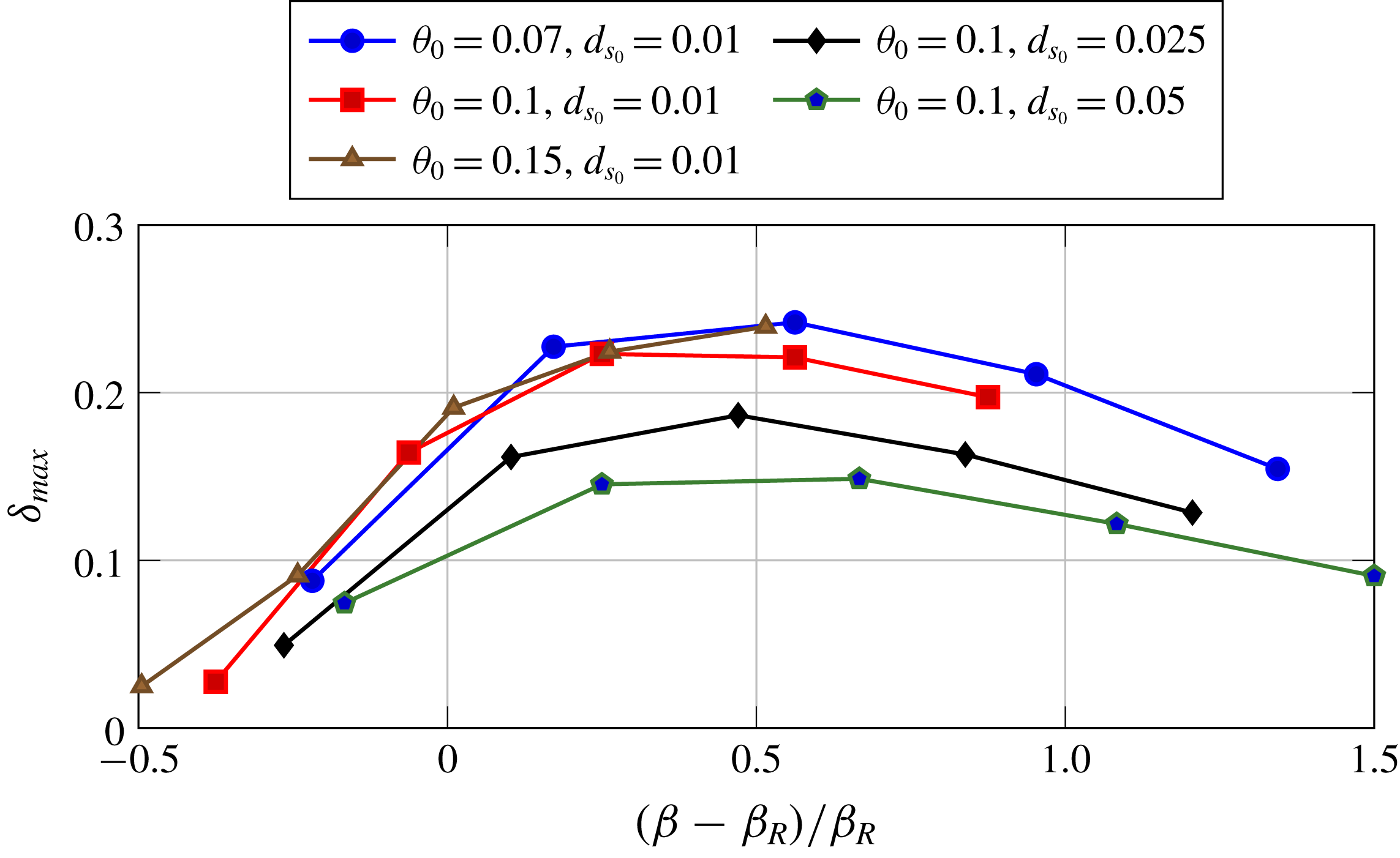
The peak amplitude
 $\unicode[STIX]{x1D6FF}_{max}$
of width variations as a function of the aspect ratio, measured with respect to its resonant value
 $\unicode[STIX]{x1D6FD}_{R}$
, for different sets of initial flow conditions (
 $\unicode[STIX]{x1D703}_{0}$
,
 $d_{s}$
) and initial meander wavenumber
 $\unicode[STIX]{x1D706}_{0}=0.1$
.

The position of the widest section
 $\unicode[STIX]{x1D713}_{width}$
along half a meander wavelength between two consecutive apexes as a function of the width ratio, measured with respect to its resonant value
 $\unicode[STIX]{x1D6FD}_{R}$
, for different sets of initial flow conditions (
 $\unicode[STIX]{x1D703}_{0}$
,
 $d_{s}$
) and initial meander wavenumber
 $\unicode[STIX]{x1D706}_{0}=0.1$
. The values of
 $\unicode[STIX]{x1D713}_{width}$
are computed when the width oscillation amplitude reaches its peak.

The maximum floodplain width
 $\unicode[STIX]{x0394}y_{max}$
, scaled with the reference channel width, as a function of the width ratio, measured with respect to its resonant value
 $\unicode[STIX]{x1D6FD}_{R}$
, for different sets of initial flow conditions (
 $\unicode[STIX]{x1D703}$
,
 $d_{s}$
) and initial meander wavenumber
 $\unicode[STIX]{x1D706}_{0}=0.1$
(full markers). Empty markers refer to the results of the equiwidth model (
 $\unicode[STIX]{x1D6FF}=0$
).

Such behaviour highlights the suppressing attitude of autogenic width variations on the activity of super-resonant meanders. A clear explanation can be given in the dependence of
 $\unicode[STIX]{x1D6FF}$
on flow parameters. Computing the peak value
 $\unicode[STIX]{x1D6FF}_{max}$
for different values of the reference parameters (
 $\unicode[STIX]{x1D6FD}$
,
 $\unicode[STIX]{x1D703}_{0}$
and
 $d_{s}$
) and measuring the width ratio
 $\unicode[STIX]{x1D6FD}$
with respect to
 $\unicode[STIX]{x1D6FD}_{R}$
, which depends on
 $\unicode[STIX]{x1D703}_{0}$
and
 $d_{s}$
, a fairly coherent scenario is obtained, as shown in figure 8. The value of
 $\unicode[STIX]{x1D6FF}_{max}$
exhibits a sharp increase as we move from sub-resonant to super-resonant meanders, reaches a maximum for
 $\unicode[STIX]{x1D6FD}$
nearly equal to
 $1.5\unicode[STIX]{x1D6FD}_{R}$
and then declines for larger
 $\unicode[STIX]{x1D6FD}$
(here and in the following figures the initial values of
 $\unicode[STIX]{x1D6FD}$
are 10, 15, 20, 25, 30). Figure 8 also shows that the amplitude of width oscillations is almost unaffected by
 $\unicode[STIX]{x1D703}_{0}$
, while it drops as the sediment gets coarser.
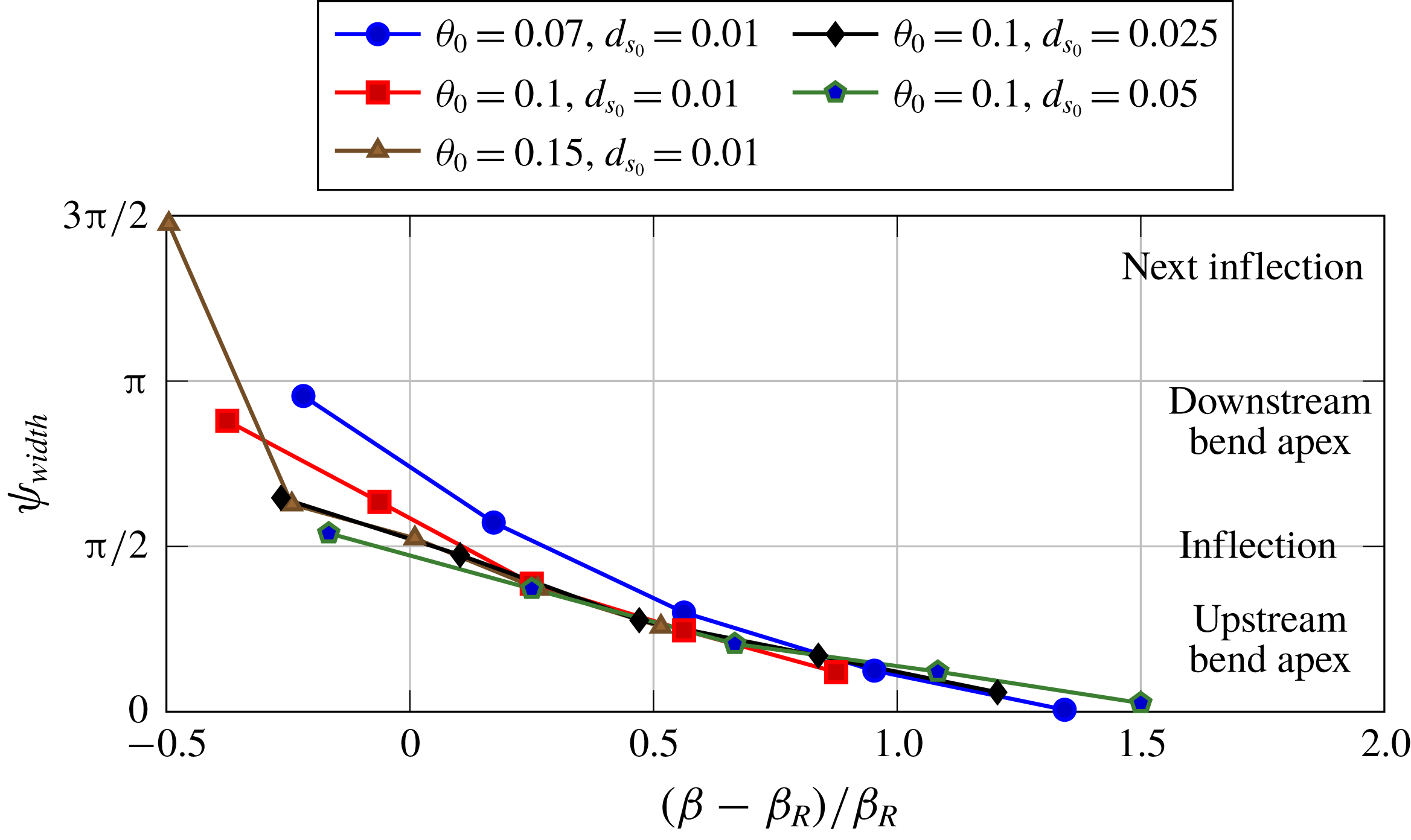
The position of the widest section when
 $\unicode[STIX]{x1D6FF}$
reaches its peak also exhibits a similar coherent behaviour, as the different curves overlap, at least in the super-resonant regime, once they are represented in terms of the relative distance from the resonant state. Figure 9 suggests that the widest section is approximately located at the meander inflection at resonance; furthermore, it slides back from downstream to upstream of the inflection point as
 $\unicode[STIX]{x1D6FD}$
crosses the resonant value, and eventually reaches the upstream bend apex for wide channels. Comparing figures 8 and 9 it can be noted that the widest section is located half-way between the apex and the inflection point (
 $\unicode[STIX]{x1D713}_{width}\simeq \unicode[STIX]{x03C0}/4$
) in the range of
 $\unicode[STIX]{x1D6FD}$
values corresponding to the maximum amplification of width oscillations (
 $\unicode[STIX]{x1D6FD}\simeq 1.5\unicode[STIX]{x1D6FD}_{R}$
). We note that the effect of the initial meander wavenumber
 $\unicode[STIX]{x1D706}_{0}$
on width oscillations is straightforward, with
 $\unicode[STIX]{x1D6FF}$
quadratically forced by the curvature
 $\unicode[STIX]{x1D708}$
, that in turn linearly depends on
 $\unicode[STIX]{x1D706}$
(see (2.22)). Hence, in the unstable wavenumber range,
 $\unicode[STIX]{x1D6FF}_{max}$
increases for increasing values of
 $\unicode[STIX]{x1D706}_{0}$
.
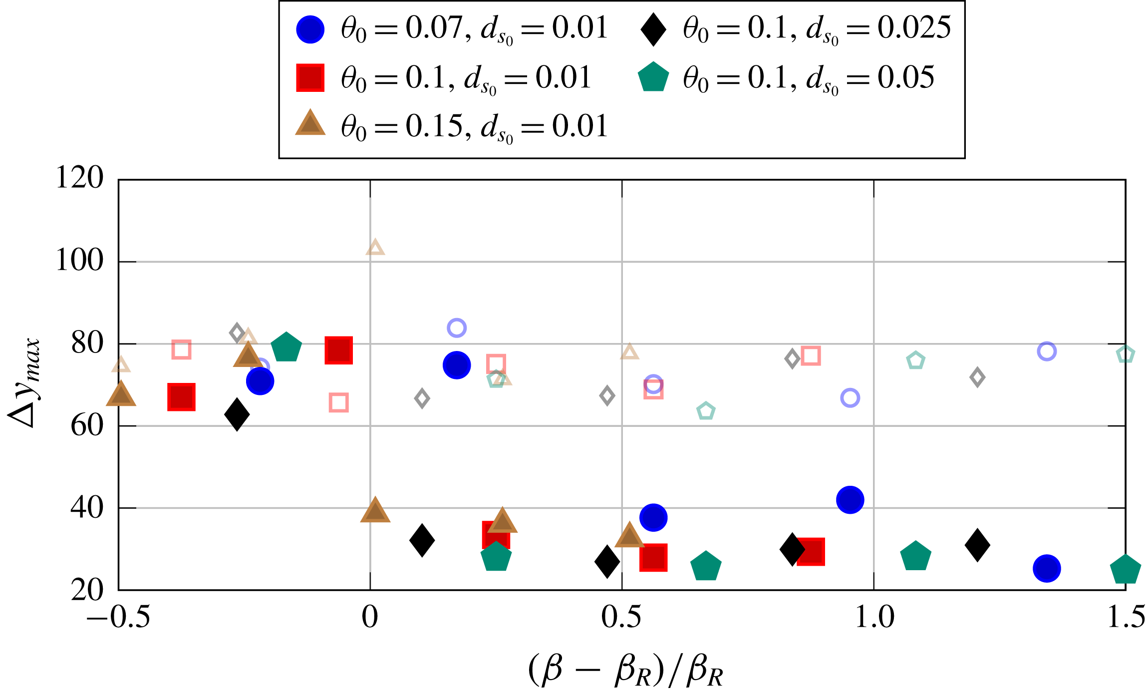
Further evidence of the different evolutionary dynamics of sub- and super-resonant meanders can be obtained through the analysis of the width of the floodplain which is needed to accommodate meander development from the initial stage until cutoff. In figure 10 we report (with full markers) the envelope of the river belt width, measured as the maximum transverse distance between two consecutive bend apexes, for the same set of parameters of figures 8 and 9. Results of our model highlight the existence of a sharp transition as the width ratio crosses the resonant value: sub-resonant meanders seem to require more space to develop, nearly 60–80 times their width, while super-resonant meanders keep more confined and the belt width drops to 20–40 times the channel width. As shown in figure 10 results of equiwidth simulations (empty markers) do not display a similar dependence on
 $\unicode[STIX]{x1D6FD}$
. Therefore, such distinct behaviour seems inherently associated with the effect of autogenic width variations on meander development.
Temporal hysteresis curves in the coevolution of curvature and width variations in developing meanders, for different values of the aspect ratio
 $\unicode[STIX]{x1D6FD}$
. Initial conditions:
 $d_{s}=0.01,\unicode[STIX]{x1D703}_{0}=0.1,\unicode[STIX]{x1D706}_{0}=0.1$
.

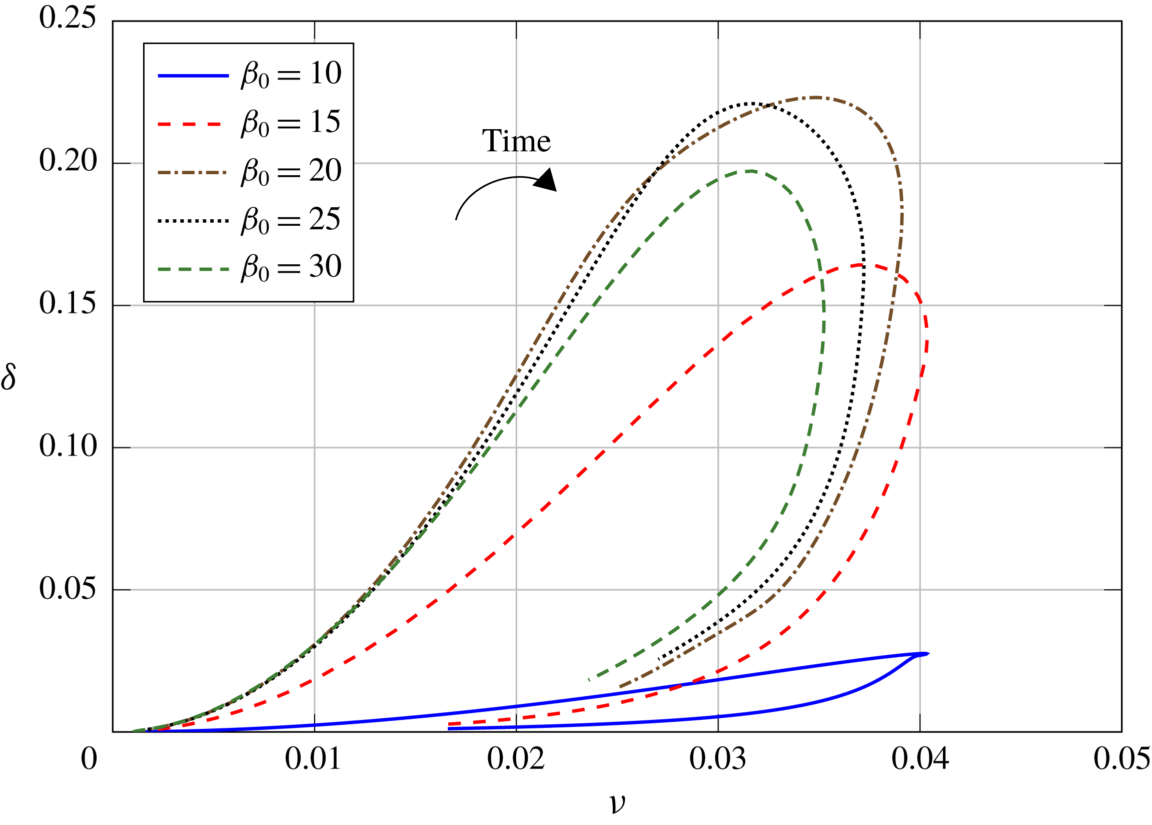
Coevolution and mutual interaction between autogenic width oscillations and curvature, as they emerge from the present model, can be further visualized through curves representing meander planform evolution in the (
 $\unicode[STIX]{x1D708},\unicode[STIX]{x1D6FF}$
) parameter space (figure 11). In the first stage of meander development width oscillation amplitude is forced quadratically by curvature through the
 $O(\unicode[STIX]{x1D708}^{2})$
term. Furthermore, the peak of width variations often occurs earlier than the peak of curvature, leading to a temporal hysteresis whose amplitude is mainly controlled by the width ratio
 $\unicode[STIX]{x1D6FD}$
. Hysteresis curves show that the peak of curvature ratio
 $\unicode[STIX]{x1D708}$
depends on the characteristics of the flow field only slightly, weakly decreasing with the aspect ratio, while the peak of
 $\unicode[STIX]{x1D6FF}$
changes with
 $\unicode[STIX]{x1D6FD}$
as illustrated in figure 8.
5 Field observations and theoretical predictions
A comparison of model predictions with field data would require the availability of a comprehensive data set on width variations dynamics in developing meanders, which is presently lacking (Dubón Reference Dubón2018). While a systematic comparison is therefore beyond the scope of the present work, we explore to which extent the predictions of our theoretical model are realistic and able to reproduce observed evolutionary tendencies in variable width meanders. We use a combination of the few information available in existing datasets with an explorative novel analysis of remotely sensed data that we performed to detect the evolutionary behaviour of variable width, naturally evolving meandering rivers.
In the following we highlight how model predictions reproduce at least qualitatively, observed features. Namely, we focus on the following aspects: the dimensionless width variation amplitude
 $\unicode[STIX]{x1D6FF}$
, the overall sinuosity (compared to the equiwidth case), the temporal hysteresis of bend evolution in the (
 $\unicode[STIX]{x1D708}$
,
 $\unicode[STIX]{x1D6FF}$
) space and the time evolution of the parameters
 $\unicode[STIX]{x1D708}$
and
 $\unicode[STIX]{x1D6FF}$
throughout the process of meander development.
Available field observations confirm the predicted tendency of variable width meanders to behave differently from their equiwidth counterparts and their specific tendency to display lower sinuosity values (Luchi et al.
Reference Luchi, Zolezzi and Tubino2011). Moreover, various investigations carried out at the reach scale (e.g. Knighton Reference Knighton1972, Richards Reference Richards1976, Hooke Reference Hooke1986, Luchi et al.
Reference Luchi, Zolezzi and Tubino2010b
) provide field evidence that autogenic processes can be important to drive spatial variations of channel width associated with the formation of central bars (the nonlinear
 $O(\unicode[STIX]{x1D708}^{2})$
contribution in the present theory).
Our analytical model suggests that width oscillations mainly develop under super-resonant conditions and attain peak values, expressed in terms of the dimensionless amplitude
 $\unicode[STIX]{x1D6FF}$
, falling in the range
 $0.15\div 0.22$
, for the sets of flow conditions examined. The above range of predicted
 $\unicode[STIX]{x1D6FF}$
-values is consistent with the results of field observations. Zolezzi et al. (Reference Zolezzi, Luchi and Tubino2012b
) analysed the large database compiled by Lagasse et al. (Reference Lagasse, Zevenbergen, Spitz, Thorne, Associates and Collins2004), where different styles of meandering were identified depending upon the intensity of spatial width oscillations, and found that width variation amplitudes of meandering rivers are generally of the order of
 $O(10^{-1})$
and rarely attain values as large as
 $0.2$
.
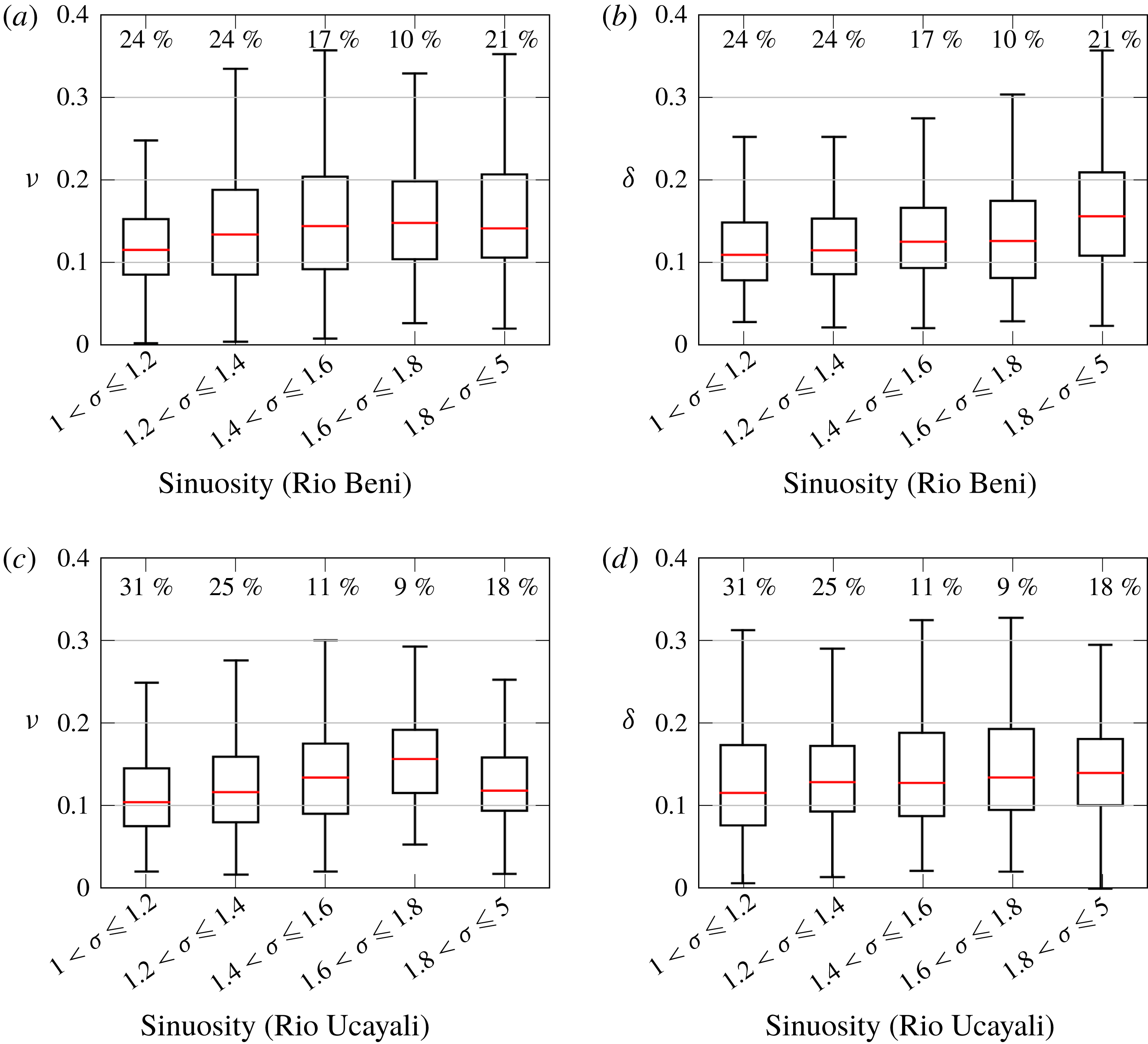
We integrate such field information with some novel field data that we extracted through a preliminary analysis of the evolutionary dynamics of width and curvature of some meander bends of two large dynamic subtropical rivers, the Rio Beni (Bolivian Amazon) and the Rio Ucayali (Peruvian Amazon). The analysis was conducted through the software PyRIS for multi-temporal meander morphodynamic analyses from remotely sensed images (Monegaglia et al. Reference Monegaglia, Zolezzi, Güneralp, Henshaw and Tubino2018). Each individual bend was isolated for each Landsat image frame (roughly one per year for thirty consecutive years between 1985 and 2015), and a bend-scale analysis was performed to determine the local values of planform parameters (width, curvature, Cartesian and intrinsic length). The examined reaches (400 km for the Rio Beni and 900 km for the Rio Ucayali) included nearly 240 and 270 meander bends respectively. Some of the bends could be monitored until cutoff.
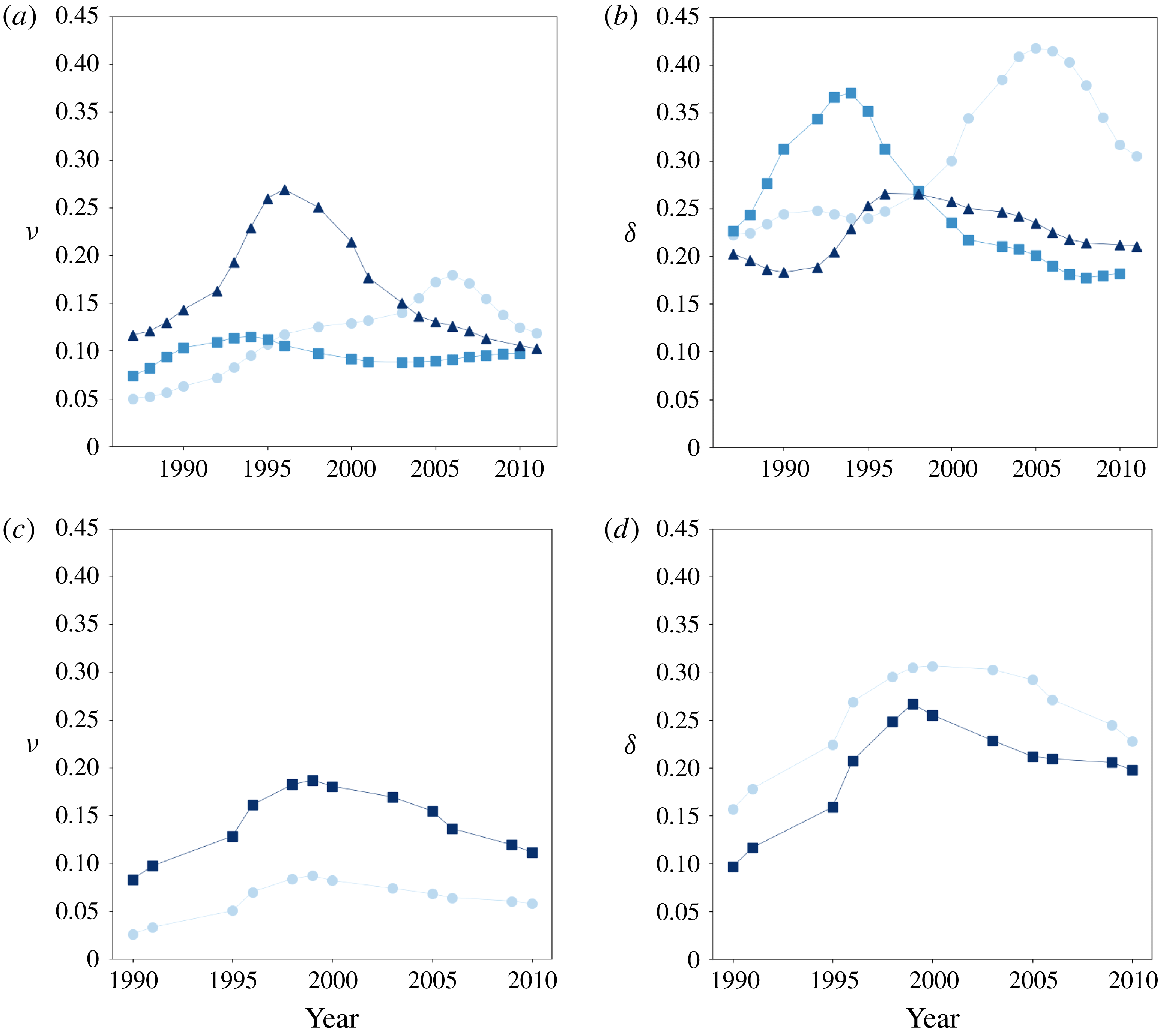
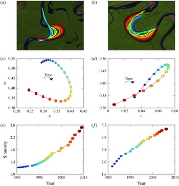
Figure 12 illustrates the coevolution in time of the parameters
 $\unicode[STIX]{x1D708}$
and
 $\unicode[STIX]{x1D6FF}$
in individual bends of the Rio Beni and Rio Ucayali during the observation periods (1985–2011 Rio Beni, 1990–2010 Rio Ucayali). The observed trajectories are consistent with those predicted by the model (see figures 5
b,d and 6
b,d) and both exhibit a two-stage behaviour characterized by a sharper growth in the initial stage followed by a gentler decreasing stage.
We note that, as the stage of development differs from bend to bend, the parameters
 $\unicode[STIX]{x1D708}$
and
 $\unicode[STIX]{x1D6FF}$
do not necessarily peak at the same time. However, as curvature starts increasing, each bend follows an analogous trajectory, although with a different intensity.
Evolutionary trajectories of the parameters
 $\unicode[STIX]{x1D708}$
and
 $\unicode[STIX]{x1D6FF}$
in three individual meander bends of the Rio Beni (Bolivian Amazon, panels a,b) and in two individual meander bends of the Rio Ucayali (Peruvian Amazon, panels c,d).

Evolutionary dynamics of width oscillation and curvature along an individual meander bend of the Rio Beni (Bolivian Amazon, left panels) and one of the Rio Ucayali (Peruvian Amazon, right panels). (a,b) Multi-temporal positions of the channel centreline of Rio Beni (a) and Rio Ucayali (b). Temporal spacing between subsequent centrelines is 1–2 years. The underlying images are a 2015 Landsat false colour composites. (c,d) Observed temporal relationship between curvature ratio
 $\unicode[STIX]{x1D708}$
and amplitude of width oscillation
 $\unicode[STIX]{x1D6FF}$
of Rio Beni (a) and Rio Ucayali (b). (e,f) Time growth of sinuosity of Rio Beni (a) and Rio Ucayali (b). The coloured marks represent the legend for panels (a–d).

Reach-averaged evolution of meander bends of two large rivers from the Amazon basin extracted from three decades of Landsat images (1985–2015) of a 400 km reach (Rio Beni) and of a 900 km reach (Rio Ucayali). Box plots of bend-scale values of: (a) curvature ratio
 $\unicode[STIX]{x1D708}$
, Rio Beni (Bolivian Amazon); (b) width oscillations
 $\unicode[STIX]{x1D6FF}$
, Rio Beni; (c) curvature ratio
 $\unicode[STIX]{x1D708}$
, Rio Ucayali (Peruvian Amazon); (d) width oscillations
 $\unicode[STIX]{x1D6FF}$
, Rio Ucayali. The upper and lower limits of boxes correspond to the 84th and 16th percentiles, respectively, with vertical lines extending to the 95th and 5th percentiles of the category. The percentage of bends, within the examined reach and the whole set of images, for each class of sinuosity
 $\unicode[STIX]{x1D70E}$
is reported on top of each box.

Figure 13 illustrates the observed evolution of the centreline of two individual bends along the Rio Beni and the Rio Ucayali and the resulting trajectories on the (
 $\unicode[STIX]{x1D708},\unicode[STIX]{x1D6FF}$
) plane, showing a hysteretic behaviour similar to that predicted by the theoretical model (figure 11), with the maximum curvature lagging behind the peak of
 $\unicode[STIX]{x1D6FF}$
. The figure also shows that sinuosity grows nearly monotonically as the meander bend develops in time. This suggests the possible use of sinuosity as a proxy for time, thus allowing us to use the properties of observed meander bends at different stages of their lifecycle before cutoff for a semi-quantitative comparison with model predictions.
The outcomes are reported in the box plots of figure 14, in terms of the dimensionless parameters
 $\unicode[STIX]{x1D708}$
and
 $\unicode[STIX]{x1D6FF}$
. With the age of individual bends not known a priori, here we use channel sinuosity as a proxy for the evolutionary stage of an individual meander bend between two subsequent cutoffs. Therefore, sinuosity allows us to compare individual bends with a different evolutionary history and to build a statistical analysis over the entire reach and the whole three decades record of Landsat images. Figure 14 can then be interpreted as a portrait of the overall temporal evolution of curvature and width oscillations along the examined reaches of Rio Beni and Rio Ucayali. The resulting median evolutionary trajectories of the parameters
 $\unicode[STIX]{x1D708}$
and
 $\unicode[STIX]{x1D6FF}$
keep the same two-stage behaviour of individual bends reported in figure 12 and are therefore consistent with those predicted by the model. The peak value of curvature occurs when sinuosity is in the range
 $1.6\div 1.8$
. At larger values of sinuosity the curvature ratio
 $\unicode[STIX]{x1D708}$
follows a stage of slight decay, as predicted by the variable width model. On the other hand, after the peak,
 $\unicode[STIX]{x1D6FF}$
-values keep nearly constant in the Rio Ucayali and slightly increase in the Rio Beni, while the model would predict a decreasing stage. Such discrepancy might be related to the paucity of data with large sinuosity, and may also reflect the effect of missing ingredients in the present model. Among them attention should be paid to the allogenic process of differential bank erosion and accretion rates at opposite banks (Eke et al.
Reference Eke, Czapiga, Viparelli, Shimizu, Imran, Sun and Parker2014a
), to floodplain heterogeneity (Güneralp et al.
Reference Güneralp, Abad, Zolezzi and Hooke2012) and to the relevance of the fine fraction of sediments of the investigated rivers (Braudrick et al.
Reference Braudrick, Dietrich, Leverich and Sklar2009).
The predicted upper-bound value of peak curvature,
 $\unicode[STIX]{x1D708}_{max}$
is plotted as a function of the Cartesian wavenumber,
 $\unicode[STIX]{x1D6EC}$
(red line), compared with observed values of curvature ratio,
 $\unicode[STIX]{x1D708}$
, from the whole dataset of Lagasse et al. (Reference Lagasse, Zevenbergen, Spitz, Thorne, Associates and Collins2004). River bends are classified according to Brice (Reference Brice1975).

Finally, hysteresis cycles of figure 11 highlight the weak dependence of the peak value of curvature on flow parameters even in the case of variable width. If we neglect the nonlinear terms in system (3.7) we can readily derive an upper-bound value of curvature which is independent of hydrodynamics. By imposing
 $$\begin{eqnarray}\frac{\text{d}}{\text{d}t}\unicode[STIX]{x1D708}=0,\end{eqnarray}$$
and keeping only the leading terms in (3.7a,c
) we find that peak curvature is reached when the amplitude
 $|\unicode[STIX]{x1D717}_{1}|$
is equal to
 $1/\sqrt{2}$
. Recalling (2.22) we then obtain
 $$\begin{eqnarray}\unicode[STIX]{x1D708}_{max}=\frac{1}{\sqrt{2}}\unicode[STIX]{x1D706}_{max},\end{eqnarray}$$
where
 $\unicode[STIX]{x1D706}_{max}$
is the intrinsic wavenumber corresponding to the maximum curvature, whose relationship with the initial value
 $\unicode[STIX]{x1D706}_{0}$
can be obtained by interpolating the model results. We then find
 $$\begin{eqnarray}\unicode[STIX]{x1D708}_{max}\simeq 0.4\unicode[STIX]{x1D6EC},\end{eqnarray}$$
where
 $\unicode[STIX]{x1D6EC}$
denotes the Cartesian wavenumber (which coincides with
 $\unicode[STIX]{x1D706}_{0}$
). We note that the above formula can be readily obtained from purely geometrical considerations (Yalin Reference Yalin1992). When tested on the whole dataset of Lagasse et al. (Reference Lagasse, Zevenbergen, Spitz, Thorne, Associates and Collins2004), for each river type of Brice’s (Reference Brice1975) classification, equation (5.3) performs quite well, as most of the data fall below the predicted upper bound, and it correctly reproduces the dependence of curvature on the Cartesian length of meanders, as shown in figure 15. Furthermore, the predicted value of sinuosity at peak curvature,
 $\unicode[STIX]{x1D70E}|_{\unicode[STIX]{x1D708}_{max}}\simeq 1.77$
, falls in the range where the largest values of
 $\unicode[STIX]{x1D708}$
are observed, according to the field data of figure 14(a,c).
6 Discussion
The results presented in § 4 suggest that the width ratio falling below or above the resonant value crucially controls the style of planform evolution of meandering channels with spatially oscillating width. Such difference is known to be key in the planform evolution of equiwidth meandering channels (Seminara et al. Reference Seminara, Zolezzi, Tubino and Zardi2001), but it was not pointed out before in relation to variable width meanders.
The main outcome is that super-resonant meanders are more likely to display width oscillations driven by the autogenic mechanism, with a maximum value of their amplitude occurring in the range
 $(\unicode[STIX]{x1D6FD}=\unicode[STIX]{x1D6FD}_{R}\div 2\unicode[STIX]{x1D6FD}_{R})$
and a corresponding phase lag that forces local widening to occur far downstream of the bend apex. In such conditions width variations are found to weaken the planimetric activity of meanders, mainly reducing meander length and floodplain width (figures 7
b and 10).
We now attempt to provide a mechanistic explanation of the behaviour described in § 4. Solution of system (3.7), along with (3.5a–c ), provides us with an in-depth understanding of the adjustment of width oscillation and of the interaction between width and curvature in the planform development of meander bends.
Equations (3.5a,b
) suggest that the evolution of the channel axis is mainly driven by the linear
 $O(\unicode[STIX]{x1D708})$
term. Therefore the lateral migration rate depends on the position along a meander wavelength of the maximum of the excess flow velocity,
 $U_{10}$
, at the bank. Figure 16(a) provides a representative plot of the phase lag of the
 $U_{10}$
solution with respect to curvature distribution as a function of the width ratio and meander wavenumber, for given values of the flow parameters. Because meanders grow when the phase lag falls in the range
 $(-\unicode[STIX]{x03C0}/2\div \unicode[STIX]{x03C0}/2)$
, the figure shows that planform development occurs provided meander wavenumber keeps relatively small, regardless the value of the width ratio. In the
 $(\unicode[STIX]{x1D706},\unicode[STIX]{x1D6FD})$
plane of figure 16(a) the resonant value
 $\unicode[STIX]{x1D6FD}_{R}$
corresponds to the intersection of the marginal stability curve with the curve discriminating upstream from downstream migration.
The phase lag of the
 $O(\unicode[STIX]{x1D708})$
and
 $O(\unicode[STIX]{x1D708}^{2})$
perturbations of longitudinal velocity with respect to curvature distribution in the
 $(\unicode[STIX]{x1D706},\unicode[STIX]{x1D6FD})$
plane, initial values:
 $\unicode[STIX]{x1D703}_{0}=0.1$
and
 $d_{s}=0.01$
. (a) The phase lag of
 $U_{10}$
. (b) The phase lag of
 $U_{20}$
, reprojected on the half-wavelength. The red dashed curve represents the marginal stability curve, separating unstable (meander formation) and stable conditions (meander suppression). The green continuous curve in panel a represents the separation between downstream migrating (mainly sub-resonant) and upstream migrating (mainly super-resonant) meanders.

On the other hand,
 $\unicode[STIX]{x1D6FD}$
controls the direction of propagation of the channel planform, such that lower values of
 $\unicode[STIX]{x1D6FD}$
(mainly sub-resonant) imply downstream migrating meanders, while higher values (mainly super-resonant) correspond to upstream migrating meanders. This is the main cause of the different evolutionary trajectories of meanders reported in figures 5(a) and 6(a). As a meander develops in time its length increases and therefore
 $\unicode[STIX]{x1D706}$
decreases, which implies a change in the phase lag of
 $U_{10}$
. As pointed out in § 4, the increase of channel length is also responsible, through (2.22), for the reduction of curvature ratio
 $\unicode[STIX]{x1D708}$
experienced in the second stage of meander development.
Meander dynamics is also affected by width variations through the nonlinear
 $O(\unicode[STIX]{x1D708}\unicode[STIX]{x1D6FF})$
contribution, which can either promote or inhibit morphological activity depending on the phase lag
 $\unicode[STIX]{x1D713}_{width}$
. According to the stability analysis of Luchi et al. (Reference Luchi, Zolezzi and Tubino2011), when width oscillations are nearly in phase with curvature (wider-at-bends meander,
 $\unicode[STIX]{x1D713}_{width}=0,\unicode[STIX]{x03C0}$
) meander evolution is promoted, while their effect becomes weaker (or even negative at large
 $\unicode[STIX]{x1D6FD}$
) as their peak shifts towards the inflection points (
 $\unicode[STIX]{x1D713}_{width}=\pm \unicode[STIX]{x03C0}/2$
). Figure 9 suggests that the former condition is met when
 $\unicode[STIX]{x1D6FD}$
is far from the resonant range, while the latter condition characterizes near resonant and super-resonant meanders, which may be the cause of the observed reduction of channel sinuosity reported in figure 7(b).
Equation (3.5c
) highlights how forcing and suppressing terms interact in the formation of width oscillations. In this case a forcing effect is required to promote width variations because the linear
 $O(\unicode[STIX]{x1D6FF})$
contribution invariably produces a stabilizing effect. As an initially equiwidth, quasi-straight river with a weak periodic perturbation of its centreline curvature starts developing, curvature self-forces its own growth but also forces the width distribution to vary longitudinally due to nonlinear autogenic
 $O(\unicode[STIX]{x1D708}^{2})$
effect. Therefore, the amplitude of width variations experiences a relatively fast growth in the initial stage of development due to the increase of the curvature ratio. However, increasing values of
 $\unicode[STIX]{x1D6FF}$
imply an increasing role of the
 $O(\unicode[STIX]{x1D6FF})$
contribution. When these two contributions balance one another, a peak is reached, and then the magnitude of the linear
 $\unicode[STIX]{x1D6FF}$
term becomes dominant and a decreasing stage is observed, enforced by the decline of curvature.
The above discussion clarifies the role of the nonlinear
 $O(\unicode[STIX]{x1D708}^{2})$
solution as the main agent able to produce autogenic width variations. As this solution attains its maximum value within the resonant range, one could expect a corresponding maximum response of width oscillations in the same range. A glance at figure 8 suggests that this is not the case, because the maximum value of
 $\unicode[STIX]{x1D6FF}$
consistently occurs for larger values of
 $\unicode[STIX]{x1D6FD}$
, say
 $\unicode[STIX]{x1D6FD}\simeq 1.5\unicode[STIX]{x1D6FD}_{R}$
.
The reason for this unexpected behaviour is related to the change of position of width maximum with respect to curvature distribution, the phase lag
 $\unicode[STIX]{x1D713}_{width}$
, experienced as the length of meander develops in time. If
 $\unicode[STIX]{x1D713}_{width}$
is relatively stable in time, the amplitude
 $\unicode[STIX]{x1D6FF}$
of width variations is enforced, because the
 $O(\unicode[STIX]{x1D708}^{2})$
contribution continuously acts at nearly the same position along the meander wavelength (e.g. figure 5
c), while the growth of
 $\unicode[STIX]{x1D6FF}$
is weaker when the phase lag continuously shifts through the meander over time. Through (3.5c
) the phase lag of width variations is driven by the phase of the
 $U_{20}$
component, which is reported in figure 16(b) in the
 $(\unicode[STIX]{x1D706},\unicode[STIX]{x1D6FD})$
plane, for given values of the flow parameters, re-projected on half-wavelength. In this plane meander trajectory in time corresponds to a shift of the intrinsic wavenumber
 $\unicode[STIX]{x1D706}$
from its initial value to smaller values as sinuosity increases. Therefore, the phase of the
 $U_{20}$
component experiences a strong variation as the meander develops in time except for a range of values of
 $\unicode[STIX]{x1D6FD}$
(
 $\unicode[STIX]{x1D6FD}\simeq 22{-}25$
in figure 16
b) centred around
 $1.5\unicode[STIX]{x1D6FD}_{R}$
, which corresponds to the range where the maximum amplitude of width oscillations is predicted by the model (figure 8). We note that also the flow parameters slowly vary in time as meander develops. However, their variation does not produce, at least qualitatively, any significant change with respect to the scenario reported in figure 16(b).
It is worth recalling that the plots in figure 16 refer to the theoretical outcomes of Seminara & Tubino (Reference Seminara and Tubino1989, Reference Seminara and Tubino1992). Predictions of the phase lag of the perturbation solution at different orders of approximation (
 $O(\unicode[STIX]{x1D708})$
,
 $O(\unicode[STIX]{x1D708}^{2})$
, see figure 16
b) have received experimental and, to some extent, field validation in a series of previously published studies, thus providing further support to the above reasoning. More specifically, the experiments of Colombini, Tubino & Whiting (Reference Colombini, Tubino, Whiting, Wiley and Ltd.1992) have shown a decreasing tendency of the phase lag of the
 $O(\unicode[STIX]{x1D708})$
solution with the width ratio
 $\unicode[STIX]{x1D6FD}$
at constant wavenumber
 $\unicode[STIX]{x1D706}$
, while the phase lag invariably increases with
 $\unicode[STIX]{x1D706}$
for constant
 $\unicode[STIX]{x1D6FD}$
, for
 $\unicode[STIX]{x1D6FD}$
in the range 12–20 and for
 $\unicode[STIX]{x1D706}$
in the range 0.15–0.3. These trends are well reproduced by the
 $O(\unicode[STIX]{x1D708})$
solution, as reported in Zolezzi (Reference Zolezzi2000) (see supplementary material available online at https://doi.org/10.1017/jfm.2019.574). Testing the behaviour of the
 $O(\unicode[STIX]{x1D708}^{2})$
phase lag in the parameter space with experimental data is less obvious; however, the work of Luchi et al. (Reference Luchi, Hooke, Zolezzi and Bertoldi2010a
) and the review of Zolezzi, Bertoldi & Tubino (Reference Zolezzi, Bertoldi and Tubino2012a
) have reported two applications of the
 $O(\unicode[STIX]{x1D708}^{2})$
solution to field cases, showing a reasonable agreement with the observed location of mid-channel bars in the meandering River Dane and River Dean in the UK. Besides the phase lag, outcomes of the same perturbation approach have been further validated by Seminara & Tubino (Reference Seminara and Tubino1992) for the amplitude and the phase lag of the complete nonlinear solution. Furthermore, Luchi et al. (Reference Luchi, Zolezzi and Tubino2010b
) have shown good agreement between theoretical predictions and experimental observations of Colombini et al. (Reference Colombini, Tubino, Whiting, Wiley and Ltd.1992) for the amplitude of the
 $O(\unicode[STIX]{x1D708}^{2})$
solution, while semi-quantitative comparisons of the phase lag of the
 $O(\unicode[STIX]{x1D708}^{2})$
solution with two field cases has been reported by Luchi et al. (Reference Luchi, Zolezzi and Tubino2011) and by Zolezzi et al. (Reference Zolezzi, Bertoldi and Tubino2012a
).
7 Conclusions
We investigated the coevolution of channel curvature and curvature-induced (‘autogenic’) channel width oscillations during the planform development of sine-generated meandering rivers through an analytical predictive approach.
This represents an important advance in analytical modelling of meander planform evolution which so far has been mostly based on channel curvature as the only planform descriptor. The model provides the first mathematical formulation of the planform development of meandering rivers with variable width by extending the analytical formulation proposed by Seminara et al. (Reference Seminara, Zolezzi, Tubino and Zardi2001) for the constant width case, through the application of the classical lateral migration laws to each bank, instead of the centreline. The analytical treatment allows for a clear identification of the distinct contributions of curvature and width variations to flow field, sediment transport and planform evolution process, that account for the linear responses to channel curvature and width oscillations
 $O(\unicode[STIX]{x1D708}),O(\unicode[STIX]{x1D6FF})$
, for autogenic width oscillations nonlinearly forced by curvature
 $O(\unicode[STIX]{x1D708}^{2})$
and for the nonlinear effect of width oscillations on curvature development
 $O(\unicode[STIX]{x1D708}\unicode[STIX]{x1D6FF})$
.
The proposed approach successfully reproduces the evolutionary behaviour as it emerges from data newly extracted from two large meandering rivers freely evolving in the Amazon basin. We identify curvature nonlinearity as the forcing function for the formation and growth of oscillations of the channel width, which then undergoes a self-dampening linear mechanism. This regulates their amplitude
 $\unicode[STIX]{x1D6FF}$
, which is fundamentally controlled by the channel aspect ratio as for linear, equiwidth meanders. The predicted
 $\unicode[STIX]{x1D6FF}$
-values are consistent with data from Lagasse et al. (Reference Lagasse, Zevenbergen, Spitz, Thorne, Associates and Collins2004). The theory confirms the distinction between sub- and super-resonant meanders as a key feature of meander evolution, since the resonant channel aspect ratio (Blondeaux & Seminara Reference Blondeaux and Seminara1985) discriminates between the former, nearly equiwidth meanders, and the latter, having larger width oscillations. The role of width variations is not overwhelming for sub-resonant meanders, while it is important in the super-resonant context, whereby meander sinuosity is suppressed and fattening/skewing effects are enhanced.
An interesting information is related to the effect of channel width oscillations on the predicted amplitude of the meander belt: the floodplain width occupied by super-resonant meandering rivers is reduced by a factor 2 compared to equiwidth meanders, as a consequence of the reduction of meander sinuosity driven by width oscillations. Conversely, width oscillations do not seem to significantly affect the floodplain width occupied by sub-resonant meandering rivers.
A natural follow up of the present work is the inclusion of the ‘allogenic’ width oscillations, due to different rates of erosion and accretion at opposite banks.
Acknowledgements
This work is supported by the Italian Ministry of Education, University and Research (MIUR) in the frame of the ‘Departments of Excellence’ grant L. 232/2016, by the ‘Agenzia Provinciale per le Risorse Idriche e l’Energia’ (APRIE) of the Province of Trento (Italy) and has been (partially) carried out within the SMART Joint Doctorate (Science for the MAnagement of Rivers and their Tidal systems) funded with the support of the Erasmus Mundus programme of the European Union.
Supplementary material
Supplementary material is available at https://doi.org/10.1017/jfm.2019.574.