1. Introduction
Stratified gas–liquid flow through pipes has been studied extensively in the past due to its common occurrence in the (petro)chemical, nuclear, food and other industries. Experimental studies of stratified flow focus on understanding the flow phenomena and gathering data that can be used to build accurate models to predict the flow in the various industrial applications.
In a horizontal pipe, the stratified flow region occupies a large area in the flow pattern map with transition to slug flow for increasing liquid flow rate and to annular flow for increasing gas flow rate. The stratified regime is divided into a smooth stratified region and a wavy stratified region, and the wavy region is divided into subregimes according to the wave type. The division into subregimes adopted here is similar to the one used by Espedal (Reference Espedal1998) and by Fernandino & Ytrehus (Reference Fernandino and Ytrehus2006) and it distinguishes between the following wave types: (i) small-amplitude 2D waves, (ii) small-amplitude 3D waves, (iii) large-amplitude 2D waves and (iv) large-amplitude 3D waves.
Small-amplitude (SA) 2D waves occur when both the gas and liquid flow rates are low. These waves appear very uniform, and the wave profile remains largely stationary. The wavelength ranges between 1 and 4 cm (for air/water at atmospheric conditions); the wave height is typically less than 2 mm (Andritsos & Hanratty Reference Andritsos and Hanratty1987; Bontozoglou & Hanratty Reference Bontozoglou and Hanratty1990). Small-amplitude 3D waves occur when the liquid flow rate is increased. The wave profile is unsteady, and these waves thus appear much less uniform than 2D SA waves. Large-amplitude (LA) 2D waves appear when the liquid flow rate is increased even further. The wave pattern is more uniform and stationary, with long waves (2–3 times longer than in the previous wave patterns) with higher amplitude, which reaches a maximum at the pipe wall (Strand Reference Strand1993; Fernandino & Ytrehus Reference Fernandino and Ytrehus2006). Finally, 3D LA waves occur at high gas flow rates, with substantial liquid flow rates. These are usually referred to as ‘roll waves’, since they are characterised by the appearance of solitary wave-like structures that are seemingly dragged by the gas flow across the underlying liquid layer.
Further insight into the physics of stratified flow, and in particular the relation between the waves and the underlying flow, can be obtained by measuring not only the bulk flow properties and wave characteristics but also the velocities of the liquid layer. Unfortunately, very few studies that report such measurements exist; some of the first to perform these measurements were Paras & Karabelas (Reference Paras and Karabelas1992) and Strand (Reference Strand1993). Recently, measurements were performed by Vestøl & Melaaen (Reference Vestøl and Melaaen2007) using particle image velocimetry (PIV). Although these studies provided us with more insight, they were limited to turbulent conditions. Laminar and transitional conditions were not reached – despite being relevant for flows of liquids with higher viscosity – possibly because this required measuring in very thin liquid layers, which has proven to be very difficult (Paras & Karabelas Reference Paras and Karabelas1992; Vestøl & Melaaen Reference Vestøl and Melaaen2007).
In our recent study (Birvalski et al. Reference Birvalski, Tummers, Delfos and Henkes2014), a velocity measurement technique for very thin liquid layers was successfully developed. We studied selected cases within the 2D SA and 3D SA wave pattern regions, and showed that the 2D SA cases have a laminar liquid layer, while the 3D SA cases have a turbulent liquid layer. Besides this, the velocities and the wave characteristics were analysed by comparing with previous measurements and with wave theory. The objective of this study is to continue this investigation by determining (i) where the transition from laminar to turbulent flow occurs, (ii) where the change from 2D SA to 3D SA waves occurs and (iii) whether there is any interaction between the two phenomena. In particular, it is of interest to investigate whether the transition to turbulence is driven purely by the shear at the liquid–wall interface or whether it is also enhanced/suppressed by the shear at the (smooth or wavy) gas–liquid interface. Furthermore, it is of interest to investigate which mechanism is responsible for the observed change from the 2D SA to the 3D SA wave pattern, and whether this mechanism is influenced by the turbulence in the liquid layer.
These questions are approached in the present study by measuring at a large number of points in the transitional region, i.e. in the part of the flowmap where transition from laminar to turbulent flow and from 2D SA to 3D SA wave patterns occurs. The same experimental set-up and measurement technique as in our previous study were used. The results obtained in this way are expected to increase our understanding of stratified flow, especially in the low-Reynolds-number region, and thereby lead to the improvement of models for gas–liquid transport through pipelines.
2. Experimental set-up
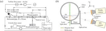
A horizontal transparent pipe of 50 mm inner diameter and 10.3 m length was assembled from shorter segments made of PMMA and high-quality glass (see figure 1 a). Air and water at ambient pressure and temperature entered the pipe through a Y-shaped inlet section. The flow then developed over a length of 7.5 m (150 diameters) before it reached the test section. The test section was followed by another 2.5 m of pipe that discharged freely into an open container. The fluids were circulated using a frequency-controlled pump and a fan, and the flow rates were measured using a Coriolis mass flow meter and a turbine volumetric flow meter for the water and air respectively. The temperatures of both fluids were measured at the end of the pipe.
Schematic view of (a) the experimental set-up and (b) the test section. Indications
 $p$
and
 $T$
in (a) stand for pressure and temperature, respectively.

The PIV and the profile detection system consisted of two CCD cameras (PCO Sensicam qe and PCO Sensicam) that were positioned slightly below (above) the interface and angled up (down) to image the particles in the liquid layer and the interface respectively (see figure 1
b). Both cameras were equipped with 100 mm lenses (Tokina,
 $100~\text{mm}/2.8$
macro) and longpass filters (Hoya O56). The field of view (FOV) was
 ${\sim}26\times 20~\text{mm}^{2}$
for the PIV camera and
 ${\sim}28\times 22~\text{mm}^{2}$
for the profile camera.
The light source was a Continuum Minilite double pulsed PIV laser (Nd:YAG, 532 nm), used in low-power mode (approximately
 $1.2~\text{mJ}~\text{pulse}^{-1}$
) at a frequency of 2 Hz. The reflections from the pipe wall and from the interface necessitated the use of fluorescent seeding particles from a fluorescent acrylic paint (Lefranc & Bourgeois, Flashe Vinyl, fluorescent light orange colour). The light emitted by the particles passed through the longpass filters, while the laser light was blocked. The light beam was shaped into an
 ${\sim}35~\text{mm}$
wide and
 ${\sim}0.5~\text{mm}$
thick sheet that was directed into the liquid layer through the bottom pipe wall. The sheet was vertical and contained the pipe axis.
The cameras were calibrated by imaging a square grid of dots (0.5 mm diameter and 1 mm apart) positioned in the plane of the light sheet. LaVision’s Davis 8 software was used to dewarp and calibrate the raw images, resulting in a common real-world coordinate system for both cameras.
2.1. Measurement conditions
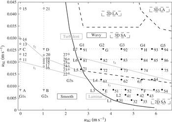
Data were collected in 17 flow conditions in the smooth region (labelled 11–27, see figure 2) and 29 flow conditions in the wavy region (labelled 31–94). In figure 2, new measurements are presented alongside the measurements from Birvalski et al. (Reference Birvalski, Tummers, Delfos and Henkes2014), which are labelled A–H. For every flow condition, 2000 double-frame images were recorded by both the profile and the PIV camera.
Experimental flowmap. Cases without waves are marked with open symbols and those with waves with solid symbols. New cases are marked with circles and those of our previous study (Birvalski et al.
Reference Birvalski, Tummers, Delfos and Henkes2014) with triangles. Dotted lines G1s–G3s, G1–G5 and L1–L7 are used for reference in the text throughout this study. Regions of smooth, 2D SA, 3D SA, 2D LA and 3D LA waves are also shown, separated by dashed lines. The line separating the smooth from the wavy region is an experimental result of Barnea, Shoham & Taitel (Reference Barnea, Shoham and Taitel1982). Measurement points E, G, 31, 41, 42 and 52 are considered part of lines G2–G4 when the data are presented. Lines
 $\text{t}_{1}{-}\text{t}_{4}$
represent the approximate boundaries of the laminar, transitional and turbulent regions of the liquid phase, determined in § 4.1. Here, superficial gas velocity,
 $u_{SG}$
is plotted against the superficial liquid velocity,
 $u_{SL}$
.

In smooth flow, measurements were performed along lines of constant superficial gas velocity (G1s–G3s, where ‘G’ stands for ‘gas’) to determine the boundaries of the laminar–turbulent transition. For the same reason, the data in the wavy region covered the region between cases E and F (laminar) and G and H (turbulent). At high values of the superficial gas velocity (
 ${>}6~\text{m}~\text{s}^{-1}$
) the interface becomes increasingly intermittent. The gas flow rate in our measurements was increased until this effect was not overly pronounced.
The measurement points and the observed wave pattern transition boundaries are shown in figure 2. The transition boundaries represent a region of finite width in which the change of the wave pattern occurs.
3. Data reduction and processing
Imaging of the liquid layer beneath an air/water interface is characterised by the appearance of ghost particle images (see, e.g., Peirson Reference Peirson1997; Law, Khoo & Chew Reference Law, Khoo and Chew1999). Due to the interface acting as a mirror, every real particle image also has a reflection on the other side of the surface. The position of the interface in the PIV images, however, is difficult to detect using a computer algorithm, although the interface is visible to the eye. Therefore, the profile camera is used to record the surface from above the liquid layer. These images are processed to extract the interfacial profile. The profile is subsequently used to generate a mask for every individual velocity field (resulting from PIV processing), thereby correctly setting the top boundary of the flow.
The processing steps performed to derive results from the raw (PIV and profile) images are described in the following sections.
3.1. Profile detection and PIV processing
When observed with the profile camera, the liquid layer appears as a bright region, where the top edge is the interfacial profile, which was detected in a way similar to that of Mukto, Atmane & Loewen (Reference Mukto, Atmane and Loewen2007) and Siddiqui & Loewen (Reference Siddiqui and Loewen2007) in wind-wave tanks. Specific to our geometry is the occasional occurrence of spurious reflections from the top pipe wall (see figure 1 b). The detection algorithm was designed to correct for these erroneous reflections.
The edge detection algorithm first applies a Sobel filter (
 $3~\text{pixel}\times 3~\text{pixel}$
in size), followed by a Wiener smoothing filter (
 $11~\text{pixel}\times 11~\text{pixel}$
in size), and then thresholds the image. The resulting interfacial profile is further processed by performing morphological operations (opening and closing, typically in 1–3 steps, see, e.g., Gonzales, Woods & Eddins Reference Gonzales, Woods and Eddins2009) to eliminate the erroneous detections arising from the spurious light reflected from the top wall. Finally, linear averaging filters are applied to make the profile smooth and continuous. The quality of edge detection is visually inspected by overlaying the detected profile on the corresponding PIV image. The accuracy of interface detection is estimated to be approximately 5 pixels (0.1 mm).
The PIV processing was performed using LaVision’s Davis 8 software. A multipass cross-correlation procedure was applied with a final interrogation area size of
 $16~\text{pixel}\times 16~\text{pixel}$
(
 ${\sim}0.3\times 0.3~\text{mm}$
), with 50 % overlap. Outliers were detected using common techniques (local median filter, correlation peak ratio threshold, etc.) and they were first replaced by higher-order correlation peaks and then by interpolation. Finally, a
 $3\times 3$
vector averaging filter was applied.
The final velocity fields were obtained by masking the velocity fields resulting from PIV processing using the previously detected interfacial profiles.
3.2. Phase averaging
In wavy flows, it is of interest to decompose the velocity field into the mean flow, the wave-induced fluctuations and the turbulence-induced fluctuations (e.g. Hussain & Reynolds Reference Hussain and Reynolds1970). In our study, however, phase averaging was performed to investigate the relationship between the vortical structures and the waves. This was done using a method developed by Siddiqui & Loewen (Reference Siddiqui and Loewen2010) for low-frequency PIV data, like the data collected in the present study.
The method works by detecting the zero crossings, the crests and the troughs, which divides the waves into wave quarters (labelled Q1–Q4, see Birvalski et al.
Reference Birvalski, Tummers, Delfos and Henkes2014). These characteristic points are assigned a phase; zeros are
 $90^{\circ }$
and
 $270^{\circ }$
, crests are
 $0^{\circ }$
and troughs are
 $180^{\circ }$
. The profile segments between the zeros and the crests/troughs are then assigned a phase by linearly dividing the axial distance between these points. Using this technique, waves with wavelengths of up to twice the width of the FOV can be resolved. This amounts to 52 mm in the present study.
Phase averaging can be performed for any phase angle by first extracting the radial (wall-normal) lines of some quantity (velocity, vorticity, swirling strength, etc.) at the particular phase from the corresponding vector or scalar fields, and then by ensemble averaging the extracted lines. In this study, the averaging is performed in the Eulerian coordinate system which has the origin at the pipe wall, with the
 $x$
axis pointing axially in the mean flow direction and the
 $y$
axis pointing radially towards the centre of the pipe.
Further details of the profile detection technique can be found in Birvalski et al. (Reference Birvalski, Tummers, Delfos and Henkes2013) and of the phase averaging procedure in Siddiqui & Loewen (Reference Siddiqui and Loewen2010).
3.3. Quantification of the laminar–turbulent transition
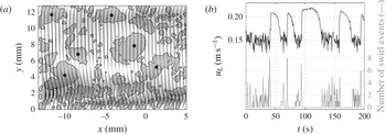
To quantify the laminar–turbulent transition in smooth flows, the turbulence intermittency factor is calculated by extracting the axial velocity from a fixed point located axially in the middle of the FOV and radially just beneath the lowest measured interface position (for a given case). This time signal (an example of which is shown in figure 3
b) has high values (
 ${\sim}0.2~\text{m}~\text{s}^{-1}$
) with low fluctuation in laminar patches and low values (
 ${\sim}0.15~\text{m}~\text{s}^{-1}$
) with high fluctuation in turbulent patches. The signal is thresholded (at
 $0.18{-}0.19~\text{m}~\text{s}^{-1}$
, depending on the absolute velocities in a particular case), after which the intermittency is calculated.
In wavy liquid layers it is not possible to apply the same procedure, since the absolute values of the velocity and of the velocity fluctuations in laminar and turbulent fields within one case do not differ enough (due to wave-induced motion) for the two to be distinguished. Therefore, we used a method that does not separate the two motions, but rather aims at detecting only the turbulent structures within the complete velocity fields.
One of the defining characteristics of turbulence is the presence of vortical structures, and – specifically for wall-bounded turbulence – the presence of hairpin-type vortices organised into hairpin packets (e.g. Adrian, Meinhart & Tomkins Reference Adrian, Meinhart and Tomkins2000b
; Adrian Reference Adrian2007). The intersection between a streamwise wall-normal light sheet with the hairpin packets shows a number of uniform-momentum zones and a number of vortices (Adrian Reference Adrian2007). These vortices can be detected and quantified in a number of ways (see, e.g., Adrian, Christensen & Liu Reference Adrian, Christensen and Liu2000a
; Chakraborty, Balachandar & Adrian Reference Chakraborty, Balachandar and Adrian2005). One of the widely applied methods is based on the calculation of the discriminant
 ${\it\Delta}$
of the velocity gradient tensor
 $\partial u_{i}/\partial x_{j}$
. When applied to our two-dimensional PIV data, this gives
 $$\begin{eqnarray}{\it\Delta}=\left(\frac{\partial u}{\partial x}+\frac{\partial v}{\partial y}\right)^{2}-4\frac{\partial u}{\partial x}\frac{\partial v}{\partial y}+4\frac{\partial u}{\partial y}\frac{\partial v}{\partial x}.\end{eqnarray}$$
A negative value of the discriminant means that the eigenvalues of the velocity gradient tensor form a complex conjugate pair, which indicates the presence of swirling motion at that point (Zhou et al.
Reference Zhou, Adrian, Balachandar and Kendall1999). The strength of the swirling motion is represented by the magnitude of the imaginary part of the complex conjugate pair. This value is called the swirling strength, and it is calculated using
 ${\it\lambda}_{ci}^{2}=-{\it\Delta}/4$
(Zhou et al.
Reference Zhou, Adrian, Balachandar and Kendall1999). The advantage of using the swirling strength for vortex identification (as opposed to, e.g., vorticity) lies in its ability to discriminate against shear, which is important in high-shear boundary layer flows, such as ours.
(a) An instantaneous velocity and swirling strength field from case 17. The top edge of the graph is the interface, while the bottom edge is the pipe wall. The graph shows the fluctuating velocity field (every third vector in the horizontal direction). The swirling strength field is processed to detect only the largest swirling events, marked with dots. (b) Time traces of the axial velocity and swirl events for the same case (the first 200 s). The axial velocity
 $u_{L}$
is sampled at a point slightly below the minimum interfacial level.

Figure 3(a) shows an instantaneous velocity field and the corresponding swirling strength field from case 17. As is shown, a raw swirling strength field is made up of many connected areas of varying size and intensity. However, not all of the connected structures are vortices that are part of a larger turbulent event. The PIV results always contain a small random error, which produces small areas of swirl (see figure 3 a) that also exist in fully laminar velocity fields (not shown). They are eliminated by applying a filter that discriminates based on the size of the event, using the following approach.
The instantaneous fields are first eroded (e.g. Gonzales et al.
Reference Gonzales, Woods and Eddins2009) by using a circular structuring element. The resulting field is then taken as a marker in a reconstruction procedure in which the initial field is the mask (Gonzales et al.
Reference Gonzales, Woods and Eddins2009). The structuring element is circular,
 ${\sim}1.4~\text{mm}$
in diameter. In smooth cases – used here to validate the swirling strength as a reliable turbulence indicator – only one filter size (
 ${\sim}1.4~\text{mm}$
) was needed to obtain correct results in all of the cases. Likewise, for the wavy cases, a structuring element of
 ${\sim}1.1~\text{mm}$
was applied. Here, the height of the liquid layer is typically lower, which results in smaller vortices, and therefore requires a smaller filter. Furthermore, the wavy cases were processed with filters ranging in size from
 ${\sim}0.8~\text{mm}$
to
 ${\sim}1.7~\text{mm}$
in diameter, which gave results that remained qualitatively the same.
The ability of the method to discriminate between laminar and turbulent velocity fields is illustrated in figure 3(b). Here, a time trace segment (200 s long) of the axial velocity at a position slightly below the interface for (the smooth and transitional) case 17 is shown along with the number of swirling events detected in the vector fields. The laminar patches contain no swirling events. The turbulent patches, on the other hand, contain as many as eight swirl events per vector field.
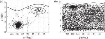
The swirl event method of detecting turbulence is now applied to wavy flows. Here, it is of interest to record not only the number of events per velocity field, but also their position with respect to the phase of the waves. Cases 31 and 82 were processed in this way, and the results are presented in figure 4.
The laminar case 31 with very low liquid and gas velocities has only a few vortices detected away from the single region of high concentration at phase angles of
 ${\sim}150^{\circ }{-}200^{\circ }$
, and at
 ${\sim}0.8{-}2~\text{mm}$
from the wall (region R1, figure 4
a). These vortices are not the result of turbulence, but of the waves, i.e. of wave-induced motion making the third term in (3.1) negative. The vortices detected away from the trough region in case 31 have two sources. The group of vortices with a phase angle of
 $0^{\circ }$
in the trough to crest region (at
 ${\sim}4~\text{mm}$
height, R2 in figure 4
a) appears to also be caused by waves. Here, the axial velocity profile occasionally has a negative vertical gradient, which combines with the positive gradient of radial velocity to produce swirl. The remainder of the swirling events outside the trough have a source that is presently unknown. Their number is very small (
 $O(50)$
structures in
 $O(5000)$
waves in lines L1 and L2), and they are reminiscent of structures detected by Huang et al. (Reference Huang, Hwung, Hsiao and Chang2010) in shoaling waves. Furthermore, they appear to originate at the interface, so we consider these vortices as belonging to the wavy motion and not to the wall-induced turbulence.
Measured phase dependence of the detected swirling events for (a) case 31 and (b) case 82 (crosses). The average interfacial profiles are shown for reference (solid line). Here, wave phase,
 ${\it\varphi}$
is plotted against the liquid height,
 $y$
.

The turbulent case 82, shown in the right graph of figure 4, has a much more uniform distribution of swirl events than case 31. The concentration of swirl events is also slightly higher under the trough at a height of less than 2 mm, which is attributed to the waves (R4, figure 4 b). The high-concentration region just beneath the interface at the same phase position (R3, figure 4 b) is also due to waves, and is not visible in case 31 because those events were typically smaller than the filter size.
The detection of vortices using the swirling strength is performed here in order to derive a property that can quantify the transition from laminar to turbulent conditions in wavy flows. This means that the detected vortices that do not have a turbulent origin must be excluded from further processing. To make sure that wave-induced swirling events are excluded, only the events below the wave crest (from − 90° to + 90° phase angle) up to a height of 3 mm are counted (this area is marked by dashed rectangles in figure 4). The top border of this region is set arbitrarily at 3 mm to avoid the trough to crest region (i.e. to stay in the bulk of the flow) even for the thinnest liquid layer (case 33). The total number of detected swirling events in this region (in all vector fields of a particular case) is divided by the product of the number of wave quarters belonging to the crest and the detection area (which is equal to 3 mm multiplied by the average crest length). In this way, the swirl event density
 $Sw$
(
 $\text{mm}^{-2}$
) is calculated for every case in the wavy region. The swirl event density
 $Sw$
is a dimensional quantity, and its absolute value varies as a function of the parameters chosen for its calculation (filter size, detection area size and position, etc.). However, we verified for the results obtained using this quantity that the characteristics of individual wavy cases relative to each other stay the same, despite the changing input parameters, such as the filter size.
4. Results
4.1. Laminar–turbulent transition
4.1.1. Smooth stratified flow
The transition to turbulence in smooth stratified flow occurs – when observed in the fixed frame of reference – in the usual intermittent way, with patches of turbulence developing (accompanied by rising liquid level) until rapid laminarisation occurs (along with a corresponding drop in liquid level). The laminar patches then slowly destabilise into turbulence, after which the process repeats itself (see Birvalski et al. (Reference Birvalski, Tummers, Delfos and Henkes2014) and also, e.g., Wygnanski & Champagne (Reference Wygnanski and Champagne1973) for similar behaviour in single-phase pipe flow).
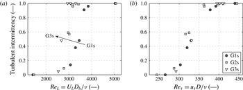
Turbulent intermittency factor of cases along lines G1s–G3s, shown against the Reynolds number based on (a) the bulk liquid velocity (
 $\mathit{Re}_{L}$
) and (b) the friction velocity (
 $\mathit{Re}_{{\it\tau}}$
). The Reynolds number in (a) is determined using the pipe hydraulic diameter
 $D_{h}$
, which is defined as
 $D_{h}=4A_{L}/S_{L}$
, where
 $A_{L}$
is the pipe area occupied by liquid and
 $S_{L}$
is the wetted perimeter. The symbols shown in the legend of (b) are used in both graphs.

The intermittency is calculated for all the smooth cases (11–27, including A–D), and plotted against the Reynolds number for varying superficial gas velocities (G1s–G3s, see figure 5). Figure 5 shows the transition curves for Reynolds numbers defined using the bulk velocity
 $U_{L}$
and the hydraulic diameter
 $D_{h}=4A_{L}/S_{L}$
(where
 $A_{L}$
is the pipe area occupied by liquid and
 $S_{L}$
is the wetted perimeter) and using the wall friction velocity
 $u_{{\it\tau}}$
(obtained by fitting a straight line through the mean velocity profile in the laminar sublayer,
 $y^{+}<5$
) and the pipe diameter
 $D$
as the length scale. Figure 5(a) shows a curve with a typical sigmoid shape that is displaced towards lower values of the Reynolds number as the superficial gas velocity is increased. The
 $\mathit{Re}_{L}$
at which transition starts is
 ${\sim}2500{-}2800$
, ending at
 ${\sim}2900{-}4000$
. This is similar to the values obtained in single-phase pipe flows (see, e.g., Wygnanski & Champagne Reference Wygnanski and Champagne1973; Schlichting Reference Schlichting1979) and in downward-flowing two-phase flow (Lioumbas, Paras & Karabelas Reference Lioumbas, Paras and Karabelas2005).
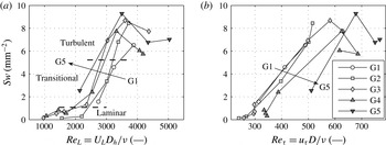
Swirl event density for cases along lines G1–G5 shown against the Reynolds number based on (a) the bulk liquid velocity (
 $\mathit{Re}_{L}$
) and (b) the friction velocity (
 $\mathit{Re}_{{\it\tau}}$
). The Reynolds number in (a) is defined using the pipe hydraulic diameter
 $D_{h}$
, which is defined as
 $D_{h}=4A_{L}/S_{L}$
, where
 $A_{L}$
is the pipe area occupied by liquid and
 $S_{L}$
is the wetted perimeter. The swirl event density in all graphs is multiplied by
 $10^{3}$
. The symbols shown in the legend of (b) are used in both graphs.

Another interesting property of the transition in smooth flows is shown in figure 5(b), where the Reynolds number is defined using
 $u_{{\it\tau}}$
. The transition to turbulence occurs in a narrow range of
 $\mathit{Re}_{{\it\tau}}$
, and at practically the same value of
 $u_{L}$
(not shown), for all the cases from G1s–G3s. This means that the main effect of the air flow on transition – in the range of flow conditions studied – is to reduce the mean liquid height
 $h_{L}$
(i.e. the holdup), while the liquid velocity of transition remains almost constant.
In figure 2, lines
 $\text{t}_{1}$
and
 $\text{t}_{2}$
mark the approximate positions of the boundaries between the laminar, transitional and turbulent regions, based on figure 5.
4.1.2. Wavy stratified flow
The swirl event density
 $Sw$
is calculated for cases along lines G1–G5 (see figure 2). Figure 6 shows the resulting
 $Sw$
as a function of the two Reynolds numbers considered before. The curves of
 $Sw$
have a shape that resembles that of turbulent intermittency curves, presented earlier (figure 5). The typical
 $Sw$
value for a turbulent case is approximately 25 times larger than for a laminar case. The curves can be approximately divided into the laminar, transitional and turbulent sections (see figure 6
a). The bottom border is placed just above the group of cases that have the lowest
 $Sw$
values, and similarly the top border is placed just beneath what is perceived as a group of cases with high
 $Sw$
values. Looking now at figure 6(a), where the
 $Sw$
is shown against the Reynolds number based upon the bulk velocity (
 $\mathit{Re}_{L}$
), we see the same behaviour as in figure 5(a), namely that the transition to turbulence occurs at a lower value of the Reynolds number as the superficial gas velocity increases. When the specific Reynolds numbers at the beginning and the end of the transition are compared in figures 5(a) and 6(a), we can make two observations. First, the
 $\mathit{Re}_{L}$
where the transition begins in figure 6(a) further reduces with increasing
 $u_{SG}$
, following the trend from figure 5(a), e.g.
 $\mathit{Re}_{L}$
in figure 5(a) reduces from
 ${\sim}2800$
(for G1s) to
 ${\sim}2500$
(for G3s), and this continues in figure 6(a) with values going from
 ${\sim}2500$
(for G1) to
 ${\sim}1500$
(for G5). Second, the point where the transition ends – although still reducing with increasing gas flow rate – does not continue the trend measured in G1s–G3s, but occurs at higher values of the Reynolds number, e.g. the transition for G3s ends at
 $\mathit{Re}_{L}\sim 2900$
, while this value is
 ${\sim}3500$
for G1. If we compare figure 6(b) with figure 5(b), where Reynolds numbers based on the friction velocity at the wall are shown, it is observed that the transition for lines G1–G3 occurs at the same values of
 $\mathit{Re}_{{\it\tau}}$
as for lines G1s–G3s in the smooth regime, i.e. the transition begins at
 $\mathit{Re}_{{\it\tau}}\sim 275$
and ends at
 $\mathit{Re}_{{\it\tau}}\sim 400$
. However, it occurs at substantially higher values for lines G4 and G5.
These observations suggest that the presence of waves on the interface, in general, delays both the beginning (for cases G4 and G5) and the end of the transition process. The initial turbulent events (i.e. the laminar-transitional boundary), on the other hand, occur at the expected values of
 $\mathit{Re}_{L}$
, which reduce continuously from the values in the smooth region (for cases G1–G3).
The approximate transition boundaries are presented in the flowmap in figure 2 (
 $\text{t}_{3}$
and
 $\text{t}_{4}$
). Figure 2 also shows the areas where either 2D SA or 3D SA waves were visually observed, separated by a dashed line.
4.2. Wave regime transition
The profile detection and phase averaging procedures result in the average wave height
 $H$
(mm) and wavelength
 ${\it\lambda}$
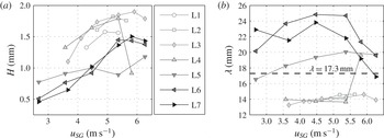
(mm). These quantities are calculated for all of the wavy cases along the constant liquid flow rate lines L1–L7, and the results are shown in figure 7. The wavelengths appear to form two groups, which correspond to the two observed wave patterns. The first group (labelled 2D SA waves), with short wavelengths (
 ${<}15~\text{mm}$
) that differ very little between the cases, is formed by lines L1–L4 (without case 64), and the second group (labelled 3D SA waves), with longer wavelengths (
 ${\sim}17{-}25~\text{mm}$
), is formed by lines L5–L7 (including case 64). In figure 7(a), we see that 2D SA cases have a somewhat larger wave height in comparison to the cases from the 3D SA group. The wavelength of 3D SA waves, and specifically of lines L6 and L7, decreases slightly with increasing gas flow rate, in accordance with the findings of Andritsos & Hanratty (Reference Andritsos and Hanratty1987).
Measured wave height
 $H$
(a) and wavelength
 ${\it\lambda}$
(b) plotted against superficial gas velocity,
 $u_{SG}$
, for cases along lines L1–L7. The dashed line at
 ${\it\lambda}=17.3~\text{mm}$
is the approximate wavelength that separates the capillary- from the gravity-branch solutions, according to linear wave theory (see below, figure 8
b).

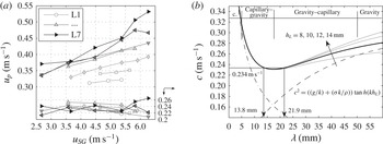
(a) Measured profile velocity
 $u_{p}$
against superficial gas velocity,
 $u_{SG}$
and wave celerity
 $c$
against wavelength,
 ${\it\lambda}$
for cases along lines L1–L7. The wave celerity
 $c$
was obtained by subtracting the bulk liquid velocity
 $U_{L}$
from the profile velocity
 $u_{p}$
. (b) The dispersion relationship, as given by linear wave theory, for air/water flow with
 $h_{L}=8{-}14~\text{mm}$
(solid lines). The dashed line is the contribution of gravity and the dash-dot line is the contribution of surface tension when
 $h_{L}=10~\text{mm}$
(thick black line). For the same liquid height and
 $c=0.234~\text{m}~\text{s}^{-1}$
, two wavelength solutions are produced – 13.8 mm and 21.9 mm – which stem from the capillary and gravity branches of the dispersion relation respectively.

Cases E–H were considered in Birvalski et al. (Reference Birvalski, Tummers, Delfos and Henkes2014), where it was observed that there is a substantial difference in wavelength and in visual appearance between cases E and F (belonging to L3) on one hand, and cases G and H (belonging to L7) on the other hand. However, it was not known where exactly in the flowmap this change occurs, or whether it is gradual or abrupt. The new measurements show that the change is indeed quite steep, which means that the flowmap can be divided into the 2D SA and 3D SA regions, as is shown in figure 2 (dashed line). This study shows that all of the other properties that characterise cases E–H, e.g. the higher steepness and greater asymmetry (i.e. deviation from a sinusoidal profile) of cases E and F in comparison to cases G and H, extend to all of the cases that are part of the corresponding wave pattern regions.
The current experimental set-up also provides measurements of the profile velocity
 $u_{p}$
and of the wave celerity
 $c$
, and these quantities are presented in figure 8 (along L1–L7, (a)). The wave celerity is calculated by subtracting the bulk flow velocity
 $U_{L}$
from the profile velocity
 $u_{p}$
. The profile velocity is in turn obtained by cross-correlating the two profile frames in the horizontal direction and then dividing the displacement by the time separation between the frames. As shown in figure 8
a,
 $u_{p}$
increases as both the superficial gas and liquid velocities increase. The wave celerity, however, stays practically the same for all of the cases measured. This value of
 $c$
is approximately
 $0.23~\text{m}~\text{s}^{-1}$
, which is also the minimum wave celerity predicted by linear (Airy) wave theory (e.g. Dean & Dalrymple Reference Dean and Dalrymple1998) for air/water flows. Despite its simplifications, the linear wave theory was shown (see Birvalski et al.
Reference Birvalski, Tummers, Delfos and Henkes2014) to correctly predict the wave celerity if the wavelength is known (along with the mean liquid height
 $h_{L}$
), and vice versa. It accounts for both surface tension and gravity acting on the interface as forces of restitution. This results in a dispersion relationship that has a characteristic minimum at
 $c\sim 0.23~\text{m}~\text{s}^{-1}$
and
 ${\it\lambda}\sim 17.3~\text{mm}$
(for air/water flow, with water 10 mm high). The dispersion relationship with these input parameters is shown in figure (8
b).
Looking now again at figure 7(b), where a horizontal line is placed at
 ${\it\lambda}=17.3~\text{mm}$
, and keeping in mind that
 $c\sim 0.23~\text{m}~\text{s}^{-1}$
for all of the cases (figure 8), it is seen that the 2D SA cases are in fact capillary–gravity waves (
 ${\it\lambda}\sim 14~\text{mm}$
) and 3D SA cases are gravity–capillary waves (
 ${\it\lambda}\sim 22~\text{mm}$
). Furthermore, since the 2D SA waves have
 ${\it\lambda}\sim 14~\text{mm}$
and the 3D SA waves have
 ${\it\lambda}\sim 22~\text{mm}$
, it seems plausible that the transition from one to the other occurs through a period doubling (
 $2\rightarrow 1$
) bifurcation (see Janssen Reference Janssen1986; Bontozoglou & Hanratty Reference Bontozoglou and Hanratty1990), whereby the wavelength theoretically doubles from an initial value of 12.1 to 24.2 mm. In our experiments, the bifurcation appears to be initiated by the laminar to turbulent transition in the liquid (see § 4.3).
As is shown, the linear wave theory provides valuable physical insight by identifying the dominance of the surface tension over the gravity in 2D SA (capillary–gravity) cases and of the gravity over the surface tension in 3D SA (gravity–capillary) cases. To investigate this further, we determine the intensity of the individual restitutive forces in relation to the inertia of the bulk flow, which is a force acting to disrupt the interfacial wave pattern (e.g. Andritsos & Hanratty Reference Andritsos and Hanratty1987; Brocchini & Peregrine Reference Brocchini and Peregrine2001).
The influence of the mean flow on the interfacial phenomena has been studied, amongst others, by Brocchini & Peregrine (Reference Brocchini and Peregrine2001). In their work, a Froude number–Weber number (
 $\mathit{Fr}$
–
 $\mathit{We}$
) diagram that categorises all of the observed mean flow–surface interaction phenomena has been divided into four zones, based on the relative strength of turbulence over surface tension and gravity. For both
 $\mathit{Fr}$
and
 $\mathit{We}$
, a low value (
 ${<}1$
) means that the turbulence can overcome neither the restraining effect of gravity nor that of the surface tension, while the opposite is true when these numbers are high (
 ${>}1$
). The same analysis is applied in our study. We define
 $\mathit{We}$
and
 $\mathit{Fr}$
in a similar way to Brocchini & Peregrine (Reference Brocchini and Peregrine2001):
 $$\begin{eqnarray}\mathit{We}=\frac{{\it\rho}_{L}u_{L}^{2}h_{L}}{2{\it\sigma}},\quad \mathit{Fr}=\frac{u_{L}k}{\sqrt{2gk\tanh (kh_{L})}},\quad \text{where }k=\frac{2{\rm\pi}}{{\it\lambda}}.\end{eqnarray}$$
The relevant length and velocity scales in our flow are the mean flow velocity
 $u_{L}$
and the mean liquid height
 $h_{L}$
. The Weber number compares the inertia (or the kinetic energy) of the mean flow (
 $0.5u_{L}^{2}$
) with the surface tension term (
 ${\it\sigma}/{\it\rho}_{L}h_{L}$
). The Froude number compares the mean flow inertia (
 $0.5u_{L}^{2}$
) with gravity, represented by the celerity of gravity waves in the liquid layer of finite depth (
 $g\tanh (kh_{L})/k$
).
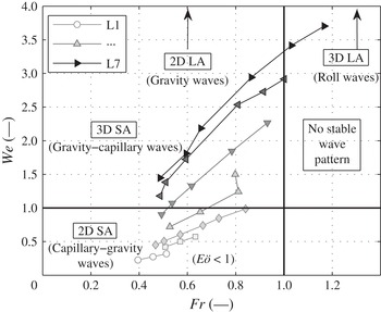
The results are shown in figure 9. The flowmap is divided into four regions, with
 $\mathit{We}=1$
and
 $\mathit{Fr}=1$
as boundaries. Cases along lines L1–L3 belong to the region with
 $\mathit{We}<1$
and
 $\mathit{Fr}<1$
where both surface tension and gravity can overcome the liquid inertia. Which of the two restitutive forces will dominate, and consequently determine the wave characteristics, can be determined by calculating the Eötvös (Bond) number, defined here as
 $E\ddot{o} ={\it\rho}_{L}gH^{2}/{\it\sigma}$
, where
 $H$
is the wave height. The value of
 $E\ddot{o}$
is
 ${\sim}0.2{-}0.5$
, which suggests that the surface tension is dominating gravity, causing the occurrence of capillary–gravity (2D SA) waves in this region. With increasing liquid flow rate (cases along lines L5–L7), turbulence develops and flow inertia increases causing
 $\mathit{We}$
to rise above one, while
 $\mathit{Fr}$
remains below one. Although gravity is now the dominating restoring force, surface tension is still not negligible; therefore, the waves in this region are called gravity–capillary (3D SA) waves. On the other hand, the bulk liquid velocity increases with increasing gas flow rate. When this value becomes larger than the wave celerity (resulting in
 $\mathit{Fr}>1$
), a stable wave pattern can no longer be sustained, as reported earlier (§ 2.1).
Flowmap of the wavy region in
 $\mathit{Fr}{-}\mathit{We}$
coordinates. Regions with different wave patterns are separated by the lines
 $\mathit{Fr}=1$
and
 $\mathit{We}=1$
.

At this point, one can speculate about the remaining wave patterns – namely 2D LA and 3D LA waves – observed in the experiments. Since the 2D LA wave pattern is continuous and the 3D LA pattern is very intermittent, it is expected that the boundary between the two is formed by the line
 $\mathit{Fr}=1$
, which remains to be confirmed in further studies.
The analysis above provides a physical explanation of the transition from 2D SA to 3D SA waves by considering the main forces acting on the interface, without focusing specifically on the laminar–turbulent transition within the bulk liquid flow. Likewise, the transition to turbulence was studied in § 4.1 without giving attention to the interfacial conditions, i.e. to the occurrence of waves or the changing wave patterns. However, the fact that the 2D SA–3D SA wave pattern boundary coincides with the laminar to turbulent transitional region (see figure 2) suggests that one should also look at their mutual interaction.
4.3. Wave–turbulence interaction
As shown in § 4.1, the waves cause the transition to turbulence to occur at a higher value of the Reynolds number than what is expected based on values in the smooth region. In this section, the opposite effect, i.e. the effect of turbulence on the waves, is investigated. This is performed by inspecting the time traces of velocity and interfacial level in selected measurement cases.
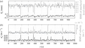
Figure 10 shows the snapshot mean and RMS values of the interfacial level and the axial velocity (determined along a horizontal line at
 ${\sim}0.8~\text{mm}$
from the pipe wall) for every instantaneous velocity field and interfacial profile in case 61. The data were sampled 0.8 mm away from the wall since this corresponds to a position within the buffer layer for this case.
Time traces of the snapshot mean and RMS values of the interfacial level
 $h_{L}^{\prime }$
(a) and axial velocity
 $u_{L}^{\prime }$
(b) for case 61. In (a), the mean interfacial level
 $h_{L}$
has been subtracted from the snapshot mean interfacial level
 $h_{L}^{\prime }$
.

The time trace of the interfacial level fluctuation in figure 10(a, grey solid line), which effectively quantifies the ‘waviness’ of the interfacial profiles (since it is a fluctuation of the profile within one snapshot), has a relatively constant value of
 ${\sim}0.5{-}0.6~\text{mm}$
, with several notable ‘dips’ where the RMS value drops to
 ${\sim}0.1{-}0.3~\text{mm}$
, indicating a flattening of the interface. A similar behaviour is observed in both the mean and the RMS time trace of velocity (b), where minima in the time trace of the RMS interfacial level correspond to peaks in the velocity traces. The velocity fields corresponding to these peaks were visually inspected and it was confirmed that they are turbulent. This suggests that the appearance of turbulence in the liquid layer disrupts the interfacial wave pattern. The dissipation of wave energy when the waves are incident on moderately intense turbulence was reported previously by, e.g., Brocchini & Peregrine (Reference Brocchini and Peregrine2001). They stated that wave damping is particularly strong if the wavelength is ‘similar to, or less than, the dominant length scale of the turbulence’. It appears, however, that damping also occurs when the dominant length scale (expected to be
 ${\sim}0.2h_{L}$
) is smaller than the typical wavelength, such as in our measurements. On the other hand, it seems that not all turbulent motion is sufficiently intense to suppress the waves. For example, in cases 62 and 63 (not shown), turbulent structures are observed visually in the vector fields also when waves are present on the interface. This means that the turbulent motion needs to be of sufficient intensity in order to disrupt the waves.
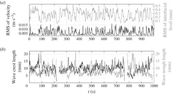
Figure 11 shows the average length of the wave crests and troughs for case 71 (b), along with the RMS of interfacial level and velocity (a). It is observed that the waves change from having crests longer than the troughs (characteristic of capillary waves), when the RMS of velocity is low (e.g. at
 $t\sim 50~\text{s}$
, 420 s), to having troughs longer than the crests (characteristic of gravity waves), when the RMS of velocity is high (e.g. at
 $t\sim 100$
s, 220 s, 780 s, 830 s). Although the time traces of the crest and trough lengths do not correspond exactly with the RMS traces due to the complexity of wave–turbulence interaction, they are nevertheless indicative of the process that occurs in the transitional region, i.e. when changing from the 2D SA to the 3D SA wave pattern.
5. Conclusions
In this study, experiments were performed in a horizontal pipe with stratified air/water flow, using PIV to measure the velocity fields and a profile capturing technique to measure the interfacial shapes. The gas and liquid flow rates were selected to cover the laminar–turbulent transition within the liquid layer in both the smooth (i.e. non-wavy) and the wavy region of the flowmap, as well as to cover the transition from the 2D small-amplitude to the 3D small-amplitude wave pattern.
Time traces of RMS values of the interfacial level and axial velocity (a) and wave crest and trough length (b) for case 71. At
 $t\sim 220~\text{s}$
and
 $t\sim 780~\text{s}$
, no wave quarters are detected, causing the lines in (b) to be discontinuous.

In the smooth region, the transition to turbulence occurred at increasingly smaller values of the Reynolds number
 $\mathit{Re}_{L}$
as the gas flow rate increased (figure 5). The range of
 $\mathit{Re}_{L}$
values where the first turbulent structures appeared was
 ${\sim}2500{-}2800$
, which corresponds to values typically measured in single-phase pipe flows (e.g. Wygnanski & Champagne Reference Wygnanski and Champagne1973; Schlichting Reference Schlichting1979). Furthermore, the results in figure 5 show that the transition occurs at (approximately) constant values of
 $u_{{\it\tau}}$
(and
 $u_{L}$
) for all gas flow rates. This indicates that, in the smooth region, the influence of increasing the air flow is to reduce the liquid height
 $h_{L}$
at which transition occurs, while the velocity stays essentially the same.
The Reynolds numbers in the wavy region were compared with those from the smooth region in relation to the laminar–turbulent transition (figure 6). The main conclusions are that (i) the introduction of waves does not influence the
 $\mathit{Re}_{L}$
at the beginning of transition (i.e. it continues to decrease in the expected way with increasing gas flow rate), but it increases the
 $\mathit{Re}_{L}$
where transition ends, and (ii) the transition in the wavy region occurs at increasing
 $u_{{\it\tau}}$
(and
 $u_{L}$
) with increasing gas flow rate.
The measured waves belonged to two wave patterns: 2D SA and 3D SA waves (e.g. Espedal Reference Espedal1998). The 2D SA wave pattern, with short (
 ${\sim}14~\text{mm}$
) waves of higher amplitude, was interpreted (using linear wave theory) as the capillary–gravity regime, and the 3D SA wave pattern, with long (
 ${\sim}22~\text{mm}$
) waves of lower amplitude, as the gravity–capillary regime. The measured wave celerity in all cases was very close to the minimum celerity predicted by the theory, and also the measured dependence between the wave celerity and the wavelength was correctly predicted by the theoretical dispersion relation (see figure 8
b). Furthermore, it appears that the transition from the 2D SA to the 3D SA wave pattern occurred through a period doubling (
 $2\rightarrow 1$
) bifurcation mechanism (as described by, e.g., Janssen (Reference Janssen1986), Bontozoglou & Hanratty (Reference Bontozoglou and Hanratty1990)), whereby the wavelength doubles from an initial value of 12.1 mm to 24.2 mm for air/water flow.
The time traces of the velocity and interfacial level presented in figures 10 and 11 showed that the development of intense turbulence tended to disrupt the waves. The waves occurring on such intense turbulent flow had a small wave height and troughs that were longer than the crests (a feature typical of gravity waves, see figure 11 b). This suggested that the change of the capillary–gravity regime to the gravity–capillary regime was a consequence of the development of turbulence in the liquid. On the other hand, the waves hindered the development of turbulence (§ 4.1.2). Based on this, it can be concluded that in the transitional region the two phenomena compete for dominance, both essentially suppressing the other. The explanation of this behaviour lies in the different nature of the two phenomena. The waves on a laminar mean flow are a coherent phenomenon, and this organised motion imposes a certain velocity profile, restricting the development of turbulence. On the other hand, as we have seen in figures 10 and 11, the developing turbulence tends to disrupt the wave structure. The waves in the turbulent region are, therefore, in a way a product of the underlying flow (which explains the irregularity of the gravity–capillary waves), while it is the opposite when the bulk flow is laminar.
Acknowledgement
The support of Shell Projects and Technology in financing this study is gratefully acknowledged.