Highlights
-
• We estimate an augmented Taylor rule based on a geopolitical risk (GPR) shock via constant and time-varying LP models.
-
• The panel evidence indicates that a geopolitical risk shock implies different monetary policy reactions in the short and medium run.
-
• In the short run, the central bank is more accommodative to limiting the negative effects on consumer sentiment.
-
• In the medium run, the central bank is more committed to combating inflation pressures.
1. Introduction
Escalation of these conflicts or a worsening in other geopolitical tensions could reduce economic activity and boost inflation worldwide, particularly in the event of prolonged disruptions to supply chains and interruptions in production. The global financial system could be affected by a pullback from risk-taking, declines in asset prices, and losses for exposed businesses and investors, including those in the U.S. — Financial Stability Report – October 2023.Footnote 1
After the global financial crisis, geopolitical considerations have increasingly influenced international trade relations. Indeed, it is now widely recognized that geopolitical risks and bilateral political tensions can have a strong influence on the functioning of the economy (Caldara and Iacoviello, Reference Caldara and Iacoviello2022). Geopolitical risk shocks affect the economy through different channels. Some of them are inflationary, such as the commodity price channel, especially the oil price (Mignon and Saadaoui, Reference Mignon and Saadaoui2024), and the currency channel (Gopinath, Reference Gopinath2015). In addition, other channels are deflationary, such as the consumer sentiment channel and the financial condition channel (Forbes and Warnock, Reference Forbes and Warnock2012). It is difficult to determine ex ante whether geopolitical risk shocks are inflationary or deflationary. Recent research suggests that geopolitical shocks tend to be inflationary throughout history (Caldara et al., Reference Caldara, Conlisk, Iacoviello and Penn2024).
In a more fragmented world, geopolitical risks may be a new and important factor that contributes to inflation pressures at the global level. The challenges raised by these new risks will become increasingly important to monetary policy and central bankers. These surges in geopolitical risks are also the by-product of changes in the global economy. During the past 20 years, the global economy has experienced several important changes. When it comes to global GDP, emerging countries, such as the BRICS country groupFootnote 2 now weigh more heavily than when China became a member of the WTO in December 2001. Therefore, the analysis of the reaction of monetary policy to geopolitical risks must be conducted at the global level instead of focusing exclusively on developed economies with highly developed financial markets and sound financial institutions. Consequently, considering a large sample of emerging and developed countries will be especially relevant to our research question.
Since the early 2000s, the world economy has faced numerous geopolitical events (e.g., 9/11, the first war in Ukraine, the China-U.S. trade dispute, the COVID-19 pandemic, and the second war in Ukraine), which underscore how geopolitical risks may impact an increasingly interconnected global economy. The integration of economies, facilitated by international trade, finance, and technology, can amplify the effects of these global events. Several authors found convincing evidence of a global business cycle (e.g., Kose et al. Reference Kose, Otrok and Whiteman2003, Monfort et al. Reference Monfort, Vitale and Renne2003, Ciccarelli and Mojon, Reference Ciccarelli and Mojon2010, Ginn, Reference Ginn2023 a, Ginn, Reference Ginn2023 b). Moreover, Miranda-Agrippino and Rey (Reference Miranda-Agrippino and Rey2020) have demonstrated the existence of a global financial cycle, where the dollar and US monetary policy play a pivotal role, especially after the Global Financial Crisis (GFC). The existence of the global business cycle and the global financial cycle implies that economic and financial conditions are not isolated events within individual countries, but are part of a larger global phenomenon. Policymakers can respond to global shocks by implementing accommodating monetary policies to counteract negative impacts on economic activity and limiting international financial spillovers.
High levels of uncertainty can affect the economic decision-making of individuals and companies, based on the theory of real options (Bernanke, Reference Bernanke1983), where uncertainty can increase the option value of waiting (Bloom, Reference Bloom2009). Empirical evidence suggests that when economic uncertainty is high, it can suppress investment for firms (e.g. Kang et al. Reference Kang, Lee and Ratti2014, Handley and Limao, Reference Handley and Limao2015), equity returns (e.g. Antonakakis et al. Reference Antonakakis, Chatziantoniou and Filis2013, Kang and Ratti, Reference Kang and Ratti2013, Arouri et al. Reference Arouri, Estay, Rault and Roubaud2016, Ginn, Reference Ginn2023 a); employment (e.g., Caggiano et al. Reference Caggiano, Castelnuovo and Groshenny2014, Caggiano et al. Reference Caggiano, Castelnuovo and Figueres2017); and production (Baker et al. Reference Baker, Bloom and Davis2016). Azzimonti and Talbert (Reference Azzimonti and Talbert2014) find that emerging market economies are more polarized and exhibit greater uncertainty, leading to polarized business cycles. Our empirical investigation will focus on the effects of geopolitical risks as an exogenous source of uncertainty. In this sense and more directly related to our study, Eckstein and Tsiddon (Reference Eckstein and Tsiddon2004) find that wars and periods of terrorism reduce the value of the “future” relative to the “present” resulting in lower output and welfare. Consequently, geopolitical uncertainty leads to a “wait-and-see” approach, thereby influencing the decision of economic agents. This could be illustrated by the consumer sentiment channel explored in Caldara et al., Reference Caldara, Conlisk, Iacoviello and Penn2024).
This cautious behavior may be more elevated during states of high geopolitical risk, further exacerbating economic downturns (Benchimol, Reference Benchimol2016). Elevated geopolitical risks can, in turn, raise the stakes for policy makers who are faced with ways of maintaining macroeconomic stability. Alan Greenspan, the US Federal Reserve Chair from 1987 to 2006, stated that “uncertainty is not just a pervasive feature of the monetary policy landscape; it is the defining characteristic of that landscape.”Footnote 3 The effect of geopolitical risks is not confined to individual countries and can therefore spill over to other countries and regions of the world economy. Domestic financial conditions can become vulnerable to global shocks, which can complicate monetary policy decisions (Kamin, Reference Kamin2010). Increased interconnectivity can make countries more susceptible to financial contagion that can originate domestically or abroad and jeopardize economic stability. Although comovement in domestic inflation rates may be related to cyclical fluctuations in the world economy, as shown by Woodford (Reference Woodford2007), globalization does not affect central banks’ ability to control domestic inflation through national monetary policy.
The US Federal Reserve Chair, Jerome Powell, identifies GPR as a major challenge of monetary policy (Powell, Reference Powell2019). Carney (Reference Carney2016) posits that there are three components, namely geopolitical risk, economic uncertainty, and policy uncertainty, established as an “uncertainty trinity,” which could adversely affect economic conditions. Since 2017, the European Central Bank and the International Monetary FundFootnote 4 have identified geopolitical tensions and geoeconomic fragmentation as a major risk to macroeconomic and financial stability. Understanding how monetary policy is influenced by geopolitical conditions is of paramount interest, both from the perspective of policy makers and from the perspective of the public.
This paper provides two novelties to the literature. First, we examine the macroeconomic effects of a geopolitical risk shock on policy reaction through a balanced panel LP model based on a rich data set of 18 economies that represent more than 75% of the global output.Footnote 5 Second, this is the first paper to test the hypothesis that the effect of a geopolitical risk shock on monetary policy is time-varying, with the expectation that its effects are likely to differ depending on different time horizons. In the short term, the central bank may seek to limit the negative effects on consumer sentiment by reducing the interest rate. In the medium term, the central bank is more eager to fight inflation pressures.
Consequently, periods marked by high geopolitical risk have potentially adverse consequences for an economy. Central banks, when implementing monetary policy, consider the prevailing economic conditions, including the geopolitical context. The Taylor rule provides a framework for central banks to adjust interest rates based on economic indicators, and this adjustment can be influenced by the level of the GPR (Taylor, Reference Taylor1993). First, the panel LP indicates that a geopolitical risk shock corresponds to a more accommodative monetary policy to limit the negative effects on consumer sentiment; second, the panel LP indicates that the monetary policy reaction is different in the medium run, as the central bank is more keen to fight inflation pressure; third, time-varying local projection (TVP-LP) estimates confirm these patterns for the Bank of England, the Bank of Canada, and the Bank of Israel. The timing of the shock (after the GFC), the size of the shocks, and the energy price context (elevated oil prices) appear to be important factors shaping these time-varying effects. The remainder of this paper is structured as follows. Section 2 describes the data. Section 3 discusses the empirical results. Section 4 concludes.
2. Data
To consider the global impact of geopolitical risk, we use a rich data set of industrial production, consumer price index (CPI), short-term interest rate, and GPR for 18 economies that represent more than 75% of global GDP to analyze the effect of GPR on interest rates. These 18 economies include: Switzerland (CHE), Chile (CHL), Canada (CAN), China (CHN), Columbia (COL), Czech Republic (CZE), the Euro zone (19 countries; EUR), the United Kingdom (GBR), Hungary (HUN), Ireland (IRL), India (IND), Israel (ISR), Japan (JPN), Mexico (MEX), South Korea (KOR), Poland (POL), Sweden (SWE), and the United States (USA). We used monthly data that covers the period from February 2000 to February 2022.Footnote 6 The growth variables are defined as year-on-year. The data are summarized in Table 1. All variables are converted to logarithm and, where appropriate, seasonally adjusted using the ARIMA X-12 algorithm of the US Census Bureau, except for the interest rate.
The GPR data for these 18 economies are taken from Matteo Iacoviello’s website.Footnote 7 Although the GPR data do not include a measure for the Euro area, we construct a Euro area GPR index based on sampled economies within the Euro area using a nominal GDP weighted index. The euro area GPR indicator includes the GPR indices of Belgium, Finland, France, Germany, Italy, the Netherlands, Portugal, and Spain. The weight of each economy in the index is derived from its economic size (proxied using quarterly nominal GDP data). We then apply the weights to each of the respective global indicators in the respective month, considering that the data are monthly. We plot the individual economies of the euro area and the constructed euro GPR index in Figure 1.
Variable selection

Euro area GPR indexes.

The international data for the explained and explanatory variables of the 20 economies are shown in Figure 2. In the output growth data, we can clearly see three episodes of global slowdown, namely the Internet Bubble in 2001, the Global Financial Crisis in 2008-2009, and the pandemic in 2020. The graphs for inflation show a more dispersed situation over time and between countries, except for the Global Financial Crisis and after the pandemic. In terms of monetary tightening and loosening, we also observe that the monetary cycles induced by the Global Financial Crisis (loosening) and after the pandemic (tightening) are the most synchronized episodes. During the most recent period, we can observe elevated levels of GPR due to the War in Ukraine. More generally, the GPR has seen large spikes around 2001 due to 9/11 and after 2009 due to rising tensions between the United States and China and the election of Donald Trump, as discussed in Mignon and Saadaoui (Reference Mignon and Saadaoui2024).
3. Empirical specification
The Taylor rule is designed to capture the reaction of central banks to deviations in inflation and output (Taylor, Reference Taylor1993). By examining the augmented rule, this research may offer insight into how central banks adjust interest rates in response to GPR shocks. The LP model, developed by Jordà (Reference Jordà2005), is used to estimate an augmented Taylor rule based on a GPR shock. Periods marked by high GPR have potentially adverse consequences for an economy. Central banks, when implementing monetary policy, consider the prevailing economic conditions, including states of geopolitical risks. The Taylor rule provides a framework for central banks to adjust interest rates based on economic indicators. We use this framework to test whether this adjustment can be influenced by the level of the GPR.
International economic data.

3.1 Baseline model
We start our empirical investigations with a Taylor rule augmented with geopolitical risks.Footnote 8 Following Aizenman et al. (Reference Aizenman, Hutchison and Noy2011), we use a lagged term for the short-term interest rate to consider inertia in the decisions of the monetary authorities. In order to establish some static evidence on the effects of GPR, we also include lags for the GPR term. These lags are set to 12 months to consider the horizon of monetary policy cycles. In addition, we include a dummy variable to control the impact of recession periods. We exclude BRA, and RUS from the panel of emerging countries as graphical evidence designating them as outliers and for data quality reasons. We estimate the following model for 18 economies (nine developed economies and nine emerging economies) from February 2000 to February 2022:
 \begin{equation} R_{i,t} = \alpha _0 + \alpha _i + \beta _{1} R_{i,t-12}+\beta _{2} {\textit {GAP}}_{i,t-1} + \beta _{3} \textit {{INF}}_{i,t-1} + \beta _{3} {\textit {GPR}}_{i,t-12} + \beta _{4} {\textit {REC}}_{i,t-1} + \epsilon _{i,t} \end{equation}
where
 $\alpha _0$
is a constant term,
 $\alpha _i$
are country fixed effects to control for unobserved cross-country heterogeneity,
 $R$
, stands for the short-term interest rate;
 $\textit {GAP}$
, the centered moving average of the output gap;
 $\textit {INF}$
, is the year-on-year inflation rate;
 $\textit {GPR}$
, stands for the GPR index, and
 $\textit {REC}$
, is the recession dummy.
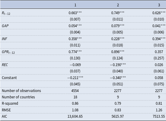
In Table 2, we can see that the Taylor rule has the expected signs.Footnote 9 The lag for the short-term rate is positive, which means that there is inertia in monetary policy decisions. This inertia is somewhat higher in developed countries. The policy reaction to positive output gaps is stronger in developed countries. In addition, the reaction to inflation is stronger in emerging countries. More interestingly, the impact of the GPR lag is positive and significant. A unit shock on the GPR variable results in an increase of a 0.9 percentage point on short-term interest rates twelve months later. As underlined by Iacoviello (Reference Iacoviello2024), geopolitical risk can adversely affect inflation. First, supply and trade disruptions can affect commodity prices (like the oil price, the price of rare earth elements, for example) and, in turn, increase inflation. Second, monetary and fiscal policy responses may, in turn, increase inflation if aggregate demand is excessively stimulated. Third, adverse effects on (consumer) confidence and aggregate demand can decrease inflation.Footnote 10 In our panel data, we can see that the total effect is driven by developed countries that aim to temper inflation following GPR shocks. After having established this first empirical evidence, we will examine the dynamic effect in the following. One may conjecture that the adverse effects of the GPR shock on confidence will be more impactful in the short run. In addition, the impact of supply disruption and the policy response will materialize in the medium term.
Panel Taylor rule augmented with geopolitical risks

Note: The dependent variable is the short-term interest rate. Model 1 is the model for the full sample. Model 2 is the model for the developed countries sample. Model 3 is the model for the sample of emerging countries. The symbol *** indicates statistical significance at the one percent level.
3.2 Panel local projections
In the linear specification, we estimate the nominal interest rate for the country
 $i$
at the time
 $t$
as follows:
 \begin{equation} R_{i,t+h} = \alpha _0 + \alpha _i +\beta _{h} S_{i,t-k} + \sum _{j=1}^{k} \nu ^\prime _j \mathbf {X}_{i,t-j} + \epsilon _{i,t+h} \end{equation}
where
 $\alpha _0$
is a constant term,
 $\alpha _i$
are country fixed effects to control for unobserved cross-country heterogeneity, and
 $S_{i,t}$
is a one unit shock to GPR. The vector
 $\mathbf {X}_{i,t}$
of control variables is the same as in Equation (1). Following Jordà and Taylor (2024), we proceed to a lag-augmentation to consider non-stationarity. Besides, lag-augmented Local Projections (LP) perform similarly to the Newey-West correction. We add one lag for the shock and control variables (thus,
 $k=2$
).
 $\epsilon _{i,t}$
relates to the error term. The coefficient
 $\beta _h$
in Equation (2) traces the effect of a GPR shock at the time
 $t$
on the policy reaction at the time
 $t+h$
. Impulse response functions (IRF) are presented in Figure 3 using 90% and 95% confidence bands. Consequently, the IRFs suggest that a GPR shock implies a higher interest rate for horizons superior to twelve months. This in line with the insights of Iacoviello (Reference Iacoviello2024) that suggest that GPR shocks produce higher inflation in the medium run using historical data, which are by empirical evidence (Caldara et al., Reference Caldara, Conlisk, Iacoviello and Penn2024).Footnote
11
GPR on interest rates (Full sample).
Note: shock is a unit shock to GPR. SE are bootstrapped (200 replications) and clusterized at the country level. Source: authors’ calculations.

At the 12-month horizon, the interest rate increased by 0.5 percentage points following a unit shock of geopolitical risks. In the following, we can also check whether this effect is driven by developed countries, such as in the panel FE exercises in Table 2. The results are in line with the baseline results, and the reaction to GPR is driven by developed countries, as can be seen in Figure 4. In the case of emerging economies in Figure 5, it is interesting to see that the impulse response function has a similar value around 0.5 percentage points at the 12 month-horizon.
GPR on interest rates (Developed countries).
Note: the shock is a unit shock to GPR. SE are bootstrapped (200 replications) and clusterized at the country level. Source: authors’ calculations.

GPR on interest rates (Emerging countries).
Note: the shock is a unit shock to GPR. SE are bootstrapped (200 replications) and clusterized at the country level. Source: authors’ calculations.

3.3 Time-series local projections
We also run individual local projection estimates to determine the medium-term effects of geopolitical risk on monetary policy. For each, we have 265 monthly observations from February 2000 to February 2022. The specification will be similar to the one in the previous section adapted to the time-series context. First, we can confirm that the group of developed countries shows more similar impulse responses compared to the group of emerging countries. In the developed-country group, the effect of GPR shocks produces an increase in the short-term interest rate 12 months later, confirming our baseline results in Figure 3 with different levels of significance. In the emerging-country group, we have more heterogeneous reactions to geopolitical risks. The impulse response functions are less smooth than in the case of developed countries.
GPR on interest rates (United Kingdom).
Note: the shock is a unit shock to GPR. LP stands for local projections, GPR for the GPR index, and RATE for the short-term interest rate. IRF coefficients for exogenous variables are dynamic multipliers. Source: authors’ calculations.

In the following, we focus on the most reactive central banks to GPR shocks.Footnote 12 We start with the United Kingdom in Figure 6. Likewise, we can note that the US and the euro area have similar impulse response functions at longer time horizons (see Appendix E). In the UK, the level of geopolitical risk fluctuates between .5 and 2 with spikes in September 2001 (9/11), March 2003 (Iraq War), and July 2005 (London bombings). Although short-term interest rates have been lower after the global financial crisis, interest rates exhibit some variations, reaching almost 1 percent before the easing monetary cycle started due to the COVID-19 pandemic. The dynamics multipliers indicate that the interest rate is positively impacted by the shock of geopolitical risks. The peak effect is higher than in the baseline, with a maximum increase of 1 percentage point at horizons greater than 12 months. This is an important result, which confirms our baseline.
GPR on interest rates (Canada).
Note: the shock is a unit shock to GPR. LP stands for local projections, GPR for the GPR index, and RATE for the short-term interest rate. IRF coefficients for exogenous variables are dynamic multipliers. Source: authors’ calculations.

Another interesting case study is Canada , as shown in Figure 7. The biggest spikes in geopolitical risk occurred in September 2001 (9/11) and March 2003 (Iraq War), as in the case of the United Kingdom. In addition, short-term rates reach 2 percent before the US easing monetary cycle started due to the COVID-19 pandemic in 2020. The profile of the impulse response function is similar to that in the UK case. In addition, it is also in line with the results that we find in the panel data for the 18 economies. Dynamic multipliers indicate that short-term interest rates increase 8 months after a unit shock of geopolitical risk. This increase is around 1 percentage point on the horizon of 12 months. This result is higher than the baseline value, which is around 0.5 percentage points at the 12-month horizon. As in the case of the entire sample, these results are significant at the 5 percent level after 9 months after the shock.
GPR on interest rates (Israel).
Note: the shock is a unit shock to GPR. LP stands for local projections, GPR for the GPR index, and RATE for the short-term interest rate. IRF coefficients for exogenous variables are dynamic multipliers. Source: authors’ calculations.

Emerging countries have experienced several geopolitical risk shocks during our sample period. We can focus on Israel , whose geopolitical risk index peaked in May 2002 (Operation Defensive Shield) and in July 2006 (Lebanon War). The short-term interest rate has risen to almost 4 percent after the GFC easing monetary cycle. By the beginning of 2015, the interest rate had gradually dropped to zero. As in the case of the emerging country group, the impulse response function is relatively less smooth than for the developed country group. Similarly to the results of the whole sample, the short-term interest rate increases 9 months after a geopolitical risk shock, as shown in Figure 8. As in the case of Canada, this increase is around 1 percentage point at the 12-month horizon. This result is higher than the baseline value, in Figure 4, and significant at the 5 percent level.
3.4 Time-varying local projections
After having established a baseline result for our panel data and inspecting the most significant country case with time series data, we will explore the possibility of time-varying effects for geopolitical risk shocks using time-varying local projections (TVP-LP), introduced by Inoue et al. (Reference Inoue, Rossi and Wang2024). More intuitively, the TVP-LP approach will estimate a path estimator for each time horizon.Footnote
13
For example, at horizon
 $15$
, we have
 $T = 265$
months (from February 2000 to February 2022) and the horizon is equal to
 $h = 15$
months. Thus, we have
 $T - h = 265 - 15 = 250$
impulse response functions in Figure 9. That means that this path estimator does not constrain the response to be the same for each time horizon, allowing for smooth and flexible time-variation. For example, GPR shocks that occur during episodes of high oil prices may have different effects than in normal conditions. The standard local projections cannot uncover these differences, and, similarly, the state-dependent local projections constrain the response to be the same in each state. With these different estimates for the impulse response at each time horizon, it is possible to construct an interval estimator to detect the presence of instabilities / time-varying effects in the impulse response at each time horizon. In fact, intuition suggests that the effect of different geopolitical risk episodes may differ after the GFC, as the monetary policy regime radically changed at the global level. In addition, we can conjecture that the reaction of monetary policy will be different depending on the size of the GPR shock. The central bank may be more accommodating in the wake of a large GPR shock to restore household confidence. This, in turn, might explain why the effect for short-run horizons differs from those in the medium run. Finally, the effect of geopolitical risk shock may be different during recessions. The TVP-LP model can be formulated as follows:
 \begin{align} & R_{t+h}=c_{t+h}+\beta _{h, t+h} S_t+\sum _{j=1}^{2} v_{j, t+h}^{\prime } \mathbf {X}_{t-j}+\epsilon _{t+h} \quad h=0,1, \ldots \\ & \textrm {IRF}(h)=\beta _{h, t+h} \nonumber \end{align}
where
 $\mathbf {X}=\left (R, \textit {INF}, \textit {GAP}, S\right )^{\prime }$
. The vector of control variables includes the lagged values of the following variables: the short-term interest rate, R; the inflation rate, INF; the output gap, GAP; and the shock on the geopolitical risk index (GPR), S. The parameter of interest is the time-varying impulse response
 $\beta _{h, t+h}$
following a shock S on the geopolitical risk index. For each month, we obtain a specific impulse response function.
3.4.1 United Kingdom
We start with the case of the United Kingdom. As we can see in Figure 9, the impulse response functions demonstrate some patterns that vary over time. Some impulse response functions reach -1 percentage point in the short run (3 month horizon), while some reach + 3 percentage points in the medium run (15 month horizon). The central bank may be more accommodating in the short run to stabilize consumer confidence and, thus, aggregate demand. However, the central bank may be more cautious with inflation pressures caused by supply constraints and the second-round effects of fiscal and monetary expansion on aggregate demand.
GPR on interest rates in an unstable environment (United Kingdom).
Note: the shock is a unit shock to GPR. RATE stands for the short-term interest rate, GPR, stands for the geopolitical risk index. The black curve is the standard LP’s IRF, and the green lines depict the time-varying IRF. For each time horizon, we have an IRF. The time horizon for the IRF is 15 months. Source: authors’ calculations.

GPR on interest rates after Global Financial Crisis (United Kingdom).
Note: the shock is a unit shock to GPR. RATE stands for the short-term interest rate, GPR, stands for the geopolitical risk index. The black curve is the standard LP’s IRF, and the green lines depict the time-varying IRF. For each time horizon, we have an IRF. The time horizon for the IRF is 15 months. Source: authors’ calculations.

GPR on interest rates for the top quartile of GPR (United Kingdom).
Note: the shock is a unit shock to GPR. RATE stands for the short-term interest rate, GPR, stands for the geopolitical risk index. The black curve is the standard LP’s IRF, and the green lines depict the time-varying IRF. For each time horizon, we have an IRF. The time horizon for the IRF is 15 months. Source: authors’ calculations.

In Figure 10, we can see that the central bank is more reactive in taming inflation after the GFC. All point estimates of the impulse response functions are above .5, ten months after the geopolitical risk shock. Does the size of the shock matter? In Figure 11, we plot the impulse response functions for large GPR shocks (i.e., we select the months when the GPR values are above the third quartile). It appears that the Bank of England is more accommodating in the face of large GPR shocks, as we can see in Figure 11. The contrast with smaller GPR shocks appears to be more important in the short term (1 to 3 months), where the impulse response functions are more negative. This instability explains why we do not see any effect in the short term for the linear LP for the UK in Figure 6.
We present the time-varying parameter plots at two different time horizons to capture the effect of geopolitical risk shocks in the short and medium run in Figures 12 and 13. These time-varying plots are designed to detect instabilities. If the confidence intervals do not include the constant parameter line, we can reject the null of non-time-varying impulse response functions. At the 2-month horizon, we can see that the GPR shocks that occurred during the 9/11 attacks prompted an aggressive reaction from the central bank, to limit the negative effects on consumers’ sentiment.
In Figure 12, the impulse response functions differ significantly, at the 95 percent level, from the rest of the sample period, where the reaction is more muted. At the 15-month horizon, the reaction of the short-term interest rate to GPR shocks was positive, to fight inflation pressures, as confirmed in Figure 9. We find that the reaction is significantly stronger just before the GFC recession. At that time, the oil price was especially high (140 USD per barrel in July 2008). For the remainder of the sample period, we do not detect instabilities in the effect of GPR shocks on short-term interest rates. The effect is positive and significant, as shown in Figure 13.
Time-varying parameter plot at horizon
 $t = 2$
(United Kingdom).
The time-varying parameter for the IRFs is observed at the month 2 in Figure 9. At the beginning of the sample, the effect of a shock differs significantly from the constant parameter LP at the 5 percent level. The black line corresponds to the unique IRF at the horizon
 $t = 1$
in Figure 9. The black line corresponds to the series of IRF at the horizon
 $t = 2$
in Figure 9. When the interval formed by the black dotted lines does not include the zero line, then the IRF is statistically significant at the 5 percent level, implying time-varying effects. Source: authors’ calculations.

Time-varying parameter plot at horizon
 $t = 15$
(United Kingdom).
The time-varying parameter for the IRFs is observed at the month 15 in Figure 9. At the beginning of the sample, the effect of a shock differs significantly from the constant parameter LP at the 5 percent level. The black line corresponds to the unique IRF at the horizon
 $t = 15$
in Figure 9. The black line corresponds to the series of IRF at the horizon
 $t = 2$
in Figure 9. When the interval formed by the black dotted lines does not include the zero line, then the IRF is statistically significant at the 5 percent level, implying time-varying effects. Source: authors’ calculations.

3.4.2 Canada
We can now explore the case of Canada. In Figure 14, we plot the time-varying impulse response for Canada. It appears that the reaction of short-term interest rates to geopolitical risk shocks follows time-varying patterns. In particular, it appears that the Bank of Canada may be more keen to reduce its interest rate in the short run, with a maximum reduction of around 3 percentage points following a unit shock on GPR. In addition, the reaction is different in the medium run. The short-term interest rate increases 15 months after the shock, with a maximum augmentation of almost 4 percentage points.
In Figure 15, we show that the reaction to geopolitical risk shocks is more restrictive after the GFC. In fact, we no longer find this large decrease in the interest rate in the months following the shock. However, these results are not as straightforward as in the case of the United Kingdom, where all impulse response functions are above the constant-parameter LP estimates during the 5 months following the shock, see Figure 11. Does the size of the GPR shock matter in the case of Canada? The answer to this question is given in Figure 16. The results are clear-cut. As in the case of the United Kingdom, they indicate that the central bank is more accommodating in the wake of large GPR shocks (i.e., we select the months when the GPR values are above the third quartile).
In Figures 17 and 18, we show the time-varying parameter plots for two different time horizons after the shock. For the one-month horizons, we find significant instability in the impulse response functions during 9/11, where the monetary policy reaction was very aggressive to the negative effects on consumer sentiment. The interest rate was lowered by around two percentage points, whereas the reaction of the Bank of Canada was muted during the rest of the sample. For the 15-month horizons, the monetary policy reaction was especially strong before the GFC. We detect significant instability in the impulse response functions during several months preceding the GFC, similarly to the case of the UK in Figures 12 and 13. The reaction is even stronger in the case of Bank of Canada (an increase around 4 percentage points), than in the case of Bank of England (around 3 percentage points).
Together with the cases of the United Kingdom and Canada, we establish that this pattern corresponds to the baseline result obtained for the developed countries in Figure 4. Consequently, we have further evidence that the central bank reaction differs depending on the time horizon in developed countries. Following a GPR shock, this general pattern indicates that the central banks in the developed countries seek to limit the negative effects on consumer sentiment for both households and firms in the vicinity of the shock. To do so, the interest rate is lower in the first month after the shock to stabilize aggregate demand. However, the central bank reaction differs in the medium run. The central bank may decide to increase the interest rate to tame inflation pressures in the medium term, especially in periods where the price of oil is elevated, as was the case before the GFC.
In general, these results are in line with the recent work of Caldara et al., Reference Caldara, Conlisk, Iacoviello and Penn2024) and the findings of Iacoviello (Reference Iacoviello2024). Our work underscores that the dynamic effects of the GPR shocks depend on the time horizon and vary over time. The timing of the shock (after the GFC), the size of the shocks, and the energy price context (elevated oil prices) appear to be important factors shaping these time-varying effects.
GPR on interest rates in an unstable environment (Canada).
Note: the shock is a unit shock to GPR. RATE stands for the short-term interest rate, gpr, stands for the geopolitical risk index. The black curve is the standard LP’s IRF, and the green lines depict the time-varying IRF. For each time horizon, we have an IRF. The time horizon for the IRF is 15 months. Source: authors’ calculations.

GPR on interest rates after Global Financial Crisis (Canada).
Note: the shock is a unit shock to GPR. RATE stands for the short-term interest rate, GPR, stands for the geopolitical risk index. The black curve is the standard LP’s IRF, and the green lines depict the time-varying IRF. For each time horizon, we have an IRF. The time horizon for the IRF is 15 months. Source: authors’ calculations.

GPR on interest rates for the top quartile of GPR (Canada).
Note: the shock is a unit shock to GPR. RATE stands for the short-term interest rate, GPR, stands for the geopolitical risk index. The black curve is the standard LP’s IRF, and the green lines depict the time-varying IRF. For each time horizon, we have an IRF. The time horizon for the IRF is 15 months. Source: authors’ calculations.

Time-varying parameter plot at horizon
 $t = 1$
(Canada).
The time-varying parameter for the IRFs is observed at the month 1 in Figure 14. At the beginning of the sample, the effect of a shock differs significantly from the constant parameter LP at the 5 percent level. The black line corresponds to the unique IRF at the horizon
 $t = 1$
in Figure 14. The black line corresponds to the series of IRF at the horizon
 $t = 1$
in Figure 14. When the interval formed by the black dotted lines does not include the zero line, then the IRF is statistically significant at the 5 percent level, implying time-varying effects. Source: authors’ calculations.

Time-varying parameter plot at horizon
 $t = 15$
(Canada).
The time-varying parameter for the IRFs is observed at the month 15 in Figure 14. At the beginning of the sample, the effect of a shock differs significantly from the constant parameter LP at the 5 percent level. The black line corresponds to the unique IRF at the horizon
 $t = 15$
in Figure 14. The black line corresponds to the series of IRF at the horizon
 $t = 2$
in Figure 14. When the interval formed by the black dotted lines does not include the zero line, then the IRF is statistically significant at the 5 percent level, implying time-varying effects. Source: authors’ calculations.

GPR on interest rates in an unstable environment (Israel).
Note: the shock is a unit shock to GPR. RATE stands for the short-term interest rate, GPR, stands for the geopolitical risk index. The black curve is the standard LP’s IRF, and the green lines depict the time-varying IRF. For each time horizon, we have an IRF. The time horizon for the IRF is 15 months. Source: authors’ calculations.

GPR on interest rates after Global Financial Crisis (Israel).
Note: the shock is a unit shock to GPR. RATE stands for the short-term interest rate, GPR, stands for the geopolitical risk index. The black curve is the standard LP’s IRF, and the green lines depict the time-varying IRF. For each time horizon, we have an IRF. The time horizon for the IRF is 15 months. Source: authors’ calculations.

GPR on interest rates for the top quartile of GPR (Israel).
Note: the shock is a unit shock to GPR. RATE stands for the short-term interest rate, GPR, stands for the geopolitical risk index. The black curve is the standard LP’s IRF, and the green lines depict the time-varying IRF. For each time horizon, we have an IRF. The time horizon for the IRF is 15 months. Source: authors’ calculations.

Time-varying parameter plot at horizon
 $t = 2$
(Israel).
The time-varying parameter for the IRFs is observed at the month 2 in Figure 19. At the beginning of the sample, the effect of a shock differs from the constant parameter LP at the 5 percent level. The black line corresponds to the unique IRF at the horizon
 $t = 2$
in Figure 19. The black line corresponds to the series of IRF at the horizon
 $t = 2$
in Figure 19. When the interval formed by the black dotted lines does not include the zero line, then the IRF is statistically significant at the 5 percent level, implying time-varying effects. Source: authors’ calculations.

Time-varying parameter plot at horizon
 $t = 15$
(Israel).
The time-varying parameter for the IRFs is observed at the month 15 in Figure 9. At the beginning of the sample, the effect of a shock differs significantly from the constant parameter LP at the 5 percent level. The black line corresponds to the unique IRF at the horizon
 $t = 15$
in Figure 19. The black line corresponds to the series of IRF at the horizon
 $t = 15$
in Figure 19. When the interval formed by the black dotted lines does not include the zero line, then the IRF is statistically significant at the 5 percent level, implying time-varying effects. Source: authors’ calculations.

3.4.3 Israel
We can now explore the case of Israel. In Figure 19, we can see that the impulse response functions exhibit contrasted time-varying patterns, especially at longer time horizons. In particular, some impulse response functions record a very strong reaction of the Bank of Israel in terms of interest rate increase. In Figure 20, we show that these particularly strong reactions were observed before the GFC. After the GFC, the reaction was more similar to that of developed countries in the short run (two-month horizons), with a decrease in the interest rate of around -0.3 percent. We note some dispersion in the impulse responses in the medium run (15-month horizon). We are now asking the same question as we did regarding the United Kingdom and Canada: Does the size of the shock matter? We plot the answer in Figure 21. Unlike of the Bank of England and the Bank of Canada, the Bank of Israel has reacted very strongly to large GPR shocks (i.e., months in which the GPR values are above the third quartile). These differences may be explained by several characteristics that distinguish the Israeli economy from other developed countries. For example, the inflation rate was considerably higher before the GFC (above 4%). In addition, Israel was confronted with a higher level of geopolitical risk throughout the entire sample.
In Figures 22 and 23, we show the time-varying plots for the horizons of 2 and 15 months following a GPR shock. We find that the short-run reaction does not show any time-varying pattern. This is consistent with the very compact impulse response at shorter horizons in Figure 17. In addition, we detect significant instability for the medium-run response at the beginning of the sample. The monetary reaction to GPR shocks was particularly strong around the Operation Defensive Shield in March 2002 (an increase of around 5%).
4. Conclusion
This paper analyzes the effect of a GPR shock on the interest rate response constant parameter and time-varying LP models. The models are estimated based on a balanced panel of 18 economies observed between February 2000 and February 2022. This paper contributes to the literature on the conduct of monetary policy in two broad ways. The first is methodological, where our contribution introduces an augmented Taylor rule with GPR shocks. This augmented Taylor rule is estimated with panel LP models. This paper attempts to shed light on the impact of a GPR shock on monetary policy using panel LP models and time-varying LP models, controlling for endogenous relationships. The modeling framework in this paper further relaxes the assumption that the effect of a GPR shock is stable over time. The baseline model is extended to capture possible time-varying relationships in the data during periods of large GPR shocks, unconventional monetary policy, and economic recessions.
The second contribution is empirical. The panel LP model demonstrates that the reaction of monetary policy depends on the time horizon, especially in the developed country group. Following a GPR shock, the central bank is more accommodative to limit the negative effects on consumer sentiment. In the medium term, the central bank is more interested in limiting inflation pressures, which may be due to second-round effects. The time-varying local projections confirm these findings for the Bank of England, the Bank of Canada, and the Bank of Israel. At both short- and medium-term horizons, significant instabilities are detected in the impulse response functions before the GFC when the oil prices were high, and during large-scale geopolitical events, like 9/11 or the Operation Defensive Shield.
Overall, the empirical results confirm that the state of geopolitical conditions matters in relation to how GPR shocks influence the policy reaction. Our results strongly suggest that GPR shocks can influence how central banks apply the Taylor rule. In the short term, central banks may choose to be more accommodating in counteracting the negative effects of uncertainty on economic activity. Country Taylor rules reveal the presence of time-varying effects, especially for the United Kingdom, Canada, and Israel.
The findings of this area of research are of historical interest regarding policy implications. A starting point for short-term policy is to establish sources of vulnerability that could create economic risks. The findings of this paper serve to provide new information by analyzing the propagation mechanisms through which GPR shocks influence economic conditions as a source of vulnerability. Policymakers are increasingly vigilant about developments in the geopolitical arena.
Acknowledgements
The authors thank Robert Czudaj, Joscha Beckmann, Christoph Wegener, Katharina Priedl, Gilles Dufrénot, Menzie Chinn, Elena Pesavento, Jonathan Benchimol, Barbara Rossi, Yiru Wang, Julien Pinter, Kéa Baret, Laurent Clerc, and Vladimir Borgy, and all the participants of the 4th Workshop on Financial Econometrics and Empirical Modeling of Financial Markets: New Challenges for Monetary Policy and Financial Markets for invaluable guidance and helpful comments.
Appendix A. Robustness checks with time fixed effects
GPR on interest rates (Developed countries) with time fixed effects.
Note: the shock is a unit shock to GPR. SE are bootstrapped (200 replications) and clusterized at the country level. Source: authors’ calculations.

GPR on interest rates (Emerging countries) with time fixed effects.
Note: the shock is a unit shock to GPR. SE are bootstrapped (200 replications) and clusterized at the country level. Source: authors’ calculations.

GPR on interest rates (Full sample) with time fixed effects.
Note: the shock is a unit shock to GPR. SE are bootstrapped (200 replications) and clusterized at the country level. Source: authors’ calculations.

Appendix B. Target variable and shock
Interest rates and GPR. Source: authors’ calculations.

Appendix C. Extended lags specification
GPR on interest rates (Industrialized countries).
Note: the shock is a unit shock to GPR. SE are bootstrapped (200 replications) and clusterized at the country level. We augment the lags of the dependent variable, the shock, and the controls from 2 lags to 12 lags. Source: authors’ calculations.

Appendix D. State-dependent Local Projections à la Ramey and Zubairy (Reference Ramey and Zubairy2018)
GPR on interest rates (State-dependent LPs).
Note: the shock is a unit shock to GPR. LP stands for local projections, GPR for the GPR index, and RATE for the short-term interest rate. Source: authors’ calculations.

Appendix E. Impulse Response function (IRF) for the U.S. and the Euro Area
GPR on interest rates (United States).
Note: the shock is a unit shock to GPR. LP stands for local projections, GPR for the GPR index, and RATE for the short-term interest rate. IRF coefficients for exogenous variables are dynamic multipliers. Source: authors’ calculations.

GPR on interest rates (Euro area).
Note: the shock is a unit shock to GPR. LP stands for local projections, GPR for the GPR index, and RATE for the short-term interest rate. IRF coefficients for exogenous variables are dynamic multipliers. Source: authors’ calculations.