Two efficient localization algorithms for multilateration

Mauro Leonardi; Adolf Mathias; Gaspare Galati

doi:10.1017/S1759078709000245

Two efficient localization algorithms for multilateration

Published online by Cambridge University Press: 13 July 2009

Mauro Leonardi ,

Adolf Mathias and

Gaspare Galati

Show author details

Mauro Leonardi*: Affiliation:
Tor Vergata University, Via del Politecnico 1, 00131 Rome, Italy. Phone: +39 06 72597417; Fax: +39 06 72597532.
Adolf Mathias: Affiliation:
Deutsche Flugsicherung, Systemhaus, Am DFS-Campus 10, 63225 Langen, Germany. Phone: +49 6103 7074468; Fax: +49 6103 7072595
Gaspare Galati: Affiliation:
Tor Vergata University, Via del Politecnico 1, 00131 Rome, Italy. Phone: +39 06 72597417; Fax: +39 06 72597532.
*: Corresponding author: M. Leonardi Email: leonardi@disp.uniroma2.it

Article contents

Abstract
INTRODUCTION
THE PROPOSED MLAT ALGORITHMS
SIMULATION
CONCLUSION
References

Rights & Permissions

Abstract

Two localization algorithms for multilateration systems are derived and analyzed. Instead of the classical time difference of arrival (TDOA), a direct use of the time of arrival (TOA) is made. The algorithms work for arbitrary spatial dimensions and overdetermined systems. These derivations are tested in a real-case implementation with simulated data (in particular, the multilateration (MLAT) system installed on the Malpensa Airport in Milan was considered for the MLAT simulation and its possible extension to wide area multilateration (WAM) system was considered for WAM trials). The results are also compared with the present-day algorithms performance, mostly based on TDOA.

Keywords

MLAT WAM TDOA TOA

Information

Type: Original Article
Information: International Journal of Microwave and Wireless Technologies , Volume 1 , Special Issue 3: Surveillance systems for air and airport traffic control , June 2009 , pp. 223 - 229

DOI: https://doi.org/10.1017/S1759078709000245 [Opens in a new window]
Copyright: Copyright © Cambridge University Press and the European Microwave Association 2009

I. INTRODUCTION

Multilateration (MLAT) of mode S squitters/replies is an important location and identification system for surface traffic surveillance in large airports (such as, in Europe, Heatrow, Frankfurt, Fiumicino, etc). The system exploits the secondary surveillance radar (SSR) mode S and mode A/C signals in order to locate and identify transponder-equipped aircraft and vehicles without the need for additional, non-standard on-board facilities.

A typical MLAT system is made up of a number (e.g. 10–15) of measurement stations capable of receiving, time tagging, and transmitting to a central processing subsystem (CPS) the SSR replies (or, also, the spontaneously emitted replies, called squitters) emitted from the aircraft. The MLAT algorithms (running in real time in the CPS) locate aircraft and other vehicles usually using time difference of arrival (TDOA) concepts, i.e. a hyperbolic technique. Location is also possible for approach area surveillance, i.e. in the case of wide area multilateration (WAM).

Due to the evolution toward WAM, it is important to extend the MLAT coverage, with ad-hoc algorithms that also have high performance in case of targets far away from the airport.

Two localization algorithms for MLAT and WAM systems that operate on TOA measurements (instead of TDOA measurements) will be proposed in this paper. These algorithms do not have to resort to expensive hyperbola intersection algorithms; instead, they rely on a simple and efficient least-square method and on the solution of a single quadratic equation. A theoretical discussion between TOA and TDOA is given by Shin and Sung [Reference Shin and Sung1].

The proposed methods set themselves apart from the well-known efficient methods [Reference Schau and Robinson2–Reference Chan and Ho7] and use a derivation that is quite similar to the Bancroft's one used in global navigation satellite system (GNSS) applications [Reference Bancroft8]. These algorithms deliver simple formulas that easily generalize to arbitrary spatial dimensions as well as to over- and under-determined cases.

II. THE PROPOSED MLAT ALGORITHMS

We consider the situation where a target with unknown position p = (p ₁⋯p _d) ∈ ℝ^d emits an SSR reply at the unknown time instant t that is detected, after propagation through a medium with speed c, by a set K of receiving units. Each receiver k ∈ K is located at a well-known position p_k = (p _k,1…p _k,d) and receives the reply at the time instant t _k. Under the assumption that the time measurements are distributed with N(t _k, σ), the following probability density function results for the target position:

(1)

$f_x \lpar {\bf x}\rpar = \prod\limits_{k \in K} {1 \over {\sigma_r \sqrt{2\pi}}} e^{ -\, {\sigma_r^{-2} \over 2 } \ \lpar \vert {\bf x} - {\bf p}_{k}\vert - \vert {\bf x}_0 - {\bf p}_{k}\vert\rpar ^2} \eqno \lpar 1\rpar$

where x₀ is the real target position, and σ_r = cσ is the standard deviation of the range measurements ρ = ct _k (that is Gaussian distributed: N(ct _k, σ_r) by hypothesis).

For the whole set of squared distances between each receiving station and the target, it is possible to write a set of K equations:

(2)

$\eqalign{\vert {\bf p}_k - {\bf p}\vert^2 &= c^2 \lpar t_k - t\rpar ^2\comma \; \cr \vert {\bf p}_k\vert^2 + \vert {\bf p}\vert^2 - 2{\bf p}_k^T {\bf p} &= c^2 \lpar t_k - t\rpar ^2 \quad \hbox{ with } k = 1 \ldots K\comma \; \cr 2\lpar {\bf p}_k^T {\bf p} - c^2 t_k t\rpar &= \vert {\bf p}_k\vert^2 - c^2 t_k^2 + \vert {\bf p}\vert^2 - c^2 t^2\comma \; \cr} \eqno \lpar 2 \rpar$

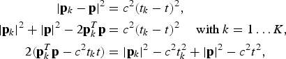
Defining the space–time vectors q = (p ₁…p _dt)^T, q_k = (p _k,1…p _k,dt _k)^T and the [K + 1, K + 1] matrix:

(3)

$S = \left(\matrix{1 &0 &0 &\cdots &0\cr 0 &1 &0 &\cdots &0\cr 0 &0 &1 &\cdots &0\cr \vdots &\vdots &\vdots &\ddots &\vdots \cr 0 &0 &0 &\cdots &-c^2\cr}\right)\comma \; \eqno \lpar 3\rpar$

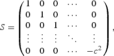
equation (2) can be arranged into the following equations system,

(4)

$2 \,Col \lpar {\bf q}_k^T\rpar S{\bf q} = Col \lpar {\bf q}_k^T S{\bf q}_k + {\bf q}^T S{\bf q}\rpar \eqno \lpar 4\rpar$

(where we make use of the Col(·) operator that stacks up its vector or matrix arguments x _k for all k in the index set K into a vector or matrix, respectively), and it is possible to introduce the scalar quantity v = q^TS q, obtaining

(5)

$2 \, Col \lpar {\bf q}_k^T\rpar S{\bf q} = Col \lpar {\bf q}_k^T S{\bf q}_k + v\rpar . \; \eqno \lpar 5\rpar$

Two direct approaches to solve this equation system in both the fully determined case, using the matrix inverse, and the overdetermined case, using the pseudo-inverse, can be used. Both cases will be denoted by the pseudo-inverse (the pseudo-inverse is a proper generalization of the inverse). Note that the pseudo-inverse provides a technique for linear least-square solutions in the face of additive white Gaussian noise that disturbs the time measurements t _k [Reference Kay9], and that we omit the notational burden of an error term in the equations below. Further note that, in reality, biases e.g. due to multipath propagation may be important cause of errors, which invalidates the assumption about the normally distributed error with zero mean.

A) Constant-v approach

System (5) can be solved for q (using the pseudo-inverse matrix (·)^† and forgetting hereafter that v depends on q):

(6)

$\eqalign{{\bf q} &= \textstyle{{1 \over 2}} \lpar Col \lpar {\bf q}_k^T\rpar S\rpar ^{\dagger} \cdot Col \lpar {\bf q}_k^T S{\bf q}_k + v\rpar \cr &= \underbrace{\textstyle{{1 \over 2}} \lpar Col \lpar {\bf q}_k^T\rpar S\rpar ^{\dagger} \cdot Col \lpar {\bf q}_k^T S{\bf q}_k\rpar }\limits_{\bf a} \cr &\quad + v \underbrace{\textstyle{{1 \over 2}} \lpar Col \lpar {\bf q}_k^T\rpar S\rpar ^{\dagger} \cdot Col 1}\limits_{\bf b} \cr} \eqno \lpar 6\rpar$

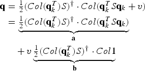
Introducing the vectors a and b that entirely depend on given values and expanding we obtain:

(7)

$v = {\bf a}^T S{\bf a} + v{\bf a}^T S{\bf b} + v{\bf b}^T S{\bf a} + v^2 {\bf b}^T S{\bf b} \eqno \lpar 7\rpar$

that becomes

(8)

$0 = {\bf a}^T S{\bf a} + v\lpar 2{\bf a}^T S{\bf b} - 1\rpar + v^2 {\bf b}^T S{\bf b} \eqno \lpar 8\rpar$

which is a quadratic equation for v with the solutions

(9)

$v_{1\comma 2} = {\lpar 1/2 \rpar - {\bf a}^T S{\bf b} \pm \sqrt{\lpar \lpar 1/2 \rpar - {\bf a}^T S{\bf b}\rpar ^2 - {\bf a}^T S{\bf a} {\bf b}^T S{\bf b}} \over {\bf b}^T S{\bf b}} \eqno \lpar 9\rpar$

Plugging either of these solutions into equation (6), the full solution for q, with the target position and emission time, is obtained. The solution can be found if the number of stations (measurements) K is larger than the spatial dimension d of the problem (e.g. four stations for three dimensional problem).

The choice of the appropriate value for v is the a challenging part of the algorithm and several ways can be followed:

– solution that leads to a positive target height can be chosen;
– the radicand (1/2 − a^TS b)² − a^TS ab^TS b may be negative due to the measurement noise; in this case only the real part of v can be taken into account.

In any case, all the real-world considerations should be taken into account when choosing the optimal solution.

REFERENCE SYSTEM SHIFT

A possible trick to simplify the problem can be the following one. If we introduce a reference system shift, choosing one station p_k as coordinate origin and its timestamp t _k as the time origin, we will have

(10)

$\eqalign{\vert {\bf p}_k - {\bf p}\vert^2 &= c^2 \lpar t_k - t\rpar ^2 \comma \cr \vert {\bf p}\vert^2 &= c^2 t^2 \comma \cr} \eqno \lpar 10\rpar$

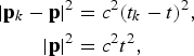
under the assumption that the reception time t _k is undisturbed. Consequently,

(11)

$v = {\bf q}^T S{\bf q} = {\bf p}^2 - c^2 t^2 = 0 \eqno \lpar 11\rpar$

and the problem of the choice of v vanishes.

Note that this is only a mathematical trick that works only under the assumption of no noise on the reception time t _k, this means that it will not necessarily produce better results.

B) Variable-v approach

The second way to solve equation (5) is shown in the following.

It is possible to introduce the vectors:

(12)

$\eqalign{{\bf r} &= \left(\matrix{{\bf p}\cr t\cr v\cr}\right) \comma \cr R &= Col \left({\bf p}_{k}^{T} - c^2 t_k - \textstyle{{1 \over 2}}\right)\comma \cr} \eqno \lpar 12\rpar$

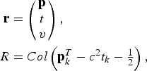
which allows us to arrange equation (5) as follows:

(13)

$\eqalign{2 \, Col \lpar {\bf q}_k^T\rpar S{\bf q} &= Col \lpar {\bf q}_k^T S{\bf q}_k + v\rpar \comma \cr 2 \, Col \left({\bf q}_k^T S{\bf q} - {v \over 2}\right)&= 2R{\bf r} = Col \lpar {\bf q}_k^T S{\bf q}_k\rpar \comma \cr} \eqno \lpar 13\rpar$

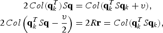
where we have used the property Col (q_k^T) S q = Col (q_k^TS q) and we have reminded ourselves that q_k^TS q = p_k^Tp − c ²t _kt.

Solving for r (in the minimum mean square error sense) we have

(14)

${\bf r} = \textstyle{{1 \over 2}} R^{\dagger} \, Col \lpar {\bf q}_k^T S{\bf q}_k\rpar . \eqno \lpar 14\rpar$

In this way the position of the target, the emission time of the reply, and v are calculated. The variable-v method does not take care of the relationship between p and v, but the v component of the solution r can be used to detect inconsistent solutions. In fact for |K| ≤ d + 2 and non-degenerate p_k, we obtain fully determined solutions for the variable-v approach, and

(15)

$\varepsilon = \vert {\bf p}\vert^2 - c^2 t^2 - v = \lpar {\bf p} - c^2 t - 1\rpar \cdot {\bf r} \eqno \lpar 15\rpar$

is the least-square approximation error. When it is zero (or near to zero considering the measurement noise), the solution can be considered consistent (which does not necessarily mean that it is correct). The quantity ɛ may be used to quickly detect and reject false individual time measurement (integrity monitoring or multipath monitoring) using the coding theory (see [Reference Mathias, Leonardi and Galati10] for more details).

III. SIMULATION

The two algorithms (i.e. constant and variable v) are tested for both MLAT and WAM Malpensa airport scenarios.

A) MLAT scenario

For the simulated scenario that reproduces the Malpensa airport situation as it is in 2008, where 10 receiver stations are installed on the airport surface, the receiver positions are shown in Table 1. All the quantities are expressed in meters, the height is expressed above the ground level (AGL) and the x-axis is parallel to the runway center line.

Table 1.

MLAT receiver station positions (in m).

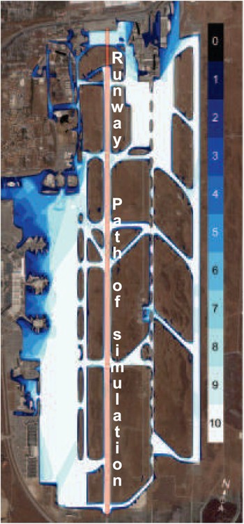
Not that all stations are visible from every point of the airport due to the blockage of line of sight by buildings. The visibility map (number of visible stations for each position on the airport) is shown in Fig. 1. This visibility information is taken into account to select which receiver stations must be used in the localization algorithms. All the simulations are referred to the runway center line displayed in Fig. 1. The measurement error (in m) for each station is imposed independent of the SNR (i.e. independent of the target–receiver distance) and equal to 0.3 m RMS. The error is calculated on 1000 simulation trials.

Fig. 1.

Number of visible stations from each point of the airport (the line shows the path used in the simulations).

The two algorithms proposed here are compared with the one well known in the literature, i.e. the Chan–Ho algorithm [Reference Chan and Ho7].

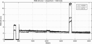
In Fig. 2 resulting RMS horizontal error for the simulated algorithms is plotted. The performance of the proposed methods is quite similar to the algorithms proposed in [Reference Chan and Ho7] but they are easier to implement and require less computational effort.

Fig. 2.

MLAT 2D position error. Only closed-form algorithms.

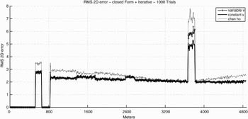
The importance of closed-form MLAT algorithms is their ability to produce an initial guess for an iterative position estimation process (using Taylor expansion around the guess, very accurate results are obtained if the guess is near the real position of the target). The MLAT position estimation capability with an iterative method is very much dependent on the initial guess and it is possible, using a wrong or too far guess, to have a divergence of the results. Therefore, here the usefulness of the proposed algorithms for initial guesses is compared to the other methods (Fig. 3).

Fig. 3.

MLAT 2D position error. Closed form + iterative algorithms.

A Taylor-based linearization of the localization problem with the initial guess as computed by own proposed (closed-form) algorithms is performed. In this case, for comparison, only the first approximation solution computed with the Chan–Ho algorithm is used (formula (14a) in [Reference Chan and Ho7]) as the precision solution is obtained by Taylor linearization in order to reduce the computational load for the CPS. Also for this context we have high performance in relation to the complexity of the algorithms: the location error for a target on an airport surface is, nearly everywhere, less than 4 m RMS (3 m using the iterative algorithms), i.e. well below the common 7.5 m requirements.

The error step between 3.6 and 3.8 km is due to the presence of the fire-brigade building between the two Malpensa runways that blocks the line of sight of the target from some stations, reducing the number of usable stations and increasing the geometric dilution of precision.

B) WAM Scenario

In the case of a wide area multilateration (WAM) scenario the typical condition changes are as follows: less stations, bigger measurement errors, and critical geometry. In this case a possible Malpensa Airport Wide Area Multilateration scenario was created and simulated.

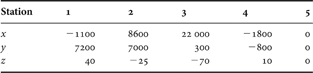
The possible receiver stations positions are reported in Table 2 as referred to the center of the airport. All the stations are imposed to be visible from the target position that run from 0 to 35 km ahead the runway (i.e. x axis) with a vertical angle of 3° simulating an aircraft landing. The measurement error for each station is imposed independent of the SNR and is equal to 0.5 m.

Table 2.

WAM RX simulated stations positions (m).

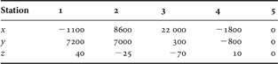
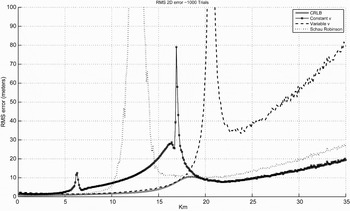
Figure 4 shows the 2D position error (RMS on 1000 trials) for the novel algorithms as compared with the Schau–Robinson [Reference Schau and Robinson2], commonly used in the case of target far from the receiver station and in a WAM scenario.

Fig. 4.

WAM 2D position error.

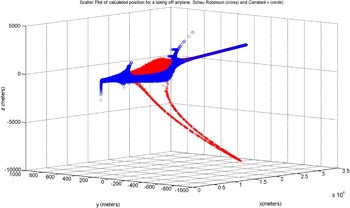
The peak error for the Schau–Robinson algorithms and the variable-v algorithm depends on the geometry that leads to the pseudo-inversion of an ill-conditioned matrix. In Fig. 5 the calculated position scatter plots for the constant-v (circle marker) and the Schau–Robinson (cross marker) algorithms on 50 simulation trials for each target position are also shown. The variable-v approach produces the best results for target positions near the airport but the performances are worse at long range. Results coming from the constant-v approach are much closer to the Cramer–Rao lower bound (CRLB, in particular, for targets far from the airport) and high error peaks are absent (for CRLB computation in case of MLAT please see [Reference Galati, Leonardi and Tosti11]).

Fig. 5.

Constant v (o) and Schau–Robinson (+) calculated position: scatter plot.

Moreover, the target position error is always below 10% of the airport distance. The error peak in the case of constant-v algorithms appears in proximity of a point in which the choice of solution for v change. This means that a proper rule to choose v is fundamental for this algorithm. It is also important to note that at about 22 000 m from the origin there is the last receiver station, after that the target is outside of the polygon that encloses the stations. This means that the constant-v algorithm works better for targets far from the receivers, while the variable-v algorithm works better for targets near the receivers.

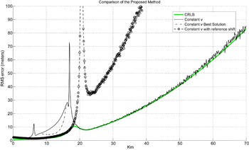
This can also be seen in Fig. 6 where a case study, in which the ‘ideal’ best solution between v ₁, v ₂ is always chosen (this is possible because in the simulation we know the real target position and we can choose the solution that produces the lower error), is reported. In this case study, we have maintained all the hypotheses of the previous case but we have extended the coverage area up to 70 km. The constant-v best solution line show the maximum performance for this method. The constant-v line shows the performance obtainable with the choosing rule as described in this paper (the positive one or the closest to the origin). Also the version is implemented here, this trick gives results identical to the variable-v. Finally, it is important to note that the performances of constant-v algorithms are very close to the CRLB.

Fig. 6.

Comparison between the constant v ‘ideal’ best solution, the constant v approach and the constant-v with reference shift.

IV. CONCLUSION

Two MLAT/WAM localization algorithms are designed and tested in a realist environment scenario simulation (Malpensa installation in Milan). The results show that these simple-to-implement and low-computational-load algorithms produce very competitive results, in particular if used as a first step to produce an initial guess for an iterative algorithm in case of MLAT scenario.

For the WAM scenario, the constant-v algorithm leads to promising performance that may also be improved by developing new decision rules for the v value, or implementing multiple hypothesis tracking algorithms. Another possible improvement can be the use of the constant-v algorithm for remote targets and variable-v algorithms for nearby targets.

Mauro Leonardi was born in 1974, in Rome. He obtained a Laurea cum laude in Electronic Engineering (May 2000) from Tor Vergata University in Rome and a PhD in October 2003, focusing his work on target tracking, air traffic control and navigation. From January 2004 he was Assistant Professor at Tor Vergata University in Rome, where he teaches ‘location and navigation systems’; ‘radar systems’ and ‘navigation satellite principles’. His main research activities are focused on: air traffic control and advanced surface movement guidance and control system (ASMGCS); satellite navigation, integrity and signal analysis.

Adolf Mathias graduated with diploma from the University of Karlsruhe, Germany in 1994. He was working in the field of art and media technology for over 10 years, his focus areas being virtual reality, panoramic visualization environments and advanced interactive scientific visualizations. He joined the German air traffic agency DFS in July 2005, where his main responsibilities are the research and implementation of algorithms for tracking and related areas.

Gaspare Galati Gaspare Galati was with the company Selenia from 1970 till 1986 where he was involved in radar systems analysis and design. From March 1986 he has been Associate Professor (and full professor from November, 1994) of Radar Theory and Techniques at the Tor Vergata University of Rome, where he also teaches probability, statistics and random processes. He is senior member of the IEEE, member of the IEE and of the AICT; within the AICT he is the chairman of the Remote Sensing, Navigation and Surveillance Group. He is the chairman of the SP and AES chapter of the IEEE. His main scientific interests are in radar, surveillance, navigation, and ATC/ASMGCS.

References

REFERENCES

[1]Shin, D.-H.; Sung, T.-K.: Comparisons of error characteristics between toa and tdoa positioning. IEEE Trans. Aerosp. Electron. Syst., 38 (2002), 307–311.CrossRef Google Scholar

[2]Schau, H.C.; Robinson, A.Z.: Passive source localization employing spherical surfaces from time-of-arrival differences. IEEE Trans. Acoust. Speech Signal Process., ASSP-35 (1987), 1223–1225.CrossRef Google Scholar

[3]Fang, B.T.: Simple solutions for hyperbolic and related position fixes. IEEE Trans. Aerosp. Electron. Syst., 26 (1990), 748–753.CrossRef Google Scholar

[4]Smith, J.O.; Abel, J.S.: Closed-form least-squares source location estimation from range–difference measurements. IEEE Trans. Acoust. Speech Signal Process., ASSP-35 (1987), 1661–1669.CrossRef Google Scholar

[5]Torrieri, D.J.: Statistical theory of passive location systems. IEEE Trans. Aerosp. Electron. Sys., AES-20 (1984), 183–198.CrossRef Google Scholar

[6]Urruela, A.; Riba, J.: Novel closed-form ml position estimator for hyperbolic location, in Proc. IEEE Int. Conf. Acoust, Speech and Signal Processing (ICASSP '04), Vol. 2, 17–21 May 2004, 149–52.Google Scholar

[7]Chan, Y.T.; Ho, K.C.: A simple and efficient estimator for hyperbolic location. IEEE Trans. Signal Process., 42 (1994), 1905–1915.CrossRef Google Scholar

[8]Bancroft, S.: An algebraic solution of the gps equations. IEEE Trans. Aerosp. Electron. Syst., Jan. 1985. 56–59.CrossRef Google Scholar

[9]Kay, S.M.: Fundamentals of Signal Processing–Estimation Theory, Prentice-Hall, Upper Saddle River. NJ, 1993.Google Scholar

[10]Mathias, A.; Leonardi, M.; Galati, G.: An efficient multilateration algorithm, in Proc. Tyrrhenian Int. Workshop on Digital Communications – Enhanced Surveillance of Aircraft and Vehicles TIWDC/ESAV 2008, 3–5 September 2008, 1–6.CrossRef Google Scholar

[11]Galati, G.; Leonardi, M.; Tosti, M.: Multilateration (local and wide area) as a distributed sensor system: Lower bounds of accuracy, in Proc. European Radar Conference EuRAD 2008, 30–31 October 2008, 196–199.Google Scholar