





1 Introduction
Cognitive diagnosis (CD) aims to provide detailed insights into students’ knowledge and skills, offering immediate feedback on their strengths and weaknesses in specific skills. However, most CD models (CDMs) were designed for binary responses and thus fall short in comprehensively analyzing incorrect responses. This limitation is particularly pronounced in the case of multiple-choice (MC) items because when binary CDMs are used to analyze CD data, conventionally, all distractors are collapsed into the incorrect answer, preventing the extraction of critical diagnostic information from the distractors of these MC items. To address this limitation, various CD methods designed specifically for MC items have been developed (e.g., de la Torre, Reference de la Torre2009; DiBello et al., Reference DiBello, Henson and Stout2015; Ozaki, Reference Ozaki2015; Wang et al., Reference Wang, Chiu and Köhn2023). Among them, the MC deterministic inputs, noisy “and” gate (MC-DINA) model (de la Torre, Reference de la Torre2009) stands out as the pioneer and has been extensively studied. The MC-DINA framework is characterized by a design that, in addition to the key, a subset of distractors—referred to as coded distractors—is also linked to certain q-vectors. These q-vectors carry additional diagnostic information and are systematically analyzed to enhance the classifications of examinees. A constraint imposed to the MC-DINA study was that the Q-matrix for each item had to follow the “stair-case” pattern: all the q-vectors assigned to the distractors had to be nested within that of the key, and each had to be nested within or nest the others. This constraint is unnecessarily stringent and, as a result, may result in immense difficulty on test development. In recent development on MC items, Wang et al. (Reference Wang, Chiu and Köhn2023) proposed to relax the stair-case structure of the q-vectors within an MC item with weaker assumptions. These regulations that guaranteed to produce proper and plausible items were later on formally stated and proved by Chiu et al. (Reference Chiu, Köhn and Wang2026).
Despite significant efforts to develop theoretically sound and practically accessible conditions for constructing feasible Q-matrices, some key statistical properties of the Q-matrix for MC items remain unexplored. One such critical property is completeness (Chiu et al., Reference Chiu, Douglas and Li2009; Köhn & Chiu, Reference Köhn and Chiu2017, Reference Köhn and Chiu2019, Reference Köhn and Chiu2021), which, when satisfied, ensures that all possible attribute profiles in the data can be identified. An incomplete Q-matrix may result in the misclassification of examinees into incorrect latent classes, leading to distorted interpretations of results and misguided pedagogical interventions. Hence, this property plays a crucial role in the development of diagnostic assessments and in making meaningful inferences about examinees’ skill mastery. Moreover, a complete Q-matrix is a fundamental assumption underlying several key theories in CD. Consequently, establishing conditions for Q-matrix completeness is of great importance. Without such conditions, these theories may lose their applicability or even become invalid because the validity of this essential assumption cannot be assessed. For example, Lin and Xu (Reference Lin and Xu2024) investigate the identifiability of model parameters for models with polytomous responses, specifically the GPDINA (Chen & de la Torre, Reference Chen and de la Torre2018) and sequential DINA models (Ma & de la Torre, Reference Ma and de la Torre2016). Both models belong to the class of DINA-type models. As in much of the identifiability literature for CDMs, their theorems rely on structural assumptions on the Q-matrix, among which Q-matrix completeness plays a fundamental role. However, Lin and Xu (Reference Lin and Xu2024) did not develop new conditions on Q-matrix completeness but relied on the sufficient and necessary Q-completeness lemma established in earlier work by Chiu et al. (Reference Chiu, Douglas and Li2009) because the GPDINA and sequential DINA models belong to the class of DINA-type models. The situation becomes more complicated when more general CDMs are considered. In the literature on identifiability for general CDMs—regardless of whether responses are binary or polytomous—the same completeness condition (i.e., requiring the Q-matrix to contain all single-attribute items) is typically adopted. However, while this condition is sufficient and necessary for the DINA/DINO model, it is only sufficient for other CDMs (see Proposition 1 in Köhn & Chiu, Reference Köhn and Chiu2017), including polytomous CDMs such as the model considered by Liu and Culpepper (Reference Liu and Culpepper2024). Consequently, existing identifiability results for these more general models may not characterize other Q-matrix structures that could also distinguish latent attribute patterns.
In light of these undesirable consequences, this study aims to establish sufficient and necessary conditions for determining the completeness of the Q-matrix for MC items. However, this problem is not a simple extension of the corresponding one for binary items. Because an MC item may contain additional diagnostic information through its coded distractors, directly forcing the key q-vectors of MC items to satisfy the sufficient and necessary conditions for a complete binary Q-matrix may be too restrictive. In the MC setting, such a construction may remain sufficient for completeness, but it is not generally necessary. The more fundamental question is therefore how the q-vectors associated with the key and coded distractors should be organized so that the resulting MC Q-matrix is complete. The present study addresses this question by establishing a theorem that provides sufficient and necessary conditions for the completeness of the Q-matrix for MC items. To support the proposed theorem, a lemma is developed, followed by corollaries that enhance its applicability. Note that all theoretical advancements are formulated under the proper and plausible conditions (Chiu et al., Reference Chiu, Köhn and Wang2026) and are rigorously justified through formal mathematical proofs.
The remainder of this article is organized as follows. First, the deterministic inputs, noisy “and” gate (DINA) model (Junker & Sijtsma, Reference Junker and Sijtsma2001), the associated conditions for Q-matrix completeness, existing CD methods for MC items, and the plausible and proper constraints for MC items are reviewed. Next, the proposed conditions for a complete Q-matrix for MC items are presented, along with practical guidance on how to construct a complete Q-matrix for MC items with minimal test length. A simulation study is then reported to illustrate the implications of the proposed theorem. Finally, the article concludes with a discussion of the main findings and limitations. Proofs of the lemma, theorem, and corollaries are provided in Appendix A.
2 Technical background
2.1 CD for dichotomized items
In CDMs, the cognitive skills assessed by an assessment are referred to as attributes. Assuming all attributes are binary and exhibit no hierarchical structure, if the assessment is used to measure K attributes,
$2^K$
 possible latent classes can be formed. Each latent class
$C_m$
 is defined by a K-dimensional attribute profile
$\boldsymbol {\alpha }_m = (\alpha _{m1}, \ldots , \alpha _{mK})^\prime $
 , where
$m=1,\ldots ,2^K$
 . Each entry
$\alpha _{mk}$
 in
$\boldsymbol {\alpha }_m$
 takes the value of 1 if the kth attribute has been mastered and 0 otherwise. For examinee i belonging to latent class
$C_m$
 , his/her attribute profile,
$\boldsymbol {\alpha }_i$
 , can also be denoted as
$\boldsymbol {\alpha }_m$
 .
For all CD analyses, the Q-matrix is an integral component, used to indicate relations between the test items and their required attributes. Suppose a test of J MC items measures at most K attributes. When the MC items are dichotomized to fit a binary CDM, only the q-vector of each key is specified and thus, the Q-matrix, denoted as
$\boldsymbol {Q}_{\text {B}}$
 , has the dimensions
$J \times K$
 . Similar to an examinee’s attribute profile
$\boldsymbol {\alpha }_i$
 , the q-vector of item j, denoted as
$\boldsymbol {q}_j$
 , is K-dimensional, with
$q_{jk} = 1$
 indicating that attribute k is required by item j and 0 otherwise.
2.1.1 The DINA model
The DINA model is the most extensively researched dichotomous CDM. Let
$\boldsymbol {Y}_i = (Y_{i1}, \ldots , Y_{iJ})^\prime $
 be the observed response vector of examinee i. The item response function (IRF) of the DINA model is defined as

where
$s_j$
 and
$g_j$
 represent the slipping and guessing parameters of item j, respectively, subject to the constraint
$0 < g_j < 1- s_j < 1$
 . The parameter
$\eta _{ij} =\prod _{k=1}^K\alpha _{ik}^{q_{jk}}$
 is the ideal response of examinee i to item j, indicating whether the examinee has mastered all the required attributes. Hence, the DINA model is a typical conjunctive model.
2.2 Completeness of
$\boldsymbol {Q}_{\text {B}}$
 for the DINA model

The concept of a “complete” Q-matrix was first discussed and proven in the asymptotic classification theory for CD (ACTCD; Chiu et al., Reference Chiu, Douglas and Li2009). A Q-matrix is said to be complete if it can identify all possible attribute profiles. Köhn and Chiu (2016) revisited the ACTCD and offered a more general definition of Q-matrix completeness based on the conditional expectation of the observed response given an examinee’s attribute profile. Formally stated, defining
$\boldsymbol {S}(\boldsymbol {\alpha })=E(\boldsymbol {Y}|\boldsymbol {\alpha })$
 , a test is complete if
$\boldsymbol {S}(\boldsymbol {\alpha })=\boldsymbol {S}(\boldsymbol {\alpha }^{\ast })$
 implies
$\boldsymbol {\alpha }=\boldsymbol {\alpha }^{\ast }$
 for all
$\boldsymbol {\alpha }$
 and
$\boldsymbol {\alpha }^{\ast }$
 . Based on the definition of completeness of the Q-matrix, Chiu et al. (Reference Chiu, Douglas and Li2009) and Köhn and Chiu (2016) established the sufficient and necessary conditions for a complete Q-matrix for the DINA model. The theorem states that
$\boldsymbol {Q}_{\text {B}}$
 is complete for the DINA model if and only if it includes all the
$\boldsymbol {e}_k$
 , where
$k = 1, \ldots , K$
 . Here,
$\boldsymbol {e}_k$
 denotes the
$1\times K$
 unit vector, with the kth entry being 1 and all other entries being 0. Detailed proof can be found in Chiu et al. (Reference Chiu, Douglas and Li2009) and Köhn and Chiu (2016).
2.3 CD for MC items
When traditional CDMs are used, the responses to all the distractors of an MC item are lumped together as the incorrect response. Consequently, the distractors remain unavailable for further analysis, resulting in the loss of valuable diagnostic information. A preferable approach is to employ CD methods specifically tailored for MC items, and the recent developments in CD for MC items are briefly presented below.
In the context of CD for MC items, not only the key but also all or a subset of the distractors are assigned specific q-vectors. In general, an option (which could be a key or a distractor) is said to be coded if it is assigned a q-vector. When the observed responses are analyzed using a CD method developed for MC items, the Q-matrix for MC items, denoted as
$\boldsymbol {Q}_{\text {MC}}$
 , is augmented from
$\boldsymbol {Q}_{\text {B}}$
 to account for the specification of q-vectors for the coded distractors. In this case, each MC item corresponds to a sub-Q-matrix,
$\boldsymbol {Q}_j$
 , with dimensions
$H_j^\ast\times K$
 , where
$H_j^\ast$
 is the number of coded options, expressed as follows:

where
$\boldsymbol {q}_j^{(H^\ast _j)}$
 is the q-vector of the key, and the others represent the q-vectors of the coded distractors.
$\boldsymbol {Q}_{\text {MC}}$
 is essentially the collection of all
$\boldsymbol {Q}_j$
 , having the dimensions (
$\sum _{j=1}^JH_j^\ast) \times K$
 . Based on this setup,
$\boldsymbol {Q}_{\text {MC}}$
 can be expressed as follows:

2.3.1 The MC-DINA model and its modifications
The MC-DINA model (de la Torre, Reference de la Torre2009), an extension of the DINA model, is the first CDM designed for MC items. In this study, a constraint that the q-vectors of the coded options were hierarchically nested was imposed, which limited the practicability of the model, and thus, all response options form ordinal options. Let
$\boldsymbol {X}_i = (X_{i1}, \ldots , X_{iJ})^\prime $
 be the observed response vector, and
$X_{ij}$
 can take on values
$h=1,\ldots ,H_j$
 , where
$H_j$
 is the number of options. Then, the ideal response of examinee i to MC item j is defined as follows:

where
$h^\prime $
 is recoded from h based on the number of skills required by the coded options. More required skills result in a larger
$h^\prime $
 , and noncoded options have
$h^\prime = 0$
 . Then, the IRF of the MC-DINA model is formulated as follows:

without further specifying how to find
$P_j(h \mid g)$
 .
The stringency of the nestedness constraint imposed on the MC-DINA model limits its applicability and was relaxed in the work by Wang et al. (Reference Wang, Chiu and Köhn2023). As a result, the coded options are no longer ordinal. To avoid ambiguity between notations, let l represent the level of responses without the nestedness constraint. Accordingly, the relaxed rule was proposed to level non-ordinal coded options: The key is assigned the highest level,
$H_j^\ast$
 , noncoded options are collapsed to the lowest level of 0, and each remaining coded distractor is assigned a unique value from
$\{1,\ldots ,H_j^\ast-1\}$
 based on two rules: the coded distractor with a longer length is assigned a higher value; if two coded distractors with the same length, the coded distractor with a higher lexicographic order is assigned a higher value. The ideal response to MC item j from examinee i,
$\eta _{ij}$
 , is then formulated as follows:

Equation (1) shows that the inclusion of this ideal response makes the MC-DINA model conjunctive, akin to the DINA model. The IRF of the MC-DINA model can then be explicitly written as follows:

subject to
$\sum _{c \neq l} \epsilon _{jcl}<0.5$
 for all items. In the above equation,
$\epsilon _{jcl}$
 is the probability that the observed response level c disagrees with the nonzero ideal response level l.
The MC nonparametric classification (MC-NPC) method (Wang et al., Reference Wang, Chiu and Köhn2023) is a nonparametric counterpart of the MC-DINA model that relaxes the nestedness constraint imposed in Reference de la Torrede la Torre’s (Reference de la Torre2009) MC-DINA model.
Its central idea is to classify examinees by comparing the observed response patterns with the ideal response patterns through a penalized Hamming distance, defined as

where
$w_j$
 is the penalty weight, formulated as

The attribute profile of examinee i is estimated by minimizing
$d_p(\boldsymbol {X}_i,\boldsymbol {\eta }^{(m)})$
 over all latent classes. Because the MC-NPC method does not require full parametric estimation of item parameters, it is computationally simpler and avoids some of the convergence difficulties that may arise in fitting the MC-DINA model. Wang et al. (Reference Wang, Chiu and Köhn2023) also reported that the MC-NPC model can provide more accurate classifications than the MC-DINA model in small-sample settings.
2.3.2 Plausible and proper conditions for
$\boldsymbol {Q}_{\text {MC}}$

It is important to note that removing the nestedness constraint described above does not imply that the coded options can randomly take any q-vectors. Köhn et al. (Reference Köhn, Chiu, Wang, Wiberg, Molenaar, González, Kim and Hwang2023) argued that the coded options of an MC item must be “proper” and “useful” to avoid ambiguity and redundancy, respectively. Chiu et al. (Reference Chiu, Köhn and Wang2026) further proposed two theorems to establish the conditions that can be used to determine whether MC items are proper and plausible (referred to as useful in the earlier work). Loosely speaking, item j is said to be plausible if and only if the q-vector of the key is not included within the q-vector of any coded distractor. This requirement prevents distractors from becoming redundant, because they must provide diagnostic information beyond the response options already available within the item. Furthermore, item j is proper if and only if either
$\boldsymbol {Q}_j$
 contains at most one coded distractor, or for each pair of the coded distractors, the union of their q-vectors must be included in
$\boldsymbol {Q}_j$
 , or the union must include
$\boldsymbol {q}_j^{(H_j^\ast)}$
 . This constraint helps avoid undesirable diagnostic ambiguity by ensuring that distractors are not equally likely to be chosen by an examinee.
3 Completeness of
$\boldsymbol {Q}_{\text {MC}}$
for the MC-DINA model

As discussed earlier, the completeness of a Q-matrix guarantees that all attribute patterns can be identified and thus is a statistical property that must be investigated before CD analysis can be properly and accurately performed. Completeness is also a key assumption of some important statistical properties, such as parameter identifiabilities (e.g., Gu & Xu, Reference Gu and Xu2018, Reference Gu and Xu2021; Lin & Xu, Reference Lin and Xu2024) and Q-optimality for CD-CAT (Xu et al., Reference Xu, Wang and Shang2016). The goal of this study is not to establish parameter identifiability for the MC-DINA model, but rather to establish the conditions for the completeness of a Q-matrix that allow practitioners to verify whether a given Q-matrix satisfies the completeness property when the data follow the MC-DINA model. Several important propositions implied by the theorem will also be discussed in this section.
3.1 Level-x design
Recall that when there are no hierarchical relations among the attributes,
$\boldsymbol {Q}_{\text {B}}$
 is complete if and only if it includes all the
$K\, \boldsymbol {e}_k$
 under the DINA model. It is therefore reasonable to presume that including all the
$\boldsymbol {e}_k$
 is essential for achieving the completeness of
$\boldsymbol {Q}_{\text {MC}}$
 . However, in the MC-DINA framework, a single MC item may include multiple
$\boldsymbol {e}_k$
 when some distractors are also coded. As a result, the major challenge here is to ensure that the assignment of the x distinct
$\boldsymbol {e}_k$
 , where
$1\leq x \leq K$
 , to the coded options within an MC item maximizes the effect of these
$\boldsymbol {e}_k$
 to distinguish
$2^x$
 attribute profiles. Specifically and importantly, these assignments cannot be random but governed by a) a particular arrangement such that every
$\boldsymbol {e}_k$
 can distinguish between examinees who have mastered attribute k and those who have not and b) by the plausible and proper rules. In this regard, new development on how to organize
$\boldsymbol {e}_k$
 in a
$\boldsymbol {Q}_{\text {MC}}$
 to guarantee the completeness are required.
Before the location of
$\boldsymbol {e}_k$
 can be identified, it is necessary to examine how examinees are classified with specific relations between coded distractors and the key. For notational convenience, the following partial-order notation is used: for two binary vectors
$\boldsymbol {a}$
 and
$\boldsymbol {b}$
 ,
$\boldsymbol {a} \succeq \boldsymbol {b}$
 denotes that
$a_k \geq b_k$
 for all k, and
$\boldsymbol {a} \succ \boldsymbol {b}$
 denotes that
$\boldsymbol {a} \succeq \boldsymbol {b}$
 and
$\boldsymbol {a} \neq \boldsymbol {b}$
 . Similarly,
$\boldsymbol {a} \preceq \boldsymbol {b}$
 and
$\boldsymbol {a} \prec \boldsymbol {b}$
 are defined analogously. Suppose item j contains a coded distractor, l. Given that the key is always selected when
$\boldsymbol {\alpha } \succeq \boldsymbol {q}_j^{(H_j^\ast)}$
 , the latent classes have three different types of ideal responses: l,
$H_j^\ast$
 , and
$l^\prime $
 , where
$l^\prime \neq l$
 ,
$l^\prime \neq H_j^\ast$
 , thereby classifying examinees into three corresponding groups, as shown in Table 1. Table 1 also demonstrates that based on whether
$\boldsymbol {\alpha } \succeq \boldsymbol {q}_j^{(H_j^\ast)}$
 , it is obvious that item j classifies examinees into two latent classes (i.e.,
$G_1 + G_2$
 vs.
$G_3$
 ). Further inspection reveals that examinees in
$G_1$
 have not mastered the attributes required by distractor l, and those in
$G_2$
 have mastered them. It is also true that if
$\boldsymbol {q}_j^{(l)} \prec \boldsymbol {q}_j^{(H_j^\ast)}$
 ,
$G_3$
 consists of examinees who have mastered attributes required by distractor l. However, if
$\boldsymbol {q}_j^{(l)} \not \prec \boldsymbol {q}_j^{(H_j^\ast)}$
 ,
$G_3$
 may be composed of examinees who have and have not mastered attributes required by distractor l. Hence, it is likely that item j will fail to identify all examinees who have mastered attributes required by distractor l.
Classes formulated by distractor l and the key of item j

Table 1 Long description
The table is structured with two main header rows and one main header column.
Top Header Row:
- The first two columns are grouped under the condition: bold alpha does not succeed bold q sub j super open parenthesis H sub j star close parenthesis.
- The third column is under the condition: bold alpha succeeds bold q sub j super open parenthesis H sub j star close parenthesis.
Second Header Row (Sub-conditions for the first group):
- Column 1: bold alpha does not succeed bold q sub j super open parenthesis l close parenthesis.
- Column 2: bold alpha succeeds bold q sub j super open parenthesis l close parenthesis.
Table Body:
- Row 1 (Ideal response):
- Column 1: l prime, where l prime does not equal l and l prime does not equal H sub j star.
- Column 2: l.
- Column 3: H sub j star.
- Row 2 (Class):
- Column 1: G sub 1.
- Column 2: G sub 2.
- Column 3: G sub 3.
When
$\boldsymbol {e}_{k}$
 is the focus, there are three possible scenarios for
$\boldsymbol {e}_k$
 : a)
$\boldsymbol {q}_j^{(H_j^\ast)} = \boldsymbol {e}_k$
 ; b)
$\boldsymbol {q}_j^{(l)} = \boldsymbol {e}_k$
 and
$\boldsymbol {q}_j^{(H_j^\ast)}\succ \boldsymbol {e}_k$
 ; and c)
$\boldsymbol {q}_j^{(l)} = \boldsymbol {e}_k$
 and
$\boldsymbol {e}_k \not \prec \boldsymbol {q}_j^{(H_j^\ast)}$
 . Based on the above discussion, item j in cases a) and b) can divide examinees into two groups: examinees who have and have not mastered attribute k. However, in case c), item j fails to do so. To demonstrate, take
$\boldsymbol {e}_{2}$
 as an example. Suppose there are four items designed to measure the mastery of attribute 2 (A2) when
$K=3$
 , and their Q-matrices and ideal responses of latent classes are shown in Table 2. Further assume that the four items do not contain other coded distractors than those listed in Table 2. In the table, the four latent classes that have mastered A2 are listed first, followed by the other four that have not mastered A2.
$\boldsymbol {Q}_1$
 and
$\boldsymbol {Q}_2$
 are used to demonstrate case a), where
$\boldsymbol {q}_j^{(H_j^\ast)} = \boldsymbol {e}_k$
 ;
$\boldsymbol {Q}_3$
 is used to exemplify case b), where
$\boldsymbol {q}_j^{(l)} = \boldsymbol {e}_k$
 and
$\boldsymbol {q}_j^{(H_j^\ast)}\succ \boldsymbol {e}_k$
 ; and
$\boldsymbol {Q}_4$
 shows case c), where
$\boldsymbol {q}_j^{(l)} = \boldsymbol {e}_k$
 and
$\boldsymbol {q}_j^{(H_j^\ast)} \not \succ \boldsymbol {e}_k$
 . Item 1 is equivalent to a binary item because it does not include any coded distractor. Therefore, latent classes who have mastered A2 can be differentiated from those who have not mastered. As for item 2 where
$\boldsymbol {q}_2^{(2)} = \boldsymbol {e}_2$
 and
$\boldsymbol {q}_2^{(1)} = \boldsymbol {e}_1$
 , latent classes who have mastered A2 were classified into
$G_3$
 with the ideal response of 2. Those who have not mastered A2 were classified into either
$G_2$
 or
$G_1$
 with the ideal response being either 1 or 0. Therefore, a
$\boldsymbol {Q}_j$
 satisfying
$\boldsymbol {q}_j^{(H_j^\ast)} = \boldsymbol {e}_2$
 can effectively differentiate between examinees who have mastered A2 and those who have not. In
$\boldsymbol {Q}_3$
 ,
$\boldsymbol {q}_3^{(2)}\succ \boldsymbol {e}_2$
 and
$\boldsymbol {q}_3^{(1)} = \boldsymbol {e}_2$
 . Consequently, examinees who have mastered A2 will select either the key or distractor, and those who have not mastered A2 will make a random selection among all options. Hence,
$\boldsymbol {Q}_3$
 can successfully distinguish between examinees who have mastered A2 and those who have not. With
$\boldsymbol {Q}_4$
 , examinees who have mastered both A1 and A2 (i.e.,
$(110)$
 and
$(111)$
 ) and those who have not mastered A2 but mastered A1 (i.e.,
$(100)$
 and
$(101)$
 ) are classified into
$G_3$
 . That is, mastery of A1, which is required by the key, masks the distinction between mastery and non-mastery of A2, even though
$\boldsymbol {e}_2$
 appears as a coded distractor. Therefore, item 4 is unable to differentiate between examinees who have mastered A2 and those who have not. In conclusion, if
$\boldsymbol {e}_k$
 is linked to a distractor but the key does not require attribute k, this item cannot fully distinguish between the mastery and non-mastery of attribute k.
Ideal responses to four items assessing the mastery of A2

Table 2 Long description
The table is organized into columns for four items: Q sub 1, Q sub 2, Q sub 3, and Q sub 4.
Header Information:
- Row 1: Q sub 1, Q sub 2, Q sub 3, Q sub 4.
- Row 2: q super (H sub j super asterisk) values are 010, 010, 110, and 100 respectively.
- Row 3: q super (l) values are dash, 100, 010, and 010 respectively.
Data Rows:
- Mastery of A 2 group:
- Profile (010): Q 1 = 1, Q 2 = 2, Q 3 = 1, Q 4 = 1.
- Profile (110): Q 1 = 1, Q 2 = 2, Q 3 = 2, Q 4 = 2.
- Profile (011): Q 1 = 1, Q 2 = 2, Q 3 = 1, Q 4 = 1.
- Profile (111): Q 1 = 1, Q 2 = 2, Q 3 = 2, Q 4 = 2.
- Non-mastery of A 2 group:
- Profile (000): Q 1 = 0, Q 2 = 0, Q 3 = 0, Q 4 = 0.
- Profile (100): Q 1 = 0, Q 2 = 1, Q 3 = 0, Q 4 = 2.
- Profile (001): Q 1 = 0, Q 2 = 0, Q 3 = 0, Q 4 = 0.
- Profile (101): Q 1 = 0, Q 2 = 1, Q 3 = 0, Q 4 = 2.
The above discussion and examples show that the inclusion of
$\boldsymbol {e}_k$
 alone is not sufficient to constitute a complete
$\boldsymbol {Q}_{\text {MC}}$
 ; the assignment of
$\boldsymbol {e}_k$
 is also crucial to its completeness. In particular, Table 2 illustrates that an item may contain
$\boldsymbol {e}_k$
 among its coded options but still fail to distinguish mastery from non-mastery of attribute k when the key masks this distinction. Hence, to establish the completeness of
$\boldsymbol {Q}_{\text {MC}}$
 , the level-x design is first developed and defined to properly organize
$\boldsymbol {e}_k$
 in
$\boldsymbol {Q}_{j}$
 .
The intuition underlying the level-x design is combinatorial. Because x binary attributes generate
$2^x$
 latent mastery patterns, an MC item intended to distinguish all mastery patterns generated by these x attributes must induce
$2^x$
 distinct ideal-response states. Since the all-zero mastery pattern corresponds to the noncoded option, at least
$2^x-1$
 coded options are required. However, this counting requirement alone is not sufficient: the corresponding q-vectors must also be arranged so that the item actually distinguishes the
$2^x$
 latent classes. This requirement motivates the following definition.
Definition 1. A
$\boldsymbol {Q}_j$
 is said to have a level-x design for
$x\geq 1$
 if x distinct
$\boldsymbol {e}_k$
 , where
$k = 1, 2, \ldots , K$
 , are linked to its coded options and it can distinguish
$2^x$
 latent classes constituted by these x attributes. If
$\boldsymbol {Q}_j$
 only contains one
$\boldsymbol {e}_k$
 but item j fails to distinguish between examinees who have mastered attribute k and those who have not,
$\boldsymbol {Q}_j$
 is said to have a level-0 design.
Two common designs in practice, the level-1 and level-2 designs, are discussed in detail below. Additionally, the level-3 design is briefly introduced as an illustration for understanding the level-x design. The section is wrapped up with a discussion of the level-0 design, a crucial case where the key masks the distinction established by
$\boldsymbol {e}_k$
 . Lemma 1 is then presented as a remedy for the level-0 design to differentiate examinees who have mastered attribute k from those who have not. Because the level-0 design is a case requiring special treatment, it is not included when referring to the level-x design in this study.
3.1.1 Level-1 design
Based on Definition 1, a
$\boldsymbol {Q}_j$
 is said to have a level-1 design if it can distinguish examinees who have mastered a particular attribute, say attribute k, from those who have not.
$\boldsymbol {Q}_1$
 and
$\boldsymbol {Q}_3$
 in Table 2 have level-1 designs. In contrast, although
$\boldsymbol {Q}_2$
 contains two
$\boldsymbol {e}_k$
 (i.e.,
$\boldsymbol {e}_2$
 and
$\boldsymbol {e}_1$
 ), it can only distinguish examinees who have mastered A2 from those who have not. Hence,
$\boldsymbol {Q}_2$
 also has a level-1 design. In conclusion, an MC item with a level-1 design can only determine the mastery of a single attribute and thus can be treated as an extension of a binary item under the DINA model, allowing for the utilization of an
$\boldsymbol {e}_k$
 to define either the key or a coded distractor. It is important to note that a
$\boldsymbol {Q}_j$
 with a level-1 design can include other coded distractors as long as the item stays useful and proper.
3.1.2 Level-2 design
A level-2 design allows a
$\boldsymbol {Q}_j$
 to identify the mastery of two attributes, say k and
$k^\prime $
 , where
$k\neq k^\prime $
 , so that
$\boldsymbol {Q}_j$
 can effectively distinguish examinees into four groups (i.e.,
$2^2=4$
 ): those who have mastered only attribute k, only attribute
$k^\prime $
 , both attributes k and
$k^\prime $
 , and neither attributes k nor
$k^\prime $
 . Notice that although
$\boldsymbol {Q}_2$
 and
$\boldsymbol {Q}_4$
 contain two distinct
$\boldsymbol {e}_{k}$
 , they do not have a level-2 design because they fail to identify examinees who have mastered both A1 and A2. The only way to achieve a level-2 design for these items is to define a coded option as
$\boldsymbol {e}_1+\boldsymbol {e}_{2}$
 subjective to
$\boldsymbol {e}_1+\boldsymbol {e}_{2} \preceq \boldsymbol {q}_j^{(H_j^\ast)}$
 . Consequently,
$\boldsymbol {Q}_j$
 must contain the following structure:

This means an item conforming to the level-2 design should include not only
$\boldsymbol {e}_k$
 and
$\boldsymbol {e}_{k^\prime }$
 but also
$\boldsymbol {e}_k+\boldsymbol {e}_{k^\prime }$
 . Note that an MC item whose Q-matrix has a level-2 design may include additional coded options as long as the item is proper and useful.
3.1.3 Level-3 design
Likewise, a
$\boldsymbol {Q}_j$
 with the level-3 design can differentiate among examinees who have mastered only one of the three attributes, namely, k,
$k^\prime $
 , or
$k^{\prime \prime }$
 , those who have mastered any two of them, all of them, and none of them, where
$k \neq k^{\prime } \neq k^{\prime \prime }$
 . After column swapping, a Q-matrix with a level-3 design has the following structure:

However, in practice, it is not common for an MC item to have seven or more coded options. Therefore, the level-3 design is not further discussed in the current article.
3.1.4 Level-0 design
As discussed above, a
$\boldsymbol {Q}_j$
 with the level-x design, for
$x\geq 1$
 , not only includes
$\boldsymbol {e}_k$
 but also distinguishes examinees who have mastered attribute k from those who have not. However, including an
$\boldsymbol {e}_k$
 does not necessarily guarantee the conformation of the level-1 design. A
$\boldsymbol {Q}_j$
 that contains an
$\boldsymbol {e}_k$
 but fails to make the distinction is said to have the level-0 design. Based on Definition 1, a
$\boldsymbol {Q}_j$
 has a level-0 design if distractor l is coded as
$\boldsymbol {e}_k$
 but
$\boldsymbol {q}_{j}^{(H_{j^*})} \not \succ \boldsymbol {e}_k$
 , as shown in the above case c).
$\boldsymbol {Q}_4$
 in Table 2, for example, is an item that has such a design. Therefore, to distinguish examinees who have mastered attribute k from those who have not, it is recommended to begin with a
$\boldsymbol {Q}_j$
 that contains
$\boldsymbol {e}_k$
 and has a level-x design. However, if such a
$\boldsymbol {Q}_j$
 is not available and
$\boldsymbol {e}_k$
 is included in items that only have a level-0 design, the immediate question is that whether it is possible to separate examinees who have and have not mastered attribute k apart by attaching more items to a level-0-design item. If the answer is yes, what is the procedure one should follow? Lemma 1 is developed to answer the above question. Before it is presented, an example, depicted in Figure 1, is used to illustrate and facilitate the reasoning.
An example set of items to distinguish between mastery and non-mastery of A2.

Figure 1 Long description
The flowchart begins at the top with a rectangular box containing (*, *, *). An arrow points down to a second box labeled Item 4: q sub 4 super (2) = (1, 0, 0), q sub 4 super (1) = (0, 1, 0). Three arrows branch from Item 4:
- Arrow G sub 2 points left to a diamond containing (0, 1, *).
- Arrow G sub 3 points down to a diamond containing (1, *, *).
- Arrow G sub 1 points right to a diamond containing (0, 0, *).
From the (1, *, *) diamond, an arrow points down to a third box labeled Item 5: q sub 5 super (2) = (1, 0, 1), q sub 5 super (1) = (1, 1, 0). Three arrows branch from Item 5:
- Arrow G sub 2 points left to a diamond containing (1, 1, 0).
- Arrow G sub 3 points down to a diamond containing (1, *, 1).
- Arrow G sub 1 points right to a diamond containing (1, 0, 0).
From the (1, *, 1) diamond, an arrow points down to a fourth box labeled Item 6: q sub 6 super (1) = (1, 1, 1). Two arrows branch from Item 6:
- Arrow G sub 3 points down to a diamond containing (1, 1, 1).
- Arrow G sub 1 points right to a diamond containing (1, 0, 1).
Revisit
$\boldsymbol {Q}_4$
 in Table 2. This item conforms to the level-0 design with the key and a coded distractor defined by
$\boldsymbol {q}_4^{(2)}=(1,0,0)$
 and
$\boldsymbol {q}_4^{(1)}=(0,1,0)$
 , respectively. After the item is administered, both
$(1,1,\ast)$
 and
$(1,0,\ast)$
 , where
$\ast$
 denotes an entry either 0 or 1, are assigned to
$G_3$
 because the item cannot separate them apart based on A2 (see Table 1). Notice that in this case, whether or not the next item requires A1 does not affect the differentiation between
$(1,1,\ast)$
 and
$(1,0,\ast)$
 because both have already mastered it. However, the requirement of A3 will mask the mastery of the A2 between
$(1, 1, 0)$
 and
$(1, 0, 0)$
 . Hence, to distinguish between
$(1, 1, \ast)$
 and
$(1, 0, \ast)$
 , an item with a coded option defined by
$(\ast,1,0)$
 is needed. If
$(\ast,1,0)$
 defines the key, then
$(1,1,\ast)$
 will be assigned to
$G_3$
 , and
$(1,0,\ast)$
 will be assigned to
$G_1$
 or
$G_2$
 . As a result, all the examinees can be separated apart based on A2. To illustrate a more complex scenario, assume that such an item is not available in the test.
Figure 1 illustrates how additional items are used to evaluate mastery of A2. The labels
$G_1$
 ,
$G_2$
 , and
$G_3$
 shown near the arrows denote the groups defined in Table 1. Item 5 with a coded distractor and the key defined by
$(1,1,0)$
 and
$(1,0,1)$
 , respectively, is presented to the examinees. After this item is administered,
$(1,1,1)$
 and
$(1,0,1)$
 are still mixed in
$G_3$
 and thus, more items are needed to separate them apart based on A2. Again, whether the next item requires A1 and A3 does not influence the differentiation between
$(1,1,1)$
 and
$(1,0,1)$
 . The requirement is that this item should consist of a coded option defined by
$(\ast,1,\ast)$
 . Item 6 has the key defined by
$(1,1,1)$
 and thereby can be used to distinguish
$\boldsymbol {\alpha }$
 from
$\boldsymbol {\alpha }^\ast$
 . Differing from the level-1 and level-2 designs, where only one item is needed to distinguish the examinees who have and have not mastered A2, in this example, two more items are required when the item containing
$\boldsymbol {e}_k$
 has a level-0 design.
The example above can be generalized as follows. Suppose item j contains
$\boldsymbol {e}_k$
 with a level-0 design used to distinguish the mastery of attribute k. After this item is administered, examinees are categorized into three classes, as shown in Table 1:
$G_1$
 (not mastered attribute k),
$G_2$
 (mastered attribute k), and
$G_3$
 (a mix of
$\boldsymbol {\alpha } \succeq \boldsymbol {e}_k + \boldsymbol {q}_j^{(H_j^\ast)}$
 and
$\boldsymbol {\alpha }^\ast \succeq \boldsymbol {q}_j^{(H_j^\ast)}$
 but
$\boldsymbol {\alpha }^\ast \not \succ \boldsymbol {e}_k$
 ). Here,
$G_3$
 consists of examinees who have and have not mastered attribute k and thus, additional items are required to distinguish between
$\boldsymbol {\alpha }$
 and
$\boldsymbol {\alpha }^\ast$
 in
$G_3$
 .
Let
$\boldsymbol {q} =\boldsymbol {q}_j^{(H_j^\ast)}$
 denote the attributes that examinees in
$G_3$
 have already mastered, which do not contribute to distinguishing between
$\boldsymbol {\alpha }$
 and
$\boldsymbol {\alpha }^\ast$
 . From the remaining items, select an item that has a coded option defined by
$\boldsymbol {e}_k+\boldsymbol {q}_0$
 , where
$\boldsymbol {q}_0 \preceq \boldsymbol {q}$
 . This item is required to differentiate
$\boldsymbol {\alpha }$
 from
$\boldsymbol {\alpha }^\ast$
 . Denote this item as
$j^{\prime }$
 . If
$\boldsymbol {q}_{j^{\prime }}^{(H_{j^{\prime }}^*)} \succ \boldsymbol {e}_k$
 , based on Table 1, this item can explicitly divide examinees in
$G_3$
 into two groups based on the mastery of attribute k. However, if
$\boldsymbol {q}_{j^{\prime }}^{(H_{j^{\prime }}^*)} \not \succeq \boldsymbol {e}_k$
 ,
$\boldsymbol {\alpha } \succeq \boldsymbol {e}_k + \boldsymbol {q}_0 + \boldsymbol {q}_{j^{\prime }}^{(H_{j^{\prime }}^*)}$
 and
$\boldsymbol {\alpha }^\ast \succeq \boldsymbol {q}_0 + \boldsymbol {q}_{j^{\prime }}^{(H_{j^{\prime }}^*)}$
 but
$\boldsymbol {\alpha }^\ast \not \succ \boldsymbol {e}_k$
 will be left in
$G_3$
 and remain un-separated. Update
$\boldsymbol {q} =\boldsymbol {q} \lor \boldsymbol {q}_{j^{\prime }}^{(H_{j^{\prime }}^*)}$
 . Thus, an item who has a coded option defined by
$\boldsymbol {e}_k+\boldsymbol {q}_0$
 , where
$\boldsymbol {q}_0 \preceq \boldsymbol {q}$
 , is required to distinguish
$\boldsymbol {\alpha }$
 from
$\boldsymbol {\alpha }^\ast$
 . The process continues with updating
$\boldsymbol {q}_0$
 and finding additional items until the mastery of attribute k is determined.
The process detailed above outlines the need for additional items to assess the mastery of attribute k when dealing with an item characterized by a level-0 design. Lemma 1, shown below, not only summarizes this process, but makes it more comprehensive, as item
$j^\prime $
 might not be unique in practice. The proof of Lemma 1 is presented in Appendix A.
Lemma 1. Suppose
$\boldsymbol {Q}_{j_0}$
 of item
$j_0$
 involving
$\boldsymbol {e}_k$
 conforms to the level-0 design; that is,
$\boldsymbol {q}_{j_0}^{(H_{j_0}^*)} \not \succ \boldsymbol {e}_k$
 . Consider the following algorithm:
-
Step 0. Let $\boldsymbol {q}=\boldsymbol {q}_{j_0}^{(H_{j_0}^*)}$
and initialize set
$\mathcal {J}=\{j_0\}$
. -
Step 1. For the rest of test items, define set $\mathcal {J}_k$
as
$\mathcal {J}_k = \{j | \text { item } j$
contains at least one coded option defined by
$\boldsymbol {e}_k + \boldsymbol {q}_0, \text { where } \boldsymbol {q}_0 \preceq \boldsymbol {q}\}$
. If
$\mathcal {J}_{k} = \emptyset $
, stop; otherwise, update
$\mathcal {J} = \mathcal {J} \cup \mathcal {J}_k$
and proceed to Step 2. -
Step 2. If there exists a $j \in \mathcal {J}_{k}$
such that
$\boldsymbol {q}_{j}^{(H_{j}^*)} \succ \boldsymbol {e}_k$
, stop; otherwise, update
$\boldsymbol {q} =\boldsymbol {q} \lor \big (\bigvee _{t=1}^{|\mathcal {J}_{k}|}\boldsymbol {q}_{j_t}^{(H_{j_t}^*)}\big )$
and repeat Steps 1 and 2.


Examinees who have and have not mastered attribute k can be separated apart by administering all the items in set
$\mathcal {J}$
 if and only if the above algorithm stops with
$\mathcal {J}_{k} \neq \emptyset $
 .
It should be noted that Lemma 1 provides a constructive separation procedure rather than an optimized search algorithm. If Lemma 1 is satisfied, then along any successful path,
$\boldsymbol {q}$
 can be enlarged at most
$K-||\boldsymbol {q}_{j_0}^{(H_{j_0}^*)}||$
 times. Therefore, the length of a successful path is bounded above by
$K-||\boldsymbol {q}_{j_0}^{(H_{j_0}^*)}|| + 1$
 . However, when Step 1 yields multiple admissible candidate items, the lemma does not specify a deterministic choice rule that identifies in advance which candidate leads to termination. As a result, the total search cost may be substantially larger than the depth of a single successful path. Moreover, the number of items satisfying the Step 1 criterion depends on
$\boldsymbol {q}_0$
 . In particular, when these
$\boldsymbol {q}_0$
 have overlapping attributes, many items may be in
$\mathcal {J}_k = \{j | \boldsymbol {Q}_{j} \text { contains } \boldsymbol {e}_k + \boldsymbol {q}_0, \text { where } \boldsymbol {q}_0 \preceq \boldsymbol {q}\}$
 . Without additional assumptions on the item bank, the general worst-case bound on the number of items involved remains J.
Overall, a level-x design is characterized not only by the inclusion of x distinct
$\boldsymbol {e}_k$
 in
$\boldsymbol {Q}_j$
 , but more importantly, by the capability of
$\boldsymbol {Q}_j$
 to differentiate among
$2^x$
 latent classes constituted by these x attributes. Under the MC-DINA model, when
$\boldsymbol {Q}_j$
 has a level-x design, where
$x\geq 1$
 , the essential rule is to include all
$\boldsymbol {e}_k$
 , as well as the sums of any two, three, and eventually all of
$\boldsymbol {e}_k$
 . Additional coded options that are not required for achieving this level-x distinction may also be included. Such options do not change the minimum coded-option structure needed for the level-x design, but they must still satisfy the proper and plausible conditions discussed earlier. A full treatment of how to construct additional coded options is beyond the scope of the present study. Table 3 displays the minimum
$H_j^\ast$
 required to achieve a level-x design, calculated by
$2^x-1$
 . In addition, the inequality below can be constructed to describe the relationship between
$H_j$
 and x:

where
$x \geq 1$
 . Further details about the relation between
$2^x$
 and
$H_j$
 can be found in Wang et al. (Reference Wang, Chiu and Köhn2025).
Relationship between the level-x design and minimum
$H_j^\ast$


Table 3 Long description
The table consists of two columns. The first column is titled Level-x design and the second column is titled Minimum H sub x. The data is presented in four rows as follows. Row one: Level-x design 1 corresponds to a minimum H sub x of 1. Row two: Level-x design 2 corresponds to a minimum H sub x of 3. Row three: Level-x design 3 corresponds to a minimum H sub x of 7. Row four: Level-x design 4 corresponds to a minimum H sub x of 15.
3.2 Conditions for the completeness of
$\boldsymbol {Q}_{\text {MC}}$
under the MC-DINA model

The definition of completeness established for
$\boldsymbol {Q}_{\text {B}}$
 under the DINA model is applicable to
$\boldsymbol {Q}_{\text {MC}}$
 , provided specific setups and modifications. Notice that the q-vectors of the coded options in the MC context are only partially ordered, and as a result,
$E(X|\boldsymbol {\alpha })$
 calculated based on the original scale is no longer meaningful and needs to be recoded such that each individual level of coded option is treated as a random variable. Specifically, let
$I_{jl}$
 be an indicator variable for response level l of item j. It can then be expressed as follows:

Because
$I_{jl}$
 is binary, it follows that

Let
$\boldsymbol {\varsigma }(\boldsymbol {\alpha }) = E(\boldsymbol {I}|\boldsymbol {\alpha })$
 , where
$\boldsymbol {I} = (I_{11},\ldots ,I_{JH_j^\ast})^\prime $
 . Here,
$\boldsymbol {\varsigma }(\boldsymbol {\alpha })$
 is no longer a
$J\times 1$
 as in the context of binary responses but rather a
$\sum _{j=1}^{J}H_j^\ast \times 1$
 vector in the MC context. Based on this setup, Definition 2 is developed to formally describe the completeness of
$\boldsymbol {Q}_{\text {MC}}$
 under the MC-DINA model.
Definition 2. A Q-matrix for MC items is said to be complete if it guarantees the identifiability of all possible latent classes. Specifically, let
$\boldsymbol {\varsigma }(\boldsymbol {\alpha }) = E(\boldsymbol {I}|\boldsymbol {\alpha })$
 be the vector of expected selections for each coded option, conditioning on attribute profile
$\boldsymbol {\alpha }$
 . Then,
$\boldsymbol {Q}_{\text {MC}}$
 is complete if for any two
$\boldsymbol {\alpha }$
 and
$\boldsymbol {\alpha }^\ast$
 ,
$\boldsymbol {\varsigma }(\boldsymbol {\alpha })=\boldsymbol {\varsigma }(\boldsymbol {\alpha }^\ast) \Rightarrow \boldsymbol {\alpha } = \boldsymbol {\alpha }^\ast$
 .
Definition 2 is then used to establish the sufficient and necessary conditions for the completeness of
$\boldsymbol {Q}_{\text {MC}}$
 , as formally formulated in Theorem 1. This theorem is inspired by the condition for the completeness of
$\boldsymbol {Q}_{\text {B}}$
 , reiterated here that
$\boldsymbol {Q}_{\text {B}}$
 is complete if and only if
$\boldsymbol {Q}_{\text {B}}$
 includes all the
$K\, \boldsymbol {e}_k$
 (for more information, please see Section 2.2). However, differing from the binary case, where one item can only associate with at most one
$\boldsymbol {e}_k$
 , an MC item may involve multiple
$\boldsymbol {e}_k$
 , either through the key or coded distractors and thus, additional constraints, as depicted in Theorem 1, are required for organizing
$\boldsymbol {e}_k$
 within an MC item. At this point, it is useful to distinguish three levels of discussion. First, the level-x design is an item-level concept that describes what a particular item submatrix
$\boldsymbol {Q}_j$
 can distinguish. Thus, when an item is said to have a level-x design, this refers to the level-x structure of its corresponding
$\boldsymbol {Q}_j$
 . Second, conditions (C1) and (C2) are evaluated separately for each attribute rather than for the test as a whole. Third, completeness is a test-level property of the full
$\boldsymbol {Q}_{\text {MC}}$
 and is achieved when the required distinction is established for every attribute. Therefore, within the same test, some attributes may satisfy condition (C1), whereas others may satisfy condition (C2), while completeness is still guaranteed. The proof of Theorem 1 is presented in Appendix A.
Theorem 1. Suppose
$\boldsymbol {Q}_{\text {MC}}$
 is the Q-matrix of items conforming to the MC-DINA model.
$\boldsymbol {Q}_{\text {MC}}$
 is complete if and only if
$\boldsymbol {Q}_{\text {MC}}$
 includes all
$\boldsymbol {e}_k$
 , where
$k=1,\ldots ,K$
 , and for each k, either (C1) or (C2) holds:
(C1). At least one item j containing it has a level-x design.
(C2). All items containing it have the level-0 design, and Lemma 1 is satisfied.
The flexibility in organizing
$\boldsymbol {e}_k$
 to achieve Q-matrix completeness, as described in Theorem 1, may present some challenges for practitioners. Hence, to improve its accessibility, a flowchart illustrating the procedure of how the theorem can be applied to evaluate the completeness of
$\boldsymbol {Q}_{\text {MC}}$
 is provided in Figure 2. From a test-construction perspective, it is generally preferable to include items with level-1 or higher level-x designs when possible. Lemma 1 is therefore not intended as a primary item-design recommendation. Rather, it is mainly a theoretical device that allows the completeness of an existing MC Q-matrix to be evaluated when some attributes appear only in level-0 items. This situation may arise in retrospective applications, where the test has already been constructed and administered.
Flowchart for evaluating the completeness of
$\boldsymbol {Q}_{\text {MC}}$
 .

Theorem 1 further indicates that if the q-vectors of the item keys contain all possible
$\boldsymbol {e}_k$
 (i.e., Level-1 design), then
$\boldsymbol {Q}_{\text {MC}}$
 is complete, regardless of the q-vectors associated with the coded distractors. This result can serve as a first-line criterion for users to quickly assess the completeness of
$\boldsymbol {Q}_{\text {MC}}$
 before applying the full procedure outlined in Theorem 1. The following Corollary 1 is established to outline this practically useful guideline.
Corollary 1. Suppose
$\boldsymbol {Q}_{\text {B}}$
 is complete for data conforming to the DINA model. Then any useful and proper
$\boldsymbol {Q}_{\text {MC}}$
 augmented from
$\boldsymbol {Q}_{\text {B}}$
 with data conforming to the MC-DINA model is also complete.
It is worth noting that a pure level-1
$\boldsymbol {Q}_{\text {MC}}$
 does not necessarily have to be constructed as a direct augmentation of a complete
$\boldsymbol {Q}_{\text {B}}$
 , because a level-1 design does not require
$\boldsymbol {e}_k$
 to define the key. Rather, it only requires the item to distinguish examinees who have mastered a particular attribute from those who have not. For example, if the key is defined by
$(1,1,0)$
 and the sole coded distractor is defined by
$(1,0,0)$
 , then the item has a level-1 design with respect to A1, because it separates examinees who have mastered A1 from those who have not. Therefore, an MC item with a level-1 design functions analogously to a binary item for the purpose of distinguishing mastery versus non-mastery of the target attribute, regardless of whether
$\boldsymbol {e}_k$
 defines the key or a coded distractor.
Two complete
$\boldsymbol {Q}_{\text {MC}}$
 examples are presented in Table 4. Same as previous examples, within each MC item, the highest-numbered coded option is the key, whereas lower-numbered coded options are coded distractors. Both
$\boldsymbol {Q}_{\text {MC1}}$
 and
$\boldsymbol {Q}_{\text {MC2}}$
 include all possible
$\boldsymbol {e}_k$
 and they satisfy (C1) and (C2), respectively. Specifically, all three attributes in
$\boldsymbol {Q}_{\text {MC}1}$
 satisfy (C1), whereas in
$\boldsymbol {Q}_{\text {MC}2}$
 ,
$\alpha _1$
 and
$\alpha _2$
 satisfy (C1) and
$\alpha _3$
 satisfies (C2). Their corresponding expected observed responses for each latent class,
$\boldsymbol {\varsigma }(\boldsymbol {\alpha })$
 , are presented in Table 5. The results show that the
$\boldsymbol {\varsigma }(\boldsymbol {\alpha })$
 across all
$\boldsymbol {\alpha }$
 are distinct under the MC-DINA assumption
$1 - \sum _{c\neq l} \epsilon _{jcl}> \epsilon _{jcl}$
 .
Examples of complete
$\boldsymbol {Q}_{\text {MC}}$
 with
$K=3$
 and
$H_j=5$


Table 4 Long description
The table is split into two main sections: Q sub M C 1 on the left and Q sub M C 2 on the right. Both sections have columns for Item, Option, alpha sub 1, alpha sub 2, and alpha sub 3.
In the Q sub M C 1 section:
* Row 1: Item 1, Option 2, alpha sub 1 is 1, alpha sub 2 is 0, alpha sub 3 is 0.
* Row 2: Item 1, Option 1, alpha sub 1 is 0, alpha sub 2 is 1, alpha sub 3 is 0.
* Row 3: Item 2, Option 3, alpha sub 1 is 0, alpha sub 2 is 1, alpha sub 3 is 1.
* Row 4: Item 2, Option 2, alpha sub 1 is 0, alpha sub 2 is 1, alpha sub 3 is 0.
* Row 5: Item 2, Option 1, alpha sub 1 is 0, alpha sub 2 is 0, alpha sub 3 is 1.
In the Q sub M C 2 section:
* Row 1: Item 1, Option 1, alpha sub 1 is 1, alpha sub 2 is 0, alpha sub 3 is 0.
* Row 2: Item 2, Option 1, alpha sub 1 is 0, alpha sub 2 is 1, alpha sub 3 is 0.
* Row 3: Item 3, Option 2, alpha sub 1 is 1, alpha sub 2 is 1, alpha sub 3 is 0.
* Row 4: Item 3, Option 1, alpha sub 1 is 0, alpha sub 2 is 0, alpha sub 3 is 1.
* Row 5: Item 4, Option 1, alpha sub 1 is 1, alpha sub 2 is 1, alpha sub 3 is 1.
$\boldsymbol {\varsigma }(\boldsymbol {\alpha })$
 of items shown in Table 4

Table 5 Long description
The table is organized with a header row containing eight alpha conditions: (000), (100), (010), (001), (110), (101), (011), and (111). The rows are grouped by Q sub M C 1 and Q sub M C 2.
Row 1 (E of I sub 11 given alpha): 1/5, epsilon sub 112, 1 minus summation of c not equal to 1 of epsilon sub 1 c 1, 1/5, epsilon sub 112, epsilon sub 112, 1 minus summation of c not equal to 1 of epsilon sub 1 c 1, epsilon sub 112.
Row 2 (E of I sub 12 given alpha): 1/5, 1 minus summation of c not equal to 2 of epsilon sub 1 c 2, epsilon sub 121, 1/5, 1 minus summation of c not equal to 2 of epsilon sub 1 c 2, 1 minus summation of c not equal to 2 of epsilon sub 1 c 2, epsilon sub 121, 1 minus summation of c not equal to 2 of epsilon sub 1 c 2.
Row 3 (E of I sub 21 given alpha): 1/5, 1/5, epsilon sub 212, 1 minus summation of c not equal to 1 of epsilon sub 2 c 1, epsilon sub 212, 1 minus summation of c not equal to 1 of epsilon sub 2 c 1, epsilon sub 213, epsilon sub 213.
Row 4 (E of I sub 22 given alpha): 1/5, 1/5, 1 minus summation of c not equal to 2 of epsilon sub 2 c 2, epsilon sub 221, 1 minus summation of c not equal to 2 of epsilon sub 2 c 2, epsilon sub 221, epsilon sub 223, epsilon sub 223.
Row 5 (E of I sub 23 given alpha): 1/5, 1/5, epsilon sub 232, epsilon sub 231, epsilon sub 232, epsilon sub 231, 1 minus summation of c not equal to 3 of epsilon sub 2 c 3, 1 minus summation of c not equal to 3 of epsilon sub 2 c 3.
Row 6 (E of I sub 11 given alpha under Q sub M C 2): 1/5, 1 minus summation of c not equal to 1 of epsilon sub 1 c 1, 1/5, 1/5, 1 minus summation of c not equal to 1 of epsilon sub 1 c 1, 1 minus summation of c not equal to 1 of epsilon sub 1 c 1, 1/5, 1 minus summation of c not equal to 1 of epsilon sub 1 c 1.
Row 7 (E of I sub 21 given alpha under Q sub M C 2): 1/5, 1/5, 1 minus summation of c not equal to 1 of epsilon sub 2 c 1, 1/5, 1 minus summation of c not equal to 1 of epsilon sub 2 c 1, 1/5, 1 minus summation of c not equal to 1 of epsilon sub 2 c 1, 1 minus summation of c not equal to 1 of epsilon sub 2 c 1.
Row 8 (E of I sub 31 given alpha): 1/5, 1/5, 1/5, 1 minus summation of c not equal to 1 of epsilon sub 3 c 1, epsilon sub 312, 1 minus summation of c not equal to 1 of epsilon sub 3 c 1, 1 minus summation of c not equal to 1 of epsilon sub 3 c 1, epsilon sub 312.
Row 9 (E of I sub 32 given alpha): 1/5, 1/5, 1/5, epsilon sub 321, 1 minus summation of c not equal to 2 of epsilon sub 3 c 2, epsilon sub 321, epsilon sub 321, 1 minus summation of c not equal to 2 of epsilon sub 3 c 2.
Row 10 (E of I sub 41 given alpha): 1/5, 1/5, 1/5, 1/5, 1/5, 1/5, 1/5, 1 minus summation of c not equal to 1 of epsilon sub 4 c 1.
These examples also illustrate that a complete
$\boldsymbol {Q}_{\text {MC}}$
 does not need to consist of items with the same level-x design. Instead, the level structure may be mixed across items. For example,
$\boldsymbol {Q}_{\text {MC}1}$
 includes both level-1 and level-2 designs, whereas
$\boldsymbol {Q}_{\text {MC}2}$
 includes level-1 and level-0 designs. In general, for each attribute k, the test must contain either an item with a level-x design that directly separates mastery from non-mastery of attribute k, or a collection of level-0 items satisfying Lemma 1. Therefore, the completeness of
$\boldsymbol {Q}_{\text {MC}}$
 is not determined by whether the test uses a pure level-x design, but by whether all attributes are distinguishable under (C1) or (C2).
Notice that
$\boldsymbol {Q}_{\text {MC1}}$
 requires fewer items than a complete
$\boldsymbol {Q}_{\text {B}}$
 with
$K=3$
 items, while
$\boldsymbol {Q}_{\text {MC2}}$
 requires more items, which means the flexibility in organizing
$\boldsymbol {e}_k$
 may either reduce or increase the test length to achieve a complete
$\boldsymbol {Q}_{\text {MC1}}$
 . If item j containing
$\boldsymbol {e}_k$
 satisfies (C1), only one item is needed to differentiate the examinees who have mastered attribute k from those who have not. However, satisfying (C2) requires more items than (C1) to make the distinction. Therefore, the more
$\boldsymbol {e}_k$
 are contained in items with a level-x design, the shorter the test needed to achieve the completeness of the
$\boldsymbol {Q}_{\text {MC}}$
 . In general, placing multiple
$\boldsymbol {e}_k$
 within higher-level designs can reduce the number of items needed for completeness, because a single item may contribute to distinguishing mastery patterns for more than one attribute. In contrast, if
$\boldsymbol {Q}_{\text {MC}}$
 consists only of level-1 MC items, then, as in the binary item case, at least K items are needed to achieve completeness. Conversely, the more
$\boldsymbol {e}_k$
 contained in items with a level-0 design, the longer the test required to achieve the completeness of the
$\boldsymbol {Q}_{\text {MC}}$
 .
3.3 Minimum test length for complete
$\boldsymbol {Q}_{\text {MC}}$
under the MC-DINA model

In situations where minimizing the number of items in a test is desired, such as tests with time constraints, two immediate questions arise: what is the minimal number of required items to achieve the completeness of
$\boldsymbol {Q}_{\text {MC}}$
 , and is there a particular design that test developers must adopt? Corollary 2 is developed to answer these questions.
Corollary 2. Suppose
$3 \leq H_j < 7$
 . Then, the minimum test length of a complete
$Q_{\mathrm {MC}}$
 is
$\lceil \frac {K}{2}\rceil $
 . This minimum can be achieved by using
$\lfloor \frac {K}{2}\rfloor $
 level-2 MC items to measure
$2 \times \lfloor \frac {K}{2}\rfloor $
 distinct attributes. If K is odd, the remaining unpaired attribute is measured by one additional MC item with either a level-1 design or a level-2 design.
The level-x design is specifically devised for MC items, allowing the incorporation of multiple
$\boldsymbol {e}_k$
 within a single MC item. To reduce the number of test items, it is optimal for MC items to utilize level-2 or higher level-x designs. Given that
$3 \leq H_j <7$
 appears to be the commonly used range for
$H_j$
 in practice, the maximum achievable level of x is 2, as indicated by Equation (4). Therefore, to achieve the minimum test length with
$3 \leq H_j <7$
 ,
$\lfloor \frac {K}{2} \rfloor $
 of the MC items should employ level-2 designs. Specifically, when K is even, the K attributes can be partitioned into
$\frac {K}{2}$
 disjoint pairs, and each pair can be measured by one level-2 MC item. Therefore, the minimum test length is
$\frac {K}{2} = \lceil \frac {K}{2}\rceil $
 . When K is odd,
$\frac {K-1}{2}$
 level-2 MC items can be used to measure
$K-1$
 attributes in disjoint pairs, and one additional level-1 or level-2 MC item is needed to measure the remaining attribute. Thus, the minimum test length is
$\frac {K-1}{2} + 1 = \lceil \frac {K}{2}\rceil $
 . For instance,
$\boldsymbol {Q}_{\text {MC}1}$
 shown in Table 4 represents a complete Q-matrix with the minimum test length
$\lceil \frac {3}{2} \rceil = 2$
 .
4 Simulation study
A simulation study was conducted primarily to illustrate the implication of the proposed completeness conditions for
$\boldsymbol {Q}_{\text {MC}}$
 , particularly the ability of level-2 MC items to achieve completeness with fewer items than the traditional Q-matrix construction for binary items. Because a complete
$\boldsymbol {Q}_{\text {MC}}$
 guarantees that all latent classes can be distinguished, the conditional probability
$P(\hat {\boldsymbol {\alpha }}|\boldsymbol {\alpha })$
 provides an empirical measure of whether the true latent class can be distinguished from competing classes. As by-products of this primary objective, the simulation also illustrates how
$P(\hat {\boldsymbol {\alpha }}|\boldsymbol {\alpha })$
 changes as additional items are administered and the consequences of using an incomplete
$\boldsymbol {Q}_{\text {MC}}$
 .
Specifically, the performance of a complete
$\boldsymbol {Q}_{\text {MC}}$
 with a level-2 design is compared with that of a complete
$\boldsymbol {Q}_{\text {MC}}$
 augmenting from a complete
$\boldsymbol {Q}_{\text {B}}$
 . For each latent class, a large number of response vectors were generated under the MC-DINA model while keeping the attribute profile fixed. This design mimics a scenario in which an examinee with attribute profile
$\boldsymbol {\alpha }$
 repeatedly takes the same test. A large sample was generated for each of the latent classes to simulate scenarios where one examinee took the same test multiple times. The observed proportions of each estimated latent class are supposed to approximate
$P(\hat {\boldsymbol {\alpha }}|\boldsymbol {\alpha })$
 , where
$\boldsymbol {\alpha }$
 is the true attribute profile. When the Q-matrix is complete, the true latent class should be the most probable estimated class.
4.1 Design
Two tests designed to measure four attributes (
$K=4$
 ), resulting in a total of
$4^2=16$
 latent classes, were implemented. Both tests contained four MC items (
$J=4$
 ) with five options (
$H_j=5$
 ). According to Corollary 1, a complete Q-matrix for the DINA model must be complete for the MC-DINA model. Therefore,
$\boldsymbol {Q}_{\text {MC1}}$
 was designed in such a way that it consisted of all the
$\boldsymbol {e}_k$
 , where
$k=1,\ldots ,4$
 , and
$H_j^\ast=1$
 across all items.
$\boldsymbol {Q}_{\text {MC2}}$
 was constructed according to Theorem 1, where all distinct
$K\, \boldsymbol {e}_k$
 were included and each
$\boldsymbol {Q}_j$
 follows a level-2 design. While Corollary 2 indicates that two items are sufficient for a complete
$\boldsymbol {Q}_{\text {MC}}$
 with level-2 designs, the two items with this design were repeated to equalize the test length for a fair comparison between
$\boldsymbol {Q}_{\text {MC1}}$
 and
$\boldsymbol {Q}_{\text {MC2}}$
 , given that
$\boldsymbol {Q}_{\text {MC1}}$
 requires four items for completeness.
$\boldsymbol {Q}_{\text {MC2}}$
 is provided below:

Here,
$\boldsymbol {Q}_{\text {MC1}}$
 served as a benchmark to assess the effectiveness of
$\boldsymbol {Q}_{\text {MC2}}$
 as a complete Q-matrix.
For each latent class, 10,000 response vectors (
$N=10{,}000$
 ) were generated using the MC-DINA model. Specifically, the likelihood that examinee i in group
$\eta _{ij}=l'$
 made a response
$X_{ij} = l$
 for item j, denoted as
$P(X_{ij} = l|\eta _{ij}=l')$
 , is expressed as follows:

In this equation, the parameter
$\lambda _j$
 signifies the probability that an examinee’s observed response was consistent with the nonzero ideal response. This parameter was randomly sampled from a uniform distribution,
$\mathcal {U}(0.74,0.9)$
 . If slipping occurred, the examinee had an equal probability of
$\frac {1-\lambda _j}{H_j-1}$
 to select any of the remaining options. Furthermore, examinees whose ideal response was zero made a random selection from all
$H_j$
 options. A previous study (Wang et al., Reference Wang, Chiu and Köhn2023) showed that the MC-DINA model may encounter severe convergence difficulties when the sample size is small. This occurs because some response options may never be selected by any examinees, which leads to failed parameter estimation. In the present simulation, each set of 10,000 response vectors was generated conditional on a single latent class. Under such a design, it is reasonable to expect a similar situation in which certain response options are not selected by any examinees, which may likewise lead to convergence difficulties for the MC-DINA model. To address this issue, the MC-NPC method, rather than the MC-DINA model, was employed to estimate the attribute profiles. This choice is theoretically justified because, as discussed earlier, MC-NPC is a nonparametric counterpart of the MC-DINA model that relaxes the nestedness constraint imposed in Reference de la Torrede la Torre’s (Reference de la Torre2009) MC-DINA model. Moreover, the implementation of the MC-DINA model in the GDINA package in R (i.e., the MCmodel() function) does not impose this nestedness constraint, as it allows coded distractors to require attributes that are not required by the key. Therefore, MC-NPC is appropriate for analyzing data generated under this relaxed MC-DINA framework.
4.2 Evaluation criteria
The proportion of examinees classified into the true latent class was calculated after each item was administered. In the current simulation study, the sample size (
$N=10{,}000$
 ) was sufficiently large that the observed proportion provides an approximation of
$P(\hat {\boldsymbol {\alpha }} = \boldsymbol {\alpha }|\boldsymbol {\alpha })$
 .
4.3 Results
Table 6 presents the ideal responses to the four items in
$\boldsymbol {Q}_{\text {MC2}}$
 for all 16 latent classes. Since several latent classes exhibit similar patterns in the evolution of their classification probabilities, it is unnecessary to discuss each class individually. Instead, a few representative latent classes are selected to illustrate the implications of the proposed completeness conditions. Specifically, the selection is based on two considerations. First, under the level-2 design, latent classes can be grouped according to the number of items with nonzero ideal responses. For instance,
$(1,0,0,0)^\prime $
 and
$(1,1,0,0)^\prime $
 belong to the same category, as do
$(1,0,1,0)^\prime $
 and
$(1,1,1,0)^\prime $
 . Second, within each category, latent classes that have mastered the same number of attributes tend to exhibit similar patterns in the evolution of their classification probabilities after swapping the attribute labels. Based on these considerations, the representative latent classes
$(0,0,0,0)^\prime $
 ,
$(1,0,0,0)^\prime $
 ,
$(1,0,1,0)^\prime $
 , and
$(1,1,1,1)^\prime $
 are reported and discussed in this section.
Ideal responses to the four items in
$\boldsymbol {Q}_{\text {MC2}}$


Table 6 Long description
The table consists of five columns: Latent class, Item 1, Item 2, Item 3, and Item 4. There are 16 rows of data.
* Row 1: Latent class (0,0,0,0) has values 0, 0, 0, 0.
* Row 2: Latent class (1,0,0,0) has values 2, 0, 2, 0.
* Row 3: Latent class (0,1,0,0) has values 1, 0, 1, 0.
* Row 4: Latent class (0,0,1,0) has values 0, 2, 0, 2.
* Row 5: Latent class (0,0,0,1) has values 0, 1, 0, 1.
* Row 6: Latent class (1,1,0,0) has values 3, 0, 3, 0.
* Row 7: Latent class (1,0,1,0) has values 2, 2, 2, 2.
* Row 8: Latent class (1,0,0,1) has values 2, 1, 2, 1.
* Row 9: Latent class (0,1,1,0) has values 1, 2, 1, 2.
* Row 10: Latent class (0,1,0,1) has values 1, 1, 1, 1.
* Row 11: Latent class (0,0,1,1) has values 0, 3, 0, 3.
* Row 12: Latent class (1,1,1,0) has values 3, 2, 3, 2.
* Row 13: Latent class (1,1,0,1) has values 3, 1, 3, 1.
* Row 14: Latent class (1,0,1,1) has values 2, 3, 2, 3.
* Row 15: Latent class (0,1,1,1) has values 1, 3, 1, 3.
* Row 16: Latent class (1,1,1,1) has values 3, 3, 3, 3.
Figure 3 shows
$P(\hat {\boldsymbol {\alpha }}|\boldsymbol {\alpha })$
 , where
$\boldsymbol {\alpha } = (0,0,0,0)^\prime $
 , after each item was administered. Since the observed response might be different from the ideal response, the examinees were not always classified into their true latent class. The red line represents the random classification level, indicating an equal chance of
$\frac {1}{16}$
 for examinees to be randomly classified into each latent class. After administering the first item, two distinct trends can be observed from the top-left plot. First, for both tests, the dots representing latent classes mastering A1 dropped below the random level. Second, for the test with
$\boldsymbol {Q}_{\text {MC2}}$
 , the dots representing latent classes mastering A2 also fell below random level. These trends indicate that the first item defined by
$\boldsymbol {e}_1$
 in
$\boldsymbol {Q}_{\text {MC1}}$
 can determine the first entry of
$(0,0,0,0)^\prime $
 , while the first item defined by
$\boldsymbol {Q}_1$
 in
$\boldsymbol {Q}_{\text {MC2}}$
 can determine the first two entries of
$(0,0,0,0)^\prime $
 .
The top-right plot shows that after the first two items in
$\boldsymbol {Q}_{\text {MC2}}$
 were administered,
$P(\hat {\boldsymbol {\alpha }} = \boldsymbol {\alpha }|\boldsymbol {\alpha })$
 was the largest among all other latent classes. By contrast, after administering the first two items in
$\boldsymbol {Q}_{\text {MC1}}$
 , examinees were classified into the latent classes defined by
$(0,0,0,0)^\prime $
 ,
$(0,0,1,0)^\prime $
 ,
$(0,0,0,1)^\prime $
 , and
$(0,0,1,1)^\prime $
 with equal likelihood because administering the second item defined by
$\boldsymbol {e}_2$
 could only determine the second entry of
$(0,0,0,0)^\prime $
 . Clearly, the true latent class,
$\boldsymbol {\alpha } = (0,0,0,0)^\prime $
 , was distinguishable after two items in
$\boldsymbol {Q}_{\text {MC2}}$
 , while it remained not distinguishable after two items in
$\boldsymbol {Q}_{\text {MC1}}$
 . Similarly, the third and fourth attributes were determined by the third and fourth items in
$\boldsymbol {Q}_{\text {MC1}}$
 , defined by
$\boldsymbol {e}_3$
 and
$\boldsymbol {e}_4$
 , respectively. Although
$P(\hat {\boldsymbol {\alpha }} = \boldsymbol {\alpha }|\boldsymbol {\alpha })> P(\hat {\boldsymbol {\alpha }} = \boldsymbol {a}|\boldsymbol {\alpha })$
 for
$\boldsymbol {a} \neq \boldsymbol {\alpha }$
 is achieved after administering two items in
$\boldsymbol {Q}_{\text {MC2}}$
 and four items in
$\boldsymbol {Q}_{\text {MC1}}$
 , respectively, the classification accuracy for these two matrices was similar after two items. This is because
$P(X_{j} = \eta _j(\boldsymbol {\alpha })|\boldsymbol {\alpha },\boldsymbol {Q}_{\text {MC2}}) = \frac {5-3}{5} < P(X_{j} = \eta _j(\boldsymbol {\alpha })|\boldsymbol {\alpha },\boldsymbol {Q}_{\text {MC1}}) = \frac {5-1}{5}$
 , where
$\eta _j(\boldsymbol {\alpha }) = 0$
 . The last two items in
$\boldsymbol {Q}_{\text {MC2}}$
 enhanced the classification accuracy, and these two tests exhibited comparable accuracy rates after these four items.
Figures 4–6 display the evolution of
$P(\hat {\boldsymbol {\alpha }}|\boldsymbol {\alpha })$
 across items for latent classes defined by
$(1,0,0,0)^\prime $
 ,
$(1,0,1,0)^\prime $
 , and
$(1,1,1,1)^\prime $
 , respectively. The overall patterns are similar to Figure 3. Items with
$\boldsymbol {Q}_{\text {MC1}}$
 could determine only one attribute per item, and the true latent class was identified after the completion of four items. However, items with
$\boldsymbol {Q}_{\text {MC2}}$
 determined two attributes per item, and the true latent class was identified after the completion of two items. In addition, the repetition of the set of two items enhanced the classification accuracy of the latent class defined by
$(1,0,0,0)^\prime $
 , while it slightly impaired the classification accuracy of the latent classes defined by
$(1,0,1,0)^\prime $
 and
$(1,1,1,1)^\prime $
 .
In addition to the two complete Q-matrices,
$\boldsymbol {Q}_{\text {MC1}}$
 and
$\boldsymbol {Q}_{\text {MC2}}$
 , an incomplete version of
$\boldsymbol {Q}_{\text {MC2}}$
 was also considered for interpretation purposes. Specifically, if items 2–4 are removed from
$\boldsymbol {Q}_{\text {MC2}}$
 , the resulting Q-matrix no longer satisfies Theorem 1 and is therefore incomplete. This contrast is informative because, under a complete Q-matrix, the true latent class should be uniquely associated with the largest conditional classification probability. By contrast, under an incomplete Q-matrix, the true latent class may still have a relatively high classification probability but need not be uniquely distinguishable from competing latent classes. In that case, the top-left plots of Figures 3–6 show that
$P(\hat {\boldsymbol {\alpha }} = \boldsymbol {\alpha }|\boldsymbol {\alpha })$
 remains relatively high, but is no longer uniquely larger than the competing probabilities. This contrast illustrates the practical consequence of incompleteness that latent classes can no longer be fully separated.
Evolution of
$P(\hat {\boldsymbol {\alpha }}|\boldsymbol {\alpha })$
 across items for the latent class
$(0,0,0,0)^\prime $
 .

Figure 3 Long description
The figure consists of four panels arranged in a two-by-two grid. Each panel shares the same axes: the y-axis is labeled P (alpha-hat vertical bar alpha) ranging from 0.0 to 0.8, and the x-axis is labeled Attribute Pattern, featuring sixteen binary codes from 0000 to 1111. A horizontal red line is constant across all panels at approximately y equals 0.06.
* Top-left panel: Number of Administered Items 1 (Incomplete M C 2). Data points for M C 1 (Binary-Type), shown as red asterisks, and M C 2, shown as black dots, are tightly clustered around the horizontal line across all attribute patterns.
* Top-right panel: Number of Administered Items 2 (Complete M C 2). M C 1 shows higher probability peaks at 0000, 0010, 0001, and 0011, while M C 2 remains relatively flat.
* Bottom-left panel: Number of Administered Items 3 (Complete M C 2). M C 1 shows a significant peak at 0000 and 0001. M C 2 shows slight increases at 0010 and 0011.
* Bottom-right panel: Number of Administered Items 4 (Complete M C 2). M C 1 shows a sharp peak at 0000 reaching approximately 0.4, while most other points for both methods converge toward zero.
A legend at the bottom identifies the red asterisk as Method M C 1 (Binary-Type) and the black dot as Method M C 2.
In conclusion, this simulation study examined the change of
$P(\hat {\boldsymbol {\alpha }}|\boldsymbol {\alpha })$
 from items of two complete Q-matrices,
$\boldsymbol {Q}_{\text {MC1}}$
 and
$\boldsymbol {Q}_{\text {MC2}}$
 . In particular, the true latent class became identifiable, in the sense that
$P(\hat {\boldsymbol {\alpha }}=\boldsymbol {\alpha }|\boldsymbol {\alpha })> P(\hat {\boldsymbol {\alpha }}=\boldsymbol {a}|\boldsymbol {\alpha })$
 for all
$\boldsymbol {a} \neq \boldsymbol {\alpha }$
 , after two items in
$\boldsymbol {Q}_{\text {MC2}}$
 and four items in
$\boldsymbol {Q}_{\text {MC1}}$
 . Both Q-matrices successfully identified all latent classes, supporting the proposed theorem for the completeness of
$\boldsymbol {Q}_{\text {MC}}$
 . The additional contrast with the incomplete version of
$\boldsymbol {Q}_{\text {MC2}}$
 further illustrates that, once completeness is violated, the true latent class may no longer be uniquely distinguishable from competing latent classes. Moreover, the level-2 design implemented in
$\boldsymbol {Q}_{\text {MC2}}$
 yielded higher efficiency in classification, determining two attributes per item, compared to the one-attribute-per-item determination in
$\boldsymbol {Q}_{\text {MC1}}$
 . This design reduces test length, suggesting its possible applications in computerized adaptive testing.
Evolution of
$P(\hat {\boldsymbol {\alpha }}|\boldsymbol {\alpha })$
 across items for the latent class
$(1,0,0,0)^\prime $
 .

Figure 4 Long description
Each of the four panels shares a common Y-axis labeled P (alpha-hat | alpha) ranging from 0.0 to 0.8 and an X-axis labeled Attribute Pattern containing sixteen binary strings from 0000 to 1111. A horizontal red line is fixed at approximately 0.06 across all plots.
* Top-left panel: Number of Administered Items 1 (Incomplete M C 2). Data points for M C 1 (red asterisks) and M C 2 (black dots) are mostly clustered near the red line, with M C 2 showing slight peaks at 1000, 1010, 1001, and 1011.
* Top-right panel: Number of Administered Items 2 (Complete M C 2). A significant peak for M C 2 appears at the 1000 pattern, reaching above 0.3, while M C 1 shows a smaller peak at the same point.
* Bottom-left panel: Number of Administered Items 3 (Complete M C 2). The peak at 1000 remains prominent for both methods, and a new peak for M C 1 emerges at pattern 1001.
* Bottom-right panel: Number of Administered Items 4 (Complete M C 2). The peak at pattern 1000 increases in intensity for both methods, with M C 2 approaching 0.5 and M C 1 exceeding 0.4. Other patterns remain near the baseline.
A legend at the bottom indicates that red asterisks represent Method M C 1 (Binary-Style) and black dots represent Method M C 2.
Evolution of
$P(\hat {\boldsymbol {\alpha }}|\boldsymbol {\alpha })$
 across items for the latent class
$(1,0,1,0)^\prime $
 .

Figure 5 Long description
The figure consists of four panels labeled by the Number of Administered Items: 1 (Incomplete M C 2), 2 (Complete M C 2), 3 (Complete M C 2), and 4 (Complete M C 2).
Each panel shares the same axes:
- Y-axis: P ( alpha-hat | alpha ) ranging from 0.0 to 0.8.
- X-axis: Attribute Pattern, featuring 16 binary strings from 0000 to 1111.
- A horizontal red line is constant at approximately 0.06 across all panels.
- Legend: Red asterisks represent Method M C 1 (Binary-Style) and black dots represent Method M C 2.
Panel 1 (Top-Left): For 1 item, both methods show low probabilities across most patterns, with M C 2 showing slight peaks near 0.2 for patterns 1000, 1010, 1001, and 1011.
Panel 2 (Top-Right): For 2 items, M C 2 shows a significant spike to over 0.6 at pattern 1010, while M C 1 remains relatively flat with minor peaks near 0.15.
Panel 3 (Bottom-Left): For 3 items, the M C 2 spike at pattern 1010 remains high at approximately 0.55, while M C 1 shows a moderate increase at the same pattern to about 0.25.
Panel 4 (Bottom-Right): For 4 items, the M C 2 spike at pattern 1010 is around 0.5, and M C 1 has increased to approximately 0.4 at that same pattern. Other patterns for both methods remain near or below the 0.1 probability level.
Evolution of
$P(\hat {\boldsymbol {\alpha }}|\boldsymbol {\alpha })$
 across items for the latent class
$(1,1,1,1)^\prime $
 .

Figure 6 Long description
The figure consists of four panels labeled Number of Administered Items 1 through 4. Each panel has a Y-axis representing P (alpha-hat given alpha) ranging from 0.0 to 0.8 and an X-axis labeled Attribute Pattern containing 16 binary strings from 0000 to 1111. A horizontal red line is fixed at approximately 0.06 across all panels. Two data series are plotted: M C 1 (Binary-Style) shown as red asterisks and M C 2 shown as black dots.
* Top-Left Panel (1 Item): Most data points for both methods cluster near zero. M C 2 shows small peaks at patterns 1100, 1110, 1101, and 1111.
* Top-Right Panel (2 Items): M C 2 shows a significant spike at pattern 1111, reaching nearly 0.7. M C 1 remains relatively flat with minor increases at 1110 and 1101.
* Bottom-Left Panel (3 Items): The spike for M C 2 at pattern 1111 remains high at 0.6. M C 1 shows a moderate increase at pattern 1110 and 1111, reaching approximately 0.3.
* Bottom-Right Panel (4 Items): M C 2 maintains a high probability at pattern 1111 (0.6). M C 1 shows a more pronounced peak at pattern 1111, rising to 0.5, indicating convergence between the two methods as more items are administered.
5 Discussion
In CD for MC items, several parametric and nonparametric classification methods (e.g., the MC-DINA model; de la Torre, Reference de la Torre2009; and the MC-NPC method; Wang et al., Reference Wang, Chiu and Köhn2023) have been developed to analyze item responses to assessments involving MC items. These classification methods lead to the recent development of item selection methods for CD-CAT (e.g., the JSD index; Yigit et al., Reference Yigit, Sorrel and de la Torre2019; and the MC-NPS method; Wang et al., Reference Wang, Chiu and Köhn2025). Although these methods exclusively tailored for MC items have demonstrated significant advantages over methods that can only be used by dichotomizing MC items, some fundamental issues related to test development remain untouched, imposing a risk of creating invalid test items for the currently available CD methods for MC items. This study focuses on the critical condition of the completeness of the MC Q-matrix, under the MC-DINA model, and establishes a primary theorem and several lemmas and corollaries, supported by rigorous mathematical proofs.
The sufficient and necessary conditions for a complete
$\boldsymbol {Q}_{\text {MC}}$
 are outlined in Theorem 1. It states that a complete
$\boldsymbol {Q}_{\text {MC}}$
 must include all possible
$\boldsymbol {e}_k$
 . However, two additional conditions are introduced to ensure that
$\boldsymbol {e}_k$
 is contained by a
$\boldsymbol {Q}_{\boldsymbol {j}}$
 with a level-x design or a level-0 design. Corollary 1 is further provided to make a connection between a complete
$\boldsymbol {Q}_{\text {B}}$
 to a complete
$\boldsymbol {Q}_{\text {MC}}$
 , thereby facilitating the application of Theorem 1 by offering a more practical framework. The minimum test length for a complete
$\boldsymbol {Q}_{\text {MC}}$
 is also developed and formulated in Corollary 2 for tests where short lengths are desired.
An important contribution of this work is the development of a framework for establishing Q-matrix completeness for MC items that accounts for the diagnostic information provided by coded distractors. Unlike the binary case, in which each item can directly provide information for distinguishing mastery of only one attribute at a time, a single MC item can use coded distractors to provide information about the mastery of multiple attributes. The proposed level-x framework organizes the possible configurations of multiple
$\boldsymbol {e}_k$
 ’s within an MC item, providing a systematic way to establish the completeness of an MC Q-matrix. Thus, the level-x design relaxes the conventional one-attribute-per-item intuition associated with the binary case and provides a new perspective on how diagnostic information from MC distractors contributes to Q-matrix completeness.
The contribution of the proposed theoretical work was further supported by a simulation study. The simulation results confirmed the completeness of
$\boldsymbol {Q}_{\text {MC}}$
 as proposed in Theorem 1 by comparing a complete
$\boldsymbol {Q}_{\text {MC}}$
 constructed using a level-2 design to one augmented from a complete
$\boldsymbol {Q}_{\text {B}}$
 . The results showed that
$\boldsymbol {Q}_{\text {MC}}$
 constructed based on Theorem 1 could successfully identify all latent classes, and
$\boldsymbol {Q}_{\text {j}}$
 with the level-2 design decreases the test length to identify all latent classes.
Taken together, this study provides both theoretical and practical contributions to the development of a complete
$\boldsymbol {Q}_{\text {MC}}$
 under the MC-DINA model. Because the proposed completeness conditions are derived under the conjunctive ideal response structure of the MC-DINA model, direct extension to other MC-CDMs cannot be assumed and must be examined separately for each model. In particular, compensatory or saturated models may induce different latent-class separation mechanisms. Nevertheless, the present work provides a theoretical starting point for future studies of Q-matrix completeness in broader MC-CDMs. Beyond theoretical advancements, the proposed theory also offers practical guidance for the development and construction of an MC assessment. For example, Theorem 1 can help with item bank design and construction in either a traditional paper–pencil test or CD-CAT settings. Future research could investigate whether the proposed theorems hold for extensions of the MC-DINA model, such as the structured MC-DINA model (Ozaki, Reference Ozaki2015).
The completeness results also have implications for the broader literature on model identifiability in CD. Q-matrix completeness and parameter identifiability are related but distinct properties. Completeness ensures that the latent attribute patterns can be distinguished by the Q-matrix and is therefore a fundamental structural condition underlying many identifiability results. In contrast, parameter identifiability concerns the broader question of whether model parameters, including item parameters and the latent attribute distribution, can be uniquely determined from the observed response distribution. Thus, establishing completeness does not by itself establish full parameter identifiability; rather, it provides an essential structural foundation for such results. For example, Lin and Xu (Reference Lin and Xu2024) and Liu and Culpepper (Reference Liu and Culpepper2024) incorporate Q-matrix completeness into their identifiability analyses by adopting the conventional completeness condition that the Q-matrix contains all single-attribute q-vectors. This condition is sufficient and necessary for DINA-type models, but it does not characterize all complete Q-matrix structures under the MC-DINA model. In particular, because MC-DINA allows both keys and coded distractors to carry q-vectors, the locations of the
$\boldsymbol {e}_k$
 vectors among the response options affect latent-class separation. The present study therefore extends the completeness theory beyond the conventional single-attribute condition by establishing sufficient and necessary conditions specifically for the MC-DINA model. Further research on parameter identifiability of the MC-DINA model could naturally build upon the completeness conditions established in this article.
Acknowledgements.
C.-Y. C. is an Associate Editor for Psychometrika but was excluded completely from the review process.
Data availability statement
The R functions for implementing the proposed method is publicly available in the NPCDTools R package.
Funding statement
This research received no specific grant from any funding agency, commercial, or not-for-profit sectors.
Competing interests
The authors have no competing interests relevant to the content of this article to claim. In addition, only simulated data were used in the study.
Appendix A
Proof of Lemma 1
Lemma A.1. Suppose
$\boldsymbol {Q}_{j_0}$
 of item
$j_0$
 involving
$\boldsymbol {e}_k$
 conforms to the level-0 design; that is,
$\boldsymbol {q}_{j_0}^{(H_{j_0}^*)} \not \succ \boldsymbol {e}_k$
 . Consider the following algorithm:
-
Step 0. Let $\boldsymbol {q}=\boldsymbol {q}_{j_0}^{(H_{j_0}^*)}$
and initialize set
$\mathcal {J}=\{j_0\}$
. -
Step 1. For the rest of test items, define set $\mathcal {J}_k$
as
$\mathcal {J}_k = \{j | \text { item } j$
contains at least one coded option defined by
$\boldsymbol {e}_k +~\boldsymbol {q}_0, \text { where } \boldsymbol {q}_0 \preceq \boldsymbol {q}\}$
. If
$\mathcal {J}_{k} = \emptyset $
, stop; otherwise, update
$\mathcal {J} = \mathcal {J} \cup \mathcal {J}_k$
and proceed to Step 2. -
Step 2. If there exists a $j \in \mathcal {J}_{k}$
such that
$\boldsymbol {q}_{j}^{(H_{j}^*)} \succ \boldsymbol {e}_k$
, stop; otherwise, update
$\boldsymbol {q} =\boldsymbol {q} \lor \big (\bigvee _{t=1}^{|\mathcal {J}_{k}|}\boldsymbol {q}_{j_t}^{(H_{j_t}^*)}\big )$
and repeat Steps 1 and 2.


Examinees who have and have not mastered attribute k can be separated apart by administering all the items in set
$\mathcal {J}$
 if and only if the above algorithm stops with
$\mathcal {J}_{k} \neq \emptyset $
 .
Proof. (
$\Leftarrow $
 ) Suppose that the algorithm stops with
$\mathcal {J}_{k} \neq \emptyset $
 and there must exist an item
$j \in \mathcal {J}_{k}$
 such that
$\boldsymbol {q}_{j}^{(H_{j}^*)} \succ \boldsymbol {e}_k$
 .
Suppose item
$j_{0}$
 conforms to the level-0 design with respect to attribute k. Then, there exists a coded distractor l defined by
$\boldsymbol {e}_k$
 and
$\boldsymbol {q}_{j_{0}}^{(H_{j_{0}}^*)} \not \succ \boldsymbol {e}_k$
 . According to Table 1, item
$j_{0}$
 classifies examinees into
$G_1$
 (i.e., not mastered attribute k),
$G_2$
 (i.e., mastered attribute k), and
$G_3$
 (i.e., mixed with examinees who may or may not have mastered attribute k, but mastered attributes required by
$\boldsymbol {q}_{j_{0}}^{(H_{j_{0}}^*)}$
 ). Let
$\boldsymbol {q}$
 denote the attributes that have been mastered by the mixed latent class. In this iteration,
$\boldsymbol {q}=\boldsymbol {q}_{j_{0}}^{(H_{j_{0}}^*)}$
 . The two latent classes,
$\boldsymbol {\alpha } \succeq \boldsymbol {e}_k+\boldsymbol {q}$
 and
$\boldsymbol {\alpha }^\ast \succeq \boldsymbol {q} $
 but
$ \boldsymbol {\alpha }^\ast \not \succ \boldsymbol {e}_k$
 , cannot be completely distinguished. Define
$\mathcal {J}$
 as the set that collects items that can differentiate examinees based on attribute k. In this step,
$\mathcal {J}=\{j_{0}\}$
 .
Proceed to Step 1 and set
$\mathcal {J}_k = \{j | \text { item } j$
 contains at least one coded option defined by
$\boldsymbol {e}_k + \boldsymbol {q}_0, \text { where } \boldsymbol {q}_0 \preceq \boldsymbol {q}\}$
 , and then update
$\mathcal {J} = \mathcal {J} \cup \mathcal {J}_k$
 . Every item in
$\mathcal {J}_k$
 can further classify
$\boldsymbol {\alpha }$
 into
$G_2$
 or
$G_3$
 (i.e., mastered attributes required by
$\boldsymbol {q}_j^{(H_j^\ast)}$
 ). If there exists an item in
$\mathcal {J}_k$
 such that
$\boldsymbol {q}_{j}^{(H_{j}^*)} \succ \boldsymbol {e}_k$
 ,
$\boldsymbol {\alpha }^\ast$
 will be classified into
$G_1$
 by this item. As a result, administering all items in
$\mathcal {J}$
 can differentiate examinees who have mastered attribute k from those who have not. However, if there does not exist such an item,
$\boldsymbol {\alpha }^\ast$
 will be divided into
$G_1$
 or
$G_3$
 (i.e., mastered attributes required by
$\boldsymbol {q}_j^{(H_j^\ast)}$
 ). In this case, all latent classes mastering the attributes required by
$\boldsymbol {q}_j^{(H_j^\ast)}$
 , where
$j \in \mathcal {J}_k$
 , are classified into
$G_{3}$
 . The attributes that have been mastered by examinees in the mixed latent class are
$\boldsymbol {q} \lor \big (\bigvee _{t=1}^{|\mathcal {J}_k|}\boldsymbol {q}_{j_{t}}^{(H_{j_{t}}^*)}\big )$
 . Hence, update
$\boldsymbol {q} =\boldsymbol {q} \lor \big (\bigvee _{t=1}^{|\mathcal {J}_k|}\boldsymbol {q}_{j_{t}}^{(H_{j_{t}}^*)}\big )$
 . Similar to the above discussion, all items in
$\mathcal {J}$
 can differentiate examinees based on attribute k only when they have not mastered the attributes required by
$\boldsymbol {q}$
 , but fails to distinguish between
$\boldsymbol {\alpha }$
 and
$\boldsymbol {\alpha }^\ast$
 .
Repeat Steps 1 and 2 until an item j that satisfies
$\boldsymbol {q}_{j}^{(H_{j}^*)} \succ \boldsymbol {e}_k$
 is found in
$\mathcal {J}_k$
 . Assume that the termination occurs in the tth iteration. Then, up to the
$(t-1)$
 th iteration, all items in
$\mathcal {J}$
 can only differentiate examinees who have mastered attribute k from those who have not when the examinees have not mastered attributes required by
$\boldsymbol {q}$
 , but fail to make the differentiation when the examinees have mastered attributes required by
$\boldsymbol {q}$
 . In the tth iteration, item j satisfying
$\boldsymbol {q}_{j}^{(H_{j}^*)} \succ \boldsymbol {e}_k$
 can differentiate examinees who have mastered attribute k from those who have not when examinees have mastered attributes required by
$\boldsymbol {q}$
 . Specifically, item j classifies
$\boldsymbol {\alpha }$
 into
$G_{2}$
 and
$G_{3}$
 , and
$\boldsymbol {\alpha }^\ast$
 into
$G_{1}$
 . Update
$\mathcal {J} = \mathcal {J} \cup \mathcal {J}_{k}$
 . Consequently, after all the items in
$\mathcal {J}$
 are administered, examinees who have mastered attribute k can be differentiated from those who have not.
(
$\Rightarrow $
 ) Suppose that the algorithm terminates at the tth iteration with
$\mathcal {J}_{k} = \emptyset $
 . Further suppose all latent classes can be distinguished by the items in
$\mathcal {J}$
 based on whether attribute k has been mastered. Now consider
$\boldsymbol {\alpha } = \boldsymbol {1}_K$
 and
$\boldsymbol {\alpha }^\ast = \boldsymbol {1}_K-\boldsymbol {e}_k$
 . After the
$(t-1)$
 th iteration, since no items in
$\mathcal {J}$
 satisfy
$\boldsymbol {q}_{j}^{(H_{j}^*)} \succ \boldsymbol {e}_k$
 , every item in
$\mathcal {J}$
 classify both
$\boldsymbol {\alpha }$
 and
$\boldsymbol {\alpha }^\ast $
 to
$G_3$
 , implying that no items in
$\mathcal {J}$
 can differentiate between
$\boldsymbol {\alpha }$
 and
$\boldsymbol {\alpha }^\ast$
 . After the tth iteration, the algorithm terminates without adding any additional items to
$\mathcal {J}$
 because
$\mathcal {J}_{k} = \emptyset $
 . Hence,
$\boldsymbol {\alpha }$
 and
$\boldsymbol {\alpha }^\ast$
 remain indistinguishable, which contradicts the assumption that items in
$\mathcal {J}$
 can distinguish all latent classes based on attribute k. Therefore,
$\mathcal {J}_{k} \neq \emptyset $
 is necessary for successfully distinguishing these latent classes.
Proof of Theorem 1
Theorem A.2. Suppose
$\boldsymbol {Q}_{\text {MC}}$
 is the Q-matrix of items conforming to the MC-DINA model.
$\boldsymbol {Q}_{\text {MC}}$
 is complete if and only if
$\boldsymbol {Q}_{\text {MC}}$
 includes all
$\boldsymbol {e}_k$
 , where
$k=1,\ldots ,K$
 , and for each
$\boldsymbol {e}_k$
 : either (C1) or (C2) holds:
(C1). At least one item j containing it has a level-x design.
(C2). All items containing it have the level-0 design, and Lemma 1 is satisfied.
Proof. (
$\Leftarrow $
 ) Based on Definition 2, if
$\boldsymbol {\varsigma }(\boldsymbol {\alpha }) \neq \boldsymbol {\varsigma }(\boldsymbol {\alpha }^\ast)$
 for any
$\boldsymbol {\alpha } \neq \boldsymbol {\alpha }^\ast$
 , then the proposed Q-matrix is complete for MC items. Recall that
$\boldsymbol {\varsigma }(\boldsymbol {\alpha }) = \big (\boldsymbol {\varsigma }_1(\boldsymbol {\alpha }),\ldots ,\boldsymbol {\varsigma }_J(\boldsymbol {\alpha })\big )^{\prime } =\big (E(\boldsymbol {I}_{1}|\boldsymbol {\alpha }),\ldots $
 ,
$E(\boldsymbol {I}_{J}|\boldsymbol {\alpha })\big )^{\prime }$
 , where
$E(\boldsymbol {I}_j|\boldsymbol {\alpha })=\big (E(I_{j1}|\boldsymbol {\alpha }),\ldots ,E(I_{jH_j^\ast}|\boldsymbol {\alpha })\big )^\prime $
 . To demonstrate that
$\boldsymbol {\varsigma }(\boldsymbol {\alpha }) \neq \boldsymbol {\varsigma }(\boldsymbol {\alpha }^\ast)$
 for any
$\boldsymbol {\alpha } \neq \boldsymbol {\alpha }^\ast$
 , it suffices to show that there exists at least one j such that
$E(\boldsymbol {I}_j|\boldsymbol {\alpha }) \neq E(\boldsymbol {I}_j|\boldsymbol {\alpha }^{\boldsymbol {\ast }} )$
 . As noted earlier, item j can classify examinees into three groups based on the key and coded distractor l, as shown in Table 2. Their
$E(\boldsymbol {I}_j|\boldsymbol {\alpha })$
 are further presented in Table 7. Although item j may contain other coded distractor(s), besides coded distractor l, the inclusion of these additional coded distractors does not affect the proof due to the fact that an examinee can select only one option at a time and thus, only one coded distractor l is considered to analyze how examinees are classified by the key and this specific distractor. If additional coded distractors are included, the analysis would follow a similar pattern, simply shifting the focus to the new distractor. To maintain conciseness, the discussion is limited to the groups divided by the key and coded distractor l and thus, the potential other coded distractors are collectively denoted by
$\ast$
 .
$E(\boldsymbol {I}_j|\boldsymbol {\alpha })$
 of classes formulated by item j

Table 7 Long description
The table is structured with three main columns labeled G sub 1, G sub 2, and G sub 3, which are further categorized by logical conditions involving alpha and q sub j.
Column Headers:
- The first header spans G sub 1 and G sub 2, defined by the condition alpha does not succeed q sub j super open parenthesis H sub j super asterisk close parenthesis.
- The second header for G sub 3 is defined by alpha succeeds or equals q sub j super open parenthesis H sub j super asterisk close parenthesis.
- Sub-headers for G sub 1 and G sub 2 are alpha does not succeed q sub j super open parenthesis l close parenthesis and alpha succeeds or equals q sub j super open parenthesis l close parenthesis respectively.
Row Data:
- Row 1: E open parenthesis I sub j H sub j super asterisk | alpha close parenthesis. G sub 1 is 1 all over H sub j or epsilon sub j H sub j super asterisk l prime. G sub 2 is epsilon sub j H sub j super asterisk l. G sub 3 is 1 minus summation of epsilon sub j c H sub j super asterisk for c not equal to H sub j super asterisk.
- Row 2: E open parenthesis I sub j l | alpha close parenthesis. G sub 1 is 1 all over H sub j or epsilon sub j l l prime. G sub 2 is 1 minus summation of epsilon sub j c l for c not equal to l. G sub 3 is epsilon sub j l H sub j super asterisk.
- Row 3: E open parenthesis I sub j asterisk | alpha close parenthesis. G sub 1 is 1 all over H sub j or 1 minus summation of epsilon sub j c l prime for c not equal to l prime. G sub 2 is epsilon sub j asterisk l. G sub 3 is epsilon sub j asterisk H sub j super asterisk.
As shown in Table 7, examinees in
$G_3$
 have the ideal response
$H_j^\ast$
 , so their
$E(I_{jH_j^\ast}|\boldsymbol {\alpha })$
 ,
$E(I_{jl}|\boldsymbol {\alpha })$
 , and
$E(I_{j*}|\boldsymbol {\alpha })$
 are
$1-\sum _{c\neq H_j^\ast}\epsilon _{jcH_j^\ast}$
 ,
$\epsilon _{jlH_j^\ast}$
 , and
$\epsilon _{j*H_j^\ast}$
 , respectively. Examinees in
$G_2$
 have the ideal response l, so their
$E(I_{jH_j^\ast}|\boldsymbol {\alpha })$
 ,
$E(I_{jl}|\boldsymbol {\alpha })$
 , and
$E(I_{j*}|\boldsymbol {\alpha })$
 are
$\epsilon _{jH_j^\ast l}$
 ,
$1-\sum _{c\neq l}\epsilon _{jcl}$
 , and
$\epsilon _{j*l}$
 , respectively. However, for examinees in
$G_1$
 , their
$E(I_{jH_j^\ast}|\boldsymbol {\alpha })$
 ,
$E(I_{jl}|\boldsymbol {\alpha })$
 , and
$E(I_{j*}|\boldsymbol {\alpha })$
 depend on the presence of additional coded distractors. If there are no additional coded distractors, their
$E(I_{jH_j^\ast}|\boldsymbol {\alpha }) = E(I_{jl}|\boldsymbol {\alpha }) =E(I_{j*}|\boldsymbol {\alpha }) = \frac {1}{H_j}$
 . If there are additional coded distractors,
$E(I_{jH_j^\ast}|\boldsymbol {\alpha })$
 is
$\epsilon _{j*l}$
 ,
$E(I_{jl}|\boldsymbol {\alpha }) $
 is
$\epsilon _{j*l}$
 , and
$E(I_{j*}|\boldsymbol {\alpha })$
 is
$1-\sum _{c\neq l^{\prime }}\epsilon _{jcl^{\prime }}$
 , where
$l^{\prime }$
 is a level of an other coded distractor. Another omitted case is that item j does not contain any coded distractor, the absence of coded distractors does not affect the result, because only
$G_3$
 and
$G_1$
 are relevant. In this case, for examinees in
$G_1$
 ,
$E(\boldsymbol {I}_j|\boldsymbol {\alpha })=(\frac {1}{H_j})$
 , while for examinees in
$G_3$
 , their
$E(\boldsymbol {I}_j|\boldsymbol {\alpha })$
 is as shown in Table 7.
The key message Table 7 sends out is that for
$\boldsymbol {\alpha }$
 and
$\boldsymbol {\alpha }^\ast $
 in different groups,
$E(\boldsymbol {I}_j|\boldsymbol {\alpha }) \neq E(\boldsymbol {I}_j|\boldsymbol {\alpha }^\ast )$
 . Hence, to prove that
$\boldsymbol {\varsigma }(\boldsymbol {\alpha }) \neq \boldsymbol {\varsigma }(\boldsymbol {\alpha }^\ast)$
 for any
$\boldsymbol {\alpha } \neq \boldsymbol {\alpha }^\ast$
 , it is equivalent to show that
$\boldsymbol {\alpha }$
 and
$\boldsymbol {\alpha }^\ast$
 are classified into different groups by at least one item. Now, suppose
$\boldsymbol {Q}_{\text {MC}}$
 includes all
$\boldsymbol {e}_k$
 , where
$k=1,\ldots ,K$
 . For each
$\boldsymbol {e}_k$
 , two cases are to be discussed.
Case 1: Suppose (C1) is true. Suppose item j contains
$\boldsymbol {e}_k$
 and
$\boldsymbol {e}_k \preceq \boldsymbol {q}_j^{(H_j^\ast)}$
 . Based on Table 7, examinees whose attribute profiles differ by attribute k are classified into different groups. Specifically, examinees who have mastered attribute k will be classified into
$G_2$
 or
$G_3$
 , while those who have not mastered attribute k will be classified into
$G_1$
 .
Case 2: Suppose (C2) is true. According to Lemma 1, examinees who have mastered attribute k will be classified into
$G_2$
 or
$G_3$
 by any item in
$\mathcal {J}$
 , while those who have not mastered attribute k will be classified into
$G_1$
 by at least one item in
$\mathcal {J}$
 . Therefore, examinees whose attribute profiles differ by attribute k are classified into different groups by at least one item j, where
$j \in \mathcal {J}$
 .
Consequently, for any
$\boldsymbol {\alpha } \neq \boldsymbol {\alpha }^\ast$
 that differ in the mastery of at least one attribute, there exists at least one item j that classifies
$\boldsymbol {\alpha } \neq \boldsymbol {\alpha }^\ast$
 into different groups. Therefore, there exists at least one item j such that
$E(\boldsymbol {I}_{j}|\boldsymbol {\alpha })$
 and
$E(\boldsymbol {I}_{j}|\boldsymbol {\alpha }^\ast)$
 differ, which leads to
$\boldsymbol {\varsigma }(\boldsymbol {\alpha }) \neq \boldsymbol {\varsigma }(\boldsymbol {\alpha }^\ast)$
 . Hence, the Q-matrix is complete.
$(\Rightarrow )$
 Suppose
$\boldsymbol {Q}_{\text {MC}}$
 is complete. Two cases are formed to facilitate the discussion:
Case 1:
$\boldsymbol {Q}_{{MC}}$
 does not include all
$\boldsymbol {e}_k$
 . Assume that
$\boldsymbol {e}_{k^\prime }$
 for some
$k'$
 is absent from
$\boldsymbol {Q}_{\text {MC}}$
 . Consider
$\boldsymbol {\alpha } = \boldsymbol {0} _K$
 and
$\boldsymbol {\alpha }^\ast = \boldsymbol {e}_{k^\prime }$
 , it can be derived that
$ \varsigma _j (\boldsymbol {\alpha }) = \varsigma _j (\boldsymbol {\alpha }^\ast) = \frac {1}{H^*_j} $
 for all j. This result implies that
$\boldsymbol {Q}_{\text {MC}}$
 cannot distinguish all latent classes, which contradicts the assumption that
$\boldsymbol {Q}_{\text {MC}}$
 is complete. Hence, all
$e_k$
 must be included in
$\boldsymbol {Q}_{\text {MC}}$
 .
Case 2:
$\boldsymbol {Q}_{{MC}}$
 includes all
$\boldsymbol {e}_k$
 , but for some attribute k, neither (C1) nor (C2) holds. Without loss of generality, assume that attribute
$k^\prime $
 is only contained in item
$j^\prime $
 but
$\boldsymbol {e}_{k^\prime } \not \preceq \boldsymbol {q}_{j^\prime }^{(H_{j^\prime }^*)}$
 . Further assume (C2) is violated. Consider attribute profiles
$\boldsymbol {\alpha }=\boldsymbol {1}_K$
 and
$\boldsymbol {\alpha }^\ast=\boldsymbol {1}_K-\boldsymbol {e}_{k^\prime }$
 . In this case, they have the same ideal response
$H_j^\ast$
 to all items, leading
$\varsigma _{j} (\boldsymbol {\alpha }) = \varsigma _{j} (\boldsymbol {\alpha }^\ast)$
 to all j. Therefore,
$\boldsymbol {Q}_{\text {MC}}$
 cannot differentiate all latent classes, which contradicts the assumption of completeness. Therefore, it is necessary for
$\boldsymbol {Q}_{\text {MC}}$
 to satisfy either condition (C1) or (C2).
Proof of Corollary 1
Corollary A.3. Suppose
$\boldsymbol {Q}_{\text {B}}$
 is complete for data conforming to the DINA model. Then any useful and proper
$\boldsymbol {Q}_{\text {MC}}$
 augmented from
$\boldsymbol {Q}_{\text {B}}$
 with data conforming to the MC-DINA model is also complete.
Proof. Since
$\boldsymbol {Q}_{\text {B}}$
 is complete for data conforming to the DINA model, augmenting
$\boldsymbol {Q}_{\text {B}}$
 into
$\boldsymbol {Q}_{\text {MC}}$
 ensures that
$\boldsymbol {q}_{j}^{(H_j^\ast)} = \boldsymbol {e}_k$
 for each item j containing
$\boldsymbol {e}_k$
 . Therefore, (C1) of Theorem 1 is satisfied, and the augmented
$\boldsymbol {Q}_{\text {MC}}$
 is complete for data conforming to the MC-DINA model.
Proof of Corollary 2
Corollary A.4. Suppose
$3 \leq H_j < 7$
 . Then, the minimum test length of a complete
$Q_{\mathrm {MC}}$
 is
$\lceil \frac {K}{2}\rceil $
 . This minimum can be achieved by using
$\lfloor \frac {K}{2}\rfloor $
 level-2 MC items to measure
$2 \times \lfloor \frac {K}{2}\rfloor $
 distinct attributes. If K is odd, the remaining unpaired attribute is measured by one additional MC item with either a level-1 design or a level-2 design.
Proof. If K is even, all
$\boldsymbol {e}_k$
 can be associated with
$\frac {K}{2}$
 items through a level-2 design. In contrast, if K is odd,
$(K-1)\, \boldsymbol {e}_k$
 can be associated with
$\frac {K-1}{2}$
 items through a level-2 design. To include the last
$\boldsymbol {e}_k$
 , an additional MC item, which goes with either a level-1 or level-2 design, is required. Therefore, a total of
$\frac {K+1}{2}$
 MC items are required when K is odd. According to Theorem 1, a Q-matrix with this structure, where (C1) is satisfied for each
$\boldsymbol {e}_k$
 , is a complete Q-matrix.
In conclusion, the minimum test length needed to contain all
$\boldsymbol {e}_k$
 is
$\lceil \frac {K}{2} \rceil $
 . This is under the condition that
$\lfloor \frac {K}{2} \rfloor $
 MC items, each designed with a level-2 design, collectively contain
$2 \times \lfloor \frac {K}{2} \rfloor $
 distinct
$\boldsymbol {e}_k$
 .
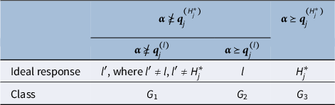
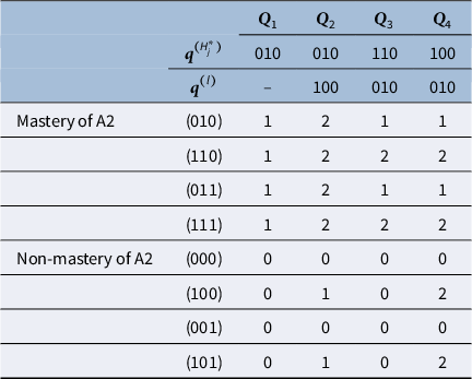
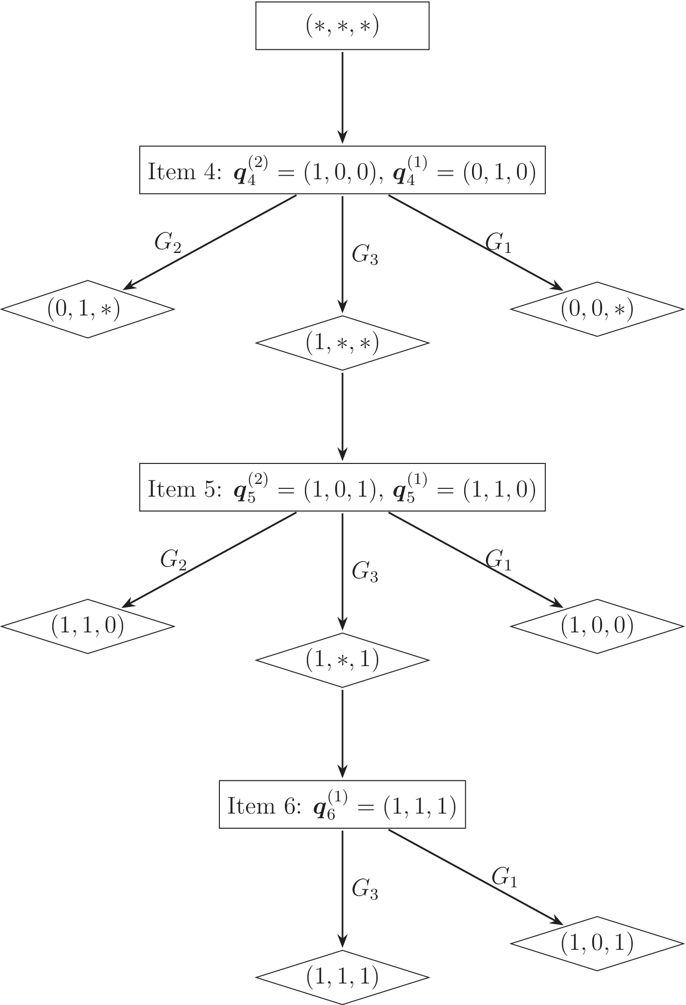
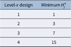

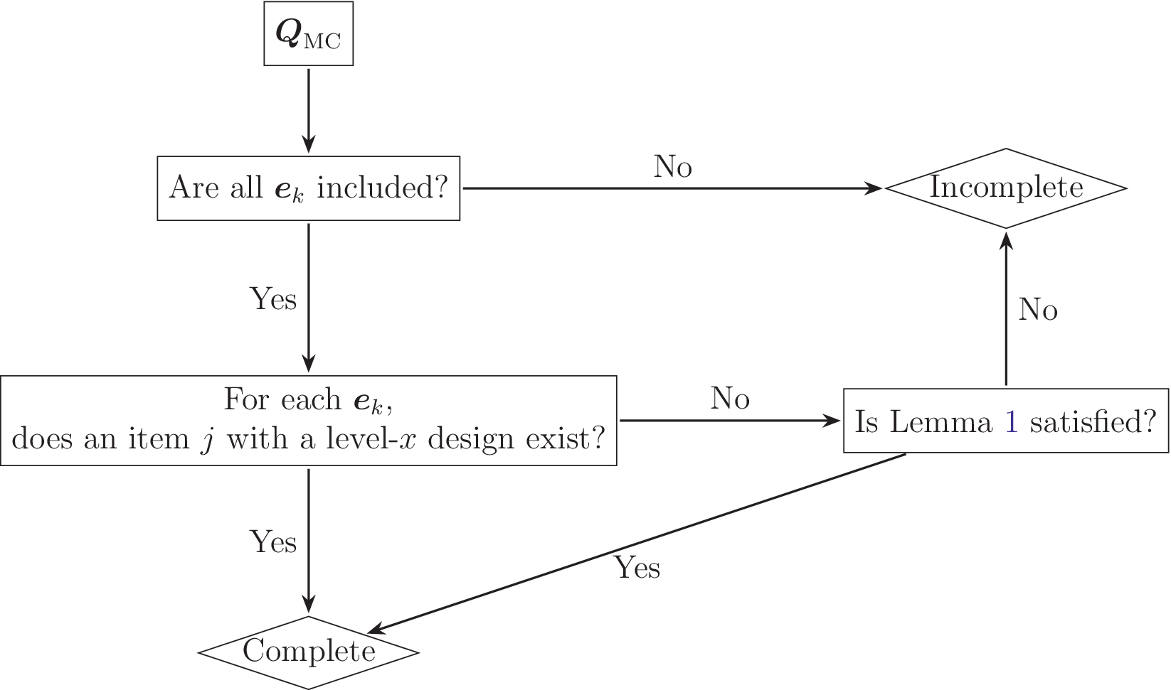

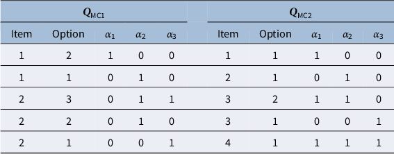


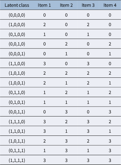


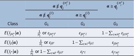


 Open access

