1 Introduction
The presence of a recirculation zone, which is common in jet engine combustion chambers, has a significant impact on flame dynamics, diverting the flame in large-scale motions and affecting its stability. Flame instabilities play an important role in combustion. They appear in different forms, under different flow regimes: in turbulent flows, in laminar flows and even quiescent surroundings. Some of the instabilities are related to intrinsic characteristics of the combustion thermo-diffusive process, in which hydrodynamics does not play a significant role. In his comprehensive review, Matalon (Reference Matalon2007) showed that flame instabilities, such as cellular structures and oscillating flames, appear in premixed as well as non-premixed diffusion flames. Due to the complexity of the configuration, non-premixed flames raise a challenge to be studied analytically. Moreover, the underlying hydrodynamics reported in experimental studies of diffusion flames usually involves multidimensional shear flows that directly influence the flame structure and stability (Matalon Reference Matalon2007). Due to these complicated flow structures, stability analysis of this flow is a formidable task.
Flame unsteadiness directly influences the combustion efficiency. The experimental studies of Owen, Spadaccini & Bowman (Reference Owen, Spadaccini and Bowman1976) have shown that pollutant emissions are sensitive to changes in operating conditions. Principal changes in the mean flow were found to occur in the initial regions of the combustion chamber, where initial mixing between the air and fuel streams occurs. In their experiment, significant large-scale fluctuations in the flame luminosity were observed for all test conditions, where the non-swirling flow exhibited the least stable flow conditions. Imposing swirl to the air stream reduced the flame fluctuations. Still, in all test conditions, the flames exhibited highly unsteady behaviour. Large-scale flame unsteadiness also appears in liquid spray combustion of the same configuration. Recently, Dagan, Arad & Tambour (Reference Dagan, Arad and Tambour2015) have numerically identified unique, two repetitive stages of a turbulent unsteady spray flame, developing in the vicinity of a recirculating flow. The complex flow regime diverts the fuel droplets and flame in periodic large-scale motions, bypassing the recirculation zone in the first stage and blocking it in the second stage.
For our present analyses, we chose the experimental data by Owen et al. (Reference Owen, Spadaccini and Bowman1976) since they are very comprehensive and very detailed for the geometrical configuration we chose to analyse. For the same reasons, Owen’s work has also served Pierce & Moin (Reference Pierce and Moin2001), Pierce & Moin (Reference Pierce and Moin2004) and Olbricht et al. (Reference Olbricht, Stein, Janicka, van Oijen, Wysocki and Kempf2012) in their studies of turbulent lifted flames.
1.1 Large eddy simulation of turbulent non-premixed combustion
The flow field in a combustion chamber is usually characterized by highly unsteady turbulent shear flows with moderate Reynolds numbers, where the effect of wall boundary layers is of secondary importance. Mixing and cooling processes, which significantly influence turbulent combustion, are governed by large-scale turbulent motions. This is the case where the advantages of large eddy simulations (LES) are most evident. In LES, these large-scale motions are fully resolved. Mongia (Reference Mongia2003) and Kim & Syed (Reference Kim and Syed2004) pointed out the importance of LES in designing advanced gas turbine combustion chambers. You, Ham & Moin (Reference You, Ham and Moin2008) have successfully conducted a LES analysis of turbulent combustion in a Pratt & Whitney gas turbine engine combustion chamber, handling a very complex geometry. Overall excellent agreement with experiments was reported. Their study provides the foundations for further research in which local unsteady flame dynamics can be investigated.
In the non-premixed combustion framework, heat release is mostly governed by the mixing intensity between the fuel and oxidizer (Peters Reference Peters1984). The mixing intensity can be characterized by the scalar dissipation rate. In order to maximize the heat release of combustion, rapid mixing between fuel and oxidizer is required, which corresponds to large values of the dissipation rate. However, local extinction can occur if the scalar dissipation rate exceeds a critical value over long periods (Ihme & Pitsch Reference Ihme and Pitsch2008). In this case, heat losses due to dissipation are of the order of magnitude of the heat release. This can lead to local reduction of the mixture temperature until flames locally extinguish. Reignition of the mixture is possible when the dissipation rate decreases and the temperature is raised by hot reactants transported to the locally premixed region. Hence, it is important to accurately predict scalar mixing in non-premixed combustion. Pitsch & Steiner (Reference Pitsch and Steiner2000) provided a comprehensive discussion of this subject. It was shown that a more accurate method significantly improves the prediction of reactive scalars, temperature and flow field variables.
A viable approach for accurately predicting the scalar mixing in LES is the steady laminar flamelet approach developed by Peters (Reference Peters1984). In this model, chemical reactions are assumed to be in balance with the rate of the reactants diffused into the flame. Therefore, the thermodynamic properties at the flame are evaluated as a function of the mixing rate which is characterized by the scalar dissipation rate. However, the flamelet’s solution results are in ambiguity while using the scalar dissipation rate (or mixture fraction) as a parameter. The transition from the burning to the non-burning solution is inevitably a discontinuous jump in flame state (Pierce & Moin Reference Pierce and Moin2004). Hence, local extinction and reignition cannot be properly predicted by the steady laminar flamelet model. In the current study, this ambiguity is resolved by using the flamelet-progress variable (FPV) approach developed by Pierce & Moin (Reference Pierce and Moin2004). In the FPV model, parameterization of the chemistry is performed by using both the mixture fraction and a reaction progress variable, rather than by the mixture fraction and scalar dissipation rate as used in the classical flamelet model approach of Peters (Reference Peters1984). Using this approach, Pierce & Moin (Reference Pierce and Moin2004) have successfully predicted flame lift-off in a confined combustor and validated their model by comparing mainly averaged quantities such as velocity, mixture fraction and product concentration fields to the experimental measurements of Owen et al. (Reference Owen, Spadaccini and Bowman1976).
The ability to predict local extinction and reignition effects using the FPV approach is discussed by Ihme, Chong & Pitsch (Reference Ihme, Chong and Pitsch2005), where good agreement with direct numerical simulation (DNS) computations was reported.
In the present study, we use a well-validated LES code package, CDP, from Cascade Technologies, Inc. This package has been successfully applied for the solution of large-scale turbulent combustion problems by Ham et al. (Reference Ham, Apte, Iaccarino, Wu, Herrmann, Constantinescu, Mahesh and Moin2003) and You et al. (Reference You, Ham and Moin2008).
1.2 Stability analysis of swirling jets subjected to recirculation
The evolution of instabilities in axisymmetric jets was comprehensively studied by Cohen & Wygnanski (Reference Cohen and Wygnanski1987a ,Reference Cohen and Wygnanski b ). Previous studies have been conducted on swirling flow instability of Poiseuille flow in a pipe subjected to non-parallel perturbations. Lessen, Sadler & Liu (Reference Lessen, Sadler and Liu1968) used asymptotic theories, and later, Khorrami, Malik & Ash (Reference Khorrami, Malik and Ash1989) used a Chebyshev collocation spectral method to solve several test cases of swirling flows. Olendraru & Sellier (Reference Olendraru and Sellier2002) addressed the viscous effects in the spatial instability of the Batchelor vortex. See & Ihme (Reference See and Ihme2014) have systematically investigated the effects of transport properties, and the effect of chemical reaction mechanisms, on the stability behaviour of a laminar jet diffusion flame. They show that the growth rate of the inviscid instability mode is insensitive to the representation of the transport properties at low frequencies. Stronger dependence on the mean flow representation was observed. Oberleithner et al. (Reference Oberleithner, Sieber, Nayeri, Paschereit, Petz, Hege, Noack and Wygnanski2011) have conducted a linear stability analysis for a flow with high swirl level, subjected to a central recirculation zone, as an outcome of vortex breakdown. Despite the complex flow considered, Oberleithner et al. (Reference Oberleithner, Sieber, Nayeri, Paschereit, Petz, Hege, Noack and Wygnanski2011) successfully applied a local spatial stability analysis to approximate the velocity of the global mode.
In the current study, we employ a temporal linear stability analysis, using a Chebyshev collocation spectral method in order to assess the contribution of hydrodynamic instability to the turbulent flame instabilities. The base flow for the present stability analysis is extracted from our time-averaged LES results. It should be noted that the theoretical linear stability analysis is valid for turbulent cases in which random fluctuations occur on a time scale that is short in comparison to the large-scale motions, which is the case for the large-scale flame motion analysed here. Using the linear stability approach, circumferential perturbations are shown to excite radial modes in the mixing region, providing an explanation for the significant correlation between circumferential and radial flame fluctuations.
1.3 Objective and outline
The objective of the present study is to analyse the behaviour of large-scale flame motions. We focus on turbulent gaseous flames, using LES, applied with the same configuration and flow conditions as those used in the experiment of Owen et al. (Reference Owen, Spadaccini and Bowman1976), incorporating swirling as well as non-swirling inflow conditions. The computational method employed here is validated using the comprehensive experimental database of Owen et al. (Reference Owen, Spadaccini and Bowman1976). Very good agreement of time-averaged results between the present numerical study and the experimental data was achieved, as shown here in § 4.
We use a new approach to quantify the flame homogeneity in the initial mixing region and to study its effect on the flame downstream evolution (§ 6). Using this method, unsteady phenomena reported by Owen et al. (Reference Owen, Spadaccini and Bowman1976) were observed here in our simulation. The three-dimensional evolution of the unsteady flame was analysed, revealing spatial downstream evolution of the large-scale quenched zones rotating continuously downstream about the axis while retaining a similar shape in the cross-section, even in non-swirling inflow conditions. Large-scale radial flame fluctuations were also identified and significant correlations between circumferential and radial flame frequencies were found.
A proper orthogonal decomposition (POD) approach and a semi-analytical linear stability analysis of the averaged flow field derived from the simulations are conducted. All three methods (flame tracking, POD and linear stability analysis) were then combined to illuminate the source of flame instability of the non-swirling case. From the POD analysis, the most energetic flame fluctuation modes were extracted. Using the linear stability model, these modes are shown to be the source of radial instability, which is directly connected to flame pulsation downstream. Remarkably, the flame fluctuation spectrum is predicted very well by the simple stability model derived here.
2 Computational method
2.1 Flow field equations
A well-validated LES code, developed at the Center of Turbulence Research (CTR) at Stanford University, was used in the current study. This code has been successfully applied for the solution of large scale turbulent combustion problems (see Ham et al. (Reference Ham, Apte, Iaccarino, Wu, Herrmann, Constantinescu, Mahesh and Moin2003) and You et al. (Reference You, Ham and Moin2008)).
The governing equations solved here are the unsteady, low Mach number filtered Navier–Stokes equations. The flow field variables are decomposed into resolved and subgrid-scale terms, by applying a grid-filtering operation. Small-scale fluctuations are removed by the filter, while their statistical effects remain in the residual terms of the filtered equations (Ferziger Reference Ferziger and Essers1983). For the subgrid-scale model, eddy viscosity and eddy diffusivities are evaluated using the dynamic Smagorinsky model, developed by Germano et al. (Reference Germano, Piomelli, Moin and Cabot1991). The filtered LES equations for continuity, momentum and scalar transport are,
 $$\begin{eqnarray}\displaystyle & \displaystyle \overline{\unicode[STIX]{x1D70C}}_{,t}+(\overline{\unicode[STIX]{x1D70C}}\tilde{\boldsymbol{u}_{j}})_{,j}=0, & \displaystyle\end{eqnarray}$$
 $$\begin{eqnarray}\displaystyle & \displaystyle (\overline{\unicode[STIX]{x1D70C}}\tilde{u_{i}})_{,t}+(\overline{\unicode[STIX]{x1D70C}}\tilde{u_{i}}\tilde{\boldsymbol{u}_{j}})_{,j}=-\overline{P}_{,i}+(2\overline{\unicode[STIX]{x1D707}}\tilde{S_{ij}})_{,t}+t_{ij}, & \displaystyle\end{eqnarray}$$
where
 $$\begin{eqnarray}\displaystyle \left.\begin{array}{@{}c@{}}\displaystyle \widetilde{S_{ij}}={\textstyle \frac{1}{2}}(\tilde{u} _{i,j})-{\textstyle \frac{1}{3}}\unicode[STIX]{x1D6FF}_{ij}\tilde{u} _{k,k},\\ \displaystyle t_{ij}=-\overline{\unicode[STIX]{x1D70C}}\widetilde{u_{i}\boldsymbol{u}_{j}}+\overline{\unicode[STIX]{x1D70C}}\tilde{u_{i}}\tilde{\boldsymbol{u}_{j}}=2\unicode[STIX]{x1D707}_{t}\tilde{S_{ij}}-{\textstyle \frac{1}{3}}\overline{\unicode[STIX]{x1D70C}}q^{2}\unicode[STIX]{x1D6FF}_{ij},\\ \displaystyle (\overline{\unicode[STIX]{x1D70C}}\tilde{\unicode[STIX]{x1D719}_{i}})_{,t}+(\overline{\unicode[STIX]{x1D70C}}\tilde{\boldsymbol{u}_{j}}\tilde{\unicode[STIX]{x1D719}_{i}})_{,j}=(\overline{\unicode[STIX]{x1D70C}}\tilde{\unicode[STIX]{x1D6FC}}\tilde{\unicode[STIX]{x1D719}_{i,k}})_{,k}+\overline{\unicode[STIX]{x1D70C}}\tilde{\unicode[STIX]{x1D714}}_{i}+q_{ik,k},\end{array}\right\} & & \displaystyle\end{eqnarray}$$
where
 $$\begin{eqnarray}\displaystyle q_{ik}=-\overline{\unicode[STIX]{x1D70C}}\widetilde{u_{k}\unicode[STIX]{x1D719}_{i}}+\overline{\unicode[STIX]{x1D70C}}\tilde{u_{k}}\widetilde{\unicode[STIX]{x1D719}_{i}}=\overline{\unicode[STIX]{x1D70C}}\unicode[STIX]{x1D6FC}_{t}\tilde{\unicode[STIX]{x1D719}}_{i,k} & & \displaystyle\end{eqnarray}$$
state relation:
 $$\begin{eqnarray}\displaystyle \overline{\unicode[STIX]{x1D70C}}=\overline{f(\unicode[STIX]{x1D719}_{1},\unicode[STIX]{x1D719}_{2},\ldots )}. & & \displaystyle\end{eqnarray}$$
Here,
 $\unicode[STIX]{x1D70C}$
is the density,
 $\boldsymbol{u}_{j}$
is the velocity vector,
 $p$
is the pressure,
 $\unicode[STIX]{x1D707}$
is the viscosity,
 $\unicode[STIX]{x1D6FF}_{ij}$
is the Kronecker symbol,
 $\unicode[STIX]{x1D719}_{i}$
represents a scalar quantity,
 $\unicode[STIX]{x1D6FC}_{i}$
is the diffusivity of scalar
 $i$
and
 $\unicode[STIX]{x1D714}_{i}$
is the chemical source term of scalar
 $i$
. The filtering operation is denoted by an overbar, and Favre (density weighted) filtering by a tilde. The unclosed transport terms in the momentum and scalar equations are: the residual stress
 $t_{ij}$
, residual scalar flux
 $q_{ik}$
, chemical source term
 $\tilde{\unicode[STIX]{x1D714}_{i}}$
and the turbulent diffusivity
 $\unicode[STIX]{x1D6FC}_{t}$
. These terms require a closure model. The state relation is reduced to an expression for density in terms of the transported scalars
 $\unicode[STIX]{x1D719}_{i}$
.
2.2 Chemical model
The FPV approach developed by Pierce & Moin (Reference Pierce and Moin2004) is utilized in the present study. In the FPV approach, a tabulated chemical table is computed in advance. Parameterization of the chemical properties is performed by using the mixture fraction, mixture fraction variance and a reaction progress variable. The conservation equations for the mixture fraction and progress variable scalars are
 $$\begin{eqnarray}\displaystyle & \displaystyle \frac{\unicode[STIX]{x2202}\overline{\unicode[STIX]{x1D70C}}\tilde{Z}}{\unicode[STIX]{x2202}t}+\unicode[STIX]{x1D735}\boldsymbol{\cdot }(\overline{\unicode[STIX]{x1D70C}}\tilde{u} \tilde{Z})=\unicode[STIX]{x1D735}\boldsymbol{\cdot }[\overline{\unicode[STIX]{x1D70C}}(\tilde{\unicode[STIX]{x1D6FC}}_{Z}+\unicode[STIX]{x1D6FC}_{t})\unicode[STIX]{x1D735}\tilde{Z}], & \displaystyle\end{eqnarray}$$
 $$\begin{eqnarray}\displaystyle & \displaystyle \frac{\unicode[STIX]{x2202}\overline{\unicode[STIX]{x1D70C}}\tilde{C}}{\unicode[STIX]{x2202}t}+\unicode[STIX]{x1D735}\boldsymbol{\cdot }(\overline{\unicode[STIX]{x1D70C}}\tilde{u} \tilde{C})=\unicode[STIX]{x1D735}\boldsymbol{\cdot }[\overline{\unicode[STIX]{x1D70C}}(\tilde{\unicode[STIX]{x1D6FC}}_{C}+\unicode[STIX]{x1D6FC}_{t})\unicode[STIX]{x1D735}\tilde{C}]+\overline{\unicode[STIX]{x1D70C}}\tilde{\unicode[STIX]{x1D714}}_{C}. & \displaystyle\end{eqnarray}$$
All the thermo-chemical properties, denoted by the vector
 $\unicode[STIX]{x1D733}$
, are parametrized in terms of the mixture fraction and the reaction progress variable:
 $$\begin{eqnarray}\displaystyle \unicode[STIX]{x1D74D}=\unicode[STIX]{x1D74D}(Z,C), & & \displaystyle\end{eqnarray}$$
where
 $\unicode[STIX]{x1D74D}=(T,y_{i},\dot{\unicode[STIX]{x1D714}}_{C},\unicode[STIX]{x1D70C},\unicode[STIX]{x1D708},\unicode[STIX]{x1D6FC})^{T}$
.
 $y_{i}$
is the mass fraction of species
 $i$
. The filtered thermo-chemical variables are obtained by integrating equation (2.8) over a joint probability density function (PDF). That way, subgrid fluctuations over the filtered chemical variables are incorporated.
 $$\begin{eqnarray}\displaystyle \widetilde{\unicode[STIX]{x1D74D}}=\iint \unicode[STIX]{x1D74D}(Z,C)\widetilde{P}(Z,C)\,\text{d}Z\,\text{d}C. & & \displaystyle\end{eqnarray}$$
The joint PDF is modelled by
 $$\begin{eqnarray}\displaystyle \widetilde{P}(Z,C)=P(C|Z)\widetilde{P}(Z). & & \displaystyle\end{eqnarray}$$
Here,
 $\widetilde{P}(Z)$
is given by the presumed beta PDF,
 $\unicode[STIX]{x1D6FD}(Z;\widetilde{Z},\widetilde{Z^{\prime \prime 2}})$
.
 $P(C|Z)$
is the conditional PDF which is represented by a delta function under the assumption that the scale over which a single flamelet is valid is greater than or equal to the size of the local computational cell, defined as follows:
 $$\begin{eqnarray}\displaystyle P(C|Z)=\unicode[STIX]{x1D6FF}(\widetilde{C}-C|Z), & & \displaystyle\end{eqnarray}$$
where
 $C\mid Z$
is given by the flamelet solution. The resulting state-space parametrization is a function of the mixture fraction, the mixture fraction variance and the reaction progress variable
 $\widetilde{\unicode[STIX]{x1D74D}}=\widetilde{\unicode[STIX]{x1D74D}}(\widetilde{Z},\widetilde{Z^{\prime \prime 2}},\widetilde{C})$
. The residual scalar variance of the mixture fraction can be written as
 $\widetilde{Z^{\prime \prime 2}}=\widetilde{Z^{2}}-\tilde{Z}^{2}$
. An additional transport equation is solved here for
 $\widetilde{Z^{2}}$
as this equation does not include a source term (Shunn & Moin Reference Shunn and Moin2009).
The flamelet libraries used in this study were computed for methane using GRI-Mech 2.11, a detailed kinetic mechanism containing 277 elementary chemical reactions and 49 species (Bowman et al. Reference Bowman, Hanson, Davidson, Gardiner, Lissianski, Smith, Golden, Frenklach and Goldenberg1995). The application of PDF methods for the approximation of reactive scalar subgrid fluctuations is comprehensively discussed by Ihme et al. (Reference Ihme, Chong and Pitsch2005). Using a DNS database for validation, Ihme et al. (Reference Ihme, Chong and Pitsch2005) have shown that the steady flamelet assumption in the context of the FPV approach, which is used here, leads to good predictions of local extinction and reignition.
It should be mentioned that, in principle, the non-premixed flamelet library used in the present flamelet-progress variable approach is not expected to predict the propagation of premixed branches of the lifted flames. However, what one can see in the present study configuration are mostly non-premixed large-scale flames, which are partially detached from the inlet and are stabilized by the swirling motion of the recirculation zone. Nevertheless, in the present cases, air is preheated to 750 K, suggesting that the entrainment of hot combustion products may not be sufficient to fully stabilize the flame, which then indicates the importance of partially premixed flame propagation in those regions.
Recently, See & Ihme (Reference See and Ihme2015) have shown that both the FPV framework, assuming steady flamelets, and a premixed-based filtered chemistry model provide good prediction of the highly unsteady flame dynamics of the German aerospace centre (DLR) dual swirl gas turbine model combustor (GMTC) which operates in the partially premixed combustion regime. In their configuration, the flame is lifted from the inlet. See & Ihme (Reference See and Ihme2015) also report a flame lifted from the inlet (in simulation and experiment). These results support the use of the current FPV model for the combustion regime of our configuration, which is mainly non-premixed and may involve local regions of partially premixed combustion and lifted flames. Further details on the application of the FPV approach can be found in the paper of Pierce & Moin (Reference Pierce and Moin2004).
2.3 Numerical method
The solution scheme formulates the discretized problem over a staggered mesh, where velocity components are staggered both in space and time. The challenge of capturing the turbulent structures responsible for the rapid mixing between fuel and oxidizer, while maintaining numerical stability, is met by the use of a non-dissipative, energy conserving scheme (Ham et al. Reference Ham, Apte, Iaccarino, Wu, Herrmann, Constantinescu, Mahesh and Moin2003). The time integration method is of second-order accuracy and fully implicit.
Neumann conditions for pressure and scalars were set as wall boundary conditions. No-slip Dirichlet conditions were applied for the velocity. Outflow boundaries were implemented using convective conditions.
A possible approach to accurately generate the combustor’s inflow conditions that fit the experiment (Owen et al. Reference Owen, Spadaccini and Bowman1976) is to completely resolve the turbulent flow in the configuration located upstream. This includes the wind tunnel ducts and swirl vanes. However, this is a very demanding task. A more practical approach, and the one used in the present study, was suggested by Pierce & Moin (Reference Pierce and Moin2004) as follows: inflow conditions are generated using a separated code, which simulates a fully developed, turbulent coaxial pipe flow. For the pipe simulation, spatially periodic boundary conditions are applied at the inlet and outlet of the pipe. Recycling is then used to establish fully developed, turbulent inflow conditions. Velocity cross-section data are sampled every few time steps and saved into an inflow database. The main combustion simulation uses this inflow database to generate the time-dependent fuel and air inlet boundary conditions. This approach is also used to simulate swirling inflow conditions.
3 Configuration and flow field
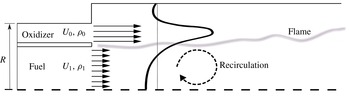
The combustion chamber configuration and flow conditions were set here to match the experimental study of Owen et al. (Reference Owen, Spadaccini and Bowman1976). The configuration under consideration is an axisymmetric, co-annular combustion chamber with two concentric inlet nozzles (figure 1). Combustion of air and gaseous methane is simulated, following Owen et al. (Reference Owen, Spadaccini and Bowman1976). The computational domain expands to
 $8R$
downstream from the inlet (37 % of the combustor length in the experiment). Fuel enters at 300 K through the inner inlet at a relative low speed of
 $U_{f}=1~\text{m}~\text{s}^{-1}$
and Reynolds number of:
 $Re_{R}=9669$
. The air enters at higher speed,
 $U_{a}=20.63~\text{m}~\text{s}^{-1}$
at 750 K and Reynolds number
 $Re_{R}=49\,219$
. The combustion chamber pressure is 3.8 atm. Flow variables were non-dimensionalized using the air inlet values. In the experiment (Owen et al.
Reference Owen, Spadaccini and Bowman1976), swirl was applied by partially diverting the air inflow using swirling vanes. The swirl number
 $S_{n}$
is defined as the ratio of angular momentum flux to axial momentum flux (Gupta, Lilley & Syred Reference Gupta, Lilley and Syred1984). Following Pierce & Moin (Reference Pierce and Moin1998), swirl velocity is imposed on the inflow field by implementing circumferential velocity in the upstream inflow generation code that was discussed in the previous section. Losses induced by individual vanes are not accounted for in the present simulation. In the experiment, the formulation for swirl number also included vane losses.
A schematic representation of the coaxial jet combustor configuration used in the present study and in the experimental set-up of Owen et al. (Reference Owen, Spadaccini and Bowman1976). Air and gaseous methane enter the combustion chamber separately from left to right in two co-annular pipes. Averaged axial velocity is illustrated here for clarity. The time-averaged axial velocity profile is schematically represented by the black curve. Dimensions:
 $R=0.047~\text{m}$
, fuel tube radius: 0.037 m and combustion chamber radius: 0.061 m.

4 Validation
4.1 Non-swirling conditions
Solution-mesh sensitivity tests for time-averaged velocity and temperature were conducted for the non-swirling case. It should be noted that a mesh-independence test is considered a challenging task in LES. Still, significant convergence has been achieved in most of the solution region and particularly in the flame region. Further details on the sensitivity tests conducted here can be found in appendix A.
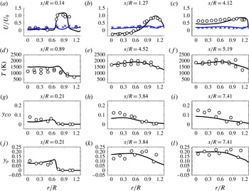
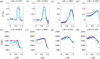
Radial profiles of time-averaged velocity, temperature, CO mass fraction and product mass fractions are compared with the experimental database (figure 2). Here, measurements that had been taken on the bottom half of the combustor were copied to the top half and presented in the radial range of:
 $r/R\in (0,1.3)$
.
Validation of the present computations. Non-swirling inflow (
 $Sn=0$
) time-averaged radial profiles of: (a–c) non-dimensional axial velocity, (d–f) temperature, (g–i) CO mass fraction and (j–l) product mass fraction. Experiment (Owen et al.
Reference Owen, Spadaccini and Bowman1976) ●, present computation ——. Velocity root mean square (RMS): experiment
 $\times$
(blue), computation — (blue).

The computed velocity profiles are in very good agreement with the measurements. As for the temperature, measured at the first two downstream stations, near the axis, our computation over-predicts the temperature by 300–400 K. This discrepancy in the upstream locations close to the inlet may also result from our combustion model which uses the non-premixed flamelet library and it may be that if one employs a partially premixed model, one would obtain a better fit of the computational results with the experimental data at upstream locations. However, the computed temperature profile is similar to the experimental profile. Furthermore, agreement at the external region (
 $r/R$
close to unity) is significantly better than near the axis.
In addition, as one may note, the measurements presented in the experimental study are scattered and hence cause some limitations to our model validation. However, as can be noted, in most cases our computational results appear to fall between the scattered experimental values; i.e. between the results measured in the upper radial location (
 $+r$
) of the combustor and the lower radial location (
 $-r$
) of the combustor, in this axisymmetric configuration. As will be shown here in § 5, large-scale motions of local quenched zones dominate the mixing region, travelling at low frequencies (below 2 Hz). Downstream, however, the flow stabilizes, and consequently, the agreement between the computation and experiment improves. Product mass fraction profiles are predicted well at all stations. CO mole fraction computational value is generally lower than the measured values at all four measurement stations. This is also the case in the computation of Pierce & Moin (Reference Pierce and Moin2004). Shunn & Moin (Reference Shunn and Moin2009) reported that using a more detailed model for the chemistry, which included convective heat loss, the prediction of CO mole fraction was improved. However, the use of the improved model only had a minor effect on the temperature field. The purpose of the current effort is to characterize the slowly evolving turbulent structures, which is accomplished through rigorous tracking of the temperature field. Thus, the present chemical model can be adequately applied here.
4.2 Swirl effect
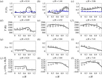
Time-averaged radial profiles of the thermo-chemical variables computed are shown in figure 3. The effect of swirl on the axial velocity (mean and RMS) is reconstructed very well at all downstream locations. Still, a local disagreement exists at
 $x/R=0.14$
at the peak velocity. Downstream, at locations
 $x/R=0.76,x/R=1.44$
, the swirl effect is twofold: higher axial velocities in the regions close to the combustor axis and a shift in the location of maximum axial velocity toward the combustor walls. This phenomenon is captured well by the present computation.
Swirling inflow (
 $Sn=0.3$
) time-averaged radial profiles of: (a–c) non-dimensional axial velocity, (d–f) temperature, (g–i) CO mass fraction and (j–l) product mass fraction. Experiment (Owen et al.
Reference Owen, Spadaccini and Bowman1976) ●, present computation ——. Velocity RMS: experiment
 $\times$
(blue), computation — (blue).
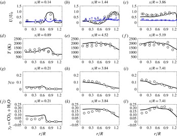
The level of agreement for CO mole fractions appears to be significantly better than the one observed in the non-swirling case at all cross-sections. Furthermore, better prediction of temperature profiles at the first two cross-sections is obtained for the flow with the inflow swirl. Product mass fractions are captured very well, except for regions close to the combustor’s axis. This result can be attributed to the fact that the swirl dominates the mixing in the flow field and its effect is well captured by the present model.
5 Flame structure and flame morphology
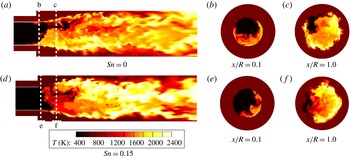
A highly non-symmetric flame structure develops for both swirling and non-swirling cases (figure 4). Local low temperature regions appear near the fuel inlet and change dynamically. These large-scale fluctuations had been observed in experiment (Owen et al. Reference Owen, Spadaccini and Bowman1976) and were later reported as highly unsteady flame lift-off (alternating its direction) in computation (Pierce & Moin Reference Pierce and Moin2004). Very similar flame structures were identified in an experimental study of free, non-swirling turbulent jets by Schefer (Reference Schefer1997).
Instantaneous snapshots of temperature distribution: (a–c) no inflow swirl
 $Sn=0$
, (d–f) swirl:
 $Sn=0.15$
. The distributions were extracted over a longitudinal cross-section cutting through the combustor’s centreline.

Qualitative comparison. (a–c) Computational cross-sections of instantaneous temperature distributions at different instances. (d–f) Experimental snapshots of
 $CH^{\ast }$
distributions representing the flame over a cross-section through jet. axial Jet velocity: 21
 $(\text{m}~\text{s}^{-1})$
(Schefer Reference Schefer1997).

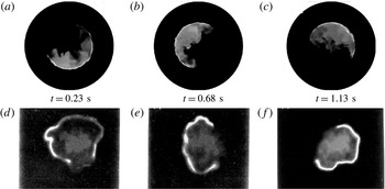
As one can see in the experimental results by Schefer, at each of the cross-sections, the circumferential flame is ‘dissected’ by darker areas with lower temperatures. Thus, we also analysed a few cross-section areas at various downstream locations and obtained similar behaviour of circumferential inhomogeneity (see figure 5
a–c). Axial cross-cuts of instantaneous temperature distributions are shown in figure 5 at several instances ranging from 0.23 to 1.13 s from ignition. The cross-section
 $x/R=0.1$
shown here is located just beyond the combustor inlet Non-uniformity in the turbulent flame structures is clearly observable in both sections. The computed temperature distributions in the cross-cuts are similar to the flow visualization snapshots from the experiment (Schefer Reference Schefer1997). In the experiment, the non-symmetric flame images presented in figure 5 were extracted using the
 $CH^{\ast }$
chemiluminescence method. As the flow conditions in Scheffer’s study were different from the present computation, this comparison is only qualitative. Nevertheless, both cases show a phenomenon of local quenching, which appears as a circumferential inhomogeneity in the flame structure, despite uniform inlet conditions. The time scale during which the quenching process takes place is related to the scalar dissipation evolution which contributes to the changes in size and shape of the quenched zone in somewhat stochastic manners.
Instantaneous snapshots of temperature in two cross-sections in the mixing region reveal a highly inhomogeneous flame for both swirling and non-swirling cases (figure 4
b,c,e,f). At the cross-section station:
 $x/R=0.1$
, most of the circular flame region is quenched, while at the time of ignition and shortly afterward, the whole circular region is burning homogeneously. The inhomogeneous condition develops only at later stages, suggesting a temporal instability developing close to the inlet. This temporal instability will be addressed in § 7.
Although significant flame oscillations were observed, large coherent structures rotating at a stable, constant rate were identified. These structures can be attributed to the phenomenon of precessing vortex core (PVC), described by Syred (Reference Syred2006). The PVC is a three-dimensional, time-dependent and large-scale coherent structure. According to Gupta et al. (Reference Gupta, Lilley and Syred1984), PVC depends on flow conditions as well as on the combustion process parameters and affects the swirling characteristics of the flow field.
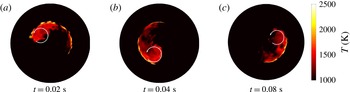
Temperature distributions in cross-section station
 $x/R=0.1$
, computed with inflow swirl of
 $Sn=0.3$
are displayed at different instances (figure 6). The coherent flame structures consist of a large main vortex (indicated by a white circle) followed by a thin wake located on the boundary between the air and the fuel, which takes approximately a quarter of the circumference. The entire structure rotates around the combustion chamber axis at a frequency of 12.5 Hz. In the following section, it will be shown that the rotation frequency is linearly correlated to the air inflow velocity magnitude.
Instantaneous temperature distribution snapshots reflecting a precessing vortex (indicated by white circle). Inflow swirl number:
 $Sn=0.3$
and cross-section at
 $x/R=0.1$
. Temperature snapshots were taken at three instances (measured from ignition):
 $t=0.03$
s (a),
 $t=0.04$
s (b),
 $t=0.05$
s (c).

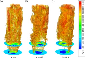
The effect of swirling inflow on the three-dimensional flame structure is shown via its influence on instantaneous isosurfaces of temperature (figure 7). Here, two isosurfaces of 2000 and 2300 K are displayed, capturing the important hot regions in the combustor. Detailed temperature distributions are shown for clarity on two axial downstream cross-sections:
 $x/R=0.1,1.0$
. Close to the inlets, at
 $x/R=0.1$
, flames take a slightly irregular, non-symmetric form and the effect of turbulent structures is apparent. When swirl (
 $Sn=0.15$
) is imposed at the inlet, significantly larger quenching regions appear. These regions expand even more when increasing the swirl number (to
 $Sn=0.3$
).
6 Coherent flame structures
6.1 Tracking functions formulation
Due to the complexity of turbulent flame evolution, the instantaneous three-dimensional flame structure is commonly presented graphically (e.g. Schefer Reference Schefer1997; Pierce & Moin Reference Pierce and Moin2004), in the same manner as displayed here in § 5. In the current study, we try to derive a quantitative characterization of the flame large-scale fluctuations. First, two-dimensional cross-sections of instantaneous snapshots of three-dimensional temperature distributions are extracted at each time step. Then, a set of one-dimensional functions is derived. This new approach provides a quantitative insight into the cross-section’s temporal flame evolution. The reduced functional representation lends itself to comparisons between flame evolution at different conditions.
Flame extinction and reignition regions were identified during the whole duration of the simulation. The quenched zone in the mixing region fluctuates in all directions. However, even in the case where no swirl was imposed on the inlet, large-scale motions of the quenched zone are identified in the azimuthal direction, which rotates about
 $180^{\circ }$
in less than one second (figure 5).
Isosurfaces of temperature: 2000 K (yellow) and 2300 K (red) at different swirl conditions: (a)
 $Sn=0$
, (b)
 $Sn=0.15$
and (c)
 $Sn=0.3$
. In addition, temperature distributions are shown at two axial downstream cross-sections:
 $x/R=0.1$
and
 $x/R=1.0$
.

It is suggested to track the quenched zone dynamics using the following formulation: the cross-sections are divided into sectors of a central angle
 $\unicode[STIX]{x1D719}$
, with variable circumferential angle
 $\unicode[STIX]{x1D703}$
, measured counterclockwise from the
 $x$
-axis to the bisector of each sector. The temperature field is scanned by rotating a sector counterclockwise, using small intervals of
 $\unicode[STIX]{x0394}\unicode[STIX]{x1D703}=0.01~\text{rad}$
, so that the whole circular cross-section is covered, allowing an overlap during the shifting process. A one-dimensional function is derived,
 $$\begin{eqnarray}\displaystyle \unicode[STIX]{x1D702}(\unicode[STIX]{x1D719},t)=\frac{\max (\bar{T}-\bar{T}_{\unicode[STIX]{x1D719}})}{\bar{T}}, & & \displaystyle\end{eqnarray}$$
which tracks the minimum temperature sector. The averaged sector temperature
 $\bar{T}_{\unicode[STIX]{x1D719}}$
is calculated for each sector of
 $\unicode[STIX]{x1D719}$
, where
 $$\begin{eqnarray}\displaystyle \bar{T}_{\unicode[STIX]{x1D719}}=\bar{T}_{\unicode[STIX]{x1D719}}(\unicode[STIX]{x1D719}_{1},\unicode[STIX]{x1D719}_{2})=\frac{\displaystyle \int _{\unicode[STIX]{x1D719}_{1}}^{\unicode[STIX]{x1D719}_{2}}\int _{0}^{R}Tr\,\text{d}r\,\text{d}\unicode[STIX]{x1D719}}{\displaystyle \int _{\unicode[STIX]{x1D719}1}^{\unicode[STIX]{x1D719}_{2}}\int _{0}^{R}r\,\text{d}r\,\text{d}\unicode[STIX]{x1D719}} & & \displaystyle\end{eqnarray}$$
and
 $\bar{T}=\bar{T}_{\unicode[STIX]{x1D719}}(0,2\unicode[STIX]{x03C0})$
is the average temperature over the entire cross-section.
 $\unicode[STIX]{x1D702}$
can also be used to evaluate the cross-section circumferential flame homogeneity as previously used by Dagan, Arad & Tambour (Reference Dagan, Arad and Tambour2011). As the sector rotates from
 $0$
to
 $2\unicode[STIX]{x03C0}$
, the computations of
 $\unicode[STIX]{x1D702}$
are employed to monitor the location of the minimum temperature sector:
 $\unicode[STIX]{x1D703}(\unicode[STIX]{x1D719},t)$
. Evaluation of cross-sections at various downstream locations, extracted from the current computational data base at multiple time steps, led to the selection of
 $\unicode[STIX]{x1D719}=60^{\circ }$
, as the most efficient section size for capturing the quenched zone. Furthermore, the dependency of
 $\unicode[STIX]{x1D703}(\unicode[STIX]{x1D719},t)$
on the size of the sector (
 $\unicode[STIX]{x1D719}$
) was found to be very weak. The parameter
 $\unicode[STIX]{x1D703}$
exhibits discontinuity for every
 $2\unicode[STIX]{x03C0}$
cycle. For presentation purposes, this undesirable behaviour can be avoided by the use of a functional representation:
 $\sin ^{2}(0.5\unicode[STIX]{x1D703})$
. As flame dynamics is the focus of the present study, a clear criterion to differentiate between self-sustained burning zones and extinguished zones is needed. A dichotomic-selection method was used for flame location. Using this criterion, for each computational cell, there is a dichotomic classification: unity (flame region) and zero (no flame). The threshold between burning and quenched zone was set at a temperature of 1800 K as follows.
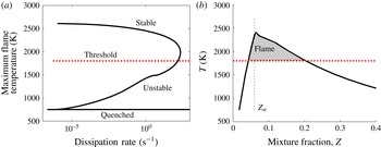
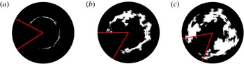
A flamelet solution which is employed by the current chemical model is presented in figure 8(a). The threshold of 1800 K was chosen to separate between a stable self-sustained branch and a non-stable or quenched flame. By doing so, we essentially define a flame thickness, which is on average rich in fuel, as can be seen in figure 8(b). Using the dichotomic representation, large locally quenched regions are automatically captured at three downstream cross-section stations:
 $x/R=0.1$
,
 $x/R=1.0$
and
 $x/R=2.0$
(figure 9).
(a) Maximum temperature as a function of the scalar dissipation rate, extracted from the present study flamelet solutions. A typical, three-branch s-curve is shown. The region above the chosen threshold of 1800 K represent the self-sustained, stable regions of the flame. (b) A flamelet solution (of the stable branch) with a dissipation rate of
 $\unicode[STIX]{x1D705}=1\times 10^{-5}~\text{s}^{-1}$
. The vertical dashed line represents the stoichiometric mixture fraction
 $Z_{st}$
. The shaded area represents the flame thickness, which in average is rich in fuel with
 $Z>Z_{st}$
.

Instantaneous flame distribution based on dichotomic selection at downstream stations: (a)
 $x/R=0.1$
, (b)
 $x/R=1.0$
and (c)
 $x/R=2.0$
. Flame region is displayed in white, computed at
 $t=3.45~\text{s}$
after ignition. No swirl condition:
 $Sn=0$
.
 $\unicode[STIX]{x1D702}(\unicode[STIX]{x1D719},t)$
criterion was applied to identify the quenched zones using
 $\unicode[STIX]{x1D719}=60^{\circ }$
. The resulting sectors are displayed by red lines.

In addition to the circumferential oscillations, radially pulsating flames were observed. A one-dimensional function that tracks the radial oscillations of the flame was used to analyse it. The temperature is extracted from a ring of width
 $\unicode[STIX]{x0394}r$
at a radius
 $r$
indicating the median of the ring. The radial location of maximum temperature of a downstream cross-section is extracted using
 $$\begin{eqnarray}\displaystyle \unicode[STIX]{x1D709}(\unicode[STIX]{x0394}r,r)=\frac{\max (\bar{T}_{\unicode[STIX]{x0394}r}-\bar{T})}{\bar{T}}, & & \displaystyle\end{eqnarray}$$
where
 $$\begin{eqnarray}\displaystyle \bar{T}_{\unicode[STIX]{x0394}r}=\frac{\displaystyle \int _{0}^{2\unicode[STIX]{x03C0}}\int _{r}^{r+\unicode[STIX]{x0394}r}Tr\,\text{d}r\,\text{d}\unicode[STIX]{x1D719}}{\displaystyle \int _{0}^{2\unicode[STIX]{x03C0}}\int _{0}^{R}r\,\text{d}r\,\text{d}\unicode[STIX]{x1D719}}. & & \displaystyle\end{eqnarray}$$
Here,
 $\unicode[STIX]{x1D709}$
represents the instantaneous radial temperature inhomogeneity of the flame radial location. The maximum temperature is tracked using a dichotomic tracking function
 $\unicode[STIX]{x1D701}(t)$
(with a threshold of 1800 K).
6.2 Application of the tracking functions
In order to build a database for the inhomogeneity analysis, the non-swirling and swirling cases, discussed in the previous sections, were solved to simulate 17.5 seconds of self-sustained combustion process. In the simulation, 770 000 time steps of
 $\unicode[STIX]{x0394}t=0.01R/U$
(a total non-dimensional time of
 $7700$
) were computed. For the flame tracking analysis, 77 000 samples of instantaneous temperature distributions were collected every tenth time step. Samples were extracted at cross-sections for three downstream locations along the combustion chamber’s axis:
 $x/R=0.1$
,
 $x/R=1.0$
,
 $x/R=2.0$
. The functions
 $\unicode[STIX]{x1D703}(\unicode[STIX]{x1D719},t)$
and
 $\unicode[STIX]{x1D701}(\unicode[STIX]{x1D719},t)$
were calculated over each cross-section. It was found that the circumferential level of homogeneity
 $\unicode[STIX]{x1D702}$
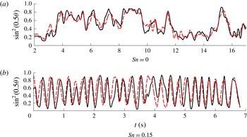
is kept constant throughout the simulation for the three cross-sections in the mixing region. The preservation of inhomogeneity level was reported by Dagan et al. (Reference Dagan, Arad and Tambour2011). Monitoring the dynamics of the circumferential flame location, the flame oscillates in a disordered manner into the non-burning zones, while additional burning zones quench. This phenomenon is captured in figure 10, which shows the temporal development of
 $\unicode[STIX]{x1D703}$
. The values of
 $\unicode[STIX]{x1D703}$
were low-pass filtered, by implementing a local regression using weighted linear least-squares for clarity. This method was chosen to preserve low frequencies as they reflect the spatial downstream evolution of the large-scale quenched zones which rotate downstream about the axis, and are the main focus of the current study.
Temporal development of the quenched region azimuth
 $\unicode[STIX]{x1D703}$
at two downstream stations: ——,
 $x/R=0.1$
and - - - -,
 $x/R=1.0$
for (a) non-swirling conditions, (b) low swirl of
 $Sn=0.15$
. Due to the periodic nature of the swirling case only a short time interval is presented. Time is measured from ignition.

Power spectral density of low-pass filtered
 $\unicode[STIX]{x1D703}(t)$
, extracted at cross-section station
 $x/R=1.0$
. Inflow swirl condition:
 $Sn=0.15$
. The most energetic frequency peak is denoted by
 $k_{p}$
.
 $k_{s}$
is the wavenumber representing swirl enforcement frequency. The red line represents the turbulent inertial slope of
 $k^{-5/3}$
.

A comparison between
 $\unicode[STIX]{x1D703}(t)$
spectra at different swirl conditions.
 $Sn=0$
(a–c),
 $Sn=0.075$
(d–f) and
 $Sn=0.15$
(g–i) at three downstream stations.
 $x/R=0.1$
(a,d,g),
 $x/R=1.0$
(b,e,h) and
 $x/R=2.0$
(c,f,i). Dominant frequency is indicated in the figure by
 $f_{p}$
.

It should be mentioned that the low-pass filter does not affect the results of the low flame frequencies. The low-pass filter is used here only to provide a clearer picture of the low frequencies.
For the non-swirling case, irregular dynamics of the quenched zone is clearly visible at the two stations of
 $x/R=0.1,1.0$
, in the proximity of the mixing region. The difference between the two cross-sections is negligible. This implies that instabilities originating near the inlet create a locally quenched zone which rotates. That way, the quenched zone along the combustor axis exhibits a solid-body rotation, preserving the same angle at different axial locations with similar temporal variations.
Flame dynamics in the case of a swirling inflow is very different than the non-swirling case discussed above. When swirl is imposed on the inlet, the flame moves periodically in a stable manner. The locally quenched zones, which resemble in shape and size those observed in the non-swirling case, swirl at a nearly constant rate (figure 10 b).
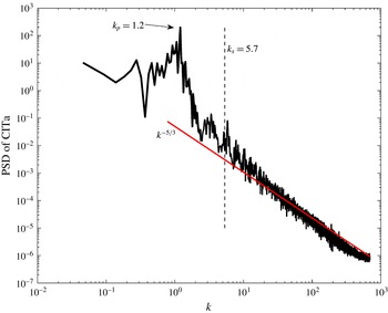
A power spectral density plot of the low-pass filtered
 $\unicode[STIX]{x1D703}(t)$
is shown in figure 11 for the case of swirling inflow
 $(Sn=0.15)$
. Here,
 $k=\unicode[STIX]{x1D714}/U_{0}$
is the wavenumber, where
 $\unicode[STIX]{x1D714}$
is the frequency (
 $\unicode[STIX]{x1D714}=2\unicode[STIX]{x03C0}f$
) and
 $U_{0}$
is a characteristic velocity, which is taken as the air inlet velocity. At the region of high wavenumber values, the slope of this spectrum is in agreement with the
 $k^{-5/3}$
slope that characterizes the turbulent inertial subrange. This indicates that the turbulent nature of the combustion is well captured by
 $\unicode[STIX]{x1D703}(t)$
. Several dominant low frequencies are observed. The most energetic one in the case of
 $Sn=0.15$
is
 $k_{p}=1.2$
. The wavenumber that represents the forcing swirl for this case is higher:
 $k_{s}=5.7$
. Hence, it appears that low-frequency modes of the circumferential flame dynamics are excited in the swirling cases.
It was found that the dominant frequency (
 $f_{p}$
) is linearly dependent on the air velocity magnitude
 $v$
, diverted by the angle
 $\unicode[STIX]{x1D6FD}$
, where
 $v=u/\text{cos}(\unicode[STIX]{x1D6FD})$
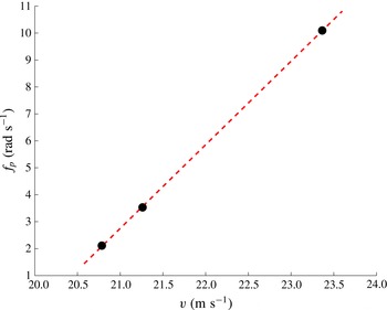
. A high linear correlation was found between
 $f_{p}$
and
 $v$
(figure 13). This correlation suggests that the rotation mode of the quench zone is directly influenced by the imposed inflow velocity at swirling conditions. This conclusion is consistent with the experimental results reported by Cassidy & Falvey (Reference Cassidy and Falvey1970) and appears also in Gupta et al. (Reference Gupta, Lilley and Syred1984), whereby for high Reynolds numbers, a frequency parameter
 $fD^{3}/Q$
was found to be independent of the Reynolds number and to increase linearly with the swirl number for swirl numbers higher than
 $0.3$
(where
 $f,D$
and
 $Q$
are the frequency of a PVC developed in a swirled flow, a reference diameter and the volumetric flow rate, respectively). However, for swirl numbers lower than
 $0.3$
,
 $fD^{3}/Q$
appears to be constant, and that is the range of swirl numbers that we are dealing with. Thus, for this regime, the frequency
 $f$
is a linear function of the volumetric flow rate
 $Q$
, and since
 $Q$
is directly proportional to the value of the inflow velocity
 $v$
, then the frequency
 $f$
should change linearly with
 $v$
at low swirl numbers, as we found in our study (see figure 13).
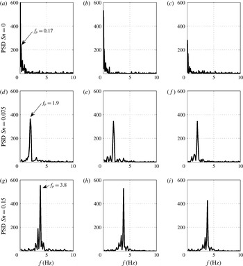
The swirling flows have significantly different spectra than the spectra of non-swirling flows. Furthermore, it is possible to characterize the influence of swirl on flame evolution for each swirling case. Focusing on the dominant frequencies of each case, a comparison between the spectra of three different low inflow swirl conditions:
 $Sn=0,0.075$
and
 $0.15$
is shown in figure 12. In the non-swirling inflow case, some dominant low frequencies (below 0.5 Hz) are evident. These frequencies do not change with the cross-section station downstream.
In addition to the fact that each of the swirling cases’ spectrum is dominated by a single frequency, it is less oscillatory than the non-swirling case’s spectrum. This insight is in agreement with the premise that the non-swirling flame evolution is a more chaotic process, as discussed in the previous section on time domain analysis.
Dominant computed frequency
 $f_{p}$
as a function of the diverted air velocity
 $v$
at swirl conditions:
 $Sn=0.075,0.15,0.3$
, respectively. The dashed line represents linear curve fitting between data points.

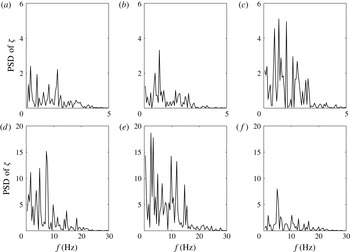
Power spectral density of the radial location of maximum temperature:
 $\unicode[STIX]{x1D701}$
, extracted at three downstream stations
 $x/R=0.1$
(a,d),
 $x/R=1.0$
(b,e),
 $x/R=2.0$
(c,f).
 $Sn=0$
(a–c),
 $Sn=0.15$
(d–f) (note that the abscissa and the ordinate in (a–c) are of a different scale than those in (d–f)).

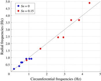
Correlation between the dominant frequencies of circumferential and radial oscillations of the flame, calculated at cross-section station:
 $x/R=0.1$
. Two inflow swirl conditions were tested:
 $Sn=0$
(blue) and
 $Sn=0.15$
(red). The dashed black line represent identity between circumferential and radial frequencies.

By tracking
 $\unicode[STIX]{x1D701}(t)$
it was possible to find the flame radial location and extract the pulsating characteristics of the flame. The pulsating motion of the flame starts as a sudden expansion outwards, thus rapidly consuming more of the oxidizer. As the stoichiometric ratio in this region is lost, the flame shrinks and the contact area of the fuel with the oxidizer reduces. This process keeps repeating itself. This flame instability is assumed to be triggered by the turbulent motion of the shear layer between the gaseous fuel and oxidizer, which modifies significantly the contact area.
For all the swirl levels that were investigated, radial fluctuation amplitudes were higher downstream, while minor fluctuations occur at the cross-section station in the mixing region (
 $x/R=0.1$
). On the other hand, large-scale circumferential fluctuations appear to be damped downstream (figure 12). Hence, it is suggested that circumferential oscillations are mostly affected by upstream fluctuations originating at the mixing region close to the inlet while radial fluctuation are excited mostly downstream.
Using the same practice as applied for the circumferential analysis discussed in the previous section, the spectra of radial flame locations for different swirling inflow conditions were computed at different cross-section stations (figure 14). For non-swirling conditions, a concentration of energy at low frequencies was observed. However, for swirl flow, it seems that this energy is dispersed upon a set of higher, distinct frequencies.
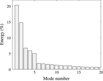
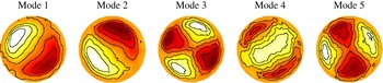
Spectrum of the POD temperature modes.

First five most energetic POD modes of temperature fluctuations. Modes are extracted for the non-swirling case (
 $Sn=0$
) at downstream location:
 $x/R=2.0$
.

It appears that the broad band of frequencies in the circumferential direction leaves its signature on fluctuation in the radial direction.
Analysing one-dimensional functions facilitates unique comparisons between different aspects of three-dimensional flame evolution. Such a comparison has been conducted between the flame’s circumferential fluctuations spectrum and the flame’s radial fluctuations spectrum using
 $\unicode[STIX]{x1D703}$
and
 $\unicode[STIX]{x1D701}$
spectra, respectively. While the spectra in the different directions (circumferential and radial) are different, a closer look at the most dominant radial and circumferential frequencies reveals a significant correlation which is presented in figure 15. Here, the
 $x$
-axis represents the circumferential leading frequencies and the
 $y$
-axis represents the radial dominant frequencies. Seven pairs of frequencies were collected for the non-swirling case (in blue) and seven for the swirling case (in red). The pairs were selected according to the most energetic frequencies (high power spectral density). Pearson coefficients were calculated for each case. The coefficients were
 $0.952$
for the non-swirling case and
 $0.9763$
for the swirling case, which indicates a high correlation between the pairs compared. The very high correlation of dominant frequencies indicates an interaction and transfer of energy between fluctuations in different directions. In the following sections, it will be shown that simplified representations of the flow field via proper orthogonal decomposition and linear stability analyses can reveal the onset of fluctuations and energy transfer between the circumferential and radial directions.
6.3 Proper orthogonal decomposition
A POD was utilized to further investigate the coherent flame structures. The POD analysis is used to extract low-order representations of a complex flow field by decomposing temporal, or spatial snapshot of flow field data into a set of orthogonal eigenfunctions. Commonly, POD is applied over the velocity field (Oberleithner et al. Reference Oberleithner, Sieber, Nayeri, Paschereit, Petz, Hege, Noack and Wygnanski2011). However, for the analysis of turbulent combustion, See & Ihme (Reference See and Ihme2014) found the temperature to be more informative. This approach is followed in the present study.
The eigenfunctions
 $\unicode[STIX]{x1D6E9}_{i}$
are calculated using the minimization of the mean square error between the temperature fluctuations
 $T(t,\boldsymbol{x})-\bar{T}(\boldsymbol{x})$
and the POD modes as follows:
 $$\begin{eqnarray}\displaystyle \min \left[\int \left((T(t,\boldsymbol{x}))-(\bar{T}(\boldsymbol{x}))-\sum a_{i}(t)\unicode[STIX]{x1D6E9}_{i}(\boldsymbol{x})\right)^{2}\,\text{d}\boldsymbol{x}\,\text{d}t\right]. & & \displaystyle\end{eqnarray}$$
The snapshot method (Sirovich Reference Sirovich1987) is applied here which extracts the most energetic structures and represents them as linear combinations. Since the large-scale turbulent structures usually contain the major portion of the energy, the POD modes with high-energy content are expected to span the basis for the dominant coherent structures.
The POD is employed on the computed data of the non-swirling case at three downstream cross-section locations:
 $x/R=0.1,1.0$
and
 $2.0$
. A set of 770 instantaneous temperature snapshots with a time increment of
 $0.0227~\text{s}$
were used for the POD analysis. Since the picture was very similar at all the analysed stations, we focus here on the most downstream cross-section location:
 $x/R=2.0$
. The most energetic modes are presented in figure 16. Over 50 % of the energy is contained in the first 5 most energetic modes. These modes are shown in figure 17. The first two modes contain over
 $35\,\%$
of the energy in the system and are also similar in shape and have a phase shift of
 $\unicode[STIX]{x03C0}/2$
, which clearly indicates a travelling azimuthal wave with a wavenumber of
 $m=1$
. Modes 3, 4 and 5 have twice the azimuthal wavenumber, having a phase shift of
 $\unicode[STIX]{x03C0}/4$
between them, therefore describing a travelling wave with a wavenumber of
 $m=2$
. Very similar modes have been identified by Oberleithner et al. (Reference Oberleithner, Sieber, Nayeri, Paschereit, Petz, Hege, Noack and Wygnanski2011) for swirling jets. This finding supports the claim that was raised in § 5: swirling-like rotations characterize the flame behaviour even in cases with zero inflow swirl. The fact that most of the energy is contained only in five simple azimuthal modes suggests that linear stability methods may be applied to investigate the large-scale dynamics of the flame.
7 Linear stability analysis
Temporal linear stability analysis is conducted here following the approach of Olendraru & Sellier (Reference Olendraru and Sellier2002) (details are provided here in appendix B). We assume a steady, axisymmetric base flow, superimposed by perturbations in the axial and circumferential directions. An eigenvalue problem is derived and solved for two cases. First, a temporal stability analysis of a Batchelor vortex is conducted here as a validation test case and very good results are obtained (see appendix B for further details). Then, a case of two concentric jets, which is a simplified model of the combustion chamber of the present study, is analysed. Although in the reacting LES solutions the density is changing and is not constant, in this case, the linear stability analysis is conducted for a base flow which was extracted from the time-averaged reacting LES solution, employing a constant density and is then carried out for the least stable linear stability modes.
7.1 Model formulation
In order to formulate the stability equations, the velocity is assumed to consist of a mean part and an infinitesimally small perturbation part, denoted here by
 $()^{\prime }$
:
 $$\begin{eqnarray}\displaystyle \left.\begin{array}{@{}c@{}}u=U+u^{\prime },\\ v=V+v^{\prime },\\ w=W+w^{\prime },\\ p=\unicode[STIX]{x03A0}+p^{\prime },\end{array}\right\} & & \displaystyle\end{eqnarray}$$
 $$\begin{eqnarray}\displaystyle \left.\begin{array}{@{}c@{}}U=U(r),\\ V=V(r),\\ W=W(r),\end{array}\right\} & & \displaystyle\end{eqnarray}$$
where
 $U$
,
 $V$
and
 $W$
are the axial, radial and tangential base-flow velocities, respectively. Following Olendraru & Sellier (Reference Olendraru and Sellier2002), the spectral collocation method for swirling base flows is described here, in which a ‘quasi-parallel’ base flow is assumed. The linear stability analysis is employed by superimposing on the base flow the disturbances in a modal decomposition form
 $$\begin{eqnarray}\displaystyle \{u^{\prime },v^{\prime },w^{\prime },p^{\prime }\}=Re\{H(r),\text{i}F(r),G(r),P(r)\}\text{e}^{\{\text{i}(kx+m\unicode[STIX]{x1D703}-\unicode[STIX]{x1D714}t)\}}, & & \displaystyle\end{eqnarray}$$
where
 $H$
,
 $F$
,
 $G$
and
 $P$
are the eigenfunctions,
 $k=k_{r}+\text{i}k_{i}$
is the complex axial wavenumber,
 $m$
is an integer azimuthal wavenumber and
 $w=w_{r}+iw_{i}$
is the complex frequency. By substituting the modal decomposition into the linearized Navier–Stokes equations and eliminating second-order terms we obtain the following linear system of equations:
 $$\begin{eqnarray}\displaystyle & \displaystyle F^{\prime }+\frac{F}{r}+\frac{mG}{r}+kH=0, & \displaystyle\end{eqnarray}$$
 $$\begin{eqnarray}\displaystyle & \displaystyle \frac{\text{i}F^{\prime \prime }}{Re}+\frac{\text{i}F^{\prime }}{rRe}-\left[\unicode[STIX]{x1D714}-\frac{mW}{r}-kU+\frac{\text{i}(m^{2}+1)}{r^{2}Re}\right]F-2\left[\frac{\text{i}m}{r^{2}Re}-\frac{W}{r}\right]G-P^{\prime }=\frac{\text{i}k^{2}F}{Re}, & \displaystyle \nonumber\\ \displaystyle & & \displaystyle\end{eqnarray}$$
 $$\begin{eqnarray}\displaystyle & \displaystyle \frac{G^{\prime \prime }}{Re}+\frac{G^{\prime }}{rRe}+\left[\text{i}\unicode[STIX]{x1D714}-\frac{\text{i}mW}{r}-\text{i}kU-\frac{m^{2}+1}{r^{2}Re}\right]G-\left[\text{i}W^{\prime }+\frac{2m}{r^{2}Re}+\frac{\text{i}W}{r}\right]F-\frac{\text{i}mP}{r}=\frac{k^{2}G}{Re}, & \displaystyle \nonumber\\ \displaystyle & & \displaystyle\end{eqnarray}$$
 $$\begin{eqnarray}\displaystyle & \displaystyle \frac{H^{\prime \prime }}{Re}+\frac{H^{\prime }}{rRe}+\left[\text{i}\unicode[STIX]{x1D714}-\frac{\text{i}mW}{r}-\text{i}kU-\frac{m^{2}}{r^{2}Re}\right]H-\text{i}U^{\prime }F-\text{i}kP=\frac{k^{2}H}{Re}. & \displaystyle\end{eqnarray}$$
Here,
 $()^{\prime }$
denotes derivation by
 $r$
.
Assuming no-slip boundary conditions at the walls,
 $$\begin{eqnarray}\displaystyle F(R)=G(R)=H(R)=P(R)=0. & & \displaystyle\end{eqnarray}$$
On the centreline, the requirement of single-valued perturbations imposes the following boundary conditions (Olendraru & Sellier Reference Olendraru and Sellier2002):
 $$\begin{eqnarray}\displaystyle \left.\begin{array}{@{}c@{}}F(0)=G(0)=H(0)=P(0)=0\quad \text{if }m>1,\\ H(0)=P(0)=0,\quad F^{\prime }(0)=G^{\prime }(0)=0\quad \text{if }m^{2}=1,\\ F(0)=G(0)=0,\quad H(0)\quad \text{and}\quad P(0)\quad \text{finite if }m^{2}=0.\end{array}\right\} & & \displaystyle\end{eqnarray}$$
For the temporal stability analysis, the system of equations is written in as a generalized eigenvalue problem
 $$\begin{eqnarray}\displaystyle \unicode[STIX]{x1D63C}\boldsymbol{X}=\unicode[STIX]{x1D714}\unicode[STIX]{x1D63D}\boldsymbol{X} & & \displaystyle\end{eqnarray}$$
for a discretized vector
 $\boldsymbol{X}=\boldsymbol{X}(\unicode[STIX]{x1D701})$
. For
 $N$
collocation points, matrices
 $\unicode[STIX]{x1D63C}$
and
 $\unicode[STIX]{x1D63D}$
are of the size
 $4\boldsymbol{N}\times 4\boldsymbol{N}$
. Using the Chebyshev derivative matrix
 $\unicode[STIX]{x1D63F}$
, we derive the expressions for matrices
 $\unicode[STIX]{x1D63C}$
and
 $\unicode[STIX]{x1D63D}$
, described in details in appendix B. A Chebyshev collocation approach was used in the present study, which simplifies the treatment of boundary conditions and distribute the numerical error in a homogeneous manner. For the case of concentric jets,
 $r$
varies between zero and
 $r_{max}=1$
. Thus, a transformation
 $$\begin{eqnarray}\displaystyle r=0.5(1-\unicode[STIX]{x1D701}), & & \displaystyle\end{eqnarray}$$
is used, which maps the Chebyshev interval
 $-1\leqslant \unicode[STIX]{x1D701}\leqslant +1$
onto the physical domain
 $0\leqslant r\leqslant 1$
.
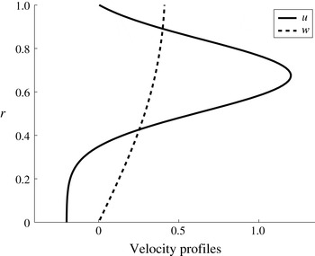
Time-averaged axial and circumferential base-flow velocity analytical profiles derived from LES results of the present study for a swirling case of
 $Sn=0.15$
.

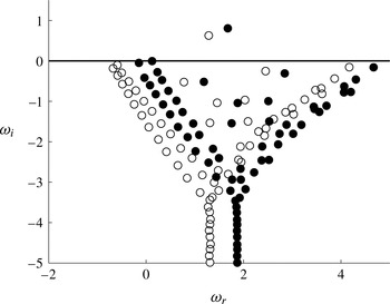
A typical eigenvalue map showing an unstable mode (
 $\unicode[STIX]{x1D714}_{i}>0$
). Calculated with circumferential wavenumber
 $m=1$
, axial wavenumber
 $k=3.6$
and two swirl parameters:
 $q=0$
(empty circles) and
 $q=0.65$
(filled circles), corresponding to swirl number of
 $Sn=0$
and
 $0.15$
in the simulation, respectively.

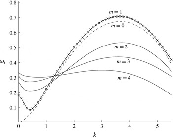
Growth rate represented as a function of the axial wavenumber
 $k$
for various helical modes
 $m$
for the non-swirling case (
 $q=0$
). The two most unstable modes are of wavenumbers
 $m=0$
and
 $m=1$
, denoted in
 $-\times -$
and dashed lines, respectively. Higher wavenumbers are presented in solid lines.

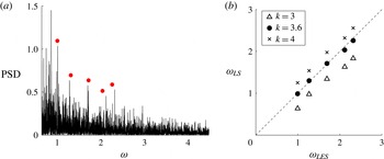
(a) Power spectral density of the radial flame fluctuations obtained from simulation (evaluated at
 $x/R=1.27$
). In red bullets, dimensionless frequencies obtained from the linear stability analysis
 $(k=3.6,m=0,1,2,3,4)$
; (b) correlations between the dimensionless frequencies obtained from simulation
 $(\unicode[STIX]{x1D714}_{LES})$
and the dimensionless frequencies obtained from linear stability analysis
 $(\unicode[STIX]{x1D714}_{LS})$
for
 $m=0,1,2,3,4$
and
 $k=3.6$
.

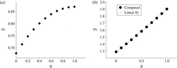
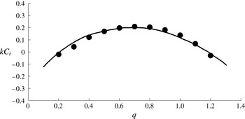
Variation of the least stable mode with swirl parameter
 $q$
. For this case,
 $k=3.6$
and
 $m=1$
, corresponding to maximum growth rate (figure 20).

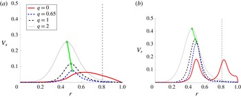
Variation of: (a) axial and (b) radial eigenfunctions profiles with the swirl parameter
 $q$
. Eigenfunctions were calculated for
 $Re_{s}=20\,000,m=5$
and
 $k=2$
. The case of
 $q=0.65$
correspond to swirl number
 $Sn=0.15$
in simulation. A linear connection between the eigenvalue peaks is shown in green line for
 $q>0$
.

7.2 Stability analysis of two concentric jets with back flow
The stability analysis is performed here for a case of two concentric jets shear flow with significant back flow, which represents the current study configuration. Unlike the full turbulent reacting case, a non-reacting, constant density, developed base flow is assumed. For the base flow, time-averaged axial and circumferential velocity profiles are extracted from the simulation, from which an analytical function is derived using least-squares functional fit as follows. For the axial velocity,
 $$\begin{eqnarray}\displaystyle U(r)=a_{0}\text{e}^{-b(cr-d)^{2}}-a_{1}, & & \displaystyle\end{eqnarray}$$
where
 $a_{0}=1.4,b=13,c=1.185,d=0.8$
and
 $a_{1}=0.2$
are constant coefficients. The circumferential velocity profile of the Batchelor vortex case § B.2,
 $$\begin{eqnarray}\displaystyle W(r)=q[1-\exp (-r^{2})]/r & & \displaystyle\end{eqnarray}$$
is used here as it represents a similar velocity curve, compared with the computed data for swirl parameters
 $q<2$
. This is a common approach to evaluate the least stable modes of swirling as well as non-swirling flows from experimental data (e.g. Oberleithner et al.
Reference Oberleithner, Sieber, Nayeri, Paschereit, Petz, Hege, Noack and Wygnanski2011). It should be noted that wavenumber growth rates might be weakly dependent on the location of the selected velocity profile. The purpose of this stability analysis is to gain physical insight into mechanism behind the onset of shear flow instabilities in the current configuration. Hence, a profile close to the inlet is considered. Profiles are shown in figure 18. The radial velocity profile is assumed to be zero. The velocity curves are extracted at axial downstream location:
 $x/R=1.27$
(see § 4, figure 2).
Since two concentric jets are considered, the characteristic velocity for the Reynolds number is defined as the velocity difference between the two jets
 $\unicode[STIX]{x0394}U$
. The Reynolds number for the stability analysis is therefore
 $$\begin{eqnarray}\displaystyle Re_{s}=\frac{\unicode[STIX]{x0394}UR}{\unicode[STIX]{x1D708}}, & & \displaystyle\end{eqnarray}$$
where
 $R$
is the outer cylinder radius,
 $\unicode[STIX]{x1D708}$
is the kinematic viscosity.
The eigenvalue map for both the non-swirling and swirling jet is shown in figure 19. One unstable eigenvalue (
 $\unicode[STIX]{x1D714}_{i}>0$
) was found. The growth rate for the non-swirling base-flow
 $(q=0)$
is shown in figure 20 for several circumferential wavenumbers as a function of the axial wavenumber
 $k$
. The maximum growth rate is obtained with wavenumber
 $m=1$
. For wavenumber
 $m=0$
, a slightly lower growth rate is obtained. As expected, these two modes are the least stable for most axial wavenumbers. It is obvious that the most significant point in the growth rate function is at the peak of the circumferential wavelength
 $m=1$
, which corresponds to the axial wavenumber of approximately
 $k=3.6$
(see figure 20). So by choosing the value of
 $k=3.6$
, we extracted the dimensionless frequency from our analytical stability analysis at
 $m=0,1,2,3,4$
. Next, by drawing the power spectral density for the radial flame fluctuations, one obtains figure 21(a). Then, by adding to figure 21(a) the points of radial frequencies obtained by our analytical stability calculations, one can clearly see that they fall in a very close vicinity of the computational peaks. This information appears also in figure 21(b), where we added wavenumbers
 $k=3$
and
 $k=4$
to show that at
 $k=3.6$
(about the maximum growth rate), the best match is obtained (with a Pearson correlation coefficient of 0.9980). It should be noted that some of the most dominant modes were not captured by this analysis, and specifically the most dominant mode:
 $\unicode[STIX]{x1D714}~0.6$
. Though simplified, these analytical results support the transfer of energy from circumferential and axial fluctuations to the radial fluctuations, giving insight into the mechanism of the onset of radial flame fluctuations in the real combustion chamber.
When swirl is considered (
 $q>0$
), the real wave frequency
 $\unicode[STIX]{x1D714}_{r}$
increases linearly with increase of the swirl parameter
 $q$
(figure 22
a). This is shown in figure 22 for
 $k=3.6$
and
 $m=1$
, corresponding to the least stable spatial mode of the non-swirling case. This is in agreement with the linear correlation found here in simulation (figure 13). On the other hand, the imaginary part of the frequency
 $\unicode[STIX]{x1D714}$
exhibits a nonlinear behaviour, sharply increasing in lower swirl parameters and reaching a plateau around
 $q=1$
(figure 22
b). A similar behaviour was observed in our validation test case with a Batchelor vortex (see appendix B for more details).
For non-swirling conditions (
 $q=0$
), axial and radial eigenfunctions are excited. These excitations occur for each test case studied here. However, the most significant effect on the radial fluctuations was found for the following combination of flow conditions:
 $m=5$
,
 $k=2$
and
 $Re_{s}=20\,000$
, which is shown in figure 23. In this specific case, the differences between non-swirling and swirling eigenfunctions are clear: for the axial eigenfunction, the non-swirling curve is diffused, while the swirling cases’ curves are narrow. A double-peak shape exists for the radial non-swirling case which is not evident when swirl is imposed. On the other hand, for increasing swirl parameters (
 $q>0$
), the eigenfunction peak magnitude is linearly increased, both in the axial and radial directions (figure 23). Since we introduced circumferential perturbations in the stability analysis which resulted in radial excitation of modes, especially in the shear layer region, one may expect that these energetic modes will be correlated with the circumferential modes. This phenomenon can explain the correlation between circumferential and radial fluctuations that was found in our computation of the turbulent case, where radial fluctuations were excited for increasing swirl numbers. Moreover, the most energetic frequencies excited are low compared with the typical turbulent inertial subrange frequencies (non-dimensional frequencies of the order of one). We may therefore suggest that the driving mechanism behind the frequency excitation is essentially laminar, as in the stability analysis performed here.
The use of different circumferential perturbation modes have also affected the eigenfunctions shape (figure 23). A double-peak eigenfunction was observed with
 $m=5$
in the radial eigenfunction at
 $r=0.82$
. In this case, the introduced swirl significantly changes the radial eigenfunction shape, and moves the axial velocity peak from
 $0.8$
, where the shear region is, towards the centre at
 $r=0.45$
. Radial fluctuations therefore affect the mixing between the two jets, especially in non-premixed combustion, where the chemical reaction is governed by mixing between fuel and oxidizer. We therefore expect that it also affects the flame’s evolution. Nevertheless, it should be mentioned that in order to accurately assess the effect of such a phenomenon, a full reactive flow stability analysis is required which is beyond the scope of our study.
8 Concluding remarks
The downstream evolution of a non-premixed, unsteady turbulent flame in a coaxial combustion chamber was analysed, employing LES. New dominant low flame frequencies were found. In addition to our LES studies we employed also harmonic analysis, POD and linear stability analysis. These essentially different methods allowed us to isolate and understand the driving mechanism behind the large-scale flame fluctuations that were studied in detail in our present research. Although the methods we employed here are different, they served us to portray a coherent picture of the physical insight of the unsteady behaviour of turbulent flame fluctuations in the radial, tangential and axial directions, for which we found new frequencies of these fluctuations which were not reported previously in the literature.
In the LES study, we were following computationally nearly 20 s of burning time for various inflow swirling conditions. Information regarding the flame behaviour at such long durations requires an extensive computational effort that was necessary in order to capture the large-scale motions of the unsteady flame.
After validating the computational approach with experimental data by Owen et al. (Reference Owen, Spadaccini and Bowman1976), we investigated new phenomena for unsteady, non-premixed turbulent flame structures. An automatic flame tracking method was introduced, providing the ability to track local quenched regions and analyse their dynamic evolution in time. Two criteria for characterizing flame structure were developed in the current study, providing the ability to quantify the overall spatial inhomogeneity in the combustor. The first one tracks the overall circumferential temperature inhomogeneity of a specific cross-section station perpendicular to the combustors axis. The second tracks radial inhomogeneity of the cross-section station. This toolkit, composed of one-dimensional functions, reduces the complexity of the three-dimensional, time-dependent phenomena and enables the quantification of flame inhomogeneity.
It was found here that a highly non-symmetric turbulent flame structure develops for both swirling and non-swirling cases. Local low temperature regions appear near the fuel inlet, ‘dissecting’ the circumferential flame and change dynamically. These regions were found to rotate continuously, even when non-swirling inflow conditions were imposed. Very similar flame structures were also identified in an experimental study of free, non-swirling turbulent jets by Schefer (Reference Schefer1997). In the non-swirling case, several dominant low rotational frequencies (below 2 Hz) were observed and endure downstream. The characteristic time scale of the flame itself i.e. the characteristic time of the chemical reaction, is definitely much shorter than the low frequencies observed in our study. The linear stability analysis which was conducted in our study reveals modes of low frequency which appear in the turbulent flow. These low-frequency modes, since they are the most energetic ones, naturally are expected to influence the low-frequency turbulent scales, and therefore influence the large-scale flame fluctuations. The source of the low-frequency fluctuations is attributed to interactions between the hydrodynamic fluctuations that affect the flame dynamics. The hydrodynamic stability analysis conducted here shows that one can predict the flame frequencies via the hydrodynamic frequencies.
The flame’s frequency spectrum reveals a typical turbulent spectrum modulated by these low frequencies. However, different phenomena appear when inflow swirl is imposed. Higher frequencies are then observed in a narrower frequency band. The spectra of the cases with imposed inflow swirl were found to be relatively smooth, with several low-frequency peaks. On the other hand, the spectrum of the case without inflow swirl exhibited multifrequency contribution. A linear correlation was found between the computed dominant frequency and the forcing inflow frequency. Radial flame pulsations were found to increase at downstream locations. This observation stands in contrast to the trend of circumferential fluctuations found here, which decrease as they advance downstream. Hence, energy is transformed between flame fluctuations in different directions.
One of the important findings in this study is the high level of correlation that was found between the frequencies of oscillations in the circumferential and radial directions. The inhomogeneity of the flame structure was extracted directly from the temperature field, but it is strongly coupled with the turbulent flow field. The azimuthal oscillation energy decays at cross-sections downstream along the combustor axis while radial oscillatory energy picks up at matching frequencies.
An empirical proper orthogonal decomposition method was conducted. Using POD, five rotational modes were found to contain most of the energy of the flame fluctuation in the mixing region. Finally, a theoretical linear stability method was derived and applied here for the present test case, extracting the velocity profiles from the time-averaged results of the detailed simulation. Using the linear stability model, these modes are shown to be the source of radial instability, which is directly connected to flame pulsation downstream, suggesting that the driving mechanism behind the frequency excitation is essentially laminar.
(a–d) Mesh dependence tests, using time-averaged, non-dimensional axial velocity. (e–h) Time-averaged temperature. Experiment (Owen et al.
Reference Owen, Spadaccini and Bowman1976):
 $\bullet$
.
 $128\times 64\times 32$
medium mesh: —— (blue),
 $256\times 150\times 64$
fine mesh: —— (red),
 $512\times 300\times 128$
extra fine mesh: —— (cyan).

These findings may have far reaching implications in the development of control strategies for combustion chamber efficiency and emission reduction.
Appendix A. Mesh sensitivity tests
Solution-mesh sensitivity tests were conducted using radial profiles of time-averaged axial velocity and temperature at four different cross-section stations along the combustion chamber axis for a non-swirling case. Three mesh refinement levels were tested: medium, fine and extra fine, consisting of 0.26 million, 2.5 million and 20 million hexahedral computational cells, respectively. Refinement focused on axial and circumferential directions, as the medium grid was relatively dense in the radial direction. Refinements were also implemented near the walls at
 $r/R=0.65$
and
 $r/R=1.0$
(inlet walls) and
 $r/R=1.2$
. The averaging time for statistics collection was the same at all grid refinements that were tested. The tests results are presented in figure 24, which also includes comparison with experimental results. Only marginal mesh dependency has been detected in the temperature profiles at regions very close to the inlets at radial locations of
 $r/R<0.65$
. As for the velocity profiles, mesh convergence has been achieved in all regions.
Appendix B. Linear stability equations formulation
In this section, the linear stability equations for two-dimensional base flow imposed by an axial and circumferential perturbations are derived. The governing equations for incompressible, viscous flows in axial, radial and azimuthal
 $(x,r,\unicode[STIX]{x1D703})$
cylindrical coordinates are,
continuity:
 $$\begin{eqnarray}\displaystyle \frac{\unicode[STIX]{x2202}u}{\unicode[STIX]{x2202}x}+\frac{1}{r}\frac{\unicode[STIX]{x2202}}{\unicode[STIX]{x2202}r}(rv)+\frac{1}{r}\frac{\unicode[STIX]{x2202}w}{\unicode[STIX]{x2202}\unicode[STIX]{x1D703}}=0; & & \displaystyle\end{eqnarray}$$
 $x$
-momentum:
 $$\begin{eqnarray}\displaystyle \frac{\unicode[STIX]{x2202}u}{\unicode[STIX]{x2202}t}+u\frac{\unicode[STIX]{x2202}u}{\unicode[STIX]{x2202}x}+v\frac{\unicode[STIX]{x2202}u}{\unicode[STIX]{x2202}r}+\frac{w}{r}\frac{\unicode[STIX]{x2202}u}{\unicode[STIX]{x2202}\unicode[STIX]{x1D703}}=-\frac{\unicode[STIX]{x2202}p}{\unicode[STIX]{x2202}x}+\frac{1}{Re}\left[\frac{1}{r}\frac{\unicode[STIX]{x2202}}{\unicode[STIX]{x2202}r}\left(r\frac{\unicode[STIX]{x2202}u}{\unicode[STIX]{x2202}r}\right)+\frac{1}{r^{2}}\frac{\unicode[STIX]{x2202}^{2}u}{\unicode[STIX]{x2202}\unicode[STIX]{x1D703}^{2}}+\frac{\unicode[STIX]{x2202}^{2}u}{\unicode[STIX]{x2202}x^{2}}\right]; & & \displaystyle\end{eqnarray}$$
 $r$
-momentum:
 $$\begin{eqnarray}\displaystyle & & \displaystyle \frac{\unicode[STIX]{x2202}v}{\unicode[STIX]{x2202}t}+u\frac{\unicode[STIX]{x2202}v}{\unicode[STIX]{x2202}x}+v\frac{\unicode[STIX]{x2202}v}{\unicode[STIX]{x2202}r}+\frac{w}{r}\frac{\unicode[STIX]{x2202}v}{\unicode[STIX]{x2202}\unicode[STIX]{x1D703}}-\frac{w^{2}}{r}\nonumber\\ \displaystyle & & \displaystyle \qquad =-\frac{\unicode[STIX]{x2202}p}{\unicode[STIX]{x2202}r}+\frac{1}{Re}\left[\frac{1}{r}\frac{\unicode[STIX]{x2202}}{\unicode[STIX]{x2202}r}\left(r\frac{\unicode[STIX]{x2202}v}{\unicode[STIX]{x2202}r}\right)-\frac{v}{r^{2}}+\frac{1}{r^{2}}\frac{\unicode[STIX]{x2202}^{2}v}{\unicode[STIX]{x2202}\unicode[STIX]{x1D703}^{2}}-\frac{2}{r^{2}}\frac{\unicode[STIX]{x2202}w}{\unicode[STIX]{x2202}\unicode[STIX]{x1D703}}+\frac{\unicode[STIX]{x2202}^{2}v}{\unicode[STIX]{x2202}x^{2}}\right];\end{eqnarray}$$
 $\unicode[STIX]{x1D703}$
-momentum:
 $$\begin{eqnarray}\displaystyle & & \displaystyle \frac{\unicode[STIX]{x2202}w}{\unicode[STIX]{x2202}t}+u\frac{\unicode[STIX]{x2202}w}{\unicode[STIX]{x2202}x}+v\frac{\unicode[STIX]{x2202}w^{\prime }}{\unicode[STIX]{x2202}r}+\frac{w}{r}\frac{\unicode[STIX]{x2202}w}{\unicode[STIX]{x2202}\unicode[STIX]{x1D703}}+\frac{vw}{r}\nonumber\\ \displaystyle & & \displaystyle \qquad =-\frac{1}{r}\frac{\unicode[STIX]{x2202}p}{\unicode[STIX]{x2202}\unicode[STIX]{x1D703}}+\frac{1}{Re}\left[\frac{1}{r}\frac{\unicode[STIX]{x2202}}{\unicode[STIX]{x2202}r}\left(r\frac{\unicode[STIX]{x2202}w}{\unicode[STIX]{x2202}r}\right)-\frac{w}{r^{2}}+\frac{1}{r^{2}}\frac{\unicode[STIX]{x2202}^{2}w}{\unicode[STIX]{x2202}\unicode[STIX]{x1D703}^{2}}+\frac{2}{r^{2}}\frac{\unicode[STIX]{x2202}v}{\unicode[STIX]{x2202}\unicode[STIX]{x1D703}}+\frac{\unicode[STIX]{x2202}^{2}w}{\unicode[STIX]{x2202}x^{2}}\right].\end{eqnarray}$$
B.1 Eigenvalue problem formulation
The generalized eigenvalue problem
 $\unicode[STIX]{x1D63C}\boldsymbol{X}=\unicode[STIX]{x1D714}\unicode[STIX]{x1D63D}\boldsymbol{X}$
is described here in details. Matrices
 $\unicode[STIX]{x1D63C}$
and
 $\unicode[STIX]{x1D63D}$
take the form
 $$\begin{eqnarray}\displaystyle \unicode[STIX]{x1D63C}=\left[\begin{array}{@{}cccc@{}}D+\displaystyle \frac{1}{r} & \displaystyle \frac{m}{r} & k & O\\ A_{21} & A_{22} & O & -D\\ A_{31} & A_{32} & O & -\displaystyle \frac{\text{i}m}{r}\\ -\text{i}U^{\prime } & O & A_{43} & -\text{i}k\end{array}\right],\quad \unicode[STIX]{x1D63D}=\left[\begin{array}{@{}cccc@{}}O & O & O & O\\ 1 & O & O & O\\ O & -\text{i} & O & O\\ O & O & -\text{i} & O\end{array}\right], & & \displaystyle\end{eqnarray}$$
where
 $$\begin{eqnarray}\displaystyle \left.\begin{array}{@{}c@{}}\displaystyle \unicode[STIX]{x1D608}_{21}=\frac{\text{i}D^{2}}{Re}+\frac{\text{i}D}{rRe}-\frac{\text{i}k^{2}}{Re}-\left[-\frac{mW}{r}-kU+\frac{\text{i}(m^{2}+1)}{r^{2}Re}\right],\\ \displaystyle \unicode[STIX]{x1D608}_{22}=-2\left[\frac{\text{i}m}{r^{2}Re}-\frac{W}{r}\right],\\ \displaystyle \unicode[STIX]{x1D608}_{31}=-\left[\text{i}W^{\prime }+\frac{2m}{r^{2}Re}+\frac{\text{i}W}{r}\right],\\ \displaystyle \unicode[STIX]{x1D608}_{32}=\frac{D^{2}}{Re}+\frac{D}{rRe}+\left(-\frac{\text{i}mW}{r}-\text{i}kU-\frac{m^{2}+1}{r^{2}Re}\right)-\frac{k^{2}}{Re},\\ \displaystyle \unicode[STIX]{x1D608}_{43}=\frac{D^{2}}{Re}+\frac{D}{rRe}+\left(\frac{\text{i}mW}{r}-\text{i}kU-\frac{m^{2}}{r^{2}Re}\right)-\frac{k^{2}}{Re}.\end{array}\right\} & & \displaystyle\end{eqnarray}$$
Here, matrices are diagonal of the size
 $\unicode[STIX]{x1D649}\times \unicode[STIX]{x1D649}$
and
 $O$
is a zero
 $\unicode[STIX]{x1D649}\times \unicode[STIX]{x1D649}$
matrix.
B.2 Validation: temporal stability of Batchelor vortex
In this section, the linear stability method is validated with the results of Khorrami et al. (Reference Khorrami, Malik and Ash1989) for a Batchelor vortex flow. The base-flow velocity profiles of a Batchelor vortex, consisting of axial and circumferential terms are
 $$\begin{eqnarray}\displaystyle \left.\begin{array}{@{}c@{}}U(r)=a+\exp (r^{2}),\\ V(r)=0,\\ W(r)=q[1-\exp (-r^{2})]/r,\end{array}\right\} & & \displaystyle\end{eqnarray}$$
where
 $q$
is a swirling parameter. Following Olendraru & Sellier (Reference Olendraru and Sellier2002), since
 $r$
varies between zero and infinity, a transformation is used
 $$\begin{eqnarray}\displaystyle \frac{r}{r_{c}}=(1+\unicode[STIX]{x1D702})\bigg/\left(1-\unicode[STIX]{x1D702}+\frac{2}{r_{max}}\right), & & \displaystyle\end{eqnarray}$$
which maps the Chebyshev interval
 $-1\leqslant \unicode[STIX]{x1D702}\leqslant +1$
onto the physical domain
 $0\leqslant \unicode[STIX]{x1D702}\leqslant r_{max}$
. By using this function, half of the collocation points are distributed in the interval
 $0\leqslant r\leqslant rc$
.
 $r_{max}=100$
and
 $r_{c}=3$
were used here as in the study of Olendraru & Sellier (Reference Olendraru and Sellier2002). The results of the present study were not sensitive to changes of these parameters (for values in the range:
 $2<r_{c}<4$
and
 $100<r_{max}<1000$
). Sensitivity tests were conducted for the number of collocation points.
Variation of the growth rate
 $kC_{i}$
with swirl parameter
 $q$
. The solid line represents results computed by Khorrami et al. (Reference Khorrami, Malik and Ash1989). The bullets the represent present computation.

Good agreement was obtained between the results of Khorrami et al. (Reference Khorrami, Malik and Ash1989) and the present computations (figure 25). It should be noted that Khorrami et al. (Reference Khorrami, Malik and Ash1989) had used a different transformation than the one used here and a different numerical scheme for solving the eigenvalue problem.