Vortex interaction between two tandem flexible propulsors with a paddling-based locomotion

Sung Goon Park; Hyung Jin Sung

doi:10.1017/jfm.2016.148

Vortex interaction between two tandem flexible propulsors with a paddling-based locomotion

Published online by Cambridge University Press: 18 March 2016

Sung Goon Park and

Hyung Jin Sung

Show author details

Sung Goon Park: Affiliation:
Department of Mechanical Engineering, KAIST, 291 Daehak-ro, Yuseong-gu, Daejeon 34141, Korea
Hyung Jin Sung*: Affiliation:
Department of Mechanical Engineering, KAIST, 291 Daehak-ro, Yuseong-gu, Daejeon 34141, Korea
*: †Email address for correspondence: hjsung@kaist.ac.kr

Article contents

Abstract
Introduction
Problem formulation
Results and discussion
Conclusions
Supplementary movie
References

Rights & Permissions

Abstract

Schooling behaviours among self-propelled animals can benefit propulsion. Inspired by the schooling behaviours of swimming jellyfish, flexible bodies that self-propel through a paddling-based motion were modelled in a tandem configuration. This present study explored the hydrodynamic patterns generated by the interactions between two flexible bodies and the surrounding fluid in the framework of the penalty immersed boundary method. The hydrodynamic patterns produced in the wake revealed flow-mediated interactions between two tandem propulsors, including vortex–vortex and vortex–body interactions. Two tandem flexible propulsors paddling with identical amplitude and frequency produced stable configurations as a result of the flow-mediated interactions. Both the upstream and downstream propulsors benefited from the tandem configuration in terms of the locomotion velocity and the cost, compared with an isolated propulsion system. The interactions were examined as a function of the initial gap distance and the phase difference in the paddling frequency. The equilibrium gap distance between two propulsors remained constant, regardless of the initial gap distance, although it did depend on the phase difference in the paddling frequency.

JFM classification

Biological Fluid Dynamics: Swimming/flying Vortex Flows: Vortex dynamics

Information

Type: Papers
Information: Journal of Fluid Mechanics , Volume 793 , 25 April 2016, pp. 612 - 632
DOI: https://doi.org/10.1017/jfm.2016.148 [Opens in a new window]
Copyright: © 2016 Cambridge University Press

1 Introduction

A variety of self-propulsion mechanisms used by animals that swim and fly through a fluid have been identified over the past several decades. The hydrodynamic patterns generated in the wake of a propulsor assist our understanding of propulsion mechanisms underlying the interaction between the propulsor and the surrounding fluid. The interaction process can be quite complex but intriguing. Many animals are flexible propulsors that exert forces on fluids via active body motions, while the surrounding fluid exerts a hydrodynamic force that determines the specific hydrodynamic patterns. Swimming fish form a thrust wake (or reverse von Kármán vortex street) by implementing an oscillating body motion that adds energy to the surrounding fluid (Ulrike Reference Ulrike2003). Jellyfish also transfer energy in the form of rotating masses in the surrounding fluid (Dabiri Reference Dabiri2005). An oblate jellyfish sheds wide vortical structures from the bell margin into the wake, whereas clear jet structures have been observed among prolate jellyfish (Colin & Costello Reference Colin and Costello2002). An analysis of the relevant hydrodynamic patterns has enabled deduction of the locomotive forces generated by propulsors (Dabiri Reference Dabiri2005). A study performed by Fish & Lauder (Reference Fish and Lauder2006) analysed the appendages of fish in relation to thrust production, manoeuvring and stability by measuring the hydrodynamic patterns present in the wake. Optimal vortex formation is related to energetics in gical propulsion (Linden & Turner Reference Linden and Turner2004; Dabiri Reference Dabiri2009).

Propulsors in a fluid generate wake structures through their propulsive action, and they occasionally exploit energetic structures in the surrounding fluid. A vertically flapping body in a viscous fluid generates a horizontal locomotion force through interactions with previously present vortical structures that exert hydrodynamic forces on a body (Alben & Shelley Reference Alben and Shelley2005). Fish can manipulate the surrounding fluid in both passive and active ways. The downstream fins can exploit the wake formed by the upstream fins in an individual fish with multiple fins (Lauder & Jayne Reference Lauder and Jayne1996; Fish & Lauder Reference Fish and Lauder2006). Liao et al. (Reference Liao, Beal, Lauder and Triantafyllou2003a ,Reference Liao, Beal, Lauder and Triantafyllou b ) showed that trout could extract energy from the upstream flow by altering their body kinematics and reducing muscle activity as they swim in the wakes of other objects. Eldredge & Pisani (Reference Eldredge and Pisani2008) simulated the behaviours of fish-like linked rigid bodies in the wake of a circular cylinder, revealing that the fish-like system could be passively propelled upstream without induced body undulations by obtaining thrust from the surrounding fluid. Jellyfish prolusion through the contraction and relaxation of the bell motions can act through a unique mechanism involving passive energy recapture. During the relaxation phase, positive pressure was generated beneath the bell by vortical structures that improved the cost of transport (Gemmell et al. Reference Gemmell, Costello, Colin, Stewart, Dabiri, Tafti and Priya2013). Wake recycling through vortex–vortex and vortex–body interactions has been observed in the schooling behaviours of many animals.

Fish schooling behaviours have been found by several researchers to involve the exploitation by downstream fish of vortices produced upstream. The downstream fish modulate their undulatory behaviours to reduce the cost of transport and resistance from flow (Belyayev & Zuyev Reference Belyayev and Zuyev1969; Weihs Reference Weihs1973; Breder Reference Breder1976). A detailed understanding of the mechanisms intrinsic to fish schooling has been sought through investigations of the vortex–vortex and vortex–body interactions using multiple flexible flags flapping passively in a uniform flow (Zhang et al. Reference Zhang, Childress, Libchaber and Shelley2000; Ristroph & Zhang Reference Ristroph and Zhang2008; Alben Reference Alben2009; Kim, Huang & Sung Reference Kim, Huang and Sung2010; Uddin, Huang & Sung Reference Uddin, Huang and Sung2013). Downstream propulsors in a tandem configuration encounter vortical structures that are shed from the leader and interact in complicated ways. Ristroph & Zhang (Reference Ristroph and Zhang2008) discovered that conventional drafting, in which a downstream body experiences drag reduction, only applies among rigid bodies and is not applicable to flexible bodies, such as swimming fish. Flexible filaments in a tandem configuration can experience inverted drafting, in which an upstream group enjoys drag reduction (Ristroph & Zhang Reference Ristroph and Zhang2008). Alben (Reference Alben2009) investigated the wake-mediated interactions between tandem flexible flags, revealing that inverted drafting occurs if the wake from the upstream flag adds constructively to the wake of the downstream flag. By contrast, certain gap distances between two flags promote drag reduction in a downstream flag if the wakes interact destructively (Alben Reference Alben2009; Kim et al. Reference Kim, Huang and Sung2010). Uddin et al. (Reference Uddin, Huang and Sung2013) investigated vortex–vortex and vortex–body interactions in systems of multiple flexible flags configured in triangular, diamond or conical configurations, revealing that the drag is affected by the interactions among the wakes. Although systems composed of passively flapping flags in a uniform flow significantly improve our understanding of the mechanisms that favour certain configurations in schooling behaviours, passive systems are limited in their applicability to fluid–body physics analysis because many propulsors are expected to interact with the surrounding fluid in both passive and active ways (Fish & Lauder Reference Fish and Lauder2006). Zhu, He & Zhang (Reference Zhu, He and Zhang2014) examined a system of self-propelled tandem flags in an effort to represent real world locomotion. Stable configurations formed spontaneously by locking up the trajectories onto vortex centres, thereby securing the energetic advantages of the follower.

Fish swim through the continuous flapping of their bodies, whereas jellyfish swim through the contraction and relaxation of the bell, leading to differences in the hydrodynamic patterns. Several studies have examined swimming jellyfish to analyse the wake structures that they produce during movement. Although jellyfish are jet-based propelling animals, a relatively small subset of jellyfish created a single vortex structure during a flapping cycle similar to the vortex structures produced by other animals during propulsion through jet-based locomotion (Dabiri Reference Dabiri2009). Many species generate different sets of vortical structures through the contraction and relaxation of the bell, and they interact with one another through a complicated mechanism (Colin & Costello Reference Colin and Costello2002; Dabiri Reference Dabiri2005; Sahin & Mohseni Reference Sahin and Mohseni2009; Park et al. Reference Park, Chang, Huang and Sung2014). Starting and stopping vortical structures were found to be generated during the contraction and relaxation phases, respectively, and the vortex induced motions in the surrounding fluid that were interrelated with the propulsion and feeding mechanisms (Colin & Costello Reference Colin and Costello2002; Mchenry & Jed Reference Mchenry and Jed2003; Dabiri et al. Reference Dabiri, Colin, Costello and Gharib2005; Sahin, Mohseni & Colin Reference Sahin, Mohseni and Colin2009; Park et al. Reference Park, Chang, Huang and Sung2014). Swarms of jellyfish are conspicuous in the oceans, but are not like synchronized schooling behaviours of swimming fish. Swarming jellyfish may be aggregated through active swimming, or they may drift together under wind or sea currents (Rottini Sandrini, Stravisi & Pieri Reference Rottini Sandrini, Stravisi and Pieri1980; Zavodnik Reference Zavodnik1987; Graham, Pages & Hamner Reference Graham, Pages and Hamner2001). The fact that jellyfish do not seem to swim in formations could be due to the lack of a sophisticated visual and sensory system not due to the absence in hydrodynamic benefits from schooling behaviours. As widely observed in swimming fish or flying birds, a hydrodynamic efficiency could be gained in the schooling behaviours of propulsors with a paddling-based locomotion, which is useful for the biologically inspired design and control of autonomous underwater vehicles.

The present study examined the dynamics of tandem flexible propulsors with an active paddling-based locomotion in a viscous quiescent flow. Although fish schooling behaviours and their hydrodynamic advantages have been widely studied, these are not applicable to the propulsors with a paddling-based locomotion due to the intrinsic differences in the flapping behaviours. Studies of two tandem flexible propulsors with a paddling-based locomotion and the resulting vortex–vortex and vortex–body interactions provide in-depth insight into vortex dynamics. The penalty immersed boundary method was used to consider the interactions between the propulsors and the surrounding fluid. Section 2 briefly describes the formulation and numerical methods. The numerical results and discussion are described in § 3. Finally, the study conclusions are presented in § 4.

2 Problem formulation

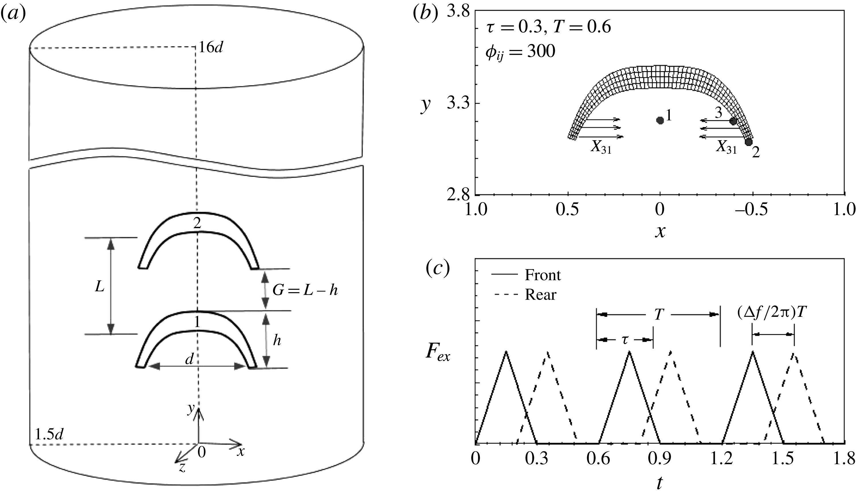
Figure 1(a) illustrates a schematic diagram of the tandem flexible propulsors and the coordinate system. The diameter and height of the flexible propulsors were denoted by $d$ and $h$ . The fineness ratio, defined by $h/d$ , was set to 0.4 in the present study, as shown in figure 1(a,b). $L$ indicates the gap distance between the centre positions of the two propulsors and $G$ is derived from the value of $L,G=L-h$ . 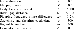The gap distance was adjusted through flow-mediated interactions over time. The fluid motion was defined on a fixed Eulerian grid system, whereas a separate moving Lagrangian grid system was applied to each flexible propulsor. The governing equations of the fluid and flexible propulsor motions were solved in each coordinate system in the framework of the immersed boundary method, in which the interactions were considered by adding feedback forces to each governing equation. The physical and numerical parameters are summarized in table 1.

Figure 1.

(a) Schematic diagram of two tandem swimming propulsors in a quiescent fluid and in a cylindrical computational domain. (b) Schematic diagram showing the propulsor bell, including the grid and the body force applied to the bell. Point 1 is on the centre axis and has the same $y$ location as point 3. Point 2 denotes the bell tip. Point 3 is the forcing point which satisfies the condition of the body force range in (2.9): ${\it\tau}=0.3$ , $T=0.6$ , ${\it\phi}=300$ . (c) The time histories of the body force. The solid and dashed lines denote the body forces on the front and rear propulsors, respectively.

Table 1.

Physical and numerical parameters.

The fluid motions were governed by the continuity and the incompressible Navier–Stokes equations in cylindrical coordinates,

(2.1)

$$\begin{eqnarray}\displaystyle & \displaystyle \frac{\partial \boldsymbol{u}}{\partial t}+\boldsymbol{u}\boldsymbol{\cdot }\boldsymbol{{\rm\nabla}}\boldsymbol{u}=-\boldsymbol{{\rm\nabla}}p+\frac{1}{Re}{\rm\nabla}^{2}\boldsymbol{u}+\boldsymbol{f}, & \displaystyle\end{eqnarray}$$

(2.2)

$$\begin{eqnarray}\displaystyle & \displaystyle \boldsymbol{{\rm\nabla}}\boldsymbol{\cdot }\boldsymbol{u}=0, & \displaystyle\end{eqnarray}$$

where

$\boldsymbol{u}$ is the velocity vector,

$p$ the pressure. The Reynolds number

$Re$ is defined by

$Re={\it\rho}_{0}u_{max}d/{\it\mu}$ , where

${\it\rho}_{0}$ is the fluid density,

$u_{max}$ is the maximum streamwise velocity,

$d$ is the diameter and

${\it\mu}$ is the dynamic viscosity. The Eulerian momentum force

$\boldsymbol{f}$ in (2.10) enables no-slip conditions along the immersed boundary.

The governing equation of a flexible propulsor is given by

(2.3)

$$\begin{eqnarray}{\it\rho}\frac{\partial ^{2}\boldsymbol{X}}{\partial t^{2}}=\boldsymbol{F}_{e}-\boldsymbol{F}_{l}+\boldsymbol{F}_{b},\end{eqnarray}$$

where $\boldsymbol{X}$ indicates the position, ${\it\rho}$ the density difference between the fluid and propulsor, $\boldsymbol{F}_{e}$ the elastic force, $\boldsymbol{F}_{l}$ the Lagrangian momentum force obtained as a result of the interaction with the surrounding fluid and $\boldsymbol{F}_{b}$ the body force required to deform the bell. The position $\boldsymbol{X}$ was defined using the Lagrangian variables $(s_{1},s_{2})$ on a moving curvilinear grid system to denote the position $\boldsymbol{X}$ , i.e. $\boldsymbol{X}(s_{1},s_{2},t)$ . The elastic force term $\boldsymbol{F}_{e}$ was derived from the variational derivative of the energy function. We assume that the elastic energy of the bell is

(2.4)

$$\begin{eqnarray}E(\boldsymbol{X})=\int _{{\it\Omega}_{s}}\unicode[STIX]{x1D652}_{s}\,\text{d}s_{1}\,\text{d}s_{2},\end{eqnarray}$$

where $\unicode[STIX]{x1D652}_{s}$ denotes the strain energy density. The strain energy density used in the present simulation was equivalent to the Skalak law neglecting the area dilation effect (Huang & Sung Reference Huang and Sung2009), which can be expressed in terms of the strain tensor

(2.5)

$$\begin{eqnarray}\unicode[STIX]{x1D652}_{s}={\it\phi}(\unicode[STIX]{x1D60B}_{11}^{2}+\unicode[STIX]{x1D60B}_{22}^{2}+2\unicode[STIX]{x1D60B}_{12}\unicode[STIX]{x1D60B}_{21}),\end{eqnarray}$$

where $\unicode[STIX]{x1D652}_{s}$ denotes the strain energy density and $\unicode[STIX]{x1D60B}_{ij}$ the Green strain tensor. The Green stain tensor is

(2.6)

$$\begin{eqnarray}\unicode[STIX]{x1D60B}_{ij}=\frac{1}{2}\left(\frac{\partial \boldsymbol{X}}{\partial s_{i}}\boldsymbol{\cdot }\frac{\partial \boldsymbol{X}}{\partial s_{j}}-\frac{\partial \boldsymbol{X}^{0}}{\partial s_{i}}\boldsymbol{\cdot }\frac{\partial \boldsymbol{X}^{0}}{\partial s_{j}}\right),\end{eqnarray}$$

where $\boldsymbol{X}^{0}$ stands for the initial position of the solid. The stress tensor can be obtained by $\partial \unicode[STIX]{x1D652}_{s}/\partial \unicode[STIX]{x1D60B}_{ij}$ , and takes the form of

(2.7)

$$\begin{eqnarray}{\it\sigma}_{ij}=2{\it\phi}_{ij}\unicode[STIX]{x1D60B}_{ij},\end{eqnarray}$$

where ${\it\sigma}_{ij}$ denotes the stress tensor and ${\it\phi}_{ij}$ indicates the stretching coefficient when $i=j$ and the shearing coefficient when $i\neq j$ . The stretching or shearing coefficient ${\it\phi}_{ij}$ was set to a value of 300, which is within the reasonable range of compressive stiffness measured by Megill (Reference Megill2002). The subscripts ‘ $i$ ’ and ‘ $j$ ’ indicate direction information in the propulsor body; ‘1’, ‘2’ and ‘3’ denote the longitudinal, transversal and circumferential directions, respectively. By using the variational derivative of the energy function, the elastic force can be described according to the following differential form:

(2.8)

$$\begin{eqnarray}\boldsymbol{F}_{e}=\mathop{\sum }_{i,j=1}^{3}\frac{\partial }{\partial s_{i}}\left({\it\sigma}_{ij}\frac{\partial \boldsymbol{X}}{\partial s_{j}}\right).\end{eqnarray}$$

The body force was applied to the bell to produce the bell motion of the flexible propulsor (Zhao, Freund & Moser Reference Zhao, Freund and Moser2008; Huang & Sung Reference Huang and Sung2009). $\boldsymbol{F}_{b1^{\prime }}$ and $\boldsymbol{F}_{b2^{\prime }}$ indicate the body forces on the rear and front propulsors, respectively

(2.9a )

$$\begin{eqnarray}\displaystyle & \displaystyle \boldsymbol{F}_{b1^{\prime }}=\left\{\begin{array}{@{}l@{}}\displaystyle {\it\alpha}|\boldsymbol{X}_{23}|\text{min}\left(t-\frac{{\rm\Delta}{\it\gamma}}{2{\rm\pi}}T,{\it\tau}-t+\frac{{\rm\Delta}{\it\gamma}}{2{\rm\pi}}T\right)\frac{\boldsymbol{X}_{31}}{|\boldsymbol{X}_{31}|},\\ \quad \quad \displaystyle |\boldsymbol{X}_{23}|<0.25,\frac{{\rm\Delta}{\it\gamma}}{2{\rm\pi}}T<t<{\it\tau}+\frac{{\rm\Delta}{\it\gamma}}{2{\rm\pi}}T,\\ \displaystyle 0,\quad \text{otherwise},\end{array}\right. & \displaystyle\end{eqnarray}$$

(2.9b )

$$\begin{eqnarray}\displaystyle & \displaystyle \boldsymbol{F}_{b2^{\prime }}=\left\{\begin{array}{@{}ll@{}}\displaystyle {\it\alpha}|\boldsymbol{X}_{23}|\text{min}(t,{\it\tau}-t)\frac{\boldsymbol{X}_{31}}{|\boldsymbol{X}_{31}|}, & \displaystyle |\boldsymbol{X}_{23}|<0.25,t<{\it\tau},\\ \displaystyle 0, & \text{otherwise},\end{array}\right. & \displaystyle\end{eqnarray}$$

where the subscripts ‘1’, ‘2’ and ‘3’ are the points described in figure 1(b),

${\it\alpha}$ indicates the body force coefficient,

${\rm\Delta}{\it\gamma}$ the phase difference in the flapping frequencies of the flexible propulsors,

$T$ is the flapping period and

${\it\tau}$ is the body force duration, as shown in figure 1(c).

$\boldsymbol{X}_{31}$ is the position vector from point 3 to point 1 and

$\boldsymbol{X}_{23}$ is from point 2 to point 3. In the present study,

${\it\alpha}$ ,

$T$ and

${\it\tau}$ were set to 5000, 0.6 and 0.3, respectively. The flexible propulsors and jellyfish have in common that the contraction behaviour is derived by the body force and the relaxation bell behaviour is obtained by the elastic energy stored in the bell during the contraction phase without an additional driving force. Parameters used in the body force are determined by trial and error to describe the bell motion of jellyfish (Park et al. 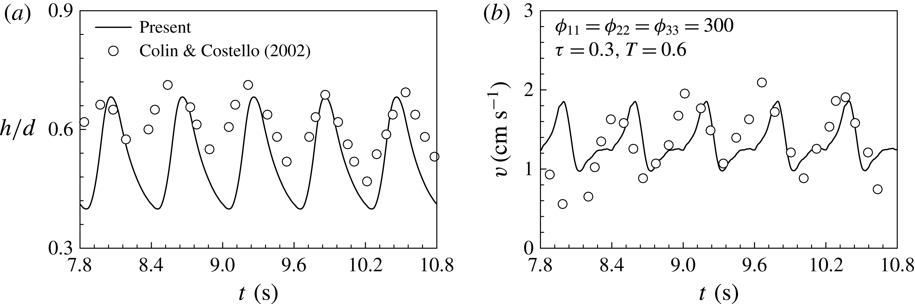2014). Figure 2(a,b) show time histories of the fineness ratio

$(h/d)$ and the centre velocity, respectively. The numerical results take a dimensional form for comparison with the experimental data (Colin & Costello 2002). The fineness ratio and the centre velocity show a similar trend to the experimental data.

Figure 2.

Time histories of (a) the fineness ratio and (b) the centre velocity.

The penalty immersed boundary method was used to reflect the interactions between the surrounding fluid and propulsors in the feedback momentum forcing terms $\boldsymbol{f}$ and $\boldsymbol{F}_{l}$ , which were added to each governing equation. Two sets of points on a Lagrangian grid were used; one set included the massless immersed boundary (IB) points $\boldsymbol{X}_{ib}$ , which directly interacted with the local fluid, and the other included the massive points $\boldsymbol{X}$ , which were obtained from (2.3). It was assumed that the massless points $\boldsymbol{X}_{ib}$ and the massive points $\boldsymbol{X}$ were linked via a spring with damping, by which the restoring force occurred when the IB points flowed with the local Eulerian fluid. The restoring force $\boldsymbol{F}_{l}$ added to (2.3), is given by

(2.10)

$$\begin{eqnarray}\boldsymbol{F}_{l}(s_{1},s_{2},t)=-{\it\kappa}[(\boldsymbol{X}_{ib}-\boldsymbol{X})+{\rm\Delta}t(\boldsymbol{U}_{ib}-\boldsymbol{U})],\end{eqnarray}$$

where ${\it\kappa}$ is a large constant used in Shin, Huang & Sung (Reference Shin, Huang and Sung2008), ${\rm\Delta}t$ is the computational time step, $\boldsymbol{U}_{ib}$ and $\boldsymbol{U}$ are the velocities of IB and the massive points, respectively. The Lagrangian restoring force was transformed into the Eulerian form using the smoothed Dirac delta function ${\it\delta}(\,)$ ,

(2.11)

$$\begin{eqnarray}\boldsymbol{f}(\boldsymbol{x},t)=\int _{{\it\Omega}_{S}}\boldsymbol{F}_{l}({\it\Gamma},t){\it\delta}(\boldsymbol{x}-\boldsymbol{X}({\it\Gamma},t))\,\text{d}s_{1}\,\text{d}s_{2},\end{eqnarray}$$

where ${\it\Omega}_{s}$ denotes the structure region and ${\it\Gamma}$ the structure boundary. The Eulerian momentum force was obtained. The fluid governing equations were solved using the fully implicit decoupling method (Kim, Baek & Sung Reference Kim, Baek and Sung2002) and the solid motion equation was solved using an iterative method. The detailed numerical procedures are described in Huang & Sung (Reference Huang and Sung2009) and Jang, Sung & Krogstad (Reference Jang, Sung and Krogstad2011).

3 Results and discussion

3.1 Numerical convergence

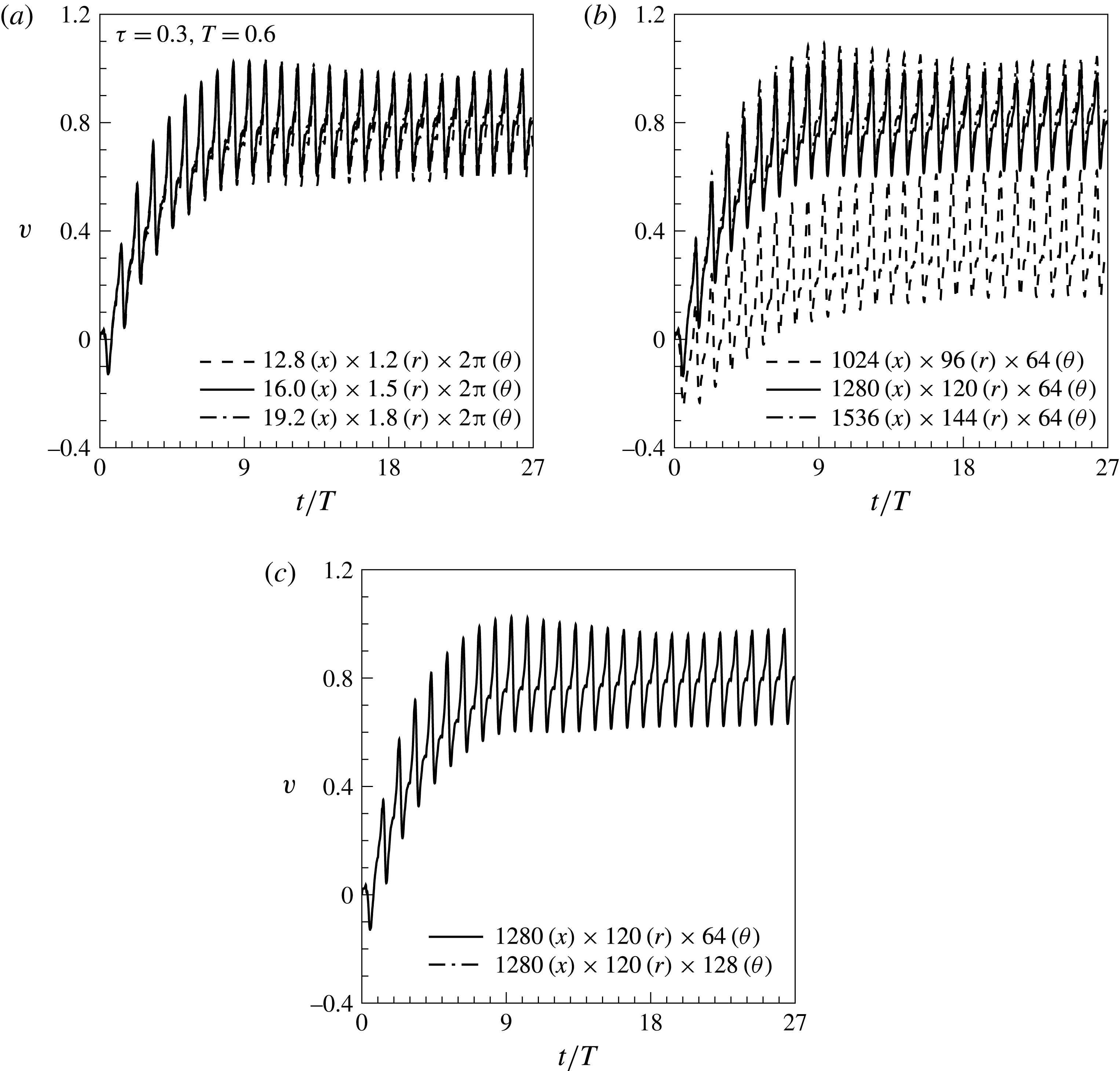
The computational domain sizes were 16.0, 1.5 and $2{\rm\pi}$ (1.5) in the longitudinal ( $x$ ), radial ( $r$ ) and azimuthal ( ${\it\theta}$ ) directions, respectively, and were normalized by the propulsor diameter. Figure 3(a) shows the time histories of the centre velocity, indicating that our computational domain size was sufficiently large. The Eulerian grid size was $1280\times 120\times 64$ in the longitudinal ( $x$ ), radial ( $r$ ) and azimuthal ( ${\it\theta}$ ) directions, respectively, and the Lagrangian grid size was $60\times 5$ . As shown in figure 3(b,c), the time histories of the centre velocity converged as the grid sizes in the $x$ - and $r$ -directions decreased, and were little affected by the grid size in the azimuthal direction. Few discrepancies were observed in the contraction and relaxation bell motions calculated over the different computational domain sizes and numbers of grids points. The Neumann boundary condition was applied at the fluid boundaries. The computational time step and $Re$ were set to 0.0001 and 400, respectively. For oblate swimming jellyfish, the Reynolds number was within the range of 100–700 (Colin & Costello Reference Colin and Costello2002).

Figure 3.

Time histories of the centre velocities over the different domain sizes (a), for different numbers of grids in the longitudinal and radial directions (b), and for different numbers of grid in the azimuthal direction (c).

3.2 Effects of the initial gap distance on the propulsion

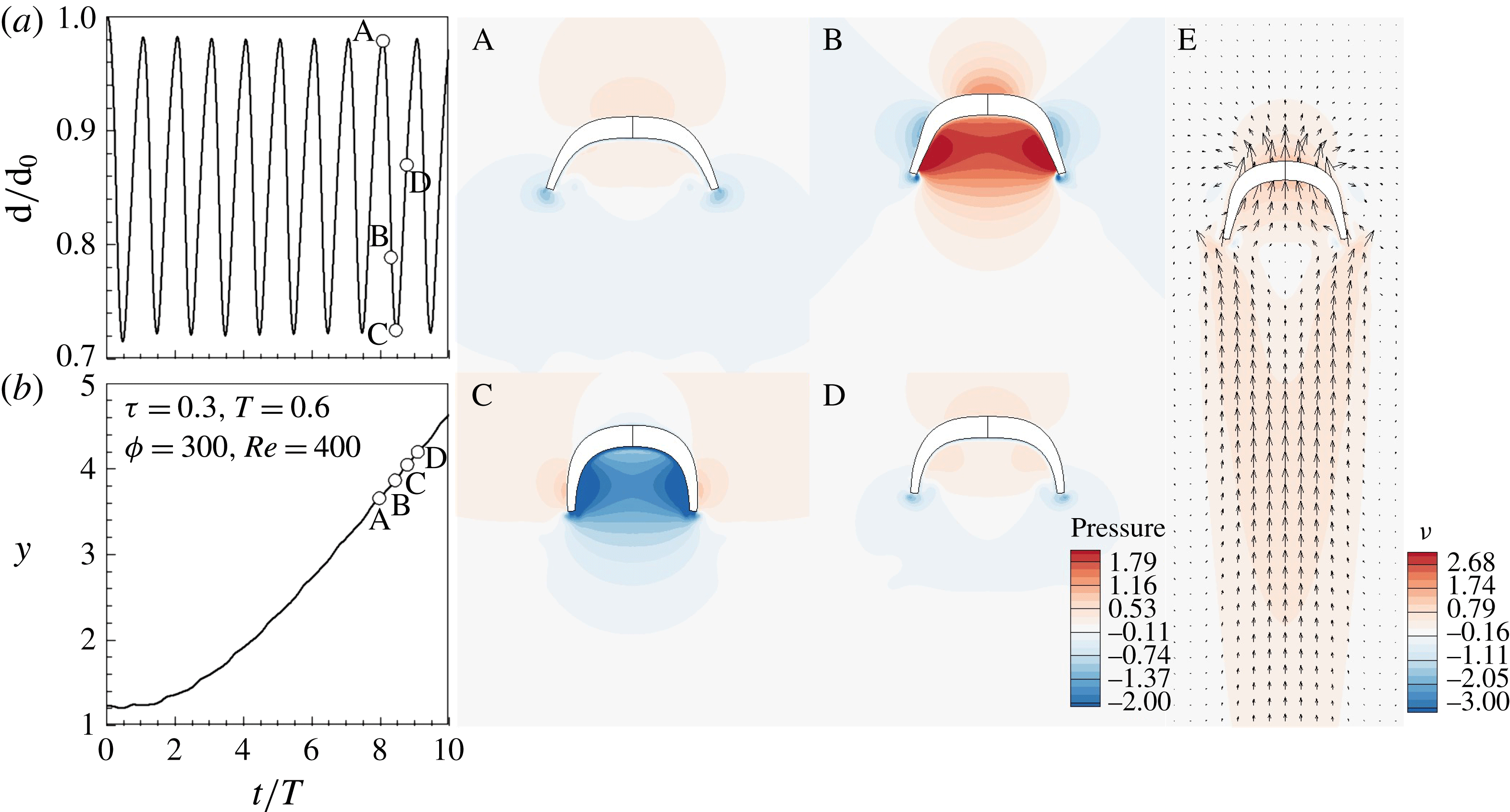
Before elucidating the hydrodynamic interactions between two tandem flexible propulsors with a paddling-based locomotion, an isolated propulsor was simulated to observe the swimming kinematics of the propulsor from the viewpoint of pressure variations near the propulsor. Figure 4(a) shows that the bell diameter decreased during the contraction phase and increased during the relaxation phase. Points A and C marked in figure 4(a,b) indicate the beginning and finishing of the contraction phase. In figure 4(b), the centre position of the propulsor in the moving direction increased to a lesser extent during the first two flapping periods, and then increased after the third flapping behaviour. At the instants of A–D, the pressure contours are displayed in figure 4. At the beginning of the contraction phase (A), the pressure in the upstream of the bell was larger than that measured inside of the bell. During the early stage of the contraction phase (A–B), the bell deformed rapidly, increasing the pressure inside of the bell. As the contraction phase proceeded (B–C), the bell deformation rate decreased, leading to the decreased pressure inside the bell (C). As the relaxation phase proceeded, the surrounding fluids were injected into the inside of the bell and the pressure measured inside of the bell increased during the relaxation phase (D). The velocity vectors surrounding the propulsor in the midst of the contraction phase are displayed in E. A weak hole induced by the contraction is observed in the near wake region (E). Beyond this region, the flow velocity increased in the moving direction. Beal et al. (Reference Beal, Hover, Triantafyllou, Liao and Lauder2006) found that the drag force behind a bluff body is smaller than that in open flow due to the reduced relative velocity between fish and the surrounding fluid. The propulsor behind another propulsor also experienced the reduced relative velocity as compared to the propulsor moving in a quiescent fluid due to the increased flow velocity in the moving direction (E).

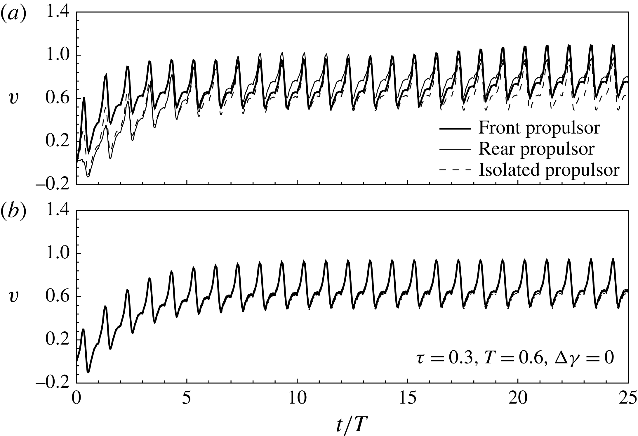
Figure 5(a) shows the time history of the centre velocity for an isolated swimming propulsor (IP) and each propulsor in a tandem configuration for an initial gap distance $G_{o}$ of zero. The velocity profiles increased during the initial flapping periods, then converged. In the tandem configuration with a small initial gap distance ( $G_{o}=0$ ), the front flexible propulsor (FP) moved faster than the rear propulsor (RP) during the initial flapping periods because RP experienced an increase in drag from the upstream flow, as shown in figure 5(a). In the steady state, both FP and RP were faster than IP, suggesting that propulsion in a tandem configuration was more beneficial than isolated propulsion, with respect to the propulsion velocity. The ratios of velocity fluctuations to mean velocity in swimming eels and mullets showed 4 % (Tytell & Lauder Reference Tytell and Lauder2004) and 20 % (Muller et al. 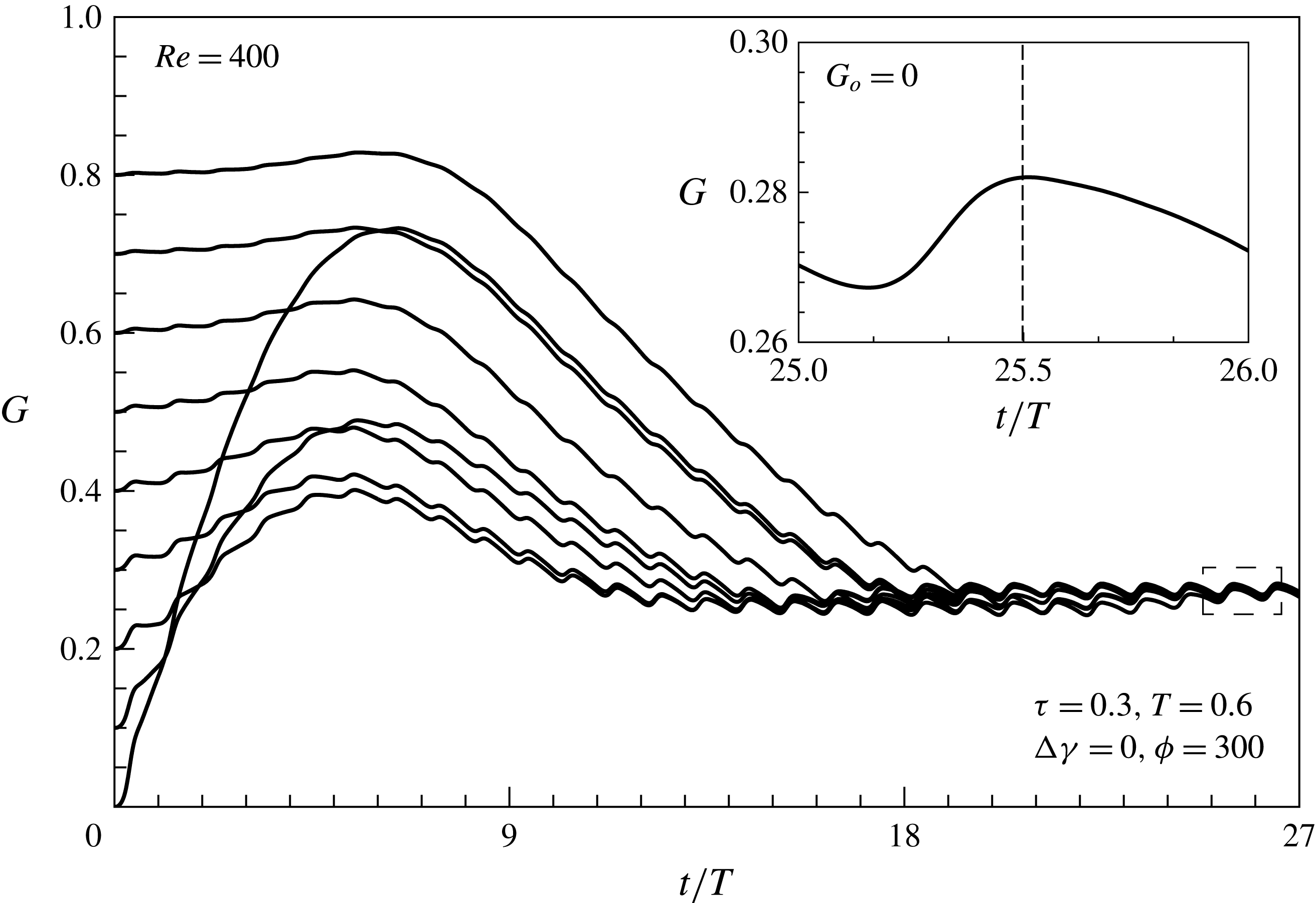Reference Muller, van den Heuvel, Stamhuis and Videler1997), respectively. These were attributed to the differences of the body shape and the swimming kinematics of the propulsors (Borazjani Reference Borazjani2015). In figure 5(a), FP, RP and IP exhibit 21 %, 36 % and 38 % of velocity fluctuations, respectively. This means that the velocity fluctuations are also influenced by the surrounding fluid. Figure 5(b) shows the centre velocities of the FP and RP in a tandem configuration for an initial gap distance of 6, similar to the centre velocity of IP, indicating that an upstream wake did not significantly affect RP for large gap distances between FP and RP. Figure 6 shows the time histories of the gap distances between FP and RP for different initial gap distances. The phase difference in the flapping frequency was set to zero. In a tandem configuration, FP and RP reached a stable configuration in which the gap distance converged to approximately 0.27, regardless of the initial gap distance, as shown in figure 6. The initial gap distance influenced the time required to reach a stable configuration, but it did not influence the equilibrium positions. In the stable configuration, the gap distance between FP and RP increased and decreased during the contraction and relaxation periods, respectively.

Figure 4.

Time histories of (a) the normalized diameter and (b) the centre position in the moving direction and the pressure contours at A $(t/T=8)$ , B $(t/T=8+2/6)$ , C $(t/T=8+3/6)$ and D $(t/T=8+4.5/6)$ . Velocity contour in the moving direction at E $(t/T=8+2/6)$ .

Figure 5.

Time histories of the centre velocity. (a) $G_{o}=0$ , $Re=400$ , (b) $G_{o}=6$ .

Figure 6.

Time histories of the gap distance between the tandem propulsors for different initial positions.

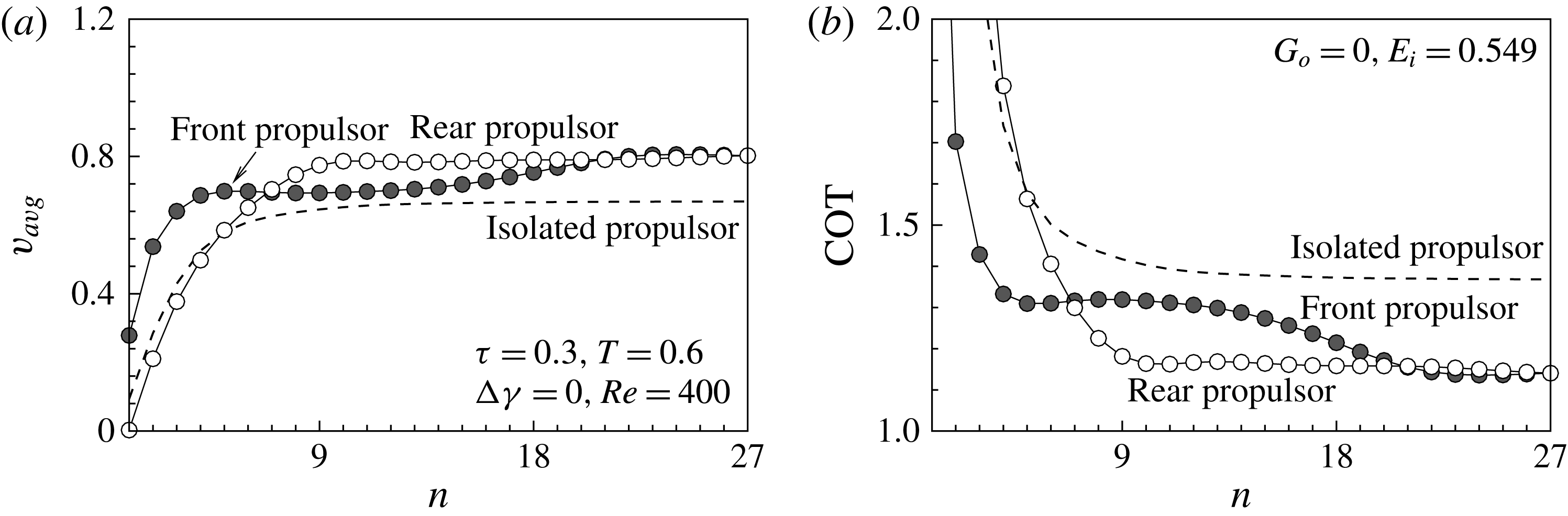
Figure 7(a,b) show the average velocity and the cost of transport during the $n$ th flapping period. During the initial flapping periods, the average velocity of FP exceeded that of IP, whereas the velocity of RP was lower than that of IP. As FP and RP formed a stable configuration, the average velocity converged to 0.8, larger than the value of IP. In figure 7(b), the cost of transport (COT), defined by the energy required to travel a unit distance during one flapping period, is expressed as

(3.1)

$$\begin{eqnarray}\text{COT}=f\,E_{i}/v_{avg},\end{eqnarray}$$

where $f$ is the flapping frequency and $E_{i}$ stands for the energy required to contract the bell during one flapping period. The energy required for the flapping behaviour is defined as the work done by the driving force to deform the body. In the present study, the driving force is the body force $F_{b}$ . The energy is a function of the body force and the bell deformation as expressed by

(3.2)

$$\begin{eqnarray}E_{i}=\int _{t_{0}}^{t_{0}+T}F_{b}\frac{\text{d}r}{\text{d}t}\,\text{d}t,\end{eqnarray}$$

where $\text{d}r/\text{d}t$ is the rate of change in the bell diameter. The bell deformation is mainly affected by $F_{b}$ . Many biological propulsors in nature exploit energy by fluid environments and reduce their cost of locomotion. For different fluid environments, they modulate their flapping behaviours as a way of reducing energy use. We focused on the flapping behaviours derived by the same driving forces for both FP and RP, in lieu of considering the modulation of flapping behaviours for different fluid environments. The dashed lines in figure 7 indicate the centre velocity and COT for IP, indicating that propulsion in a tandem configuration is more favourable than propulsion in an isolated system, in terms of the locomotion velocity and cost.

Figure 7.

(a) The average centre velocity, (b) the cost of transport, measured during the $n$ th flapping period. The symbols indicate the simulation of two tandem swimming propulsors with different initial positions, and the dashed line indicates an isolated swimming propulsors.

3.3 Flow-mediated interaction between propulsors

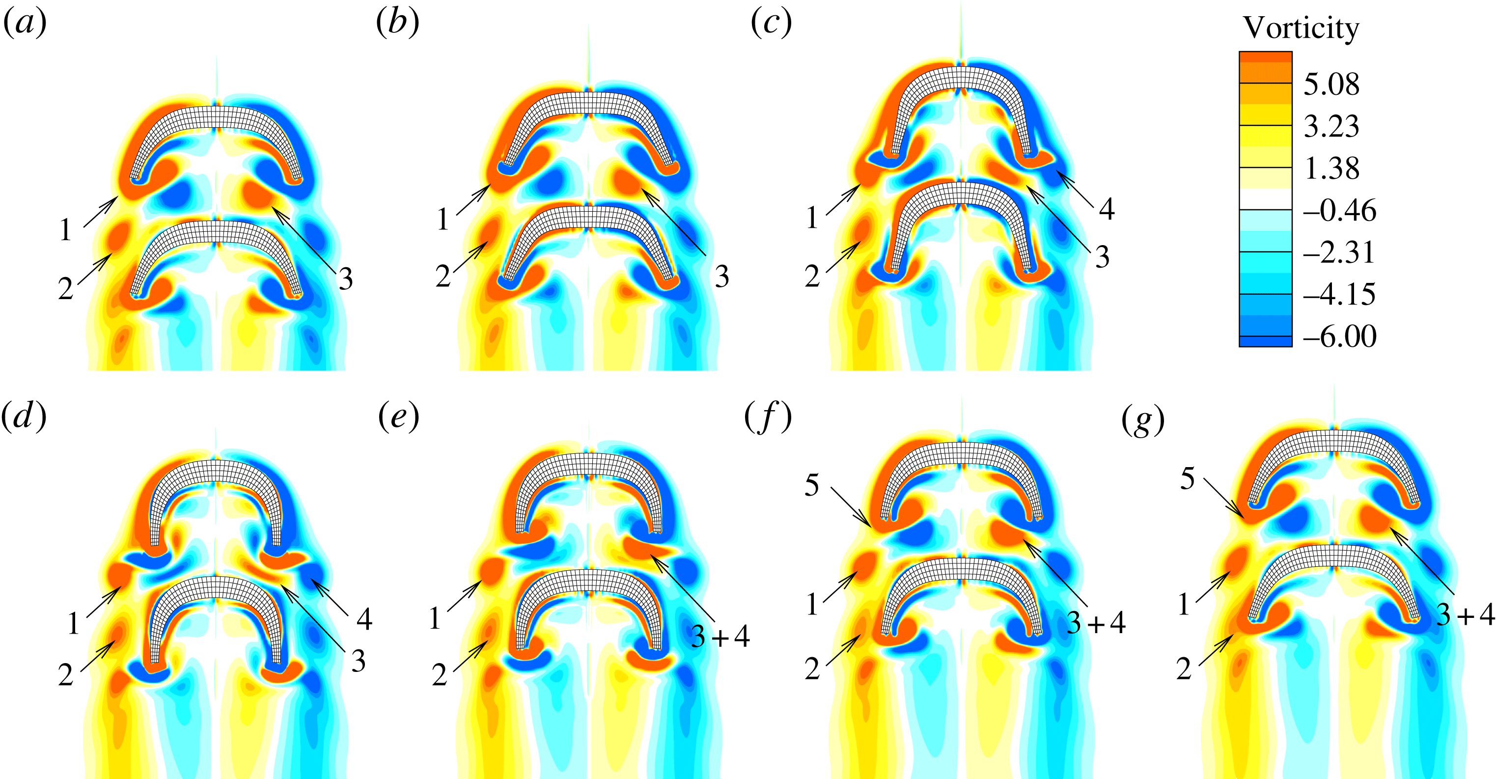
Different initial gap distances yielded the same stable configuration. Figure 8 visualizes the vortical structures generated during the 20th flapping period as FP and RP created propulsion in the stable configuration. For a given phase in the flapping frequency, the vortical structures generated in the wake may be denoted by numbers. The structures denoted by 1 correspond to the stopping vortex structures generated during the previous relaxation period, i.e. the 19th flapping period. The structures denoted by 2 are also stopping vortex structures but are generated during the 18th flapping period and shed from the tip. The structures indicated by 3 are the starting vortex structures generated during the previous contraction period. As in figure 8(a), the vortical structures generated during the previous strokes surround both FP and RP and interact with one another through complicated mechanisms by which both flexible propulsors may obtain hydrodynamic advantages. The structures 1 generated during the previous relaxation period are shed from the bell tip during the present contraction phase, as shown in figure 8(b–d). Figure 8(c) shows that the structure denoted by 4 is the staring vortex structure generated by the present power stroke and merges into structure 3. As the relaxation period proceeds, the stopping vortical structures denoted by 5 are generated near the bell tip, as shown in figure 8(e–g).

Figure 8.

Vortical structures in the wake during the 20th flapping period. (a) $t/T=20$ , (b) $t/T=20+1/6$ , (c) $t/T=20+2/6$ , (d) $t/T=20+3/6$ , (e) $t/T=20+4/6$ , (f) $t/T=20+5/6$ , (g) $t/T=21$ . The phase difference in the flapping frequency is ${\rm\Delta}{\it\gamma}={\rm\pi}$ . The vortical structures generated are denoted by the following numbers. 1: stopping vortical structures generated during the 19th flapping period; 2: stopping vortical structures generated during the 18th flapping period; $3+4$ : merging of the starting vortical structures produced during the previous and present power stroke; 5: stopping vortical structures generated by the present recovery stroke.

Figure 9.

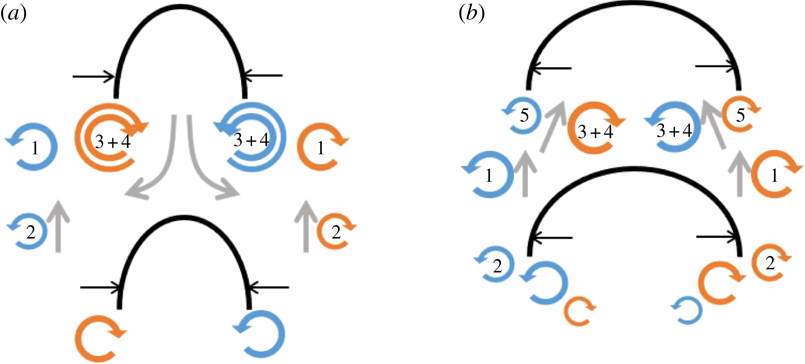
Schematic diagram showing the vortical structures during (a) the power stroke and (b) the recovery stroke. The numbers indicating the generated vortical structures are the same as those used in figure 8. The arrows indicate the directions of the fluid motions induced by the vortical structures.

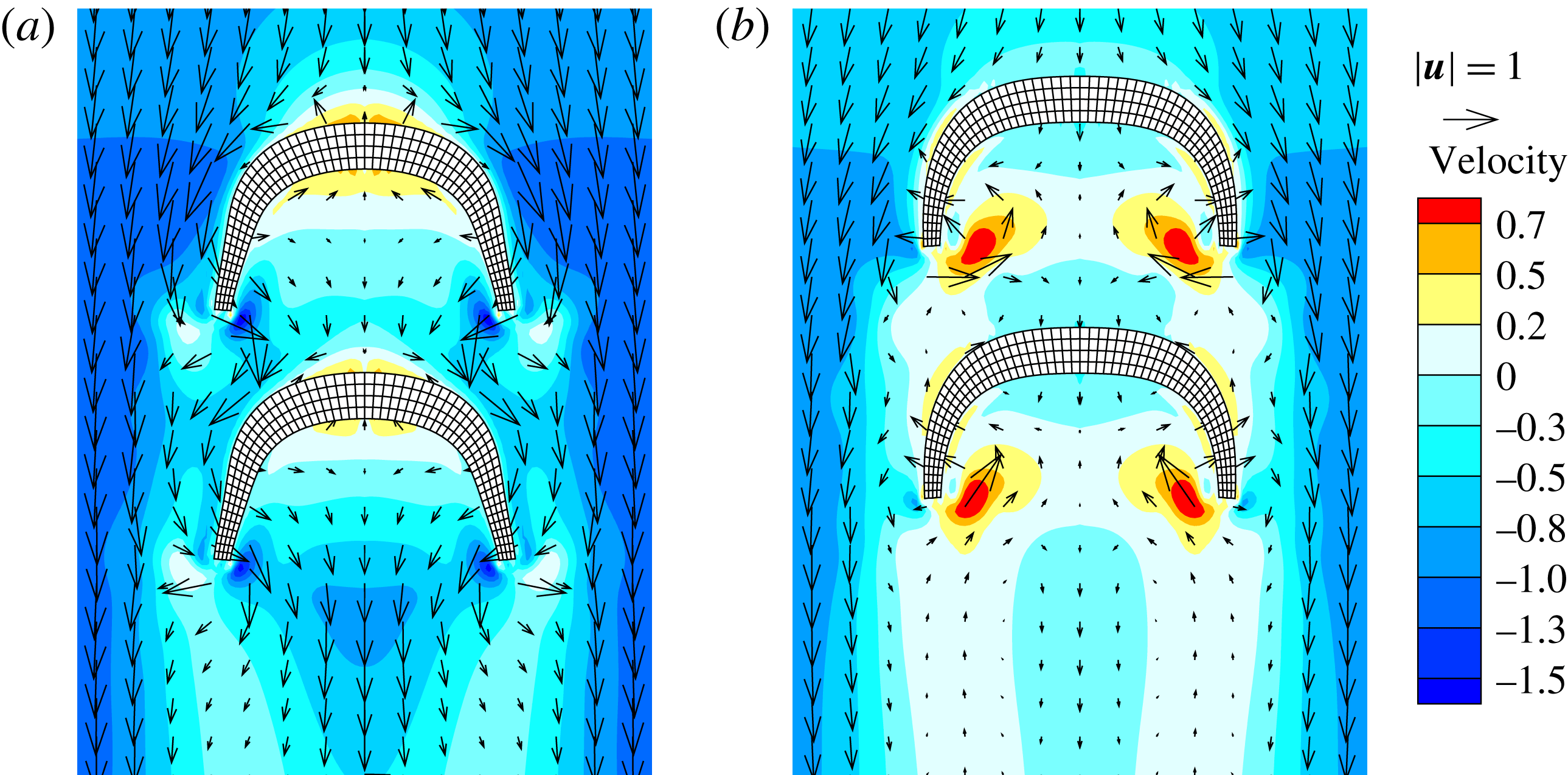
Figure 9(a,b) show a schematic diagram of the vortical structures and the induced fluid motions during the contraction and relaxation phase, respectively. As shown in figure 9(a), the merged starting vortex structures $(3+4)$ generated by the present and previous power strokes induced downward fluid motions that increased the drag on RP. Figure 9(b) shows that the surrounding fluid is injected into the bell during the relaxation period, and the vortical structures generated between FP and RP induce the fluid upward, reducing the resistance on RP. The fluid motions induced by the vortex–vortex interactions increased the distance between FP and RP during the contraction phase and decreased the distance during the relaxation phase in a stable configuration, as shown in figure 6. Figure 10 shows that the fluid motions could be visualized based on the velocity vectors and contours, indicating the velocity relative to the centre velocity (RP) in the $y$ direction. During the contraction phase, the flow was induced downward and shed along the bell of the RP, as shown in figure 10(a). During the recovery stroke, the surrounding fluid is injected into the inside near the bell tip, induced by the vortical structures 5 and $3+4$ , as shown in figures 9(b) and 10(b). Figure 10(b) shows that the downward momentum in the upstream of RP is less than the momentum in the upstream of FP due to the stopping vortex (denoted by 1) shed from FP.

Figure 10.

Flow velocity vector fields surrounding two tandem swimming propulsors during the 20th flapping period. (a) $t/T=20+2/6$ , (b) $t/T=20+4/6$ . The flow velocity in the $y$ direction is relative to the centre velocity of RP. The contour indicates the magnitude of the velocity.

3.4 Effects of the phase difference in the flapping frequencies on propulsion

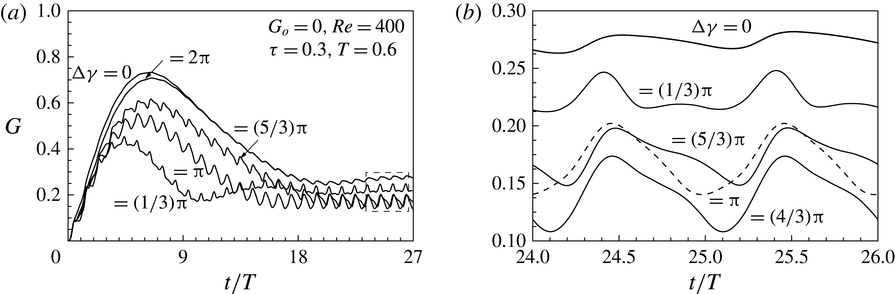
The initial gap distance between the FP and RP did not significantly influence the stable configuration, although the phase difference in the flapping frequency between FP and RP did affect the propulsion. Figure 11(a,b) show the gap distances between FP and RP for different phase differences in the flapping frequency. The initial gap distance was set to zero. Figure 11(b) shows the gap distances during the 24th and 25th flapping periods for different $y$ -scales. During the beginning of the propulsion, the FP flapped earlier than the RP when separated by a phase difference, as in (2.9). RP initiated the power stroke just as FP finished the recovery stroke for ${\rm\Delta}{\it\gamma}={\rm\pi}$ . When the phase difference is set to $2{\rm\pi}$ , FP and RP flap in-phase and reach the stable configuration found at ${\rm\Delta}{\it\gamma}=0$ , as shown in figure 10(a). 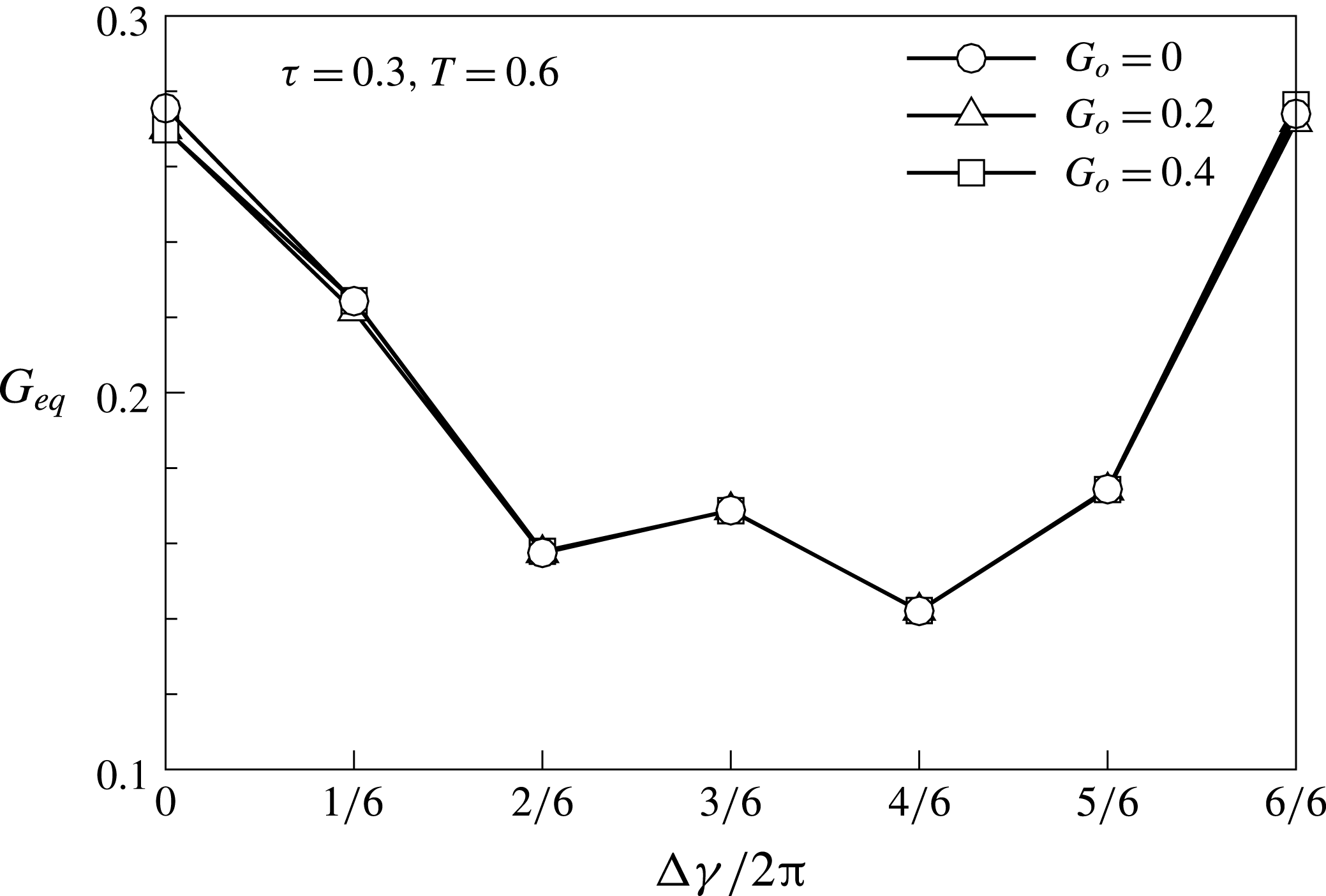The phase difference in the flapping frequency reduced the time required to reach a stable configuration, compared with the in-phase case $({\rm\Delta}{\it\gamma}=0)$ , and enabled the system to reach the characteristic gap distance of the stable configuration. As shown in figure 11(b), from the view point of FP, the gap distance between FP and RP increased during the contraction period and decreased during the relaxation period, thereby maintaining each stable configuration. The increasing and decreasing trends in the gap distance differed from the phase difference in the flapping frequency. A phase difference in the flapping frequency affected the mechanisms underlying the flow-mediated interactions between FP and RP, thereby inducing differences in the amplitude of the gap distance oscillation. The different initial gap distances and the average equilibrium position are plotted as a function of the phase difference in the flapping frequency, as shown in figure 12. Figure 12 shows that the stable configuration is affected by the phase difference in the flapping frequency and not by the initial gap distance. The in-phase system $({\rm\Delta}{\it\gamma}=0,2{\rm\pi})$ was characterized by a gap distance that exceeded the gap distance found in other out-of-phase cases. As the amplitude in the gap distance oscillation increased, the equilibrium gap distance generally decreased, as shown in figures 11(b) and 12. The generated vortical structures and stable configurations of FP and RP are shown in the supplementary movie 1 available at http://dx.doi.org/10.1017/jfm.2016.148.

Figure 11.

Time histories of the gap distance between two tandem propulsors, given different phase differences in the flapping frequency. (a) $0<t/T<27$ ; $G_{o}=0$ , $Re=400$ , ${\it\tau}=0.3$ , $T=0.6$ and (b) enlarged view, $24<t/T<26$ .

Figure 12.

The equilibrium gap distance $G_{eq}$ as a function of the phase difference in the flapping frequency.

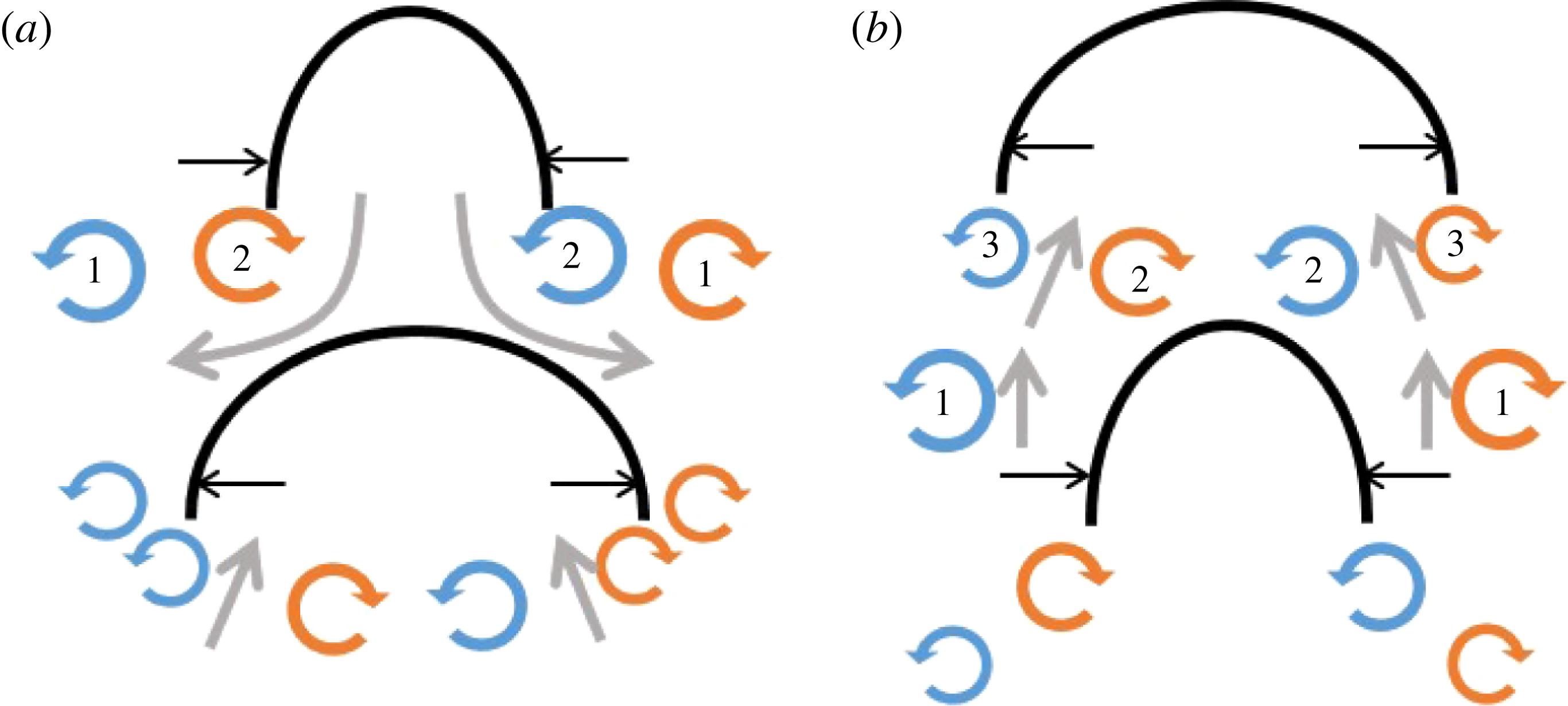
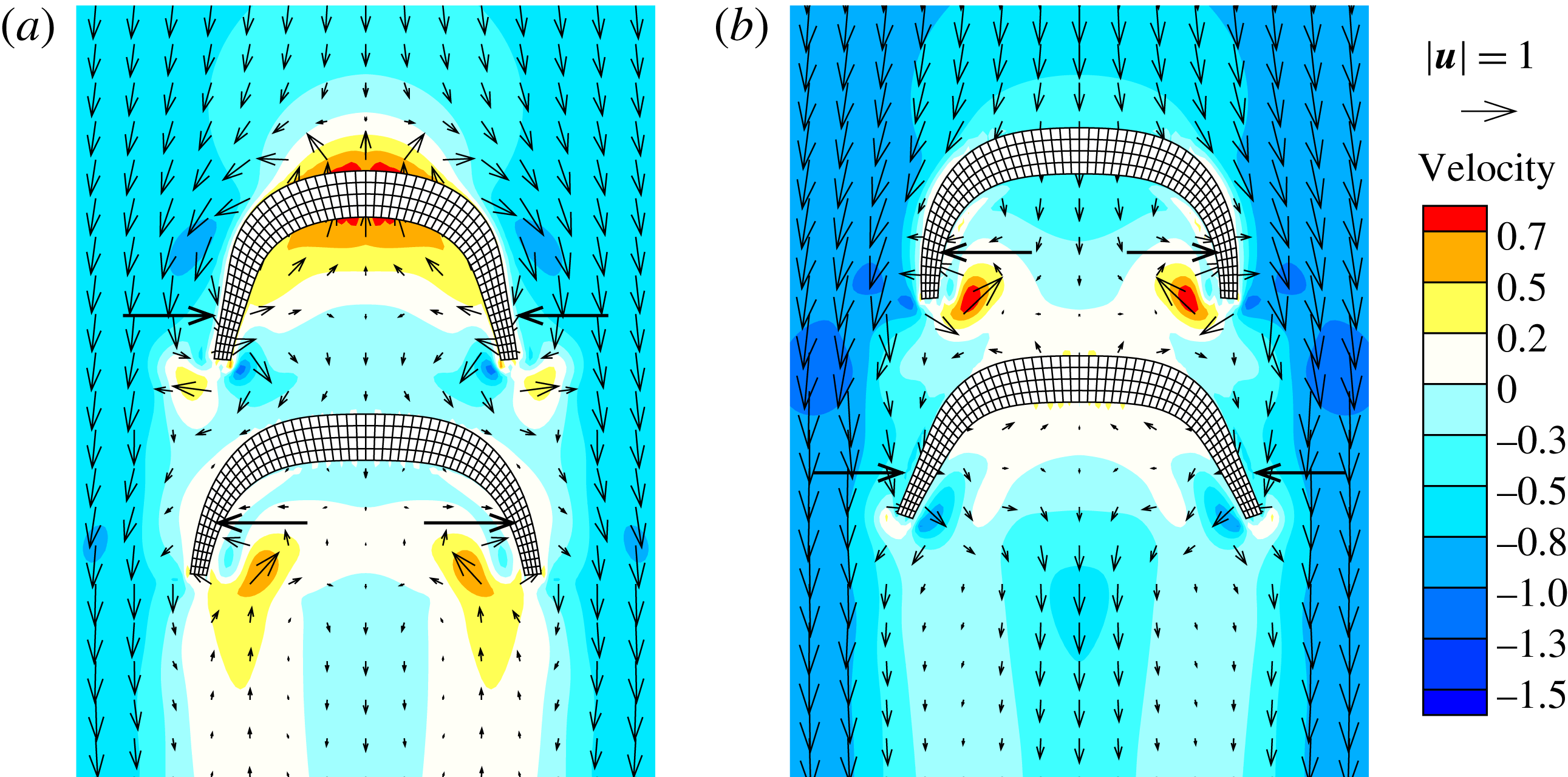
Figure 13 shows a schematic diagram of the vorticity structures generated by FP and RP for ${\rm\Delta}{\it\gamma}={\rm\pi}$ . During the contraction phase of FP, the stopping vortex structures produced during the previous recovery stroke are denoted by 1 and are shed from the tip, as shown in figure 13(a). The starting vortical structures denoted by 2 are generated and induce a downward transport of the surrounding fluid, indicating a thrust wake. In the system characterized by out-of-phase flapping frequencies, the surrounding fluid induced by FP encounters RP as the bell reaches an extended state, thereby generating a lateral wake that is larger than the wake formed in the in-phase case, as shown in figures 9(a) and 13(a). Figure 13(b) shows that during the relaxation phase of the FP, the surrounding fluid motions induced by the generated vortical structures favour propulsion of RP, reducing the resistance on RP. The mechanisms underlying the flow-mediated interactions explained the increasing and decreasing trends in the gap distances during the contraction and relaxation phases of FP, respectively. Figure 14 shows the $y$ -direction velocity contours, which indicated the magnitudes of the velocities relative to the centre velocity of the RP for ${\rm\Delta}{\it\gamma}={\rm\pi}$ . The lateral wakes present between the FP and RP are shown in the velocity vector field in figure 14(a). Figure 14(b) shows that the fluid between the FP and RP flow into the FP bell and favour RP locomotion, reducing the gap distance between them during the relaxation period of FP.

Figure 13.

Schematic diagram showing the vortical structures during (a) the power stroke and (b) the recovery stroke, from the viewpoint of FP. The vortical structures generated are denoted by the following numbers. 1: stopping vortical structures generated during the previous flapping period; 2: starting vortical structures generated by the present power stroke; 3: stopping vortical structures generated by the present recovery stroke. The arrows indicate the directions of the fluid motions induced by the vortical structures. The phase difference in the flapping frequencies is ${\rm\Delta}{\it\gamma}={\rm\pi}$ .

Figure 14.

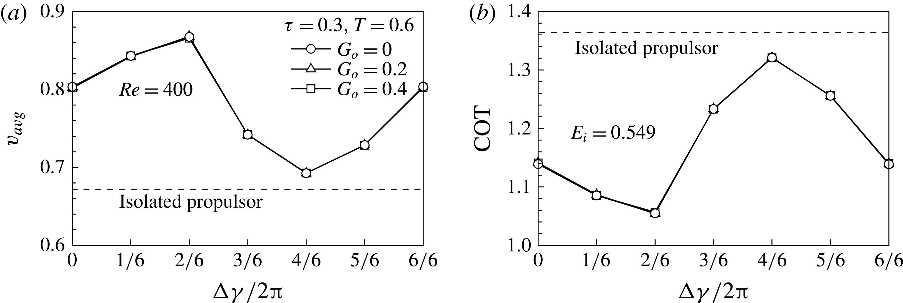
Figure 15 shows the centre velocity and the cost of transport given different phase differences in the flapping frequency. The centre velocity and the transport cost depend on the phase difference in the flapping frequency, not the initial gap distance. For tandem flexible propulsors with a paddling-based locomotion, as shown in figure 15(a) and the supplementary movie 1, the centre velocity has an optimal value as the flapping frequency phase difference between FP and RP is set to $(2/3){\rm\pi}$ , where they move 29 % faster than IP. The minimum value of the average velocity of the propulsion in a tandem configuration, measured for ${\rm\Delta}{\it\gamma}=(4/3){\rm\pi}$ , exceeded the propulsion velocity of IP. The cost of transport for FP and RP is lower than that of IP, implying that the propulsors in a tandem configuration can move farther than IP for a given input power.

Figure 15.

(a) The centre velocity and (b) the cost of transport as a function of the phase difference in the flapping frequency. The dashed line indicates the centre velocity and the cost of transport of the isolated propulsor.

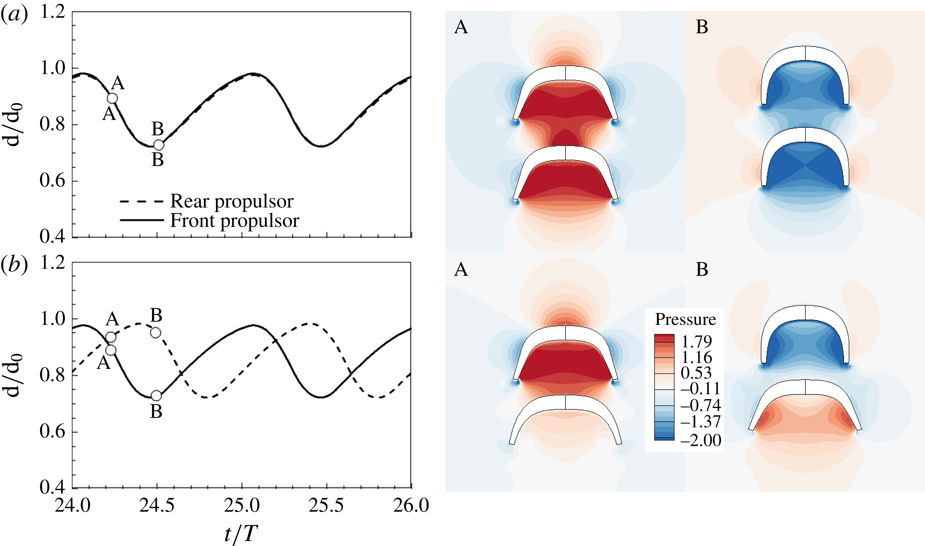
Both FP and RP benefited from the tandem propulsion formations and the hydrodynamic interactions were affected by the phase difference in the flapping frequency. Figure 16 shows the time histories of the normalized diameter and the pressure contours for ${\rm\Delta}{\it\gamma}=0$ and $2{\rm\pi}/3$ . The flapping behaviours of FP and RP are the same when the phase difference is zero. During the contraction phase, FP was benefited from the tandem formation. As the contraction proceeded, the pressure inside the bells of FP and RP increased (a-A). As compared to the pressure in the downstream of IP in figure 4(b), the pressure in the downstream of FP increased due to RP, leading to the beneficial effects on the propulsion of FP during the contraction phase. RP was benefited during the relaxation phase since the pressure in the upstream of RP decreased, reducing the pressure gradient across the bell of RP. From the hydrodynamic point of view, unlike the case where the phase difference was zero, both FP and RP were benefited during the contraction phase when the phase difference was $2{\rm\pi}/3$ . At point A in figure 16(b), FP and RP are in the midst of the contraction and relaxation phases, respectively. In terms of FP, during the contraction phase, the increased pressure in the downstream of FP due to the existence of RP was beneficial for the propulsion of FP. During the contraction phase of RP (B), RP was benefited from the tandem formation by the decreased pressure in the upstream of RP. Two tandem paddling propulsors showed an optimal propulsion in terms of the centre velocity and the locomotion cost when the phase difference was $(2/3){\rm\pi}$ where both FP and RP were benefited during the contraction phase from the viewpoint of the hydrodynamic pressure.

Figure 16.

Time histories of the normalized diameter for (a) ${\rm\Delta}{\it\gamma}=$ 0 and (b) ${\rm\Delta}{\it\gamma}=2{\rm\pi}/3$ . The pressure contours for (a) ${\rm\Delta}{\it\gamma}=0$ and (b) ${\rm\Delta}{\it\gamma}=2{\rm\pi}/3$ are shown at A $(t/T=24+2/6)$ and B $(t/T=24+3/6)$ . The contour level for pressure is the same as in figure 4.

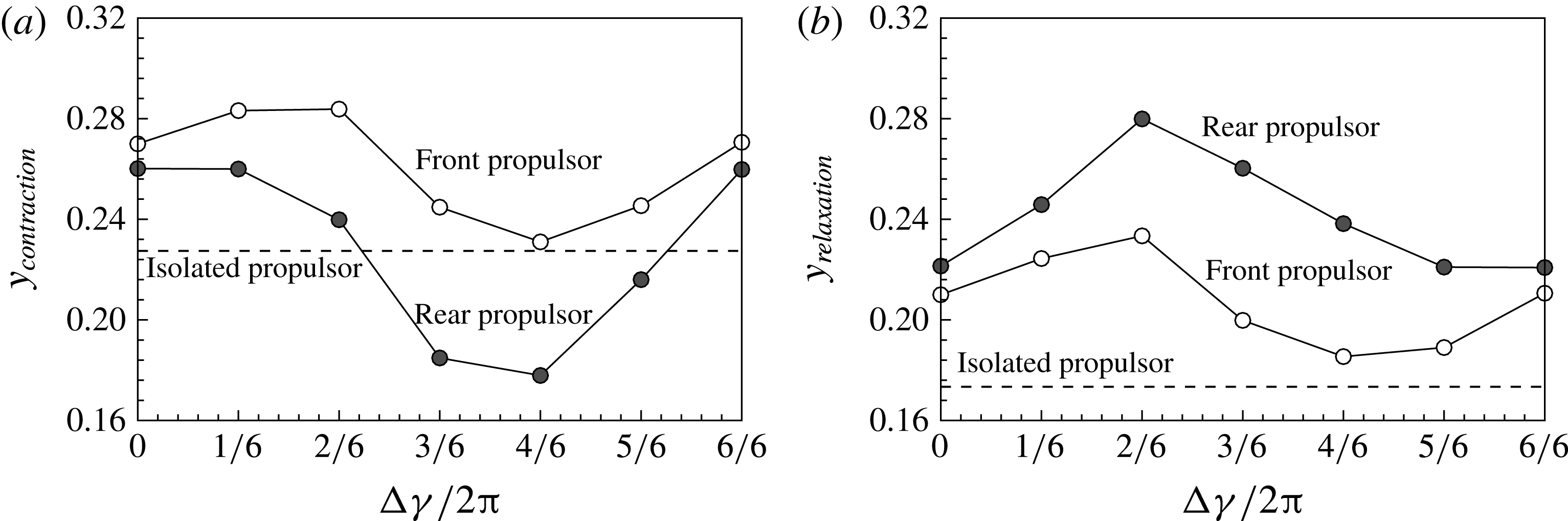
Figure 17 shows the moving distances of FP and RP during the contraction $(24<t/T<24.5)$ and relaxation $(24.5<t/T<25)$ phases of FP. As shown in figure 17(a,b), FP benefited not only during the contraction phase, but also during the relaxation phase. RP is faster than FP during the relaxation phase of FP, increasing the favourable flow velocity in the wake of FP (figure 14 b). Daghooghi & Borazjani (Reference Daghooghi and Borazjani2015) addressed the hydrodynamic advantage of synchronized swimming fish in a rectangular pattern where they moved up to 20 % faster than a solitary swimmer. The hydrodynamic advantage from the rectangular pattern was originated from the enhanced flow between the swimmers in the direction of swimming, which is called the channelling effect. This is analogous to the present tandem swimmers with a paddling-based locomotion. FP in the midst of the relaxation phase benefited from the enhanced flow in the direction of swimming. The favourable flow in the wake of FP imparted momentum to FP in the moving direction, which helped FP swim faster than IP. During the relaxation phase of FP, RP benefited from the decreased hydrodynamic pressure in the upstream of RP as compared to the pressure in the upstream of IP. However, during the contraction phase, RP was penalized due to the increased hydrodynamic pressure in the wake of FP. Accordingly, RP moved slower than FP and even than IP for some phase differences in figure 17(a). Figure 17(b), on the other hand, shows that RP moved farther than FP and IP during the relaxation phase of FP, implying that the penalty experienced by RP could be compensated by swimming in the wake of FP (figure 4 e).

Figure 17.

The moving distances of FP and RP during the (a) contraction $(24<t/T<24.5)$ and (b) relaxation $(24.5<t/T<25)$ phases of FP.

Recall in figure 7(a) that FP moved much faster than RP and IP during the initial flapping periods since FP benefited from the tandem formation, while RP was penalized during the contraction phase of FP. As the moving velocity of FP increased, the benefit experienced by FP was reduced, leading to a local plateau in the FP velocity (5th–8th flapping periods). The flow velocity in the wake of FP increased in the moving direction as the moving velocity of FP increased, which helped the locomotion of RP in the wake of FP. As a result, RP moved faster than IP and FP after the seventh flapping period. The gap distance between FP and RP decreased and FP benefited from the tandem formation, increasing the propulsion velocity of FP again. Finally, they reached a stable configuration and moved farther than that of IP for the same power input.

In this section, we have discussed vortex–vortex and vortex–body interactions of a tandem flexible propulsor with a paddling-based locomotion and their dependence on the initial gap distance and the phase difference in the flapping frequency. Stable configurations and energetic advantages were obtained in two tandem paddling propulsors as observed in the numerical study of self-propelled tandem flags (Zhu et al. Reference Zhu, He and Zhang2014). The hydrodynamic interactions described in the present study would be valid for a pair of tandem oblate propulsors with a paddling-based locomotion if the flapping frequency is constant and equal to each other. However, as the Reynolds number increased, a stable configuration was not obtained since the vorticity generated from FP dissipated before interacting with RP (not shown here). The hydrodynamic interactions could also be affected by the propulsor shape. A simulation was performed for the prolate flexible propulsor (not shown), where jet structures were observed in the wake rather than wide vortical structures near the bell margin observed in the oblate flexible propulsor. In the wake of the prolate flexible propulsor with a jet-based locomotion, the starting vortical structures generated during the contraction phase were shed downstream instead of remaining near the bell margin and interacting with the stopping vortical structures, and a stable configuration was not obtained.

4 Conclusions

The present study investigated the dynamics of two tandem self-propelled propulsors with a paddling-based locomotion using the immersed boundary method. After a few initial flapping periods, FP and RP formed a stable configuration spontaneously, in which the gap distance increased and decreased during the contraction and relaxation phases of FP. A constant phase difference in the flapping frequencies of the propulsors produced the same stable configuration, regardless of the initial gap distance, although the time required to reach the stable configuration depended on this distance. The stable configuration was largely affected by the phase difference in the flapping frequency because the flow-mediated interaction mechanisms depended on the phase difference. An optimal propulsion was obtained when the phase difference was $(2/3){\rm\pi}$ where both FP and RP benefited during the contraction phase. Both flexible propulsors in a tandem configuration enjoyed locomotion velocity and cost benefits from the coupled propulsion compared to an isolated propulsion system. Investigations of the mechanisms by which flow-mediated interactions are processed between flexible propulsors in a tandem configuration suggest a foundational mechanism by which swimmers may gain benefits from schooling behaviours.

Acknowledgements

This study was supported by the Creative Research Initiatives (no. 2016-004749) program of the National Research Foundation of Korea (MSIP).

Supplementary movie

A supplementary movie is available online at http://dx.doi.org/10.1017/jfm.2016.148.

References

Alben, S. 2009 Wake-mediated synchronization and drafting in coupled flags. J. Fluid Mech. 641, 489–496.Google Scholar

Alben, S. & Shelley, M. 2005 Coherent locomotion as an attracting state for a free flapping body. Proc. Natl Acad. Sci. USA 102, 11163–11166.Google Scholar

Beal, D. N., Hover, F. S., Triantafyllou, M. S., Liao, J. C. & Lauder, G. V. 2006 Passive propulsion in vortex wakes. J. Fluid Mech. 549, 385–402.Google Scholar

Belyayev, V. V. & Zuyev, G. V. 1969 Hydrodynamic hypothesis of schooling in fish. J. Ichthy 9, 578–584.Google Scholar

Borazjani, I. 2015 Simulations of unsteady aquatic locomotion: from unsteadiness in straight-line swimming to fast-starts. Integr. Compar. Biol. 55, 740–752.Google Scholar

Breder, C. M. Jr 1976 Fish schools as operational structures. Fish. Bull. 74, 471–502.Google Scholar

Colin, S. P. & Costello, J. H. 2002 Morphology, swimming performance and propulsive mode of six co-occurring hydromedusae. J. Expl Biol. 2002, 427–437.Google Scholar

Dabiri, J. O. 2005 On the estimation of swimming and flying forces from wake measurements. J. Expl Biol. 208, 3519–3532.CrossRef Google Scholar PubMed

Dabiri, J. O. 2009 Optimal vortex formation as a unifying principle in biological propulsion. Annu. Rev. Fluid Mech. 41, 17–33.CrossRef Google Scholar

Dabiri, J. O., Colin, S. P., Costello, J. H. & Gharib, M. 2005 Flow patterns generated by oblate medusa jellyfish: field measurements and laboratory analyses. J. Expl Biol. 208, 1257–1265.Google Scholar

Daghooghi, M. & Borazjani, I. 2015 The hydrodynamic advantages of synchronized swimming in a rectangular pattern. Bioinspir. Biomim. 10, 056018.Google Scholar

Eldredge, J. D. & Pisani, D. 2008 Passive locomotion of a simple articulated fish-like system in the wake of an obstacle. J. Fluid Mech. 607, 279–288.Google Scholar

Fish, F. E. & Lauder, G. V. 2006 Passive and active flow control by swimming fishes and mammals. Annu. Rev. Fluid Mech. 38, 193–224.CrossRef Google Scholar

Gemmell, B. J., Costello, J. H., Colin, S. P., Stewart, C. J., Dabiri, J. O., Tafti, D. & Priya, S. 2013 Passive energy recapture in jellyfish contributes to propulsive advantage over other metazoans. Proc. Natl Acad. Sci. USA 110, 17904–17909.Google Scholar

Graham, W. M., Pages, F. & Hamner, W. M. 2001 A physical context for gelatinous zooplankton aggregations: a review. Hydrobiologia 451, 199–212.Google Scholar

Huang, W.-X. & Sung, H. J. 2009 An immersed boundary method for fluid–flexible structure interaction. Comput. Meth. Appl. Mech. Engng 198, 2650–2661.Google Scholar

Jang, S. J., Sung, H. J. & Krogstad, P. 2011 Effects of an axisymmetric contraction on a turbulent pipe flow. J. Fluid Mech. 687, 376–403.Google Scholar

Kim, K., Baek, S. J. & Sung, H. J. 2002 An implicit velocity decoupling procedure for incompressible Navier–Stokes equations. Intl J. Numer. Meth. Fluids 38, 125–138.Google Scholar

Kim, S., Huang, W.-X. & Sung, H. J. 2010 Constructive and destructive interaction modes between two tandem flexible flags in viscous flow. J. Fluid Mech. 661, 511–521.Google Scholar

Lauder, G. V. & Jayne, B. C. 1996 Pectoral fin locomotion in fishes: testing drag-based models using three-dimensional kinematics. Am. Zool. 36, 567–581.Google Scholar

Liao, J. C., Beal, D. N., Lauder, G. V. & Triantafyllou, M. S. 2003a Fish exploiting vortices decrease muscle activity. Science 302, 1566–1569.Google Scholar

Liao, J. C., Beal, D. N., Lauder, G. V. & Triantafyllou, M. S. 2003b The Karman gait: novel body kinematics of rainbow trout swimming in a vortex street. J. Expl Biol. 206, 1059–1073.Google Scholar

Linden, P. F. & Turner, J. S. 2004 ‘Optimal’ vortex rings and aquatic propulsion mechanisms. Proc. R. Soc. Lond. B 271, 647–653.Google Scholar

Mchenry, M. J. & Jed, J. 2003 The ontogenetic scaling of hydrodynamics and swimming performance in jellyfish (Aurelia aurita). J. Expl Biol. 206, 4125–4137.Google Scholar

Megill, W. M.2002 The biomechanics of jellyfish swimming. PhD thesis, The University of British Columbia.Google Scholar

Muller, U. K., van den Heuvel, B. L. E., Stamhuis, E. J. & Videler, J. J. 1997 Fish foot prints: morphology and energetics of the wake behind a continuously swimming mullet (Chelon labrosus Risso). J. Expl Biol. 200, 2893–2906.CrossRef Google Scholar

Park, S. G., Chang, C. B., Huang, W. H. & Sung, H. J. 2014 Simulation of swimming oblate jellyfish with a paddling-based locomotion. J. Fluid Mech. 748, 731–755.CrossRef Google Scholar

Ristroph, L. & Zhang, J. 2008 Anomalous hydrodynamic drafting of interacting flapping flags. Phys. Rev. Lett. 101, 194502.Google Scholar

Rottini Sandrini, L., Stravisi, J. & Pieri, G. 1980 A recent shift in the wind distribution and the appearance of unusual planktonic organisms in the Gulf of Trieste. Boll. Soc. Adr. Sci Trieste 64, 77–84.Google Scholar

Sahin, M. & Mohseni, K. 2009 An arbitrary Lagrangian–Eulerian formulation for the numerical simulation of flow patterns generated by the hydromedusa Aequorea victoria . J. Comput. Phys. 228, 4588–4605.Google Scholar

Sahin, M., Mohseni, K. & Colin, S. P. 2009 The numerical comparison of flow patterns and propulsive performances for the hydromedusae Sarsia tubulosa and Aequorea victoria . J. Expl Biol. 212, 2656–2667.Google Scholar

Shin, S. J., Huang, W.-X. & Sung, H. J. 2008 Assessment of regularized delta functions and feedback forcing schemes for an immersed boundary method. Intl J. Numer. Meth. Fluids 58, 263–286.CrossRef Google Scholar

Tytell, E. D. & Lauder, G. V. 2004 The hydrodynamics of eel swimming. I. Wake structure. J. Expl Biol. 207, 1825–1841.Google Scholar

Uddin, E., Huang, W.-X. & Sung, H. J. 2013 Interaction modes of multiple flexible flags in a uniform flow. J. Fluid Mech. 729, 563–583.Google Scholar

Ulrike, K. M. 2003 Fish ’n flag. Science 302, 1511–1512.Google Scholar

Weihs, D. 1973 Hydromechanics of fish schooling. Nature 241, 290–291.Google Scholar

Zavodnik, D. 1987 Spatial aggregations of the swarming jellyfish Pelagia noctiluca (Scyphozoa). Mar. Biol. 94, 265–269.Google Scholar

Zhang, J., Childress, S., Libchaber, A. & Shelley, M. 2000 Flexible filaments in a flowing soap film as a model for one-dimensional flags in a two-dimensional wind. Nature 408, 835–839.Google Scholar

Zhao, H., Freund, J. B. & Moser, R. D. 2008 A fixed-mesh method for incompressible fluid–structure systems with finite solid deformations. J. Comput. Phys. 227, 3114–3140.CrossRef Google Scholar

Zhu, X., He, G. & Zhang, X. 2014 Flow-mediated interactions between two self-propelled flapping filaments in tandem configuration. Phys. Rev. Lett. 113, 238105.Google Scholar

Figure 1.(a) Schematic diagram of two tandem swimming propulsors in a quiescent fluid and in a cylindrical computational domain. (b) Schematic diagram showing the propulsor bell, including the grid and the body force applied to the bell. Point 1 is on the centre axis and has the same $y$ location as point 3. Point 2 denotes the bell tip. Point 3 is the forcing point which satisfies the condition of the body force range in (2.9): ${\it\tau}=0.3$, $T=0.6$, ${\it\phi}=300$. (c) The time histories of the body force. The solid and dashed lines denote the body forces on the front and rear propulsors, respectively.

Table 1.Physical and numerical parameters.

Figure 2.Time histories of (a) the fineness ratio and (b) the centre velocity.

Figure 3.Time histories of the centre velocities over the different domain sizes (a), for different numbers of grids in the longitudinal and radial directions (b), and for different numbers of grid in the azimuthal direction (c).

Figure 4.Time histories of (a) the normalized diameter and (b) the centre position in the moving direction and the pressure contours at A $(t/T=8)$, B $(t/T=8+2/6)$, C $(t/T=8+3/6)$ and D $(t/T=8+4.5/6)$. Velocity contour in the moving direction at E $(t/T=8+2/6)$.

Figure 5.Time histories of the centre velocity. (a) $G_{o}=0$, $Re=400$, (b) $G_{o}=6$.

Figure 6.Time histories of the gap distance between the tandem propulsors for different initial positions.

Figure 7.(a) The average centre velocity, (b) the cost of transport, measured during the $n$th flapping period. The symbols indicate the simulation of two tandem swimming propulsors with different initial positions, and the dashed line indicates an isolated swimming propulsors.

Figure 8.Vortical structures in the wake during the 20th flapping period. (a) $t/T=20$, (b) $t/T=20+1/6$, (c) $t/T=20+2/6$, (d) $t/T=20+3/6$, (e) $t/T=20+4/6$, (f) $t/T=20+5/6$, (g) $t/T=21$. The phase difference in the flapping frequency is${\rm\Delta}{\it\gamma}={\rm\pi}$. The vortical structures generated are denoted by the following numbers. 1: stopping vortical structures generated during the 19th flapping period; 2: stopping vortical structures generated during the 18th flapping period; $3+4$: merging of the starting vortical structures produced during the previous and present power stroke; 5: stopping vortical structures generated by the present recovery stroke.

Figure 9.Schematic diagram showing the vortical structures during (a) the power stroke and (b) the recovery stroke. The numbers indicating the generated vortical structures are the same as those used in figure 8. The arrows indicate the directions of the fluid motions induced by the vortical structures.

Figure 10.Flow velocity vector fields surrounding two tandem swimming propulsors during the 20th flapping period. (a) $t/T=20+2/6$, (b) $t/T=20+4/6$. The flow velocity in the $y$ direction is relative to the centre velocity of RP. The contour indicates the magnitude of the velocity.

Figure 11.Time histories of the gap distance between two tandem propulsors, given different phase differences in the flapping frequency. (a) $0; $G_{o}=0$, $Re=400$, ${\it\tau}=0.3$, $T=0.6$ and (b) enlarged view, $24.

Figure 12.The equilibrium gap distance $G_{eq}$ as a function of the phase difference in the flapping frequency.

Figure 13.Schematic diagram showing the vortical structures during (a) the power stroke and (b) the recovery stroke, from the viewpoint of FP. The vortical structures generated are denoted by the following numbers. 1: stopping vortical structures generated during the previous flapping period; 2: starting vortical structures generated by the present power stroke; 3: stopping vortical structures generated by the present recovery stroke. The arrows indicate the directions of the fluid motions induced by the vortical structures. The phase difference in the flapping frequencies is ${\rm\Delta}{\it\gamma}={\rm\pi}$.

Figure 14.Flow velocity vector fields surrounding two tandem swimming propulsors during the 20th flapping period. (a) $t/T=20+2/6$, (b) $t/T=20+4/6$. The flow velocity in the $y$ direction is relative to the centre velocity of RP. The contour indicates the magnitude of the velocity.

Figure 15.(a) The centre velocity and (b) the cost of transport as a function of the phase difference in the flapping frequency. The dashed line indicates the centre velocity and the cost of transport of the isolated propulsor.

Figure 16.Time histories of the normalized diameter for (a) ${\rm\Delta}{\it\gamma}=$ 0 and (b) ${\rm\Delta}{\it\gamma}=2{\rm\pi}/3$. The pressure contours for (a) ${\rm\Delta}{\it\gamma}=0$ and (b) ${\rm\Delta}{\it\gamma}=2{\rm\pi}/3$ are shown at A $(t/T=24+2/6)$ and B $(t/T=24+3/6)$. The contour level for pressure is the same as in figure 4.