


Why do Great Powers fight one another? This obviously central, and seemingly simple, question leads directly to one of the most frustrating gaps in the empirical literature on international conflict. Great Powers are states whose interests and capabilities extend beyond their immediate neighbors. More so than other states, they shape and respond to the structure of the international system. That structure is typically implicated in systemic wars, which evolve from the interactions of all of the major states in the system. Yet somehow, if the conflict literature is to be believed, those same states cease to be driven by systemic interests and systemic imperatives in the long stretches of time between systemic wars. In typical statistical models of conflict, they are pooled with all of the other states in the system, under the assumption that they respond in the same way to the same stimuli, which are typically both local and dyadic.Footnote 1 Because no one can predict with certainty whether a given crisis between Great Powers will be resolved without bloodshed or explode into a systemic war, however, arguing that only systemic wars have systemic causes is unsustainable.
The main barrier to understanding the systemic origins of Great Power conflict is that systemic theories of international politics are notoriously vague, in the sense that they are consistent with a wide range of possible state activities. Systemic theorists have been fairly open about this fact. Early efforts (e.g., Gulick Reference Gulick1955; Kaplan Reference Kaplan1957) developed explanations of the nature of the international system without attempting to derive or test hypotheses about state behavior; later systemic theorizing embraces the idea of prediction but typically only at the systemic level. Perhaps the clearest example of the latter is Mearsheimer (Reference Mearsheimer2001, 11), who distinguishes between high-level theories such as his own offensive realism and more fine-grained theories like deterrence theory, arguing that only the latter predict war. In those cases in which systemic theorists do predict war, they tend to focus on large-scale wars in which the governance of the international system is at issue rather than on interstate conflicts in general.Footnote 2
Rather than attempt to relate systemic characteristics directly to a general model of conflict, an effort that even the boldest systemic theorists have disavowed, or argue about whether a systemic theory can or should be a theory of foreign policy, this article combines theories from different levels of analysis in a two-step approach. First, it describes and tests an original systemic theory that explains the ongoing, dynamic interactions between the structure of the international system and the major states within it. Although their goals differ, the main actors in the system attempt to regulate its main features; because their goals differ, these attempts inevitably generate frictions between them. Next, it describes the process by which these frictions become militarized disputes and, in so doing, elaborates the circumstances under which they are most likely to do so. Although two competing models, the spiral model and the deterrence model, offer plausible answers to the latter question and the logic of the systemic model favors neither, the evidence favors the deterrence model.
Conjoining a new systemic theory of international relations with existing theories of conflict is an advance both for the conflict literature, which has been starved of systemic insights, and for the literature on systemic theory, which says little about conflict in general. Moreover, the test of the spiral versus the deterrence model in the second stage of the analysis is innovative and important in its own right. For decades the spiral model and the deterrence model have coexisted happily in the conflict literature, despite the fact that they contradict each other directly. Scholars are comfortable deriving theories of conflict that are implicitly based on one or the other, or arguing that some conflicts result from spirals whereas others result from failures of deterrence. Few works attempt to evaluate the predictions of the two models more generally, in order to assess which constitutes a better explanation of conflict. Moreover, because spiral-model examples are typically drawn from the period under study here, the conclusion that deterrence theory dominates the spiral model in a head-to-head test is a surprising one.
The article proceeds as follows. First, I describe the dynamics of Great Power interaction at the systemic level, both in general and in the context of the Vienna system, and show that the deterrence model and the spiral model constitute two ways of understanding how these interactions can produce conflict. Next, I describe the data used to test these arguments and the statistical models appropriate for doing so. I then present the results of the tests, illustrate them, and explore what the illustrations tell us about conflict processes. The final section concludes.
SYSTEMS, STATE ACTIVITY, AND CONFLICT
In this section, I argue that Great Power conflict can best be understood as the outcome of a two-step process. First, states engage in ongoing management of the structure of the international system by acting to alter the distributions of resources deemed relevant to security. States themselves decide which resources are relevant to security, often based on recent lessons of history: following the Napoleonic Wars, for example, Europeans saw threats to general stability in imbalances of power and in the spread of revolution from below, and they initially sought to prevent both. The actions necessary to manage the structure of the system create frictions between states, and in the second step, those frictions lead to dyadic conflict. The existing international relations literature offers two coherent but conflicting models that explain the timing of these dyadic conflicts: the spiral model, which suggests that self-reinforcing spirals of activity designed to prevent conflict will generate it instead; and the deterrence model, which suggests that high levels of security-related activity between states serve as mutual deterrents and that conflicts erupt when one state ignores the threat posed by another.
Systemic Politics
In systemic international relations theory, that which distinguishes the characteristics of individual states from the characteristics of the structure of the system is the distributional nature of the latter. Waltz (Reference Waltz1979, 98) makes this argument explicitly when arguing that the balance of power is an attribute of system structure. Buzan, Jones, and Little (Reference Buzan, Jones and Little1993, ch. 3) follow the same logic while questioning power's pride of place; and Wendt (Reference Wendt1999, ch. 3) bases his systemic theory on a different distribution entirely—the distribution of ideas.
Explaining the relationship between these distributions and the major actors in the system, however, is far from trivial. In Wendt's depiction, agents and “micro-structures” constitute one another, but neither determines macro-structural outcomes like distributions of power (1999, 48–50, 365–66). Waltz's structures “limit and mold agents and agencies and point them in ways that tend toward a common quality of outcomes even though the efforts and aims of agents and agencies vary” (1979, 74)—but agents play virtually no role, either in determining their own fates or in altering any aspect of the system within which they act.
The basic model that I use to bridge this gap is straightforward and, I hope, relatively uncontroversial. First, I argue that each state's constituency—those citizens capable, by virtue of the state's form of government, of exerting selection pressure on the leadership—has a worldview that determines its goals in the security arena. Those goals will determine how the state's constituency will react to the condition of the international system at a given time. Imperialists without empire will demand action; by contrast, ideologues whose belief system has taken over the world will demand none. Worldviews determine interests, the combination of interests and the state of the structure of the system determine preferences, and preferences determine the magnitude of the demands for action that are placed on the leadership by its constituency.
Next, the demands of the constituency are aggregated by the state's political system, that is, the government. Again, this should be a relatively uncontroversial statement: the aggregation of preferences is a large part of what governments are designed to do. The process of aggregation sometimes results in a process of distortion as well, so that the preferences of the few (or the one) can come to outweigh the preferences of the many, but this need not be the case. The details of this process of aggregation vary from one government to the next; nevertheless, it can be shown that under a relatively unrestrictive set of assumptions policy will be driven toward the ideal point of the average constituent.
Political leaders receive their constituencies' demands and act on them, and their actions have repercussions in the structure of the international system. Because leaders usually hope to retain office for themselves or for their parties, they typically stray little from the path laid out by their constituencies (although they do try to influence the direction of that path). Their ability to implement the policies favored by their constituencies is limited by two things: the realized capabilities of the state, or the ready resources that the state's leaders can bring to bear, and the actions of the leaders of other states whose goals conflict with theirs. (Latent and realized capabilities must be distinguished from one another both in order to avoid tautology and because they play different roles in the theory: realized capabilities determine the impact of a state's action on the status of the international system, whereas latent capabilities, which capture the state's long-run or potential strength, are more relevant to its place in the international power hierarchy.)
What, exactly, constitutes “activity” in the sense intended here? The question is crucial because security-related activity is what links the systemic model of international politics to the dyadic models of conflict. The literature, unfortunately, is divided on the question. International relations theorists tend to conceive of activity in fairly general terms, in large part because security-related activities are substitutable: each can, to some degree, perform the task of the others (Most and Starr Reference Most and Starr1989). Waltz (Reference Waltz1979), for example, allows that balancing might be internal (via buildups) or external (via alliances), and part of the power of Axelrod's (Reference Axelrod1984) discussion of the Prisoner's Dilemma lies in the fact that cooperation and defection are defined in terms that are nonspecific enough to be applied to a wide range of situations. Quantitative international relations scholars, on the other hand, tend to focus on particular forms of security-related activity that states might engage in—for example, alliances, military buildups, or threats (in the form of negative “events” directed at one another)—in isolation from one another. Such phenomena are rarely aggregated, mainly because no concrete metric for aggregation can be devised.
Because policies are substitutable, attempts to associate activity with the pursuit of a particular policy or policies runs a serious risk of mismeasurement. Unilateral states, even very active ones, do not ally. Multilateral states may or may not; the actual piece of paper is often a mere formality. Neutral states are on the whole less likely to involve themselves in ways which imply taking sides, though they are not necessarily more or less likely to become involved in other ways, and alliances and interventions do not necessarily imply taking sides. A state's security-related activity cannot be recognized by the particular form that that activity takes.
Therefore, the concept of a state's security-related activity will be used here in a way that is both precise and intentionally nonspecific: it denotes any form of state activity designed to increase national security. Very inactive states correspond to what is conventionally understood as isolationist states; very active states can be thought of as either hyperactive or aggressive. This understanding avoids some of the difficulties mentioned previously—by avoiding specific references to alliances, for example, it avoids miscategorizing unilateralist states as inactive because of their avoidance of alliances. At the same time, it does a better job of capturing the more general sorts of behavior that are discussed by theorists than do individual measures like arms expenditures or alliance formation (see Appendix for a more thorough discussion).
Finally, the actions of the various states change the distributions (such as the balances of latent power and of ideology) that constitute the structure of the international system. Because the result of the states' actions may make the citizens of some states more satisfied and the citizens of other states less satisfied than they had been previously, a change in the structure of the international system has an impact on the desires of each state's citizenry—and the cycle begins anew.
This is an example of a partial adjustment model—that is, one in which policy makers make partial, retrospective adjustments toward an optimal state rather than look down the line, anticipating everyone else's present and future information and adjustments, and trying to move the system immediately to an optimal state, as they are hypothesized to do in the rational expectations literature (see, e.g., Attfield, Demery, and Duck Reference Attfield, Demery and Duck1991). There are two theoretical reasons, in this case, to believe that a retrospective, partial adjustment framework is an appropriate theoretical foundation for a systemic model of international politics. First, the players are uncertain about the exact nature of the model and the values of the parameters, so they prefer not to gamble on one of a wide range of outcomes that might occur. Second, adjustment is far from costless: in contrast to domestic economic policy models in which, for example, the American Federal Reserve can simply change interest rates by fiat and is insulated from the political costs of doing so, adjustment of the balance of power or the distribution of political ideologies is typically a very costly business. Under these conditions, partial adjustment is rational (Brainard Reference Brainard1967; Sargent Reference Sargent1978; Startz Reference Startz2003).
These arguments lead directly to a general-equilibrium formal model, which in turn leads to an estimable system of error-correction equations, both of which are described in the Appendix. The model is applied to the politics of the Vienna system, so I turn now to a brief discussion of the main features of that system.
The Structure of the Vienna System
European international relations in the period between the Napoleonic Wars and World War I consisted, broadly speaking, of activity on two levels. The first had to do with everyday interactive politics—commercial interactions, territorial disputes, imperial rivalries, and so on. The second level was regulatory: it was a form of international society (Bull Reference Bull1977) that differed from that of the previous century in that it sought to ensure security for all, rather than for each, by instituting a system of consultation and collaboration with the explicit goal of the prevention of major war. Schroeder (Reference Schroeder1994) argues that this change, realized in the Treaty of Vienna, constituted a fundamental “transformation” in European politics.
Regulatory politics took two forms in this period. The first was based on the notion that war could be prevented if countries could be rendered unable to profit from it. Accordingly, regulation was to be accomplished by maintaining the balance of power. The balance of power had two main incarnations: the static version of balance-of-power theory emphasized equality of capabilities among units, whereas the dynamic version of balance-of-power theory emphasized equality of capabilities among coalitions. To the believers in the static version, “balance of power” was a noun: if the capabilities of states could be made equal, the balance would deter aggression. To those desiring a dynamic balance, “balance of power” was a verb: the proper way of dealing with a threat was to balance against it. Regardless of the form of balance sought, the emphasis was on the distribution of material capabilities of the Great Powers; believers in a dynamic balance could afford a considerably greater variance in that distribution than could advocates of a static balance, for obvious reasons.
A second regulatory mechanism focused on shared conservative (or “legitimist”) values as a guarantor of peace. The logic was fairly straightforward: the French revolution, based on liberty and constitutionalism, had snowballed into a general war of immense proportions. Future revolutions of the same sort could therefore not be trusted, so the best guarantor of peace was continued conservative rule. Whereas the balance of power focused mainly on opportunity, this mechanism focused primarily on willingness. Kissinger (Reference Kissinger1994, 77) neatly captures the essence of the distinction when he writes that “[t]he balance of power inhibits the capacity to overthrow the international order; agreement on shared values inhibits the desire to overthrow the international order.” Here, the emphasis was not on capabilities; rather it was on the form of government: liberalism and liberalization were seen as the most serious threats to the peace.
The Great Powers quite explicitly attempted to manage the international system by manipulating these two dimensions—the balance of power and the “balance of ideology,” or the extent to which liberal government had spread throughout the continent. Doing so inevitably generated disagreements and friction with other Great Powers. The following section explains two perspectives on how, and when, those frictions produced conflict.
The Origins of Conflict
Conflict, here, is conceptualized as the breakdown of general deterrence. General deterrence obtains when a state that might otherwise consider attacking another state refrains from going beyond a preliminary consideration of doing so because of the threat posed by the potential defender (Morgan Reference Morgan2003, ch. 3). The existence of a crisis, or of a militarized interstate dispute, indicates that general deterrence has failed and a conflict, which may or may not escalate to war, has begun. (By contrast, escalation of a crisis or dispute to war indicates that immediate deterrence—which is not the subject of the present article—has failed as well.)
Because the systemic theory described previously makes point predictions about levels of state activity, it can be used as the first stage in a model that predicts conflict based on levels of activity. The methodological advantage to this approach is the avoidance of endogeneity bias;Footnote 3 the theoretical advantage is that it allows for a unified theory of conflict that flows naturally from a systemic theory of international politics.
Two major schools of thought relate activity to the failure of general deterrence. The first is the deterrence model, a.k.a. rational deterrence theory. Taking World War II as its prototype, the deterrence model argues that conflict occurs when states let down their guard: the best way to prevent war is to prepare for it in the hopes that the potential aggressor will be deterred. Failing to prepare oneself in the hopes of appeasing a threatening state is a recipe for disaster. (For a good review, see Achen and Snidal Reference Achen and Snidal1989 and the symposium that it engendered.) The logic of classical deterrence is based on the argument that the decision to initiate is based on the balance of such things as military expenditures and manpower. This balance dominates the cost–benefit calculation that states make when deciding whether to initiate a crisis (Huth and Russett Reference Huth and Russett1993). Relying on a different logic, Fearon (Reference Fearon1995, 406) comes to a similar conclusion, namely, that temporary bargaining advantages, such as those conveyed by short-term imbalances, can lead states to initiate conflict in the hopes of getting a better settlement than they would get at a different time.
By contrast, the spiral model argues that, rather than initiating conflict when another state's guard is down, states react defensively to one another's security-seeking behavior, and in so doing generate ever-increasing spirals of hostility that often end in conflict. World War I has been viewed (perhaps incorrectly, as it turns out; see Jervis Reference Jervis1997, 175) as the prototypical example of a spiral-model process, in which states became increasingly aggressive in pursuing their own defense, in large part because other states were doing the same, until the assassination of an Austrian Archduke set off a continental war. The spiral model relies for its causal logic on the relationship of distrust that evolves under the condition of international anarchy. Jervis (Reference Jervis1976, ch. 3) argues that states that take action to increase their own national security make other states less secure, prompting those states to improve their own standing. Although Jervis argues that psychological pressures are to blame, Kydd (Reference Kydd2005, ch. 3) demonstrates that the same result can obtain among states that update their beliefs in a purely rational manner.
Although it is rarely noted explicitly, both explanations for the outbreak of conflict are contingent on a relationship of some hostility between the two states. General deterrence only obtains when one state is considering an attack on another, and in general states do not consider attacking, despite having the opportunity to do so, if they remain on good terms with one another. Similarly, it would be a mistake to expect spiral-dynamic conflicts to emerge between two allies that are arming against a common threat.
How does activity relate to deterrence and spirals? Most empirical studies of deterrence and spirals examine indicators that capture one form or another of security-related activity (military expenditures and manpower for deterrence theory, and typically arms expenditures for the spiral model; see, e.g., Diehl and Crescenzi Reference Diehl and Crescenzi1998; Huth and Russett Reference Huth and Russett1993; Huntington Reference Huntington1958; and Levy Reference Levy1988) These are not comprehensive or consistent measures of activity, however: highly multilateral states might rely on alliances rather than arms for balancing, for example, so arms levels alone will be a misleading index. (For an elaboration of this argument see p. 90.) Similarly, although spirals are often conceived of as arms races, in reality they consist of a wide range of activities designed to enhance national security: Jervis (Reference Jervis1976, 66) notes that “[a]rms races are only the most obvious manifestations of this spiral,” but this admonition typically goes unnoticed. As mentioned previously, the measure of security-related activity is explicitly designed to be a comprehensive measure of all of the different sorts of activities that are designed to increase the national security of the state. This general measure of activity, therefore, plays the same role in the spiral and deterrence models that more specific measures have played in previous studies.
Those studies typically make opposite predictions regarding the relationship between balances and conflict (Lawler, Ford and Blegen Reference Lawler, Ford and Blegen1988). The argument that an imbalance of security-related activity, in the form of military expenditures, manpower, and so forth, increases the probability of general deterrence failure is a cornerstone of the rational deterrence literature (Huth and Russett Reference Huth and Russett1993, 64; Morgan Reference Morgan2003, 44; note Fearon's Reference Fearon1994 argument that such imbalances are relevant to the breakdown of general deterrence but not to breakdowns of immediate deterrence). Taking action to increase the national security of the state both decreases that state's costs for invading other states and increases their costs for invading it, thereby increasing the state's temporary bargaining advantage. Regardless of whether one adheres to the cost–benefit or temporary-advantage schools, therefore, breakdowns in general deterrence should be characterized by asymmetries in activity.
Activity in the form of conflict spirals is central to spiral theory, but the model's predictions differ from those of deterrence theory. Leaders of status-quo states know their own intentions and assume that others do as well, so they view increases in activity as a double threat, indicative both of heightened capability and malign intent, and they respond accordingly. This leads to a bilateral increase in activity, mutual distrust, and fear which precedes the onset of a militarized dispute: two states that had initially had no designs on one another become caught in escalating spirals of activity, and these spirals, unless somehow aborted, lead to conflict. The more balanced these spirals are prior to the onset of a dispute, the more consistent the incident is with the predictions of the spiral model regarding the process that leads to conflict.
Hypotheses
The statistical hypotheses derived from the systemic model can now be stated more precisely. If the partial-adjustment model is a reasonable description of reality, the actors should behave in accordance with the formalization of the model in equation (4) of the Appendix, by responding in proportion to the product of the salience of each dimension (ω) and the distance between the state's ideal point and the present state of the system ([ν(c)−s]2). Expanding the latter term and multiplying gives three terms per dimension, for a total of six, and subtracting the level of activity a from the previous period gives a seventh. Of these, the middle term of each triplet (−ω[2ν(c)s]), as well as the final term, are negative, whereas the rest are positive. Therefore, β1, β3, β4, and β6 in the state-level equations (equation (6)) should have a positive sign, and the remainder should be negative. Following the same procedure with equation (5) leads to the hypothesis that β1, β3, β5, β7, and β9 in the structural equations (equation (7)) will have a positive sign, and that the remaining coefficients will all be negative. Moreover, if the model as a whole provides a reasonable fit to reality the coefficients in each of the seven equations should be jointly statistically significant at conventional levels of significance.
Regarding the spiral and deterrence models, the traditional method of appealing to direct evidence to distinguish between the two is unlikely to produce conclusive or lasting results. Consider, for example, the case of the first World War: Fischer's (Reference Fischer1967) argument for German culpability rested heavily on a small amount of material, the interpretation of which has been hotly contested (see Mombauer Reference Mombauer2002, part 3). Moreover, new information continues to come to light nearly a century after the war: Stig Förster uses recently obtained archival material to argue that the Germans, far from being unaware of the possible consequences of their actions, knew that war would be protracted and catastrophic (see Herwig Reference Herwig2002 for details). Given the pendulum-swings on such a well-studied aspect of one of history's best-known cases, an appeal to direct evidence to code cases as spirals or deterrence failures and thus answer the question of which model is a better general description of the origins of conflict in the nineteenth century would be folly.
It is possible, however, to examine indirect evidence, and here, we are aided by the fact that these two models make entirely opposite predictions regarding the relationship of activity to conflict in unfriendly dyads. As mentioned previously, the spiral model suggests that conflict should be most likely in a dyad when two states' levels of security-related activity are balanced and there is considerable animosity between the two, whereas the deterrence model implies that conflict should be most likely in a dyad when there is an imbalance of security-related activity (one state is much more active than the other) and there is considerable animosity between the two.Footnote 4 If we examine interstate disputes, we should find that, on average, either the spiral hypothesis or the deterrence hypothesis is a better description of conflict onset.Footnote 5
DATA
Fortunately, for this period data on both the balance of power and the spread of liberal government are readily available. The Correlates of War data were used to construct a rough measure of the balance of latent capabilities in the following manner: Both iron and steel production and urban population were divided by total Great Power iron/steel production and urban population, and the resulting fractions were averaged. If a state possessed 24% of the total Great Power iron and steel production and 30% of total Great Power urban population, therefore, it received a score of 27%. Unfortunately, energy production could not be used in this measure because Russian energy figures are missing prior to 1859 and no method of imputation produced remotely credible numbers. The balance of power was then calculated as the standard deviation of the distribution of the Great Powers' scores on this latent power measure. Similarly, each state's realized capabilities (π in the model) were measured as a weighted average of the total of Great Power military expenditures and military personnel. The measure of the spread of liberal government is the average of the nonmissing Polity scores for all European states in the period, from the Polity IV project.Footnote 6
The main hurdle involved in estimating a statistical model was obtaining the remaining data. Simple proxies for levels of activity, such as levels of armament, are problematic because states engage in a far wider range of activities than simple armament; aggregating these is difficult because there is no “common currency” in which these various forms of activity can be measured (and, even if there were, conversion rates would vary). Similarly, some of the quantities of interest in this model, for example, are analogous to ideal points, the estimation of which has received considerable attention in recent years (see, e.g., Lewis and Poole Reference Lewis and Poole2004 and Martin and Quinn Reference Martin and Quinn2002). Unfortunately, the data necessary for such an exercise are difficult if not impossible to come by for a cross-national study of the nineteenth century.
To overcome the problem of obtaining comparable cross-national data over long periods of time, I conducted an expert survey of historians. The sample was drawn from four sources: editorial boards of major history journals; book reviews and the “Other Books Received” section of the American Historical Review, dating back to 1993; graduate exam reading lists from an array of top history departments; and the membership rolls of the American Historical Association. For each candidate, a research assistant did a search of past publications to determine whether the historian in question had written on the topic of any Great Power's relations with other Great Powers, belief systems or worldviews of the citizens or elites of a given Great Power, major domestic divisions or the workings of domestic political institutions within a given Great Power, or the general history of a given Great Power or set of Great Powers.
Based on the historians' responses to the survey, I have derived new measures of security-related activity as well as of issue salience and ideal points for both structural dimensions. The question that was used for the measure of security-related activity was, “Taking into account all forms of activity designed to increase national security, how active would you say the state's foreign policy was during this period?” Answers ranged from 1 (“essentially isolationist”) to 4 (“consistent with a normal Great Power during normal times”) to 7 (“overwhelmingly aggressive or hyperactive”). The specifics, as well as the remaining questions, a more focused discussion of the reliability of the activity indicator, and a comparison to another indicator derived from behavioral data can be found in the Appendix.
To test the spiral and deterrence hypotheses, I combined an instrument derived from the predictions of the first-stage model described in previous sections with data on militarized interstate dispute (MID) onset. The activity data were re-rendered in dyadic form, so that 5 Great Powers produced a total of 10 observations per year. To avoid the possibility that a MID had influenced an historian's assessment of the state's levels of activity, a 1-year lag was utilized. To avoid endogeneity bias, the predicted value of the lagged level of activity from the systemic equations (denoted  for state i), rather than the actual value, was used. In the MID data, dyad-years were coded 1 if a MID involving the two sides had been initiated in that year; and 0, otherwise. Finally, because antipathy is a prerequisite for both the spiral and the deterrence models, data on similarity or difference of alliance portfolios, as measured by Signorino and Ritter's (Reference Signorino and Ritter1999) S—to be specific, the unweighted, global metric, which is a more complete measure of foreign policy preferences, unaltered by considerations of power—were included in the analysis. Because I wished to measure the interaction of (im)balance of activity and low levels of similarity of alliance portfolios, the measure used was not S but a simple transformation, call it S′, which is equal to (−1 × S) + 1. S′ ranges from a theoretical minimum of 0 (complete agreement) to a maximum of 2 (complete disagreement). Again, the lagged value, S′(t−1), was used to avoid the possibility that a MID had influenced alliance structure rather than vice-versa.
MODEL
The system of statistical equations described at the end of the formal modeling section had to be estimated for the first stage. In this case, because of the interactive nature of the right-hand side variables, the high degree of intercorrelation among them once multiplied out, and the strength of the modeling assumptions, structural equation modeling rather than vector autoregression is clearly called for (Freeman, Williams, and Lin Reference Freeman, Williams and Lin1989, 853–58). Unfortunately, a perfect method for estimating systems of equations has yet to be devised. Ordinary least-squares (OLS) coefficients are inconsistent if endogenous right-hand-side (RHS) variables are correlated with the error term; moreover, they suffer from simultaneous-equation bias if error terms are correlated across equations. Nevertheless, as Clements and Hendry (Reference Clements and Hendry1998, 113) point out, the OLS forecast is unbiased even if the coefficients are not, as long as the time series in question is stationary. Three-stage least-squares (3SLS), a fully systemic estimator, addresses these issues, but estimates hinge critically on the quality of the second-stage estimates. Full-information maximum likelihood (FIML) resolves the latter issue but requires an additional assumption (normality of error terms) which, to the extent that it is not met, is another potential source of error. Moreover, because the latter two are systemic estimators, misspecification in one equation could have dramatic repercussions for coefficients in the others.
Given this uncertainty, and given the need for strong instruments in the second stage, I estimated the model using each of the three major contenders so that the instruments produced by the three can be compared.Footnote 7 Because the equations were estimated in differences rather than in levels, a reasonable choice of instrument at time t for the second stage would be the one-stage-ahead prediction,  . Unfortunately, because the series tend to exhibit substantial serial correlation in levels, the one-stage-ahead prediction, which is constructed in part from previous values of the dependent variable, would not be entirely free of the error that the instrument is designed to remove. Therefore, I constructed an instrument from
 , adjusting the mean to equal that of the original series. The result is an instrument that is, as much as possible, devoid of correlation with the error term in the second stage. Theil's inequality coefficient (U) provides a systematic comparison of the quality of the three instruments; moreover, because it is scaled to range from 0 (best) to 1 (worst), it gives a sense of how good a prediction is in absolute terms.
The lesson, in short, seems to be that simplicity pays. The OLS-generated instrument dominates the other instruments in five of seven cases, and in the other two cases it comes in second out of three. The worst instruments are those produced by the FIML estimates of British and French activity.Footnote 8 Johnston (Reference Johnston1984, 492) notes that 15 of 17 countrywide macroeconometric models surveyed use OLS despite the availability of other estimators. Although no concrete conclusion based on this fact is possible, it at least suggests that in those cases, as in this one, OLS produces the most reasonable overall forecasts.
The second stage will be a straightforward three-variable interaction model including interactions among  ,
 , and S (t−1)′. The exclusion of the now-traditional slew of control variables may seem unconventional, but convincing cases have been made that smaller models are more readily amenable to interpretation (Achen Reference Achen2002) and that, unless the entirety of the data-generating process is captured, including control variables may actually exacerbate omitted variable bias rather than ameliorating it (Clarke Reference Clarke2005). Because of the binary nature of the dependent variable (MID onset), I used a probit link function. Given the difficulty of modeling the serial error structure in cross-sectional time-series data with a binary-dependent variable, I chose a generalized estimating equation (GEE), in which the validity of inference does not hinge on the model of the serial error. In this instance, given the high ratio of years to cases and the serial nature of the data, I specified an AR(1) error structure; the minimal amount of serial autocorrelation present in the data—0.0025—suggests, and experimentation confirms, that alternative specifications produce little substantive change. Robust standard errors were specified, ensuring valid standard errors even if the correlation structure were misspecified, so long as the model of the mean is valid.
In this study, because predicted rather than actual values of lagged activity were utilized, the standard errors had to be adjusted to compensate, just as in any two-stage analysis. In simple regression equations the adjustment is straightforward, but as Alvarez and Glasgow (Reference Alvarez and Glasgow1999, 150) note, “Unfortunately there is no simple correction for the coefficient standard errors when the second stage estimation involves a binary choice equation.” Alvarez and Glasgow demonstrate that a very reasonable substitute for an analytical correction is the Rivers and Vuong (Reference Rivers and Vuong1988) technique of “two-stage constrained maximum likelihood,” or 2SCML. The adjustment involves including the residuals for the estimated instruments (here,  and
 ) in the equation to be estimated. Following their advice, I utilized this adjustment as well.
FIRST-STAGE RESULTS
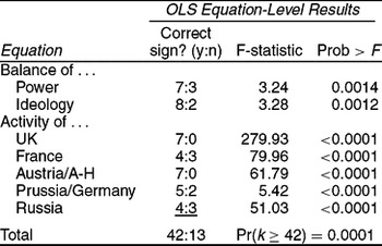
The results of the OLS estimation are summarized in Table 1 and demonstrate that, in addition to reasonable in-sample forecasts, the system of equations produces statistically significant results as well.Footnote 9 F-tests for the joint significance of coefficients in each equation all indicate significance exceeding the 0.01 level, usually substantially. Moreover, estimated coefficients, which represent our best guess about the value of the population coefficients, are of the expected sign in 42 instances and of the incorrect sign in only 13, an extremely unlikely (p=0.000057) outcome were the pattern of positive and negative coefficients simply produced by the equivalent of a coin-flip.
Summary of OLS Estimation of Full System of Equations

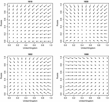
Because systems, even systems that are as straightforward as this one, are highly interactive, the predicted effects of the variables are unusually difficult to disentangle. They can, however, be illustrated, using phase portraits that describe the tendency of the model toward equilibrium for a subset of the variables at a given time. As a brief illustration, I have chosen to examine equilibrium tendencies of the United Kingdom and Russia, at four different points during the century.
Figure 1 presents this illustration. In 1818, the relative satisfaction of both states with the European continent that had been created by the Treaty of Vienna is apparent: neither has a compelling reason to upset the status quo, and in both states the model's prediction is a strong tendency toward inaction. By 1830, however, a substantial gap has opened up between Russian and British ideal points in the realm of liberalism, a fact brought to light by their nearly opposite reactions to the July Revolution and their divisions over the Belgian Revolution and soon codified in the Treaty of Münchengrätz and the Quadruple Alliance. Here, the model predicts an increase in activity for both states, though not an especially dramatic one. By the eve of the Crimean War in 1852, the salience of both systemic dimensions for both actors had dropped substantially (with the exception of the salience of ideology to the British, which remained the same). At the same time, liberalism had continued its spread, and Russia's ideal point had become slightly more illiberal—all of which points toward a slight decrease in Britain's demand for activity and a slight increase in Russia's. The resulting prediction, moderate and relatively equal levels of activity for both, suggests that neither was inactive enough to prevent a good target of opportunity for the other, and therefore that the onset of the crisis that led to the Crimean War more closely resembled a spiral than a failure of deterrence. Finally, by 1908 a dramatic upward shift (from below 0.2 to above 0.8 on the unit interval) in Britain's perception of the importance of the balance of power, combined with Germany's rapid rise and a continued British desire not to see Germany enter and surpass the ranks of the strongest states, prompted massive efforts on the part of the British, whereas Russia's somewhat greater indifference and willingness to countenance German power point toward intermediate levels of activity.
Phase Portrait of British and Russian Equilibrium Tendencies at Four Different Periods

Before moving on, it is worth examining the strength of the instruments, given that so-called “weak instruments” can produce even more finite-sample bias than the endogenous variables that they are meant to replace. Cameron and Trivedi (Reference Cameron and Trivedi2005, 104–10) suggest, as a rule of thumb, that the F-statistic for whether coefficients equal zero in a regression of the original activity variable on the instrument should exceed 10. It is reassuring to note that in four of five cases they do.Footnote 10 In the fifth case, that of Prussia, the statistic falls into the potentially problematic (as opposed to disastrous) ranges between 5 and 10. Accordingly, once the second-stage estimation below had been completed, I reestimated it using the original Prussian activity variable rather than the instrument, in order to determine whether the results were being driven by a biased instrument.
SECOND-STAGE RESULTS
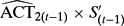
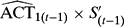
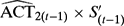
To recap, the spiral hypothesis argued that conflict should be most likely when two states' levels of security-related activity are balanced and there is considerable animosity between the two, whereas the deterrence hypothesis argued that conflict should occur when there is an imbalance of security-related activity between two such states. In terms of the model, the spiral hypothesis argues that the coefficients on 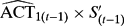 and
 should be null or negative, whereas the coefficient on
 should be positive. Conversely, the deterrence hypothesis argues that the coefficients on
 and
 should be positive, whereas the coefficient on
 should be negative.
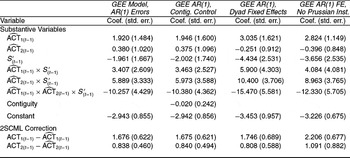
The second column of Table 2 contains the results of the GEE estimation. The data could hardly be less ambiguous: all three of the higher order coefficients that are relevant to both models have the sign predicted by the deterrence model, not by the spiral model. In the case of 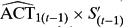 , which reflects the impact of a joint increase of these two variables when
 , the coefficient is positive, indicating that as the activity of state 1 and its dissimilarity with state 2 increase in tandem, the probability that a MID will break out increases. The coefficient on tells very much the same story—happily enough, as the state 1–state 2 designations are ideally arbitrary. The ratio of the standard error to the coefficient indicates strong statistical significance.
GEE Analysis of Relationship among Lagged, Predicted Levels of Activity, Dissimilarity of Alliance Portfolios, and MID Onset

Note: Robust standard errors, clustered by dyad, with AR(1) error structure; N = 980 for all tests.
The most striking evidence, however, can be found in the triple interaction of  , and S (t−1)′. If the spiral model is to be believed, joint increases in these three quantities should lead to an increase in the probability of conflict, whereas the deterrence model predicts a decrease. The sign and magnitude of the coefficient, as well as the ratio of coefficient to standard error, suggest a negative effect that is both substantively and statistically significant.
The third, fourth, and fifth columns describe the results of additional models that were run as checks on the robustness of the findings. They not only confirm the basic model's findings but also suggest even stronger results. Adding a control for contiguity (column 3) made essentially no difference at all in any of the other coefficients, and the coefficient on the contiguity variable proved to be substantively and statistically insignificant.Footnote 11 The inclusion of dyad fixed effects (column 4) produced no substantive change in the results—indeed, the coefficient on the main variables of interest maintained their signs and became substantially larger in magnitude. Replacing the Prussian instrument with the actual Prussian activity variable as a check on the effects of the weakness of the instrument, as described in the previous section (column 5), produced essentially similar results.
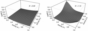
It is difficult, of course, to determine how large these substantive effects really are, taken together, without examining them. Accordingly, in Figure 2, I present a graph of the relationship among the activity of state 1, the activity of state 2, and the probability of MID onset, at the lowest and highest observed levels of S′. The parameters used for the graph were taken from the GEE AR(1) model with no fixed effects; as mentioned earlier, the parameters from the other models produce even stronger results. S′ captures antipathy, which is a necessary ingredient in both spiral and deterrence theories. Accordingly, the main figure of interest is the one on the right, and the results are impressive: the region around  , that is, the zone in which state 1's activity more or less equals that of state 2, never rises above an utterly negligible probability of conflict. When one of the two states is substantially more active than the other, the probability of conflict rises dramatically.
Predicted Effects of Levels of Activity on Probability of MID, at Lowest and Highest Observed Level of S′ (Model 1)

Given the observational nature of the data, the model's ability to do out-of-sample prediction is worth examining. Beck, King, and Zeng (Reference Beck, King and Zeng2004), in their examination of their model's out-of-sample performance vis-à-vis that of de Marchi, Gelpi, and Grynaviski (Reference de Marchi, Gelpi and Grynaviski2004), utilize percentage increase in the area underneath an ROC curve as a metric, which seems reasonable: that area corresponds to the empirical accuracy of the model, and a model that accurately captures a causal process that generalizes beyond the data that were used to generate the results should be able to improve on the accuracy of the null baseline (or on the accuracy of other models) when predicting out of sample. Beck, King, and Zeng's model, for example, successfully improves over the logit baseline by 2.5%, and over that of de Marchi et al.'s by 1.3%. Accordingly, I reserved the last 20 years of the data for prediction, reestimated the model based only on data from previous years, calculated predicted values for the out-of-sample period, and found a substantial improvement of 13.3% over a baseline fixed-effects probit containing only dyad dummies. (For a more detailed exercise in out-of-sample forecasting in the first-stage model, see [Braumoeller Reference Braumoeller, Albert, Cederman and Wendt2008b].)
In all, it seems that Clausewitz's (Reference Clausewitz1976, 82) aphorism about the only consideration that can constrain a state from taking military action being “the desire to wait for a better moment before acting” was an appropriate one: onset of disputes takes place for the most part when one state has let its guard down and the other tries to take advantage of the opportunity.
Dogs that Didn't Bark: Some Curious Non-MIDs
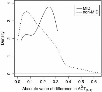
Although the second-stage analysis is valuable for its ability to give precise answers to specific theoretical hypotheses while controlling for such threats to inference as serial correlation and fixed effects, it nevertheless relies on some fairly strong assumptions to do so. It is therefore worth examining the data more closely to look for outliers or trends that are not obvious from the results. I calculated the absolute value of the differences in predicted levels of activity for both MID and non-MID cases, in all cases in which a fair degree of animosity existed, and plotted the densities of those distributions in Figure 3.Footnote 12 The figure confirms the general finding: non-MID cases are associated with lower differences in levels of activity, whereas MID cases are associated with higher differences in levels of activity. There is, however, an intriguingly long tail associated with the non-MID distribution, starting at around 0.4, that merits some attention.
Densities, for MIDs and Non-MIDs, of Absolute Value of the Differences in Predicted Levels of Activity, S′ > 0.5

The tail consists entirely of dyads involving two countries—Russia in the post-Crimea 1860s, and France in the latter half of the 1830s. Although space does not permit a thorough examination of these cases, both merit brief discussion. In the Russian case, Prussia and Austria, who presumably would have been best positioned to take advantage of Russia's exhaustion, had already done so in the Treaty of Paris, and both were occupied with Prussia's consolidation of Germany. In the second case, the conservative powers feared a highly active, revolutionary France in the 1830s. Nicholas I would have loved to have found an excuse to depose Louis-Philippe following the July Revolution; indeed, he raised an army in Poland to march to Paris and return the exiled Charles X to power. The recognition of Louis-Philippe by the states which lay between them, however, made this task substantially more difficult, and intervention by sea, especially in the face of British opposition, was implausible. Louis-Philippe nevertheless intentionally pursued a moderate foreign policy in order to deny the conservative monarchs an excuse to intervene. In the former case, Russia's period of near-isolationism happened to coincide with its potential opponents' preoccupation. In the latter, a curious (and, judging by the results regarding contiguity, relatively rare) situation arose in which geography prevented a clash between two states that would otherwise almost certainly have fought, and the threat of such a conflict dictated a passive rather than aggressive French policy.
Two interesting caveats suggest themselves in these cases. One, especially in multipolar systems, although conflict may imply a disparity of security-related activity, the converse is not necessarily true. States like Russia in the 1830s and Prussia in the 1860s might be prevented from capitalizing on an opportunity by geography or by satiety or by preoccupation with affairs elsewhere. Two, a general tendency such as the one documented here should not be mistaken for an iron law: for Louis-Philippe, despite the logic of deterrence theory, appeasement worked (though it was aided significantly by geography). By the same token, nothing in the results indicates that spirals cannot happen—just that they are comparatively quite rare.
CONCLUSION
This article has introduced a new systemic theory of international politics and demonstrated how, in combination with a dyadic theory of conflict, it can constitute a useful and plausible two-stage theory of conflict among European Great Powers in the nineteenth century. The argument at the heart of the theory is straightforward: the Great Powers attempt to manipulate the structure of the international system in a manner that is most conducive to the maintenance of general peace. Because their ideas regarding how best to do so differ, however, their attempts at implementing regulatory political regimes lead them to attempt to undermine one another's efforts. These attempts produce hostility and breakdowns in general deterrence, or onset of militarized interstate disputes, between Great Powers. They are most likely to do so when one Great Power in a hostile pair, by virtue of its relative inactivity, fails to deter the other.
Of equal interest, perhaps, is my conclusion that, in a head-to-head test, deterrence theory outperforms the spiral model as the dyadic half of this synthesis. This should not be taken as a claim that the spiral model has been falsified; rather, it suggests that deterrence-model conflicts are far more common in this period than are spiral-model conflicts. Figure 3 shows that conflicts consistent with the spiral model do indeed occur, but that they are a clear minority.
Three broader implications of this research deserve mention. First, I hope to have shown that systemic theory need not be either imprecise or irrelevant: rather than explaining the usual “small number of big things,” systemic theory can, in conjunction with a proximate theory of conflict, help to explain a big number of things, be they large or small. Second, systemic theory need not be ahistorical: the structure of the system is what states make of it, usually based on their own recent experience, and it is possible to allow for historical context without abandoning the systemic enterprise. Finally, the combination of a systemic and dyadic theories underscores the fact that theoretical synthesis is an area worthy of greater exploration. Levels of analysis and theoretical paradigms, which were originally intended to help scholars focus more carefully on the logic of their theories by temporarily “black-boxing” other sources of behavior, have instead become ossified ontologies, adherence to which requires categorically ruling out all other causes a priori. It need not be so: once developed, theories from different traditions can inform and enrich one another.
APPENDIX
Formalization of the Model
In a world of N Great Powers (1, . . ., n, . . ., N) and M issue dimensions, or spheres of interest (1,. . ., m, . . ., M), let a n denote the level of activity of state n, and let s m denote the current “state of the world” in sphere m. s and a are the state variables. Also let c nm represent a frequency distribution of constituency ideal points for state n on dimension m, and let νn(·) represent state n's preference aggregation function. ωnm represents the salience of issue-area m to the constituency of n—in other words, the degree to which changes in the distribution of goods relevant to issue m are deemed relevant to the national security of n. Finally, πn represents the realized capabilities of state n, scaled to 0 ≤ πn ≤ 1.
Of these, only νn(·) is relatively complex. Debates have played out in the public choice literature for decades regarding how preferences can be aggregated without running the risk of deadlock or cycling, and many reasonable answers have been offered for specific legislatures or categories of legislatures, but few can reasonably be applied to governments as diverse as Reagan's America and Tsarist Russia. The most reasonable general representation is one in which constituents support leaders with increasing probability as policies approach the constituents' ideal points, ideal points along one dimension are unrelated to ideal points along another, and leaders act to maximize their support.
Under those conditions, and assuming that probability distribution functions are continuous and strictly concave, the leader's governance problem becomes the maximization of  , where p i is the probability that constituent i will support the leader. In the most generic case, that in which constituents are equally weighted, is maximized at cnm, and because ideal points along one dimension are unrelated to ideal points along another, νn(c nm)=cnm ∀ m, and νn(c n) = cn: the aggregated preferences of the constituency of n collapse to the multidimensional mean (Persson and Tabellini Reference Persson and Tabellini2002, ch. 3).
s m constitutes the present state of the structure of the system: it contains all of the information at a given time about the distributions of power, ideology, and anything else that matters to the major states. ωnm determines the extent to which dimension m matters to state n, and νn(c nm) determines state n's collective “ideal point” along dimension m. Constituents demand action from the leadership in proportion to the extent that m matters to n and that the state of the world diverges from their collective ideal point. The former relationship is linear; in the latter case, the distance from the state of the world to the citizenry's ideal point is squared to reflect a traditional quadratic loss function. Leaders maximize their domestic support by acting to satisfy their constituency. The demands of their constituency are based on the distance between the collective ideal point and the status of the system, or νn(c nm)−s m, and the emphasis placed on that dimension of reality by the state's worldview, or ωnm. Therefore, the action taken by the leadership is described by

Finally, we need to calculate the instantaneous rate of growth (or decrease) in the state's activity by subtracting the existing level of demand from the right-hand side of the equation:
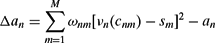
(where the time subscripts are dropped for notational convenience).
State activity should produce change in the system, in proportion to the level of activity. That level must be weighted by its realized capabilities, however; otherwise, actions taken by Switzerland will have the same impact as actions taken by the United States. Moreover, the impact of the state's activity should reflect the emphasis placed on the different dimensions of the system by that state's worldview. For a single state n and a single systemic dimension m, therefore,

Modeling multiple systemic dimensions follows in a straightforward way:

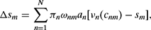
for all states n and all structural dimensions m.
Equations 4 and 5 from the formal model translate quite directly into estimable statistical equations. In fact, the equations resemble error-correction models of the sort described by Durr (Reference Durr1992), which leverage the strengths of differenced time series (namely, minimization of autocorrelation and unit root issues) while incorporating some information about levels in the adjustment term on the right-hand side. The nonlinearity of the right-hand side makes them a bit more complex than a standard error-correction model, however. For example, once the right-hand side has been multiplied out, the equation for one of the Great Powers—say, the UK, for the sake of illustration—would be
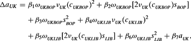
where a UK denotes the level of activity of the UK, ωUKBOP denotes the salience of the balance of power to the British, νUK(c UKBOP) represents the British ideal point with regard to the balance of power, s BOP denotes the present balance of power, LIB subscripts refer to the balance of political ideology rather than to the balance of power (see page 79, above, for historical background), and the βs are coefficients to be estimated. Four parallel equations describe the behavior of France, Austria/Austria-Hungary, Prussia/Germany, and Russia. Similarly, the equation for the balance of power would be

with two terms for each of the five Great Powers, and a second, parallel equation would describe the course of political liberalization on the continent.
The Survey
The survey asked respondents to gauge the quantities of interest and chart any changes in them over time. For example, to gauge the ideal points of leaders and their constituencies (defined as “the people legally empowered to emplace or remove” their leaders), respondents were asked, “If political elites could have had their way, what would the distribution of power in Europe have looked like? What about the preferences of their constituency, if such a group existed?” Answers for both leaders and constituents ranged from 1 (“All major states would have equal capabilities”) to 7 (“Even large inequalities of capabilities were fine as long as one state could still balance against threats”), along with “Don't know” and (in the case of constituencies) “Inapplicable.” To measure ω, the respondents were then asked, “As a measure of the general importance of the distribution of power in Europe to the national security of the state, how wide or narrow was the range of outcomes considered acceptable by political elites and (if applicable) by their constituents?” Answers ranged from 1 (“Nearly any distribution of capabilities would have been acceptable from the point of view of national security”) to 7 (“Only an extremely narrow range of outcomes would have been acceptable; anything outside of that range would constitute a threat.”), along with the same “Don't know” and “Inapplicable” options. Similar questions gauged opinions about the worldviews of leaders and constituencies on the distribution of ideas as well as about the general level of activity of the state (“Taking into account all forms of activity designed to increase national security, how active would you say the state's foreign policy was during this period?”) An initial draft of the survey was sent to a panel of five historical experts who offered valuable suggestions for revision as well as valuable insights into the ontological outlooks of historians.
The survey permitted respondents to select the state(s) and the period(s)—nineteenth century, interwar, or Cold War—about which they considered themselves to be most knowledgeable. As a result, unfortunately, more data was gathered on twentieth-century states than on nineteenth-century states, so a second wave of the survey was put into the field and respondents were asked specifically to address questions about states in earlier periods when possible. Finally, two of the respondents suggested that the questions about the Cold War could usefully have been augmented with an additional question about arms control, and in retrospect I agreed, so a third “minisurvey” was subsequently put into the field to ask follow-up questions regarding that issue area. In the end, there were 175 responses to the survey, each covering one Great Power over a span of 50 or (in the case of the interwar period) 40 years. Given that there were 18 such country-period combinations, there were an average of nearly ten respondents per data point. The data were then cleaned and averaged to produce a data set containing one quantity per question per country-year.
Expert-generated data are not uncommon in the study of political science (see, e.g., Budge Reference Budge2001 on expert data regarding political party positions, and Bueno de Mesquita Reference Bueno de Mesquita1998 on expert data on ideal points). Indeed, expert data have even been shown to be preferable to existing, objective data: Benoit and Laver (Reference Benoit and Laver2007), for example, compare the results of the Comparative Manifesto Project, a detailed and professional attempt to derive left-right party positions from content analysis of party platforms, to those of an expert survey on the same subject and find the latter to be more accurate. There are good reasons to consider the use of expert-generated data in international relations as well, the main one being the fact that survey data are designed to measure exactly the quantity of interest, while behavioral data are often very indirectly or imperfectly related to it.
Given the level of generality of the activity indicator, as well as the diversity of scholarly opinion, it is reasonable to wonder whether such a question can produce a reliable indicator. Cronbach's alpha is a worthwhile measure of intercoder reliability, with values below 0.60 considered clearly problematic, those in the 0.60–0.69 range borderline (acceptable by some scholars but not others), 0.70–0.79 acceptable, and 0.80 and above very strong. Because the number of coders varies from one country-period to the next, however, a single test statistic is difficult to calculate. To overcome this difficulty I calculated the average of all of the alpha statistics for all of the country-periods in the survey, weighted by the number of coders in each. The result was an aggregate Cronbach's alpha of 0.72, indicating a reliability that falls into the unambiguously acceptable range.
It is also worth asking whether existing behavioral data on levels of state activity might not be more valid indicators than the data derived from the expert survey. Because there is no a priori best indicator to use as a “gold standard,” the best test of validity is to compare the activity variable introduced here to a variable derived from a range of more objective, behavioral indicators, and to ask which variable does a better job of capturing known events (wars, arms races, and periods of increased tension).
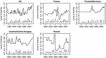
Toward that end, I conducted a factor analysis on five indicators of state activity—number of military personnel in given year, raw military expenditures in given year, number of allies in a given year, total number of other states with which the state was engaged in a MID in a given year, and the sum of hostility levels across all MIDs in a given year (the last to distinguish more serious from less serious disputes). The goal was to capture unilateral, multilateral, and aggressive behavior, in the hopes that doing so would be the most flexible way to produce a comprehensive indicator of security-related activity. I used principal-components factor analysis. Initially, two factors passed the threshold for retention, with eigenvalues of 2.34 and 1.34; in order to create a single measure, I rotated the factors (Varimax rotation) and retained the first factor. Using either or both of the two original factor scores does not improve face validity, and using the log of military expenditures makes no substantive difference. I then scaled both the measure derived from the factor analysis and the expert-generated data to the unit interval and plotted them together in Figure 4 as a way of getting at the face validity of the two indicators.
Levels of State Activity Derived from the Expert Survey (Black Line) and Factor Analysis of Unilateral and Multilateral Behavior (Grey Line)

The figure suggests very strongly that the expert-generated data are as good as, and quite possibly much better than, the behavioral data at capturing trends in security-related activity. The Crimean War, which stands out as a prominent burst of activity in the 1850s, shows up as a plateau for the UK, France, and, most prominently, Russia in the expert data; in the behavioral data, the war does not stand out at all. The generally increasing levels of European hostility starting (for lack of a better date) around 1890, when Caprivi replaced Bismarck and Germany abandoned the Reinsurance Treaty, and accelerating through the naval race sparked by the Dreadnought in 1906, show up clearly in the historians' data from the beginning, but prior to 1913 the aggregated behavioral indicator suggests anything but escalating tension—in fact, in every state save perhaps for Austria/Hungary and Russia it suggests, if anything, the opposite. At times, the data do agree: France, for instance, experiences a spike in activity during the Franco-Prussian War in both series (though it hardly stands out in the behavioral data), the Russo-Turkish war in the late 1870s shows up in both (though diffused somewhat in the behavioral data), and Russia's temporary withdrawal from European politics following its defeat in the Crimea is reasonably represented in both. Nevertheless, at least in the most objectively clear cases, when the data disagree, those from the historians' survey have considerably greater face validity.
Space permits only the briefest speculation as to the reasons for these differences. The behavioral data, it seems to me, are not always consistently related to the underlying concept that they are meant to capture. In a multilateral state, an absence of alliances indicates low levels of activity; in a highly unilateral state, however, an absence of alliances could be associated with any level of activity. A state that relies on strong allies might spend little on its own defense even if it is highly active. A state might be very active for ten years but only experience MIDs in 2 of those 10 years, so the absence of MIDs is an ambiguous indicator. (It might be possible to use a moving average rather than a yearly measure to mitigate this problem, but doing so would induce massive serial correlation, produce measures that are highly dependent on the number of years used, arbitrarily, for the average, and be inherently unable to pick up transition points—in all, a bad trade.) Worse, many of these behaviors are indicative, to some degree, not of an increasingly active foreign policy but rather of an attempt to maintain internal order during an era of uprisings and revolution. In short, the relationship of the behavioral indicators to activity is highly contextual, depending heavily on the state and period in question, and the contextual knowledge needed to construct a more valid indicator would most likely have to come from the same historians whose efforts produced the expert index of activity.
Another way to explore the validity of the activity measure is to ask whether dyadic gaps in activity really correspond to the sorts of conflicts that they should: that is, do the cases that are consistent with the spiral (deterrence) model in the data actually correspond to cases of spirals (deterrence failures) in the real world? This is a difficult question to answer for three reasons. First, there is no obvious theoretical or empirical cutoff between deterrence failures and spirals: it would be convenient if, say, we could know that a gap of more than 0.15 between the activity of one state and that of another was consistent with deterrence theory, but nothing permits such a claim. Second, instruments are correlated with the quantity of interest, but not perfectly; therefore, even if such a cutoff were to exist, one would expect exceptions. The inference about deterrence vs. spiral models doesn't rest on individual cases but rather on the relationship between activity levels and initiation across many cases. Finally, historians continue to argue over the question of whether even very prominent cases should be considered spirals or deterrence failures, so no consistent, objective referent exists against which these cases might be checked.
We might still gain something, however, by examining the cases at the tails of the distribution—those MIDs in which gaps in activity are either very large or very small. If the activity measure captures what it should, MIDs with large gaps between the activity levels of participants should tend to be the result of deterrence failures, and those with small gaps should tend to be the result of spiral processes—at least, to the extent that we are able to agree on the coding of these events.
The results bear out this expectation nicely. The Crimean War was, famously, a pointless war, a minor French attempt to score domestic political points by meddling in the politics of the Holy Lands that spiraled into a massive and senseless slaughter; it tops the list of small-gap MIDs. Next is the Dogger Bank incident of 1904, a bit difficult to code because the Russians mistook British trawlers for Japanese warships (though the trawlers surely did not attempt to deter the attack). Third on the list is the imposition of a settlement in Belgium in 1832 following the Belgian Revolution—a case in which most of Europe feared that France would attempt to expand its influence, and France feared that the British or the Prussians would do the same. Next is the British–German dyad at the onset of the First World War, a contested case in general because of German intentions, but the naval arms race and the fact that even a culpable, scheming Germany hoped for and expected British noninvolvement make this dyad far more consistent with the spiral model than others. The fifth case on the list is the Second Morocco Crisis, a case in which no one sought conflict but a large difference in perceptions of “normal” standards for reciprocal compensation in colonial areas led to a serious dispute.
The cases with the largest gaps are not as historically prominent but lend themselves to a far lesser degree to a spiral interpretation. The Near Eastern Crisis of 1833 occurred because Nicholas saw an opportunity to isolate France and extend Russian influence in the Ottoman Empire, and he took it. (Remember that in these cases the breakdown of general deterrence, for example, Nicholas' decision to initiate a crisis, is the phenomenon of interest—not the success or failure of immediate deterrence that sometimes follows.) Two conflict dyads from the Second Syrian War dispute fall into this category as well, and here, France again attempted and failed to forestall pro-Ottoman intervention by the remaining Great Powers. The Panjdeh (or Penjdeh) Dispute of 1885 is perhaps the most questionable of the lot: it certainly bears the hallmarks of a deterrence failure, but the codings indicate that the Russians failed to deter the British from initiating a crisis. If we view Russian expansion into Central Asia as a normal process of late nineteenth-century colonial behavior, one that they sought to prevent the British from interfering with, they certainly failed to do so in this instance; but the British would be more apt to interpret Panjdeh as a case of their own failure to deter the Russians from coming too close to India. Finally, Russia clearly failed to prevent British involvement in the Russo-Turkish War in 1877: it had ensured Austria's benevolent neutrality via the Treaty of Budapest in January, but when war came the British sent a memorandum spelling out their own conditions for noninvolvement in the conflict. Again, informed opinions may differ on the interpretations of a few of these events, but even this brief overview of the more extreme cases bolsters our confidence that the variable is measuring what it is supposed to measure.
Finally, given that the goal of the second stage of this study is to understand how activity relates to conflict, it is worth asking whether there is any danger of circularity—that is, whether the expert data are simply a restating of the dependent variable in the second stage. Remember that, to minimize this danger, activity at time t−1 was used to predict conflict at time t. Still, it is possible that, despite the best intentions of historians, the onset of a large-scale conflict in 1853 or 1914 would influence assessments of the relevant states' levels of activity in 1852 or 1913. Two pieces of evidence mitigate against such a claim, however. First, the survey data in Figure 4 show pronounced, sometimes dramatic, peaks that correspond very closely to conflicts. Second, if historians were imputing higher levels of activity to involved states prior to conflict, those states' activity scores would be raised across the board and would therefore tend either to remain the same or to converge. To illustrate, imagine that the real scores for two states, a i and a j, are adjusted upward by hindsight. If they are both adjusted upward equally, by x units, the difference between the two remains the same. If the activity of the more-active state is adjusted upward to a lesser degree, either because the state is already seen as quite active or because the scale is bounded (imagine that each is adjusted upward by  ), the gap narrows. Therefore, hindsight would most likely produce either no difference in the second-stage findings or a bias toward the spiral model argument. Because the second-stage findings support the deterrence over the spiral model, elimination of such a bias could only strengthen the results.
 . The general outlines of the graph are robust to reasonably large changes in the cutoff value. The densities look a bit odd because I have specified that they be cut off at their minimum and maximum values; not doing so creates the illusion of tails, which is confusing.



Comments
No Comments have been published for this article.