1 Introduction
Understanding wall-bounded turbulent flows is a long-standing challenge because of their complex and chaotic nature. The presence of a wall not only induces the formation of a thin shear layer close to the wall, known as the turbulent boundary layer (TBL), where most of the energy consumption occurs in modern vehicles and pipelines, but also separates the TBL into different layers composed of multiscale fluid motions. These multiscale phenomena can be characterized in terms of the friction Reynolds number (
 $Re_{\unicode[STIX]{x1D70F}}=\unicode[STIX]{x1D6FF}u_{\unicode[STIX]{x1D70F}}/\unicode[STIX]{x1D708}$
), which is the ratio of the viscous length scale
 $\unicode[STIX]{x1D708}/u_{\unicode[STIX]{x1D70F}}$
(
 $\unicode[STIX]{x1D708}$
is the kinematic viscosity, and
 $u_{\unicode[STIX]{x1D70F}}$
is the friction velocity) and the flow thickness
 $\unicode[STIX]{x1D6FF}$
. Although much progress has been achieved in characterizing the onset of turbulence (Hof et al.
Reference Hof, van Doorne, Westerweel, Nieuwstadt, Faisst, Eckhardt, Wedin, Kerswell and Waleffe2004; Avila et al.
Reference Avila, Moxey, de Lozar, Avila, Barkley and Hof2011) and fully turbulent flows at low
 $Re_{\unicode[STIX]{x1D70F}}$
(Kawahara, Uhlmann & Van Veen Reference Kawahara, Uhlmann and Van Veen2012), high
 $Re_{\unicode[STIX]{x1D70F}}$
turbulence that arises in engineering devices and atmospheric winds (
 $Re_{\unicode[STIX]{x1D70F}}=O(10^{4{-}6})$
) is an open challenge due to the wide range of scales that govern the transport of mass, momentum and heat (Smits, McKeon & Marusic Reference Smits, McKeon and Marusic2011; Jiménez Reference Jiménez2012; Barkley et al.
Reference Barkley, Song, Mukund, Lemoult, Avila and Hof2015).
One approach to the characterization of these multiscale phenomena of TBLs is to examine the organized motions that retain their spatial coherence for relatively long periods, known as eddies or coherent structures, because these structures are responsible for the dynamical mechanisms and turbulence statistics (Robinson Reference Robinson1991; Adrian Reference Adrian2007). The dominant coherent structures in the buffer layer are low-speed streaks and quasi-streamwise vortices (Kline et al.
Reference Kline, Reynolds, Schraub and Runstadler1967) that are generated via a self-sustaining cycle (Hamilton, Kim & Waleffe Reference Hamilton, Kim and Waleffe1995). Above the buffer layer, the coherent structures are larger and more complex due to the presence of various scales. In this region, the mean streamwise velocity (
 $\overline{U}$
) follows a logarithmic profile along the wall-normal distance
 $y$
(Millikan Reference Millikan1938):
 $$\begin{eqnarray}\overline{U}^{+}=\unicode[STIX]{x1D705}^{-1}\ln (y^{+})+A,\end{eqnarray}$$
where
 $\overline{U}^{+}=\overline{U}/u_{\unicode[STIX]{x1D70F}}$
,
 $y^{+}=u_{\unicode[STIX]{x1D70F}}y/\unicode[STIX]{x1D708}$
,
 $\unicode[STIX]{x1D705}$
is the von Kármán constant,
 $A$
is an additive constant and the overbar indicates an ensemble average. The logarithmic profile in (1.1) represents that the only relevant scales in this region are
 $y$
and
 $u_{\unicode[STIX]{x1D70F}}$
(i.e.
 $\unicode[STIX]{x2202}\overline{U}/\unicode[STIX]{x2202}y\sim u_{\unicode[STIX]{x1D70F}}/y$
). At high Reynolds numbers, most of the bulk production and velocity drop originate from the logarithmic layer (Smits et al.
Reference Smits, McKeon and Marusic2011; Jiménez Reference Jiménez2012). Townsend (Reference Townsend1976) deduced a model for energy-containing eddies in the logarithmic layer whose sizes scale with
 $y$
; these structures are attached to the wall and are self-similar. By assuming that the logarithmic layer consists of the superposition of the attached eddies and that the variation of the Reynolds shear stress across the layer is small compared to the viscous stress, the turbulence intensities (
 $\overline{u_{i}^{2}}$
) can be expressed as
 $$\begin{eqnarray}\displaystyle & \displaystyle \overline{u^{2}}^{+}=B_{1}-A_{1}\ln (y/\unicode[STIX]{x1D6FF}), & \displaystyle\end{eqnarray}$$
 $$\begin{eqnarray}\displaystyle & \displaystyle \overline{w^{2}}^{+}=B_{2}-A_{2}\ln (y/\unicode[STIX]{x1D6FF}), & \displaystyle\end{eqnarray}$$
 $$\begin{eqnarray}\displaystyle & \displaystyle \overline{v^{2}}^{+}=B_{3}, & \displaystyle\end{eqnarray}$$
 $u$
(
 $=u_{1}$
),
 $v$
(
 $=u_{2}$
) and
 $w$
(
 $=u_{3}$
) are the streamwise, spanwise and wall-normal velocity fluctuations, respectively, and
 $A_{j}$
(
 $j=1$
, 2) and
 $B_{i}$
are constants;
 $A_{j}$
is the Townsend–Perry constant, which is expected to be universal (Marusic et al.
Reference Marusic, Monty, Hultmark and Smits2013). Here, the wall-parallel components follow the logarithmic variation, whereas the wall-normal component is constant. The inviscid assumption for self-similar eddies leads to the logarithmic behaviour in (1.2a
) and (1.2b
) and the impermeable condition for the wall-normal component gives rise to (1.2c
). Perry & Chong (Reference Perry and Chong1982) extended this hypothesis by proposing that there are hierarchies of geometrically similar eddies with a probability distribution function (PDF) that is inversely proportional to their height. Based on this approach, they derived the logarithmic variation of
 $\overline{U}$
(1.1) and
 $\overline{u_{i}^{2}}$
(1.2a
) and (1.2b
) simultaneously in the context of the attached-eddy hypothesis. Additionally, they predicted the emergence of a
 $k_{x}^{-1}$
(
 $k_{x}$
is the streamwise wavenumber) region in the spectrum that is the spectral signature of the attached eddies. In this regard, the attached-eddy hypothesis is a unified theory that links the asymptotic behaviours of the turbulence statistics of high-Reynolds-number flows.
Subsequently, several studies (Perry, Henbest & Chong Reference Perry, Henbest and Chong1986; Perry & Marusic Reference Perry and Marusic1995; Marusic & Kunkel Reference Marusic and Kunkel2003) have refined the model of Perry & Chong (Reference Perry and Chong1982) in order to test Townsend’s hypothesis, but their Reynolds numbers are not sufficiently high to establish the logarithmic region. Nickels et al. (Reference Nickels, Marusic, Hafez and Chong2005) demonstrated the presence of the
 $k_{x}^{-1}$
region in the streamwise velocity spectrum (
 $\unicode[STIX]{x1D6F7}_{uu}$
). The coexistence of the logarithmic regions for
 $\overline{U}$
and
 $\overline{u^{2}}$
was observed at
 $Re_{\unicode[STIX]{x1D70F}}=O(10^{4{-}5})$
(Hultmark et al.
Reference Hultmark, Vallikivi, Bailey and Smits2012; Marusic et al.
Reference Marusic, Monty, Hultmark and Smits2013). Through a spectral analysis over the same range of
 $Re_{\unicode[STIX]{x1D70F}}$
, Vallikivi, Ganapathisubramani & Smits (Reference Vallikivi, Ganapathisubramani and Smits2015) observed a plateau region (i.e.
 $k_{x}\unicode[STIX]{x1D6F7}_{uu}/u_{\unicode[STIX]{x1D70F}}^{2}\approx$
const.) in the vicinity of the outer peak, which can contribute to the logarithmic variation in
 $\overline{u^{2}}$
. For the spanwise component, Jiménez & Hoyas (Reference Jiménez and Hoyas2008) observed the logarithmic variation at
 $Re_{\unicode[STIX]{x1D70F}}\approx 2000$
. Recently, Marusic & Monty (Reference Marusic and Monty2018) has reviewed Townsend’s hypothesis by focusing on attached-eddy modelling for high
 $Re_{\unicode[STIX]{x1D70F}}$
. Nevertheless, the central question that has not been resolved is as follows: what is the actual structure in the fully turbulent flow that corresponds to an attached eddy and forms the logarithmic region? Although Townsend (Reference Townsend1976) and Perry & Chong (Reference Perry and Chong1982) proposed a particular shape of eddies based on the flow visualization, these structures were modelled to formulate the inverse power-law PDF and the constant shear stress. Additionally, the presence of the
 $k_{x}^{-1}$
region does not necessarily indicate the presence of an attached structure, because a coherent motion can carry energy with a broad range of wavenumbers (Nickels & Marusic Reference Nickels and Marusic2001) and the wavenumber at a given
 $y$
does not reflect whether that motion is attached to the wall or is a part of detached one (Jiménez Reference Jiménez2013).
To overcome these limitations, clusters of vortices (del Álamo et al.
Reference del Álamo, Jiménez, Zandonade and Moser2006) and three-dimensional sweeps/ejections (Lozano-Durán, Flores & Jiménez Reference Lozano-Durán, Flores and Jiménez2012) were identified in direct numerical simulation (DNS) data of channel flows. These structures can be classified as either wall-attached or wall-detached based on their minimum distances from the wall. The former are self-similar and statistically dominant structures in the logarithmic layer. Morrill-Winter, Philip & Klewicki (Reference Morrill-Winter, Philip and Klewicki2017) and Fiscaletti, de Kat & Ganapathisubramani (Reference Fiscaletti, de Kat and Ganapathisubramani2018) found that the size of the structures associated with the intense Reynolds shear stress increases with
 $y$
. Hwang (Reference Hwang2015) found self-similar statistical motions with respect to
 $y$
in a large-eddy simulation that restricted the spanwise length scale of motions. By using a proper orthogonal decomposition, Hellström, Marusic & Smits (Reference Hellström, Marusic and Smits2016) found that the azimuthal length scales of the energetic modes are proportional to the distance from the wall. In addition, Baars, Hutchins & Marusic (Reference Baars, Hutchins and Marusic2017) reported a self-similar region in the linear coherence spectrum, in which the coherence magnitude can be quantified in terms of a single streamwise/wall-normal aspect ratio. Although these identified coherent motions are reminiscent of Townsend’s attached eddies in the sense of self-similarity, it has not yet been shown how they contribute to the formation of the logarithmic behaviour in
 $\overline{u^{2}}$
and
 $\overline{w^{2}}$
.
The objective of the present study is to identify the self-similar coherent structures satisfying the attached-eddy hypothesis by examining the DNS data of zero-pressure-gradient TBL at
 $Re_{\unicode[STIX]{x1D70F}}\approx 1000$
. In this approach, we extracted the clusters of the velocity fluctuations (
 $u_{i}$
) in order to identify a group of
 $u_{i}$
clusters over a wide range of scales that are attached to the wall and are self-similar. In particular, the population density of the attached
 $u$
clusters is inversely proportional to their height. We then reconstruct the turbulence intensities by performing the superposition of the identified structures. The logarithmic behaviours of the wall-parallel components are then verified by using the indicator function, which has not been achieved experimentally. Further, we focus on the
 $u$
clusters in order to explore the hierarchical nature of the structures. The wall-normal distribution of the instantaneous streamwise velocity contained in the objects shows step-like jumps, representing the zones of roughly constant uniform momentum. In addition, we observe that the magnitude of the near-wall peak in the streamwise turbulence intensity carried by the attached clusters of
 $u$
increases logarithmically with increasing their heights. The present results not only support the attached-eddy hypothesis but also provide direct evidence regarding the presence of the attached structures in instantaneous flow fields, even at the moderate-Reynolds-number TBL.
2 Computational details
The DNS data of the TBL (Hwang & Sung Reference Hwang and Sung2017a
; Yoon, Hwang & Sung Reference Yoon, Hwang and Sung2018) are used in the present study. The DNS was performed using the fractional step method of Kim, Baek & Sung (Reference Kim, Baek and Sung2002) to solve the Navier–Stokes equations for incompressible flow. The computational domain is
 $2300\unicode[STIX]{x1D6FF}_{0}\times 100\unicode[STIX]{x1D6FF}_{0}\times 100\unicode[STIX]{x1D6FF}_{0}$
, where
 $\unicode[STIX]{x1D6FF}_{0}$
is the inlet boundary layer thickness, in the streamwise (
 $x$
), wall-normal (
 $y$
) and spanwise (
 $z$
) directions, respectively, and the associated components of the velocity fluctuations are
 $u$
,
 $v$
and
 $w$
; details of the DNS and its validation are provided in Hwang & Sung (Reference Hwang and Sung2017a
). We used a total of 2430 instantaneous flow fields at
 $Re_{\unicode[STIX]{x1D70F}}=980$
with the streamwise length (
 $L_{x}$
) of
 $11.7\unicode[STIX]{x1D6FF}$
; the spanwise length (
 $L_{z}$
) is
 $3.2\unicode[STIX]{x1D6FF}$
and
 $\unicode[STIX]{x1D6FF}$
is the 99 % boundary layer thickness. Here, the instantaneous flow fields are collected in the time step interval of 2.54 viscous time units (
 $0.065\unicode[STIX]{x1D6FF}/U_{\infty }$
); the total averaging time to compute identified structures is 6170 viscous time units (
 $157.95\unicode[STIX]{x1D6FF}/U_{\infty }$
). Across the domain, the Reynolds-number effect is negligible because
 $Re_{\unicode[STIX]{x1D70F}}$
ranges from 913 to 1039.
In the present study, the fluctuating velocity components are defined by considering the height of the turbulent/non-turbulent interface (TNTI) (Kwon, Hutchins & Monty Reference Kwon, Hutchins and Monty2016). The wall-normal distance of the instantaneous TNTI
 $\unicode[STIX]{x1D6FF}_{t}(x,z)$
is defined using the kinetic energy criteria proposed by Chauhan et al. (Reference Chauhan, Philip, de Silva, Hutchins and Marusic2014). Here, we used all the velocity components to obtain the local turbulent kinetic energy (
 $\tilde{k}$
) in a frame of reference moving with
 $U_{\infty }$
over a
 $3\times 3\times 3$
grid. We employed the threshold of
 $\tilde{k}=0.09$
, which is slightly lower than that of Chauhan et al. (Reference Chauhan, Philip, de Silva, Hutchins and Marusic2014). As a result, the mean of the TNTI height is
 $\overline{\unicode[STIX]{x1D6FF}_{t}}=0.88\unicode[STIX]{x1D6FF}$
, which is close to that reported in Jiménez et al. (Reference Jiménez, Hoyas, Simens and Mizuno2010) who defined the TNTI height in terms of the enstrophy. Note that the results in the present work remained qualitatively unchanged regardless of the TNTI threshold because we focus on the structures within the turbulent region only (Hwang & Sung Reference Hwang and Sung2017b
). The streamwise velocity fluctuations based on the Reynolds decomposition are positive when
 $\unicode[STIX]{x1D6FF}_{t}$
is lower than
 $\unicode[STIX]{x1D6FF}$
. In other words, although these positive-
 $u$
regions are located in the free-stream region (the non-turbulent region), they are regarded as the turbulent regions. We define the velocity fluctuations
 $u_{i}=U_{i}-\overline{U_{i}}(y,\unicode[STIX]{x1D6FF}_{t})$
to prevent this contamination. Here,
 $\overline{U_{i}}(y,\unicode[STIX]{x1D6FF}_{t})$
is the conditional mean velocity, which is a function of the wall-normal distance and the local TNTI height (Kwon et al.
Reference Kwon, Hutchins and Monty2016).
Clusters of velocity fluctuations (
 $u_{i}$
) at
 $Re_{\unicode[STIX]{x1D70F}}=980$
. The red and blue isosurfaces indicate the positive and negative fluctuations,
 $u_{i}(\boldsymbol{x})=\pm 1.5u_{rms,i}(y,\unicode[STIX]{x1D6FF}_{t})$
, respectively, in the instantaneous flow field: (a)
 $u$
, (b)
 $w$
and (c)
 $v$
. The brightness of the colour indicates the distance from the wall. Here, clusters that cross the edges of the streamwise and spanwise domains were excluded in order to show the full size of each cluster.

(a) Percolation behaviour of the identified clusters; the variation of the volume of the largest cluster (
 $V_{m}$
) normalized by the total volume of the clusters
 $V_{t}$
,
 $V_{m}/V_{t}$
, and the ratio of the total number of the clusters (
 $N$
) to the maximum
 $N$
over
 $\unicode[STIX]{x1D6FC}$
(
 $N_{m}$
),
 $N/N_{m}$
. (b) The number of clusters per unit wall-parallel area as a function of
 $y_{min}$
and
 $y_{max}$
. The colour contour indicates the distribution of the
 $u$
clusters, and the red and orange line contours represent the
 $w$
and
 $v$
clusters, respectively, with a contour level of 0.003.

The clusters of positive or negative fluctuations are the groups of connected points satisfying
 $$\begin{eqnarray}u_{i}(\boldsymbol{x})>\unicode[STIX]{x1D6FC}u_{rms,i}(y,\unicode[STIX]{x1D6FF}_{t})\quad \text{or}\quad u_{i}(\boldsymbol{x})<-\unicode[STIX]{x1D6FC}u_{rms,i}(y,\unicode[STIX]{x1D6FF}_{t}),\end{eqnarray}$$
where
 $u_{rms,i}$
is the root mean square of the corresponding
 $u_{i}$
and
 $\unicode[STIX]{x1D6FC}$
is the threshold. Figure 1 shows the isosurfaces of
 $u$
,
 $w$
and
 $v$
in the instantaneous flow field. As seen, the shapes of these structures are complex: some of them are attached to the wall whereas others are distributed far above the wall and have a small volume. In particular, the structures of the cross-stream components are pronounced at the edge of the boundary layer; the lighter colour denotes structures with a wall-normal distance close to
 $\unicode[STIX]{x1D6FF}_{t}$
. In addition, in contrast to figure 1(b,c) there are long meandering structures of
 $u$
(the darker red or blue isosurfaces) in figure 1(a), which are discussed further in § 3. To characterize the irregular shapes of the
 $u_{i}$
clusters (figure 1), the connectivity of
 $u_{i}$
was defined based on the six orthogonal neighbours of each node in Cartesian coordinates (Moisy & Jiménez Reference Moisy and Jiménez2004; del Álamo et al.
Reference del Álamo, Jiménez, Zandonade and Moser2006; Lozano-Durán et al.
Reference Lozano-Durán, Flores and Jiménez2012). Using the connectivity rule, the contiguous points can be determined at a given node. Thus, we could measure the sizes of clusters and obtain the velocity information over a bounded volume for each object without making an a priori assumption or applying a filter. However, the detection of the structure depends on the threshold value
 $\unicode[STIX]{x1D6FC}$
. When
 $\unicode[STIX]{x1D6FC}$
is low, new contiguous points are detected and some of them merge with the previously identified regions. Figure 2(a) shows the variation with
 $\unicode[STIX]{x1D6FC}$
in the ratio of the maximum volume of the cluster (
 $V_{m}$
) to the total volume of the clusters (
 $V_{t}$
). Here,
 $V_{m}$
and
 $V_{t}$
are the sum of the corresponding clusters for negative and positive fluctuations. The black line indicates the total number of the clusters (
 $N$
) normalized by its maximum (
 $N_{m}$
), which appears at
 $\unicode[STIX]{x1D6FC}_{m}\approx 1.4$
for
 $u$
and
 $\unicode[STIX]{x1D6FC}_{m}\approx 1.6$
for
 $v$
and
 $w$
. At
 $\unicode[STIX]{x1D6FC}>1.7$
, the clusters of intense
 $u_{i}$
with very small volume are identified. The volume ratios of
 $v$
and
 $w$
clusters converge to 0.05 and 0.07, respectively, representing that the intense structures for the cross-stream component have very small volumes:
 $V_{m}/V_{t}\approx 0.13$
for
 $u$
. As
 $\unicode[STIX]{x1D6FC}$
decreases,
 $V_{m}/V_{t}$
increases significantly and converges to 1. Many new clusters are generated and amalgamated simultaneously, and the amalgamation of the clusters becomes dominant at
 $\unicode[STIX]{x1D6FC}<\unicode[STIX]{x1D6FC}_{m}$
, which leads to the decrease in
 $N/N_{m}$
. This result is consistent with the percolation transition in turbulence structures, such as arises for vortical structures (Moisy & Jiménez Reference Moisy and Jiménez2004; del Álamo et al.
Reference del Álamo, Jiménez, Zandonade and Moser2006) and ejection/sweep structures (Lozano-Durán et al.
Reference Lozano-Durán, Flores and Jiménez2012). The threshold
 $\unicode[STIX]{x1D6FC}=1.5$
(vertical dashed line) was chosen based on the percolation transition of the clusters; the results remain qualitatively unchanged in the vicinity of the threshold (see appendix A).
In order to identify the wall-attached structures, the minimum and maximum
 $y$
(
 $y_{min}$
and
 $y_{max}$
) for each cluster are measured from the wall. Figure 2(b) shows the number of clusters per unit wall-parallel area (
 $L_{x}\times L_{z}$
) according to
 $y_{min}$
and
 $y_{max}$
. Here, the colour contour indicates the distribution of the
 $u$
clusters and the inserted line contours represent the distributions of the
 $w$
(red) and
 $v$
(orange) clusters. There are two distinct regions, yielding that the clusters are classified into two groups: wall-attached structures with
 $y_{min}^{+}\approx 0$
and the detached structures with
 $y_{min}^{+}>0$
. The minimum wall-normal distance of the wall-attached group is located at
 $y_{min}^{+}=0.08$
, which is the grid point closest to the wall in the present DNS data. Although previous studies (del Álamo et al.
Reference del Álamo, Jiménez, Zandonade and Moser2006; Lozano-Durán et al.
Reference Lozano-Durán, Flores and Jiménez2012) classified the clusters of the vortex and Reynolds shear stress into wall-attached and wall-detached groups based on
 $y_{min}^{+}\approx 20$
, we defined the attached structures of the velocity fluctuations with
 $y_{min}^{+}\approx 0$
because most of the clusters within
 $y_{min}^{+}<20$
are at
 $y_{min}^{+}\approx 0$
(88 %, 76 % and 78 % for
 $u$
,
 $w$
and
 $v$
, respectively). In addition, we can obtain the turbulent intensity carried by the attached structures according to their height (
 $l_{y}$
) without any interpolation since
 $l_{y}=y_{max}$
rather than
 $l_{y}=y_{max}-y_{min}$
. In other words, the attached structures identified in the present study are physically adhered to the wall. As a result, these structures show the characteristics of the logarithmic layer as well as of the buffer layer; this point is discussed further in §§ 4 and 5.
Before addressing the characteristics of the attached structures, it is worthwhile discussing the term ‘attached’ used in the attached-eddy hypothesis (Townsend Reference Townsend1976). Townsend conjectured that the main energy-containing motions in the constant shear stress layer (i.e. at an extremely high Reynolds number) are attached to the wall and thus the eddies are inviscid. As a result, the slip boundary condition can be assumed for the wall-parallel velocity components (i.e.
 $u$
and
 $w$
) since the hypothesis is valid far above the region where the viscosity is dominant. For the wall-parallel component, Hwang (Reference Hwang2016) showed that the energy-containing motions in the form of Townsend’s attached eddies penetrate into the region close to the wall (i.e. these are the footprints reported in Hutchins & Marusic Reference Hutchins and Marusic2007a
,Reference Hutchins and Marusic
b
) and that the near-wall penetration of these motions exhibits the inner-scaling behaviour. In this respect, the present definition of the attached clusters does not contradict the attached-eddy hypothesis but rather their near-wall parts could contain the viscous effect, which is not considered in the attached-eddy hypothesis (see further § 5).
The number and volume fractions with respect to the total number and total volume of all the identified
 $u_{i}$
clusters.

Although the wall-normal velocity is affected by the impermeable condition, which leads to an absence of the logarithmic variation of its intensity profile in a sense of the attached-eddy hypothesis, we can observe the attached structures of
 $v$
in figure 2(b). However, this is not so surprising, given the identification criteria of the present approach (2.1). We used the root mean square of the velocity fluctuations (
 $u_{rms,i}$
), which varies with
 $y$
. Hence,
 $u_{rms,i}$
reaches zero at the wall, and in particular the value of the wall-normal component is much less than that of the wall-parallel components in the near-wall region. This behaviour is also related to the presence of the attached clusters of ejections/sweeps (Lozano-Durán et al.
Reference Lozano-Durán, Flores and Jiménez2012) since the Reynolds shear stress is the product of
 $u$
and
 $v$
.
In contrast to the cross-stream component, there is a weak peak at
 $y_{min}^{+}\approx 7$
and
 $y_{max}^{+}\approx 50$
for the
 $u$
clusters in figure 2(b). These structures can be the fragments of large attached structures or an object that is developing into a larger one; their number of occurrence is less than 0.011 per unit wall-parallel area. In the present work, we focus on the attached structures with heights that vary from the near-wall region to
 $\unicode[STIX]{x1D6FF}$
. The number and volume fractions of the identified clusters are summarized in table 1. Here, we only consider the
 $u_{i}$
clusters with volume larger than
 $30^{3}$
wall units (del Álamo et al.
Reference del Álamo, Jiménez, Zandonade and Moser2006; Lozano-Durán et al.
Reference Lozano-Durán, Flores and Jiménez2012). Note that more than 90 % of the discarded clusters are detached structures and the rest are attached structures. Although the number fraction of attached objects is approximately 20 %, they contribute more than half of the total volume of all the clusters. In particular, the attached
 $u$
structures account for 67 % of the volume, representing that these structures are more likely to be present as large attached clusters than the other structures. Figure 3 illustrates the wall-attached structures of
 $u_{i}$
extracted from figure 1. As seen, there are small attached objects close to the wall and very large objects with streamwise elongation that extend to the edge of the boundary layer.
Isosurfaces of wall-attached structures extracted from figure 1: (a)
 $u$
, (b)
 $w$
and (c)
 $v$
.

3 Self-similarity of the attached structures
This section explores the self-similarity of the attached structures with respect to the distance from the wall. The self-similar nature of attached eddies is one of the assumptions of the attached-eddy hypothesis (Townsend Reference Townsend1976). In addition, these eddies are in the form of hierarchies that are geometrically similar and the PDF of hierarchies is inversely proportional to the hierarchical length scale (Perry & Chong Reference Perry and Chong1982). Hence, the sizes of the identified attached structures and their population density are elucidated to provide evidence for the presence of these structures in the instantaneous flow fields.
3.1 Scaling of the attached structures
Figures 4 and 5 represent the distributions of the length (
 $l_{x}$
) and width (
 $l_{z}$
) of the attached structures with respect to
 $l_{y}$
, respectively. Here,
 $l_{x}$
and
 $l_{z}$
are determined based on the bounding box for each structure. There are two distinct growth rates: for the buffer-layer structures (
 $l_{y}^{+}<60$
),
 $l_{x}$
and
 $l_{z}$
increase gradually whereas those of the tall structures (
 $l_{y}^{+}$
 ${>}$
100) grow rapidly until
 $l_{y}$
is bounded by
 $\unicode[STIX]{x1D6FF}$
. For
 $l_{y}^{+}>100$
, the mean
 $l_{x}$
and
 $l_{z}$
(circles) scale with
 $l_{y}$
, representing that the structures are characterized in terms of
 $l_{y}$
over a broad range, although there is some dispersion at a given
 $l_{y}$
. Since the mean
 $l_{x}$
and
 $l_{z}$
indicate the sizes of representative structures, this dispersion is associated with attached structures at different stages of stretching (Perry & Chong Reference Perry and Chong1982). Although the mean
 $l_{x}$
is not linearly proportional to
 $l_{y}$
, the mean
 $l_{z}$
especially follows a linear law
 $l_{z}^{+}\approx 1$
–
 $1.5l_{y}^{+}$
(orange lines in figures 4 and 5), indicating that the spanwise length scale of the structures is proportional to the distance from the wall, reminiscent of the attached-eddy hypothesis. This point is discussed further below.
Joint PDFs of the logarithms of the length (
 $l_{x}$
) of the attached structures and of their height (
 $l_{y}$
): (a)
 $u$
, (b)
 $w$
and (c)
 $v$
. The inserted dots indicate the mean
 $l_{x}$
with respect to
 $l_{y}$
. The orange solid lines are the best fit,
 $l_{x}^{+}\sim (l_{y}^{+})^{\unicode[STIX]{x1D6FE}}$
of the data for
 $100<l_{y}^{+}<550$
;
 $l_{x}^{+}=17.98(l_{y}^{+})^{0.74}$
in (a),
 $l_{x}^{+}=12.10(l_{y}^{+})^{0.74}$
in (b) and
 $l_{x}^{+}=11.34(l_{y}^{+})^{0.69}$
in (c). In (b) and (c), the red contour line represents the contour level of 0.004 in (a) and the red dashed line is consistent with the orange line in (a). The white dashed line (
 $l_{x}^{+}=3l_{y}^{+}$
) indicates the scaling of the vortex and Reynolds shear stress clusters (del Álamo et al.
Reference del Álamo, Jiménez, Zandonade and Moser2006; Lozano-Durán et al.
Reference Lozano-Durán, Flores and Jiménez2012). The horizontal dashed line indicates
 $l_{y}^{+}=\unicode[STIX]{x1D6FF}^{+}$
. The contour levels are logarithmically distributed.

Joint PDFs of the logarithms of the width (
 $l_{z}$
) of the attached structures and of their height (
 $l_{y}$
): (a)
 $u$
, (b)
 $w$
and (c)
 $v$
. The inserted dots indicate the mean
 $l_{z}$
with respect to
 $l_{y}$
. The orange solid lines are
 $l_{z}^{+}=l_{y}^{+}$
in (a),
 $l_{z}^{+}=1.5l_{y}^{+}$
in (b) and
 $l_{z}^{+}=l_{y}^{+}$
in (c). In (b) and (c), the red contour line represents the contour level of 0.004 in (a). The red dashed line in (b) is consistent with the orange line in (a). The horizontal dashed line indicates
 $l_{y}^{+}=\unicode[STIX]{x1D6FF}^{+}$
. The contour levels are logarithmically distributed.

As shown in figure 4, the slope of the mean
 $l_{x}$
is 0.74 for the wall-parallel components whereas that of the mean
 $l_{x}$
is 0.69 for the wall-normal component (orange lines) over
 $100<l_{y}^{+}<550$
. In figure 4(b,c), the red solid line indicates the distribution of the attached
 $u$
structures and the red dashed line corresponds to the orange line in figure 4(a). As
 $l_{y}$
increases, the lengths of the attached
 $u$
and
 $w$
structures grow at a similar rate beyond that of the attached
 $v$
structures: for
 $v$
, the mean
 $l_{x}$
is only 860 wall units at
 $l_{y}^{+}=550$
(
 $l_{y}/\unicode[STIX]{x1D6FF}\approx 0.55$
). In addition, the attached
 $u$
structure is longer than the transverse components. Given that the widths of the attached
 $u$
structures are comparable with those of the attached
 $v$
and
 $w$
(figure 5), the streamwise organization of the
 $u$
structures contributes to their high volume fraction, 0.67, as indicated in table 1, which is also observed in the instantaneous flow fields (figure 3). To further examine the length distribution, we plot
 $l_{x}=3l_{y}$
(white dashed line in figure 4) which represents the length distribution of the tall attached clusters (
 $l_{y}^{+}>100$
) of vortex (del Álamo et al.
Reference del Álamo, Jiménez, Zandonade and Moser2006) and of ejection/sweep (Lozano-Durán et al.
Reference Lozano-Durán, Flores and Jiménez2012). Note that these structures are closely associated with the velocity clusters identified in the present work. Although these works showed the linear relationship between
 $l_{x}$
and
 $l_{y}$
, it should be emphasized that they roughly obtained such a relationship by connecting the ridges of the low contour level. Furthermore, Lozano-Durán et al. (Reference Lozano-Durán, Flores and Jiménez2012) pointed out the nonlinear relationship between
 $l_{x}$
and
 $l_{z}$
at a given
 $l_{y}$
(i.e.
 $l_{x}l_{y}\propto l_{z}^{2}$
), as first observed in two-dimensional spectra of the streamwise velocity (del Álamo et al.
Reference del Álamo, Jiménez, Zandonade and Moser2004), even
 $l_{x}$
and
 $l_{z}$
vary linearly with respect to
 $l_{y}$
. However, the attached clusters of
 $u$
follow
 $l_{x}l_{y}\propto l_{z}^{1.7}$
, which is approximately quadratic, representing that the power law observed in the attached
 $u$
structures is suitable for describing the energy-containing motions of the streamwise component. It is also worth highlighting that the distributions of the transverse components are also approximately aligned along
 $l_{x}l_{y}\propto l_{z}^{2}$
, which is not evident in the corresponding energy spectra (del Álamo et al.
Reference del Álamo, Jiménez, Zandonade and Moser2004). Recently, Hwang (Reference Hwang2015) showed that the energy-containing motions exhibit bimodal behaviour (i.e. the long streaky motions of
 $u$
and the relatively short vortical structures containing all the velocity components) and that the scaling of these motions satisfies the quadratic distribution of the energy spectra reported in del Álamo et al. (Reference del Álamo, Jiménez, Zandonade and Moser2004). In this respect, the attached structures of
 $v$
and
 $w$
correspond to the short and tall vortical structures described in Hwang (Reference Hwang2015), which are in turn associated with hierarchies of hairpin packets (Adrian, Meinhart & Tomkins Reference Adrian, Meinhart and Tomkins2000) or tall attached vortex clusters (del Álamo et al.
Reference del Álamo, Jiménez, Zandonade and Moser2006).
The absence of the linear relationship between
 $l_{x}$
and
 $l_{y}$
could be attributed to (i) the preferred azimuthal (or spanwise) inclination of the structures or (ii) the meandering nature of the structures or (iii) the low Reynolds number of the present data (
 $Re_{\unicode[STIX]{x1D70F}}\approx 1000$
). Baltzer, Adrian & Wu (Reference Baltzer, Adrian and Wu2013) suggested that the relatively shorter
 $u$
structures are aligned with the preferred azimuthal offset in the turbulent pipe flow, which is consistent with the helix angle of roll cells, and form very long structures. Since the long structures possess roll cells (Hutchins & Marusic Reference Hutchins and Marusic2007b
; Hwang et al.
Reference Hwang, Lee, Sung and Zaki2016b
; Krug et al.
Reference Krug, Yang, de Silva, Ostilla-Mónico, Verzicco, Marusic and Lohse2017), the absence of the linear relationship between
 $l_{x}$
and
 $l_{y}$
may arise from the preferred offset of the organized motions. Another possibility is the meandering nature of
 $u$
regions. In the near-wall region, Jiménez, del Álamo and Flores (Reference Jiménez, del Álamo and Flores2004) showed a power-law relationship between the length and width of the
 $u$
regions by considering the meandering of the near-wall streaks. Given the meandering of long negative
 $u$
in the logarithmic region (Hutchins & Marusic Reference Hutchins and Marusic2007a
), the attached
 $u$
structure beyond the buffer layer may follow a power-law relationship between
 $l_{x}$
and
 $l_{z}$
. Finally, the Reynolds number of the present TBL could be insufficient to establish the linear relationship (
 $l_{x}\propto l_{y}$
) in the self-similar range. Recently, Chandra et al. (Reference Chandra, Baidya, Monty and Marusic2017) found the linear relationship in the two-dimensional spectra of the streamwise velocity at
 $Re_{\unicode[STIX]{x1D70F}}\approx 26\,000$
, whereas the shape of the spectra is aligned along the quadratic form (
 $l_{x}l_{y}\propto l_{z}^{2}$
) at
 $Re_{\unicode[STIX]{x1D70F}}=2400$
. In the spectra at high Reynolds number, the lower range of large scales follows a quadratic relationship. On the other hand, the larger scales break away from this relationship and are aligned along
 $l_{x}\propto l_{z}$
. The linear growth of the streamwise length scale was also reported in Baars et al. (Reference Baars, Hutchins and Marusic2017) at
 $Re_{\unicode[STIX]{x1D70F}}=O(10^{6})$
using a spectral coherence analysis. In figure 4(a), the mean
 $l_{x}$
of the structures in
 $550<l_{y}^{+}<750$
follows
 $l_{x}=3.8l_{y}$
, representing that the larger scales tend towards the linear behaviour. If we assume that these tall structures exist within the upper limit of the logarithmic region (
 $y=0.15\unicode[STIX]{x1D6FF}$
), then the low-Reynolds-number limit for the linear relationship is
 $Re_{\unicode[STIX]{x1D70F}}=750/0.15=5000$
. Thus, at
 $Re_{\unicode[STIX]{x1D70F}}>5000$
, we may observe the attached structures of
 $u$
that follow
 $l_{x}\propto l_{y}$
in the self-similar range consistent with the distribution of their width. Note that we used
 $l_{x}$
,
 $l_{z}$
and
 $l_{y}$
instead of the wavelengths and the wall-normal location for convenience because the sizes of the identified objects can approximately represent the latter (del Álamo et al.
Reference del Álamo, Jiménez, Zandonade and Moser2006).
Next, we further examine the linear relationship between
 $l_{z}$
and
 $l_{y}$
(figure 5). In contrast to the length distributions (figure 4), the attached structures of
 $u_{i}$
with
 $l_{y}^{+}$
 ${>}$
100 have a comparable
 $l_{z}$
in figure 5. Moreover, the mean
 $l_{z}$
of these structures is linearly proportional to
 $l_{y}$
up to
 $l_{y}^{+}=\unicode[STIX]{x1D6FF}^{+}$
(horizontal dashed line). In particular, the mean
 $l_{z}$
of the streamwise and wall-normal components is aligned along
 $l_{z}=l_{y}$
and that of the spanwise component behaves in
 $l_{z}=1.5l_{y}$
, which is slightly wider than the others. The tall attached clusters of the Reynolds shear stress (Lozano-Durán et al.
Reference Lozano-Durán, Flores and Jiménez2012) follow
 $l_{z}=l_{y}$
in a manner similar to that in figure 5(a,c) since the Reynolds shear stress is the product of
 $u$
and
 $v$
. The widths of the tall vortex clusters (del Álamo et al.
Reference del Álamo, Jiménez, Zandonade and Moser2006) are aligned along
 $l_{z}=1.5l_{y}$
, consistent with those of the attached
 $w$
, representing that the spanwise scale of large-scale vortical structures is governed by the attached structures of
 $w$
with a similar
 $l_{y}$
. In addition, it is worth mentioning that there is a linear ridge, which connects the inner and outer peaks in the spanwise spectra of the streamwise velocity (Hwang Reference Hwang2015). Since the linear ridge represents the self-similarity of the energy-containing motions over a broad range, Hwang (Reference Hwang2015) found that the energy distributions in the spanwise spectra of all the velocities, which resolve turbulent motions at a given spanwise length scale, are characterized by the spanwise length scale. Similar behaviour was also found in Hellström et al. (Reference Hellström, Marusic and Smits2016) by examining the spanwise scale of the energetic modes obtained from a proper orthogonal decomposition. It should be emphasized that the self-similar motions found in the previous studies are statistical structures, which only partially satisfy the concept of self-similar representative eddies originally proposed by Townsend, who tried to describe the correlation statistics of wall turbulence (Marusic, Baars & Hutchins Reference Marusic, Baars and Hutchins2017). However, the present result does demonstrate the presence of self-similar structures in instantaneous flow fields. Further evidence for the nature of the identified attached structures in the context of the attached-eddy hypothesis is explored by examining their population density and the associated turbulence intensity profiles in the remaining part of the present work.
Before proceeding with this analysis, we note that the protrusions of the distributions (
 $l_{y}\geqslant \unicode[STIX]{x1D6FF}$
) in figures 4 and 5 were also observed in Lozano-Durán et al. (Reference Lozano-Durán, Flores and Jiménez2012). Note that we discarded the structures that cross the streamwise domain (
 $L_{x}=11.7\unicode[STIX]{x1D6FF}$
), whereas the objects that cut through the spanwise domain (
 $L_{x}=3.2\unicode[STIX]{x1D6FF}$
) were included. The attached structures of
 $u$
within the protrusions exhibit
 $l_{x}=7$
–
 $11\unicode[STIX]{x1D6FF}$
and
 $l_{z}=1.5$
–
 $2\unicode[STIX]{x1D6FF}$
and those of the cross-stream components are
 $l_{x}=4$
–
 $6\unicode[STIX]{x1D6FF}$
and
 $l_{z}=2$
–
 $3\unicode[STIX]{x1D6FF}$
, i.e. they are shorter but wider than the former. These features are consistent with the bimodal behaviour of the energy-containing motions at the largest spanwise length scale (Hwang Reference Hwang2015). However, it should be stressed that the largest structures in figures 4 and 5 are not aligned along the orange line (i.e. there is scaling failure with respect to
 $l_{y}$
), although Hwang (Reference Hwang2015) described that these motions are self-similar based on their spanwise length scale. Interestingly, Perry et al. (Reference Perry, Henbest and Chong1986) conjectured the presence of such large-scale eddies with heights of the order of
 $\unicode[STIX]{x1D6FF}$
and also noted that these eddies need not be self-similar to the smaller-scale eddies. In this respect, the tallest structures (
 $l_{y}\approx \unicode[STIX]{x1D6FF}$
) within the scaling failure region are the large-scale eddies, which are not geometrically self-similar with
 $l_{y}$
. Here, Perry et al. (Reference Perry, Henbest and Chong1986) described the tall motions as large scale since large-scale motions such as bulges at the TNTI were defined originally by their heights (Kovasznay, Kibens & Blackwelder Reference Kovasznay, Kibens and Blackwelder1970; Falco Reference Falco1977). Recently, the streamwise length has been used to characterize large-scale structures and in this sense very long attached structures of
 $u$
are associated with superstructures in TBL (Hutchins & Marusic Reference Hutchins and Marusic2007a
); very-large-scale motions (Kim & Adrian Reference Kim and Adrian1999) or global modes (del Álamo et al.
Reference del Álamo, Jiménez, Zandonade and Moser2004) in internal flows. Hence, a better nomenclature for the attached structures of
 $u$
with
 $l_{y}\approx \unicode[STIX]{x1D6FF}$
and with relatively shorter
 $l_{y}(100<l_{y}^{+}<550)$
could be superstructures (or very-large-scale motions) and large-scale motions, respectively, but we prefer to use the classical description; i.e. we shall describe the structures with
 $l_{y}\approx \unicode[STIX]{x1D6FF}$
as large-scale eddies based on their heights for our purpose.
3.2 Population density of the attached structures
The population density of the attached structures (
 $n_{s}$
) versus
 $l_{y}$
is examined to determine whether the attached structures are associated with the hierarchy length scales (Perry & Chong Reference Perry and Chong1982; Perry et al.
Reference Perry, Henbest and Chong1986). Here,
 $n_{s,i}$
(
 $l_{y}$
) is defined as
 $$\begin{eqnarray}n_{s,i}(l_{y})=\frac{N_{i}(l_{y})}{mL_{x}L_{z}},\end{eqnarray}$$
where
 $N_{i}(l_{y})$
is the number of the attached structure at a given
 $l_{y}$
, and
 $m$
is the number of instantaneous flow fields. Note that
 $n_{s}$
can be obtained by integrating the joint PDFs in figures 4 or 5 along the abscissa. Hence,
 $n_{s}$
is equivalent to the PDF of the hierarchy scales (Perry & Chong Reference Perry and Chong1982). In figure 6, the distributions decay with
 $l_{y}$
beyond the buffer layer. In particular, the distribution of the attached
 $u$
structure (blue) is inversely proportional to
 $l_{y}$
while that of the cross-stream components follows
 $n_{s}\propto l_{y}^{-1.3}$
for
 $290<l_{y}^{+}<550$
. Given the inverse power-law PDF of the hierarchy scales (Perry & Chong Reference Perry and Chong1982), the structures of
 $u$
in this region are hierarchies of self-similar eddies in the context of the attached-eddy hypothesis (see further discussion in § 5). The onset of the self-similar region for the attached
 $u$
structures is
 $l_{y}^{+}\approx 100$
in figures 4 and 5 which is lower than that of the inverse power-law distribution, representing that not all the self-similar structures follow
 $n_{s}\propto l_{y}^{-1}$
. In addition, the lower and upper limits of the self-similar range (
 $100<l_{y}^{+}<550$
) in figure 4 are consistent with the onset of the logarithmic region (see figure 8) and with the end of the inverse power-law distribution in figure 6, respectively. The population densities of
 $v$
and
 $w$
are larger than that of
 $u$
over a broad range, which is consistent with the numbers of the attached clusters in table 1. The cross-stream components have the same slope and decrease rapidly compared to
 $u$
, indicating that the attached structures of
 $u$
exist with larger clusters in instantaneous flow fields. Given that the attached structures of
 $v$
and
 $w$
are associated with the tall vortical structures discussed in § 3.1, this result also reveals that the attached structures of the cross-stream components and of
 $u$
have different characteristics. Furthermore, we can observe a peak at
 $l_{y}\approx 0.7$
–
 $0.8\unicode[STIX]{x1D6FF}$
for
 $u$
and at
 $l_{y}\approx 0.9\unicode[STIX]{x1D6FF}$
for
 $v$
and
 $w$
, indicating the additional weighting for the large-scale structures. As discussed in § 3.1, these large-scale structures are not geometrically self-similar, as is evident in the protrusions around
 $l_{y}\approx \unicode[STIX]{x1D6FF}$
in figures 4 and 5. This behaviour is consistent with the modified PDF of hierarchy scales (Perry et al.
Reference Perry, Henbest and Chong1986), which was proposed to enable the more accurate prediction of the mean velocity defect and the low-wavenumber peak in energy spectra.
Population density of the attached clusters (
 $n_{s}$
) with respect to their height
 $l_{y}$
. The dashed line is
 $n_{s}\propto l_{y}^{-1}$
for
 $u$
and
 $n_{s}\propto l_{y}^{-1.3}$
for
 $v$
and
 $w$
. The inset shows a magnified view of the region in
 $290<l_{y}^{+}<550$
.

4 Turbulence intensities
The attached structures of
 $u_{i}$
identified in the present study demonstrate the self-similar behaviour for the objects with their height
 $l_{y}$
. In addition, their population densities are characterized by
 $l_{y}$
, and in particular the
 $u$
structures exhibit the inverse power-law distribution reminiscent of hierarchies of attached eddies (Perry & Chong Reference Perry and Chong1982). The question then arises: do these attached structures actually produce the logarithmic variation of
 $\overline{u^{2}}$
as predicted by Townsend (Reference Townsend1976)? To answer this question, the turbulence intensities carried by attached structures with different heights
 $\overline{u_{a,i}^{2}(y,l_{y})}$
are defined as
 $$\begin{eqnarray}\overline{u_{a,i}^{2}(y,l_{y})}=\left\langle \frac{1}{S_{a,i}(y,l_{y})}\int _{S_{a,i}}u_{i}(x)u_{i}(x)\,\text{d}x\,\text{d}z\right\rangle ,\end{eqnarray}$$
where
 $S_{a,i}(y,l_{y})$
is the wall-parallel area of the structures with
 $l_{y}$
at a given
 $y$
and the angle brackets
 $\langle \cdot \rangle$
denote an ensemble average. In other words, the profiles of (4.1) represent the turbulence intensities carried by representative attached structures at a given
 $l_{y}$
whose size distributions are denoted by grey circles in figures 4 and 5. Note that
 $\overline{u_{a,i}^{2}}$
indicates the conditionally averaged statistics for
 $u_{i}$
within the structures, not the total turbulence intensities
 $\overline{u_{i}^{2}}$
. As a result, the magnitude of
 $\overline{u_{a,i}^{2}}$
is larger than that of
 $\overline{u_{i}^{2}}$
because we conditionally average over only the intense
 $u_{i}$
of the extracted structures (i.e.
 $|u_{i}|>\unicode[STIX]{x1D6FC}u_{rms,i}$
).
Figure 7 shows the wall-normal variations of
 $\overline{u_{a,i}^{2}(y,l_{y})}$
for various
 $l_{y}$
. The inserted dashed lines in figure 7(a,b) represent the logarithmic variation. As
 $l_{y}$
increases, the profiles of
 $\overline{u_{a}^{2}}$
and
 $\overline{w_{a}^{2}}$
move closer to the dashed lines with the emergence of the logarithmic variation. This result is remarkable considering the Reynolds number of the present TBL (
 $Re_{\unicode[STIX]{x1D70F}}\approx 1000$
); the logarithmic behaviour of
 $\overline{u^{2}}$
and of
 $\overline{w^{2}}$
was observed at
 $Re_{\unicode[STIX]{x1D70F}}=O(10^{4{-}5})$
in experiments (Hultmark et al.
Reference Hultmark, Vallikivi, Bailey and Smits2012; Marusic et al.
Reference Marusic, Monty, Hultmark and Smits2013) and at
 $Re_{\unicode[STIX]{x1D70F}}=2000$
in DNS (Jiménez & Hoyas Reference Jiménez and Hoyas2008), respectively. On the other hand, the profiles of
 $\overline{v_{a}^{2}}$
(figure 7
c) show the plateau and its range extends with increasing
 $l_{y}$
consistent with the wall-normal turbulence intensity predicted by Townsend (Reference Townsend1976). In addition, the magnitudes of
 $\overline{v_{a}^{2}}$
(figure 7
c) are very close to zero at
 $y/\unicode[STIX]{x1D6FF}<0.03$
whereas those of the wall-parallel components (figure 7
a,b) are non-negligible at the same range. This behaviour is similar to the eddy intensity function of Townsend (Reference Townsend1976) and Perry & Chong (Reference Perry and Chong1982). However, it should not be confused with the eddy intensity function given that the magnitudes of
 $\overline{u_{a}^{2}}$
and
 $\overline{w_{a}^{2}}$
increase with increasing
 $l_{y}$
along
 $y$
and that there is the near-wall peak (see further discussion in § 5.2). As seen in figure 7(a,b), the profiles of
 $\overline{u_{a}^{2}}$
and
 $\overline{w_{a}^{2}}$
do not collapse over a broad range. As
 $l_{y}$
increases, the profiles in the region where the logarithmic variation appears shift upwards and the magnitudes of the near-wall peak increase (see figure 10 for details). In contrast to the wall-parallel components, the profiles of
 $\overline{v_{a}^{2}}$
collapse well at
 $y/\unicode[STIX]{x1D6FF}<0.02$
. In other words, the structures of
 $v$
with
 $y_{min}\approx 0$
do not carry the Reynolds stress and they are topologically attached to the wall due to the criterion (2.1), as discussed in § 2. In this sense, these results do not contradict the idea of Townsend (Reference Townsend1976).
Wall-normal variations of the conditionally averaged turbulence intensity within the attached structures for various
 $l_{y}$
: (a)
 $\overline{u_{a}^{2}}$
, (b)
 $\overline{w_{a}^{2}}$
and (c)
 $\overline{v_{a}^{2}}$
. The dashed lines in (a,b) correspond to the logarithmic variation as a guide for the eye. Here, the slopes of the logarithmic variation are consistent with those obtained in figure 8.

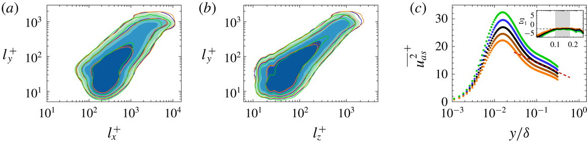
Superposition of the conditionally averaged turbulence intensity carried by the attached structures in
 $290<l_{y}^{+}<550$
: (a)
 $\overline{u_{as}^{2}}$
, (b)
 $\overline{w_{as}^{2}}$
and (c)
 $\overline{v_{as}^{2}}$
. The blue circles in (a) and (b) indicate
 $\unicode[STIX]{x1D6EF}_{1}=y\unicode[STIX]{x2202}\overline{u_{as}^{2}}/\unicode[STIX]{x2202}y$
and
 $\unicode[STIX]{x1D6EF}_{3}=y\unicode[STIX]{x2202}\overline{w_{as}^{2}}/\unicode[STIX]{x2202}y\overline{u_{as}^{2}}$
, which are the indicator functions of the logarithmic law, respectively. The inset shows a magnified view of the region where there is a plateau in the range
 $100<y^{+}<0.18\unicode[STIX]{x1D6FF}^{+}$
(shaded region). The red dashed lines in (a) and (b) correspond to
 $\overline{u_{as}^{2}}^{+}=7.3-3.010\ln (y/\unicode[STIX]{x1D6FF})$
and
 $\overline{w_{as}^{2}}=4.2-1.722\ln (y/\unicode[STIX]{x1D6FF})$
, respectively.

As mentioned earlier, it is worth highlighting that (4.1) does not correspond to the eddy intensity function at a given height of individual eddy. As shown in figure 7(a), the profiles of
 $\overline{u_{a}^{2}(y,l_{y})}$
exhibit the near-wall peak at
 $y^{+}\approx 15$
and their magnitudes increase with increasing
 $l_{y}$
. The eddy intensity functions proposed by Townsend (Reference Townsend1976) and Perry & Chong (Reference Perry and Chong1982) have no near-wall peak because the attached-eddy hypothesis assumed that the flow is inviscid (i.e. asymptotically high
 $Re_{\unicode[STIX]{x1D70F}}$
). Hence, the intensity functions are valid above the viscous dominant region and the near-wall peak is absent (see figure 21(a) in Perry & Chong (Reference Perry and Chong1982)). In addition, the magnitude of the eddy intensity function is constant regardless of hierarchical length scales. The value of their summation increases with the range of the length scales and thus the profile of the summation shows a logarithmic variation which is similar to the trend observed in
 $y^{+}>100$
in figure 7; see also figure 10(b) which shows the differences between
 $\overline{u_{a}^{2}}^{+}$
and the logarithmic variation. In other words, the profile of
 $\overline{u_{a}^{2}}^{+}$
represents the collective contribution of the attached
 $u$
structures with heights less than a given
 $l_{y}$
. One might think that this physical interpretation contradicts the inverse power-law PDF, since
 $l_{y}$
is consistent with the hierarchical length scale. Since the jitter and randomness of the discrete system or the continuous distribution of hierarchies lead to the inverse power-law PDF as discussed in Perry & Chong (Reference Perry and Chong1982), it is not surprising that the present attached structures follow
 $1/l_{y}$
; this concept is also related to the percolation behaviour of turbulent structures (§ 2).
To further examine the logarithmic behaviour in figure 7, we reconstruct the turbulence intensity through the superposition of over
 $290<l_{y}^{+}<550$
where the population density (
 $n_{s}$
) scales with
 $l_{y}$
in figure 6. Especially,
 $n_{s}$
of the attached
 $u$
is inversely proportional to
 $l_{y}$
. Here, the wall-normal profile of the reconstructed turbulence intensity (
 $\overline{u_{as,i}^{2}}$
) was computed by weighting the relative probability of the structures to the corresponding
 $\overline{u_{a,i}^{2}}$
:
 $$\begin{eqnarray}\overline{u_{as,i}^{2}}=\frac{\mathop{\sum }_{l_{y}}n_{s,i}(l_{y})\overline{u_{a,i}^{2}}(y,l_{y})}{\mathop{\sum }_{l_{y}}n_{s,i}(l_{y})}.\end{eqnarray}$$
Since
 $\overline{u_{a,i}^{2}}$
(4.1) indicates the turbulence intensities carried by representative structures at a given
 $l_{y}$
, their superposition (4.2) represents the turbulence intensities of the flow composed of these representative structures. The black dot in figure 8 shows the wall-normal variation of
 $\overline{u_{as,i}^{2}}$
. To confirm the logarithmic variations of
 $\overline{u_{as}^{2}}$
and
 $\overline{w_{as}^{2}}$
, the indicator function
 $$\begin{eqnarray}\unicode[STIX]{x1D6EF}_{i}(y)=y\unicode[STIX]{x2202}\overline{u_{as,i}^{2}}^{+}/\unicode[STIX]{x2202}y,\end{eqnarray}$$
which is constant in the logarithmic region, is also plotted in figure 8(a,b). For the wall-parallel components, a plateau appears over the same range
 $100<y^{+}<0.18\unicode[STIX]{x1D6FF}^{+}$
(see shaded region in the inset), verifying the presence of the logarithmic region formed by the attached structures. On the other hand, there is no clear constant region over
 $100<y^{+}<0.18\unicode[STIX]{x1D6FF}^{+}$
in the profile of
 $\overline{v_{as}^{2}}$
(figure 8
c). It is worth highlighting that we verify the logarithmic behaviour using the indicator function, which was absent in the experiments (Hultmark et al.
Reference Hultmark, Vallikivi, Bailey and Smits2012; Marusic et al.
Reference Marusic, Monty, Hultmark and Smits2013) on high-Reynolds-number flows due to the experimental uncertainty of the measurements. In addition, although the profile of the spanwise turbulence intensity exhibits the logarithmic variation, this behaviour is absent in the streamwise component at
 $Re_{\unicode[STIX]{x1D70F}}=2000$
in Jiménez & Hoyas (Reference Jiménez and Hoyas2008). They noted that the absence of the logarithmic variation is not only due to the viscous effect but is also due to the very long and wide motions (i.e. global modes or very-large-scale motions) since the behaviour of the streamwise turbulence intensity is much closer to the logarithmic variation after the removal of these motions. Given the fact that the profile of
 $\overline{u_{as}^{2}}$
is obtained among the structures with
 $290<l_{y}^{+}<550$
(i.e.
 $\overline{u_{as}^{2}}$
does not include the large-scale structures in the protrusions in figures 4 and 5), the present result supports this argument. Overall, the present results not only aid the attached-eddy hypothesis but also provide direct evidence for the presence of the attached structures, even in the moderate-Reynolds-number TBL.
5 Hierarchies of the attached structures
This section further explores the hierarchical nature of the attached structures, especially for the streamwise velocity fluctuations that exhibit the inverse power-law distribution (figure 6) as well as the self-similarity (figures 4 and 5) with respect to
 $l_{y}$
. In addition, long
 $u$
structures play an important role in wall turbulence because long negative-
 $u$
regions are associated with the net Reynolds shear force (Hwang, Lee and Sung Reference Hwang, Lee and Sung2016a
), and because the outer negative-
 $u$
structures extend to the wall and interact with near-wall streaks during the merging of the outer structures (Hwang et al.
Reference Hwang, Lee, Sung and Zaki2016b
).
5.1 Uniform momentum zones in the attached structures
As conjectured by Perry & Chong (Reference Perry and Chong1982), the attached eddies are in the form of hierarchies. Each hierarchy is composed of the eddies whose height grows from their initial roll-up height
 $(O(\unicode[STIX]{x1D708}/u_{\unicode[STIX]{x1D70F}}))$
to the height of the hierarchy (
 $l$
). Here, the height of the hierarchy corresponds to the height of the highest eddy within the hierarchy. In other words, there are several eddies whose heights are less than
 $l$
at a given hierarchy height
 $l$
and consequently the number of eddies or hierarchies increases with increasing
 $l$
. In addition, if we assume that the height of the highest hierarchy is the boundary layer thickness
 $\unicode[STIX]{x1D6FF}$
, the friction Reynolds number (
 $Re_{\unicode[STIX]{x1D70F}}=\unicode[STIX]{x1D6FF}u_{\unicode[STIX]{x1D70F}}/\unicode[STIX]{x1D708}$
) indicates the ratio of the highest hierarchy to the initial roll-up height. As a result, the number of eddies or hierarchies can be expected to increase with increasing
 $Re_{\unicode[STIX]{x1D70F}}$
. In this regard, De Silva, Hutchins & Marusic (Reference de Silva, Hutchins and Marusic2016) argued that a log–linear increase in the number of uniform momentum zones (UMZs) with increasing
 $Re_{\unicode[STIX]{x1D70F}}$
indicates a hierarchical length scale distribution. This interpretation was further supported by synthesizing the flow field using the attached-eddy model of Marusic (Reference Marusic2001). UMZs that contain roughly uniform streamwise velocity were first observed in the
 $x$
–
 $y$
plane of instantaneous flow fields by Meinhart & Adrian (Reference Meinhart and Adrian1995). In addition, UMZs commonly exist in multiple zones along the wall-normal direction (Adrian et al.
Reference Adrian, Meinhart and Tomkins2000), implying the hierarchical nature. To further examine the hierarchical characteristics of the attached
 $u$
structures, we examine the instantaneous streamwise velocity (
 $U$
) within these objects.
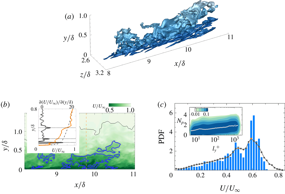
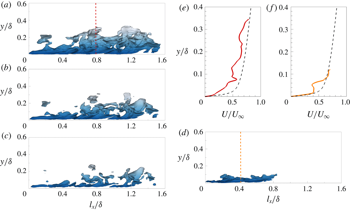
Figure 9(a) shows an attached structure of negative
 $u$
(that enclosed by the black box in figure 3
a) and a streamwise slice at
 $z/\unicode[STIX]{x1D6FF}=2.86$
is illustrated in figure 9(b). This structure extends from the wall to
 $y\approx 0.8\unicode[STIX]{x1D6FF}$
and in particular, the profile of
 $U$
at
 $x/\unicode[STIX]{x1D6FF}=9.77$
(see the inset in figure 9
b) shows several jumps in velocity across the structure (as indicated by the dotted horizontal lines), separating zones of roughly uniform
 $U$
; low
 $\unicode[STIX]{x2202}U/\unicode[STIX]{x2202}y$
(orange line) also appears within the UMZs. Given that the UMZs produce the local maxima in the histogram of
 $U$
(Adrian et al.
Reference Adrian, Meinhart and Tomkins2000), we plot the histogram of
 $U$
in the cross-stream plane of the identified structures at
 $x/\unicode[STIX]{x1D6FF}=9.77$
in figure 9(c). Although there are several local maxima, the two at
 $U/U_{\infty }\approx 0.5$
and 0.6, which are the consequence of UMZs, are preserved when the data are accumulated over the entire structure (grey line). To further examine the number of UMZs in the attached structures, the joint PDF of the height (
 $l_{y}$
) and the number of local maxima (
 $N_{p}$
) is shown in the inset of figure 9(c). Here, the inserted dots indicate the mean
 $N_{p}$
at a given
 $l_{y}$
. The number of UMZs in each structure increases with increasing
 $l_{y}$
, which confirms the hierarchical nature of the identified structures (De Silva et al.
Reference de Silva, Hutchins and Marusic2016). In other words,
 $l_{y}$
could be consistent with the hierarchy length scale in connection with the results in § 3.
(a) A sample attached structure of negative
 $u$
(that enclosed by the black box in figure 3
a). (b) Contour of the instantaneous streamwise velocity (
 $U$
) in the
 $x$
–
 $y$
plane at
 $z/\unicode[STIX]{x1D6FF}=2.86$
. The blue line is a slice of the object shown in (a). The black line indicates the instantaneous TNTI. The inset shows a comparison of the instantaneous (orange line) and mean (dashed line) streamwise velocity profiles at
 $x/\unicode[STIX]{x1D6FF}=9.77$
(indicated by the vertical dashed line in the contour). The grey line represents
 $\unicode[STIX]{x2202}U/\unicode[STIX]{x2202}y$
, except the region for
 $y^{+}<50$
due to the strong shear close to the wall. The horizontal dotted lines indicate step-like jumps of
 $U$
across the structure, which separate the zones of roughly constant
 $U$
. (c) Histogram of
 $U$
in the cross-stream plane of the identified object at
 $x/\unicode[STIX]{x1D6FF}=9.77$
, which contains the two distinct local maxima (at
 $U/U_{\infty }\approx 0.5$
and 0.6) that are associated with possible uniform momentum zones (UMZs). The grey line shows the PDF of
 $U$
within the identified object and the orange circles denote the local maxima. The inset shows the joint PDF of the height (
 $l_{y}$
) and the number of UMZs (
 $N_{p}$
). The inserted dots indicate the mean
 $N_{p}$
with respect to
 $l_{y}$
. The contour levels are logarithmically distributed.

(a) Variation of the near peak magnitude of
 $\overline{u_{a}^{2}}^{+}(\overline{u_{a,max}^{2}}^{+})$
with respect to
 $l_{y}^{+}$
. The orange line shows
 $\overline{u_{a,\max }^{2}}^{+}\sim 0.66\ln (l_{y}^{+})$
over
 $100<l_{y}^{+}<550$
. (b)
 $\overline{u_{a}^{2}}^{+}-\{-3.010\ln (y/\unicode[STIX]{x1D6FF})\}$
for the attached
 $u$
structures within
 $100<l_{y}^{+}<750$
.
 $l_{y}$
are logarithmically distributed. The solid lines indicate the structures with
 $l_{y}^{+}=150$
, 190, 240, 300 and 400 and the vertical dashed lines represent the logarithmic region (
 $100<y^{+}<0.18\unicode[STIX]{x1D6FF}^{+}$
).

In this work, we analyse the number of UMZs within the attached structures of
 $u$
. At a single Reynolds number (i.e.
 $Re_{\unicode[STIX]{x1D70F}}=980$
), the number of UMZs increases logarithmically with increasing
 $l_{y}$
(figure 9), which directly indicates the relationship between the multiple UMZ phenomena (Meinhart & Adrian Reference Meinhart and Adrian1995; Adrian et al.
Reference Adrian, Meinhart and Tomkins2000) and the hierarchical distribution of the attached structures of
 $u$
. Hence, one attached structure of
 $u$
might be consistent with multiple hairpin packets of various ages and sizes since small packets can be covered by larger packets that convect faster than the smaller ones (Adrian et al.
Reference Adrian, Meinhart and Tomkins2000); note that the inclination angle of the
 $u$
structures ranges from
 $8.8^{\circ }$
to
 $16^{\circ }$
, which is similar to that of hairpin packets. In addition, given that the wake of attached vortex clusters identified in del Álamo et al. (Reference del Álamo, Jiménez, Zandonade and Moser2006) is associated with multiple UMZs, the attached structures of
 $u$
might be shrouded in the vortex clusters. However, we need to perform a more extensive examination of the three-dimensional vortices surrounding the
 $u$
structures.
One could question our method for the detection of UMZs within the
 $u$
structures: are the local maxima observed in the histogram (figure 9
c) due to the conditional sampling of
 $U$
in a selective volume? As first observed by Meinhart & Adrian (Reference Meinhart and Adrian1995), the phenomenon of roughly constant uniform momentum in the
 $x$
–
 $y$
plane of instantaneous flow fields is a local event that is random and time-varying. In order to quantify the UMZs, Adrian et al. (Reference Adrian, Meinhart and Tomkins2000) analysed the histogram of
 $U$
with a streamwise domain length of 2000 wall units. De Silva et al. (Reference de Silva, Hutchins and Marusic2016) also used the similar length to detect the UMZs. In other words, these previous studies sampled
 $U$
selectively in the short streamwise domain at a certain spanwise location. As discussed in Adrian et al. (Reference Adrian, Meinhart and Tomkins2000), the local maxima in the histogram depend on the time averaging and the streamwise length of the data. This behaviour was discussed in Kwon et al. (Reference Kwon, Philip, de Silva, Hutchins and Monty2014), who examined the variation in the local maxima as a function of the streamwise domain length; when the streamwise domain increases up to
 $6h$
(where
 $h$
is the channel half-height), several peaks disappear and only one peak survives. To overcome this limitation, the edges of the UMZs must be carefully identified. In the present work, we defined the boundary of the UMZs by examining the three-dimensional
 $u$
structures. As a result, the histogram of
 $U$
obtained as a function of the height of each
 $u$
structure shows several maxima even when the streamwise length of the structures increases (figure 9
c). The negative-
 $u$
regions in the two-dimensional plane represent the UMZs induced by surrounding vortices (Ganapathisubramani, Longmire & Marusic Reference Ganapathisubramani, Longmire and Marusic2003; Tomkins & Adrian Reference Tomkins and Adrian2003; Hutchins, Hambleton & Marusic Reference Hutchins, Hambleton and Marusic2005). Retrograde vortices can exist on the shear layer of positive-
 $u$
structures (Ganapathisubramani et al.
Reference Ganapathisubramani, Hutchins, Monty, Chung and Marusic2012), which may induce the roughly uniform momentum greater than the mean velocity. In this respect, sampling the streamwise velocity within the
 $u$
structures is an appropriate method for the detection of UMZs in three-dimensional flow fields.
It is worth highlighting the importance of UMZs in the context of the attached-eddy hypothesis. The work of Meinhart & Adrian (Reference Meinhart and Adrian1995) not only demonstrated the general existence of UMZs but also contained that UMZs are connections between the discrete system and the continuous system (Perry & Chong Reference Perry and Chong1982). Meinhart & Adrian (Reference Meinhart and Adrian1995) used the term ‘zones’ to emphasize that the step-like jumps in
 $U$
are instantaneous phenomena, in contrast to ‘layers’ such as the buffer layer and logarithmic layer, which are defined in terms of the mean quantities (Adrian et al.
Reference Adrian, Meinhart and Tomkins2000, § 5.3), and concluded that ‘The zonal structure reported here offers some new ways of conceptualizing the structure of wall turbulence. The conventional decomposition of the boundary layer into a wall layer, a logarithmic layer and a wake region is based on time-averaged properties of regions of fixed vertical dimension. The zones, in contrast, are instantaneous, time-evolving entities, whose characteristics contribute to the mean properties of each of the convection layers.’ In this regard, UMZs are strong evidence for describing the continuous system (Perry & Chong Reference Perry and Chong1982), which is a result of the randomness in the discrete system. Perry & Chong (Reference Perry and Chong1982) assumed that quantum-jump phenomena in the discrete system are smoothed by the randomness and jitter of turbulence, which leads to the inverse power-law PDF of the hierarchy length scale in the continuous system. The present findings show directly that the attached
 $u$
structures composed of multiple UMZs follow the hierarchical length scale distribution (figure 9) and contribute to the formation of the logarithmic region (figure 8).
5.2 Near-wall peaks of the streamwise turbulence intensity
The logarithmic variation of the streamwise turbulence intensity (1.2) implies that the magnitude of
 $\overline{u^{2}}^{+}$
at a fixed
 $y^{+}$
is proportional to
 $\ln (Re_{\unicode[STIX]{x1D70F}})$
(Jiménez & Hoyas Reference Jiménez and Hoyas2008; Jiménez Reference Jiménez2012; Marusic et al.
Reference Marusic, Baars and Hutchins2017); the near-wall peak
 $\overline{u_{max}^{2}}^{+}$
, which appears at
 $y^{+}\approx 15$
, exhibits
 $\overline{u_{max}^{2}}^{+}\sim \ln (Re_{\unicode[STIX]{x1D70F}})$
. This behaviour was first reported experimentally in DeGraaff & Eaton (Reference DeGraaff and Eaton2000) and they suggested a mixed scaling (i.e.
 $u_{\unicode[STIX]{x1D70F}}$
and
 $U_{\infty }$
) for
 $\overline{u_{max}^{2}}^{+}$
in the context of the attached-eddy hypothesis. Subsequently, several experimental and numerical works reported the logarithmic increase of
 $\overline{u_{max}^{2}}^{+}$
(Marusic & Kunkel Reference Marusic and Kunkel2003; Hoyas and Jiménez Reference Hoyas and Jiménez2006; Sillero, Jiménez & Moser Reference Sillero, Jiménez and Moser2013; Lee & Moser Reference Lee and Moser2015; Ahn et al.
Reference Ahn, Lee, Lee, Kang and Sung2015, Örlü et al.
Reference Örlü, Fiorini, Segalini, Bellani, Talamelli and Alfredsson2017). At extremely high Reynolds numbers (
 $Re_{\unicode[STIX]{x1D70F}}>30\,000$
), some studies (Hultmark et al.
Reference Hultmark, Vallikivi, Bailey and Smits2012; Vallikivi et al.
Reference Vallikivi, Ganapathisubramani and Smits2015) found that the growth of inner peak is absent, but these results might be due to spatial and temporal resolution issues (Sillero et al.
Reference Sillero, Jiménez and Moser2013; Marusic et al.
Reference Marusic, Baars and Hutchins2017). Given that the behaviour
 $\overline{u_{max}^{2}}^{+}\sim \ln (Re_{\unicode[STIX]{x1D70F}})$
can be explained with Townsend’s attached-eddy hypothesis, we further examine the variation in the near-wall peak of
 $\overline{u_{a}^{2}}^{+}$
with
 $l_{y}$
(figure 7) because
 $l_{y}$
is associated with the hierarchy length scale.
As pointed out in figure 7, the profiles of
 $\overline{u_{a}^{2}}^{+}$
have a near-wall peak and its magnitude increases with increasing
 $l_{y}$
. Figure 10(a) shows the variations of the peak
 $\overline{u_{a}^{2}}^{+}$
according to
 $l_{y}^{+}$
. As seen, there is a logarithmic increase in the magnitude of the peak
 $\overline{u_{a}^{2}}^{+}$
with increasing
 $l_{y}^{+}$
in
 $100<l_{y}^{+}<550$
with a slope of 0.66. This result is in good agreement with the results for the slope of the increase in the magnitude of the peak
 $\overline{u^{2}}$
versus
 $Re_{\unicode[STIX]{x1D70F}}$
obtained in recent DNSs 0.65 (Sillero et al.
Reference Sillero, Jiménez and Moser2013) and in experiments 0.63 (Marusic et al.
Reference Marusic, Baars and Hutchins2017); for the DNS dataset of turbulent channel flows up to
 $Re_{\unicode[STIX]{x1D70F}}=5200$
, the slope is 0.642 (Lee & Moser Reference Lee and Moser2015). Sillero et al. (Reference Sillero, Jiménez and Moser2013) and Marusic et al. (Reference Marusic, Baars and Hutchins2017) noted that this value is approximately half of
 $A_{1}$
(i.e. the slope of the logarithmic term in 1.2a) since the lower bound of the logarithmic region scales with
 $Re_{\unicode[STIX]{x1D70F}}^{0.5}$
in contrast to the classical scaling (e.g.
 $O(100\unicode[STIX]{x1D708}/u_{\unicode[STIX]{x1D70F}})$
) in Perry & Chong (Reference Perry and Chong1982). As discussed in § 4, the profile of
 $\overline{u_{a}^{2}}^{+}$
is the result of the conditional averaging of the intense
 $u$
within the identified structures (
 $|u|>\unicode[STIX]{x1D6FC}u_{rms}$
), leading to the difference in
 $A_{1}$
; the magnitude of
 $A_{1}$
for
 $\overline{u_{a}^{2}}^{+}$
is larger than that for
 $\overline{u^{2}}$
(
 $A_{1}=1.26$
in Marusic et al.
Reference Marusic, Monty, Hultmark and Smits2013. However, the slope of the variation in the magnitude of the peak
 $\overline{u_{a}^{2}}^{+}$
is similar to that of the variation in the total turbulence intensity, representing that the attached structures of
 $u$
could play a dominant role in the increase of the near-wall peak for the total turbulence intensity. At the present Reynolds number, the attached structures contribute 20–35 % of
 $\overline{u^{2}}$
at
 $y<0.3\unicode[STIX]{x1D6FF}$
, while the contribution of the other components (i.e. detached structures and weak turbulence (
 $|u|<\unicode[STIX]{x1D6FC}u_{rms}$
)) is 75–80 % leading to the absence of the logarithmic behaviour in
 $\overline{u^{2}}$
over
 $100<y^{+}<0.18\unicode[STIX]{x1D6FF}^{+}$
. In addition, it would be instructive to examine the Reynolds-number dependence of the lower bound of the logarithmic region for
 $\overline{u_{a}^{2}}$
, which is consistent with the onset of the self-similarity in figures 4 and 5 (i.e.
 $l_{y}^{+}=100\approx 3Re_{\unicode[STIX]{x1D70F}}^{0.5}$
in the present data), but this task is beyond the scope of the present work.
To further support the upward shift of the profiles in figure 7(a), we subtract the logarithmic function (i.e.
 $-3.010\ln (y/\unicode[STIX]{x1D6FF})$
) from (4.1) in figure 10(b). As seen, there is a region where the difference between
 $\overline{u_{a}^{2}}$
and
 $-3.010\ln (y/\unicode[STIX]{x1D6FF})$
is constant and the difference increases with increasing
 $l_{y}$
. This trend also reflects the collective contribution of the attached
 $u$
structures with heights less than a given
 $l_{y}$
. The results in figure 10(b) indicate that the slope of each
 $\overline{u_{a}^{2}}$
is close to
 $-3.010$
and their logarithmic variations shift upwards with increasing
 $l_{y}$
, representing that the additive constant in (1.2) would depend on the Reynolds number; similar behaviour was also reported in Jiménez & Hoyas (Reference Jiménez and Hoyas2008) by assessing the turbulence intensity data over a wide range of
 $Re_{\unicode[STIX]{x1D70F}}$
. Note that the range of the logarithmic behaviour is small in the present work due to the Reynolds number (
 $Re_{\unicode[STIX]{x1D70F}}\approx 10^{3}$
). It would be valuable to examine this trend at high
 $Re_{\unicode[STIX]{x1D70F}}$
(i.e. increase the range of
 $l_{y}$
).
5.3 Nested hierarchies
As discussed earlier, attached
 $u$
structures with a given
 $l_{y}$
represent the collective contributions of the structures with heights less than
 $l_{y}$
. In addition, these structures are composed of multiple uniform momentum zones (UMZs). The combination of these two results demonstrates the concept of nested hierarchies proposed by Adrian et al. (Reference Adrian, Meinhart and Tomkins2000). They suggested that small packets (or UMZs) exist within larger packets due to the difference in their convection velocities. The smaller packet contained within the larger one induces the lower streamwise momentum (i.e. strong retardation of
 $U$
). Adrian et al. (Reference Adrian, Meinhart and Tomkins2000) described such flow patterns as a nested hierarchy which leads to the presence multiple UMZs; see Adrian et al. (Reference Adrian, Meinhart and Tomkins2000, figure 22). Interestingly, the regions of different streamwise momentum are depicted in a closed loop even though a certain level of
 $U$
(i.e. interfaces of UMZs) extends from the left edge to the right edge of the flow field. This schematic representation resembles the flow patterns associated with attached
 $u$
structures.
Figure 11(a,d) shows a side view of sample attached
 $u$
structures with
 $l_{y}=0.33\unicode[STIX]{x1D6FF}$
and
 $l_{y}=0.12\unicode[STIX]{x1D6FF}$
, respectively. As seen, the streamwise length of the shorter structure in figure 11(d) is
 $l_{x}=0.8\unicode[STIX]{x1D6FF}$
which is approximately half of the larger structure in figure 11(a). As
 $\unicode[STIX]{x1D6FC}$
increases, the size of the structure in figure 11(a) shrinks and is split into smaller structures that are attached and detached objects with intense
 $u$
in figure 11(b,c). The structures in figure 11(c) are nested within the region of
 $-2.2u_{rms}<u<-1.5u_{rms}$
. In other words, a larger structure (or a higher hierarchy) contains several smaller structures (or shorter hierarchies less than a given
 $l_{y}$
) with intense
 $u$
. In particular, the split structure close to the wall (
 $0<l_{x}/\unicode[STIX]{x1D6FF}<0.8$
) is similar to the shorter structure identified at
 $\unicode[STIX]{x1D6FC}=1.5$
in figure 11(d). This is evident when we compare the wall-normal variations of
 $U$
. Figure 11(e,f) shows the wall-normal profiles of
 $U$
at the positions (
 $l_{x}/\unicode[STIX]{x1D6FF}=0.5$
and
 $l_{z}/\unicode[STIX]{x1D6FF}=0.5$
) denoted by the vertical dashed lines in (a) and (d). As seen, the profile of the larger structure (figure 11
e) exhibits several velocity jumps (at least more than two UMZs) across the wall-normal direction whereas that of the shorter one (figure 11
f) shows one UMZ. In addition, the velocity deficit is more evident in figure 11(e); the dashed line indicates the wall-normal profiles of the mean streamwise velocity. At
 $y/\unicode[STIX]{x1D6FF}<0.03$
, in particular, the magnitude of
 $U$
in figure 11(f) is similar to that of the mean streamwise velocity whereas
 $U$
in figure 11(e) shows the larger velocity deficit. This behaviour indicates that one attached structure of
 $u$
with
 $l_{y}$
is the collective contributions of the shorter structures (
 ${<}l_{y}$
) since intense
 $u$
regions (figure 11
b,c) belong to the taller one (figure 11
a). Recently, Laskari et al. (Reference Laskari, de Kat, Hearst and Ganapathisubramani2018) showed that the increase in the number of UMZs results in a strong retardation of
 $U$
close to the wall because additional UMZs (i.e. additional momentum deficit) are observed in the near-wall region. This is similar to the result in the present work that taller structures of
 $u$
have strong momentum deficit close to the wall leading to the increase of the near-wall peak of
 $\overline{u_{a}^{2}}$
with
 $l_{y}$
. Based on the mean streamwise and wall-normal velocities associated with UMZs, Laskari et al. (Reference Laskari, de Kat, Hearst and Ganapathisubramani2018) reported that a high number of UMZs is associated with large-scale structures of ejections. Given that the attached structures of negative
 $u$
can contain the ejection event (
 $u<0$
and
 $v>0$
), this phenomenon can be explained in the context of nested hierarchies. Note that a low number of UMZs exhibits the sweep event (
 $u$
 ${>}$
0 and
 $v<0$
) which is associated with the attached structures of positive
 $u$
in the present work. This may indicate that the number of UMZs is relatively small in the positive-
 $u$
structures compared to that in the negative-
 $u$
objects at a given
 $l_{y}$
. In future efforts, it would be valuable to explore the attached structures of negative and positive
 $u$
and examine their hierarchical nature related to multiple UMZs.
6 Conclusions
We have demonstrated for the first time that the wall-attached structures of
 $u$
are energy-containing motions satisfying the attached-eddy hypothesis (Townsend Reference Townsend1976), not only because they are self-similar to
 $l_{y}$
, but also because there are two strong pieces of evidence: (i) the inverse power-law PDF, and (ii) the logarithmic variation of the streamwise turbulence intensity (
 $\overline{u_{a}^{2}}$
) carried by the identified structures. In particular, we show the presence of the logarithmic region by reconstructing the intensity profile from the superposition of the wall-attached structures in spite of the absence of the logarithmic behaviour in the total turbulence intensity at the present Reynolds number (
 $Re_{\unicode[STIX]{x1D70F}}\approx 1000$
). In addition, the wall-attached structures of the cross-stream components (
 $w$
and
 $v$
) exhibit the self-similarity with respect to
 $l_{y}$
. Although their lengths are relatively shorter than that of
 $u$
, the widths of all the
 $u_{i}$
structures are comparable and linearly proportional to
 $l_{y}$
over a broad range, indicating the presence of tall vortical structures. In addition, the spanwise turbulence intensity contained within the attached structures of
 $w$
follows the logarithmic variation over the same range of the streamwise component (
 $100<y^{+}<0.18\unicode[STIX]{x1D6FF}^{+}$
). We further explore the hierarchical nature of the attached
 $u$
structures that exhibit the hierarchical length scale distribution (PDF
 $l_{y}^{-1}$
). The wall-normal profile of the instantaneous streamwise velocity within the attached
 $u$
structures shows step-like jumps, reminiscent of UMZs; in particular the number of UMZs within the objects increases with increasing
 $l_{y}$
, representing that the structures of
 $u$
are composed of multiple UMZs (or nested hierarchies in a sense of hairpin packet paradigm). Furthermore, the magnitudes of
 $\overline{u_{a}^{2}}$
increase with increasing
 $l_{y}$
, and especially those of the near-wall peak are proportional to
 $\ln (l_{y}^{+})$
. These results indicate that
 $\overline{u_{a}^{2}}$
is made up of the collective contribution of the attached
 $u$
structures with heights less than a given
 $l_{y}$
. Although we have identified the attached structures in a TBL for only a single Reynolds number, their hierarchical features ensure that they will also be present in high-Reynolds-number flows. We anticipate that examining the Reynolds-number effects on attached structures will improve the predictive model (Marusic, Mathis & Hutchins Reference Marusic, Mathis and Hutchins2010) and that exploring their dynamics will facilitate deeper insights into the multiscale energy cascade of wall turbulence.
(a–d) Side view of isosurfaces of the attached
 $u$
structures (
 $u=-\unicode[STIX]{x1D6FC}u_{rms}$
). (a) A sample attached structure of
 $u$
(
 $\unicode[STIX]{x1D6FC}=1.5$
) with
 $l_{y}=0.33\unicode[STIX]{x1D6FF}$
. (b,c) Isosurfaces of the structure in (a) at higher thresholds;
 $\unicode[STIX]{x1D6FC}=1.9$
(b) and 2.2 (c). (d) A sample attached structure of
 $u$
(
 $\unicode[STIX]{x1D6FC}=1.5$
) with
 $l_{y}=0.12\unicode[STIX]{x1D6FF}$
. (e,f) Wall-normal profiles of
 $U$
for the structures in (a) and (d) obtained at
 $l_{x}/\unicode[STIX]{x1D6FF}=0.5$
and
 $l_{z}/\unicode[STIX]{x1D6FF}=0.5$
(denoted by vertical dashed lines in (a,d). The dashed line represents the mean streamwise velocity.
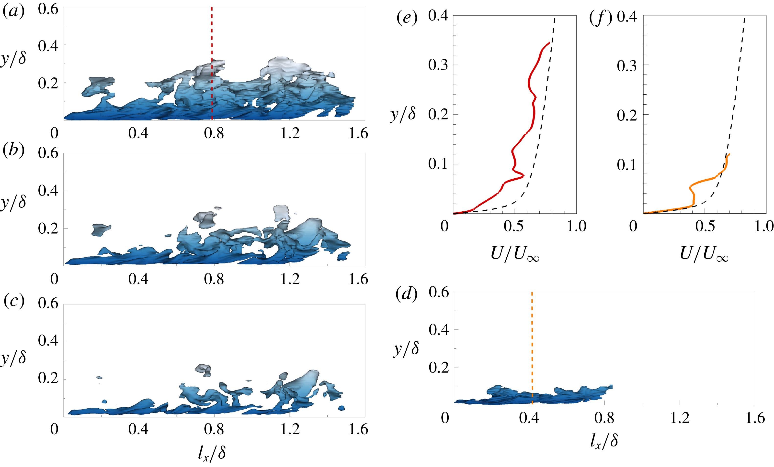
Acknowledgements
This work was supported by the National Research Foundation of Korea (no. 2018001483), the Supercomputing Centre (KISTI) and the KUSTAR-KAIST institute.
Appendix A. Effects of the structure-identification threshold
To address the influence of the threshold value
 $\unicode[STIX]{x1D6FC}$
, we plot the population density, size distributions and reconstructed turbulence intensity over a range of thresholds from 1.4 to 1.7 where the percolation transition occurs (figure 2
a). Here, we only include the results of the
 $u$
clusters to avoid any repetition. Figure 12 shows the threshold effect on the population density of clusters according to
 $y_{min}$
and
 $y_{max}$
. Regardless of
 $\unicode[STIX]{x1D6FC}$
, two distinct regions are observed: the wall-attached and detached groups. As discussed in § 2, there is a weak peak at
 $y_{min}^{+}\approx 7$
and
 $y_{max}^{+}\approx 50$
. The structures in the vicinity of this peak can be the fragments of large attached structures or objects that are developing into larger objects. Figure 13(a,b) illustrates the distribution of the sizes of the attached structures by varying
 $\unicode[STIX]{x1D6FC}$
. The contour lines collapse well, indicating that the self-similarity of the structures with respect to their height (
 $l_{y}$
) is conserved. Figure 13(c) represents the threshold effect on the logarithmic behaviour of the reconstructed streamwise turbulence intensity
 $\overline{u_{as}^{2}}^{+}$
. Although the profile of
 $\overline{u_{as}^{2}}^{+}$
shifts upwards with increasing
 $\unicode[STIX]{x1D6FC}$
, the logarithmic variation is observed with a similar slope at each
 $\unicode[STIX]{x1D6FC}$
. In the inset, it is evident that the indicator function (
 $\unicode[STIX]{x1D6EF}_{1}$
) has a constant value over the region
 $100<y^{+}<0.18\unicode[STIX]{x1D6FF}^{+}$
(shaded region).
The percolation threshold effect on the number of
 $u$
clusters per unit wall-parallel area as a function of
 $y_{min}$
and
 $y_{max}$
. The colour contour is consistent with that in figure 2(b). The line contour is 0.0016 when
 $\unicode[STIX]{x1D6FC}=1.3$
(orange), 1.4 (brown), 1.5 (black), 1.6 (blue) and 1.7 (green).

(a,b) Joint PDFs of the logarithms of the sizes (
 $l_{x}$
and
 $l_{z}$
) of the attached structures and of the height (
 $l_{y}$
). The colour contour is consistent with that in figures 4 and 5. The line contour is 0.004, 0.04 and 0.4 with varying
 $\unicode[STIX]{x1D6FC}$
. (c) Wall-normal variation of
 $\overline{u_{as}^{2}}^{+}$
with varying
 $\unicode[STIX]{x1D6FC}$
:
 $\unicode[STIX]{x1D6FC}=1.3$
(orange), 1.4 (brown), 1.5 (black), 1.6 (blue) and 1.7 (green). The red dashed line indicates the logarithmic variation. The inset shows the corresponding indicator function
 $\unicode[STIX]{x1D6EF}_{1}$
.