1. Introduction
Vortices can be subjected to many instabilities in stably stratified and rotating fluids because of their own structure or because of interactions with other vortices. If we exclude the latter possibility by restricting the problem to the idealized configuration of a single vertical columnar axisymmetric vortex, there are still several instability mechanisms that can disrupt a vortex. The shear and centrifugal instabilities are not specific to a stratified-rotating fluid and have been well-known since Rayleigh (Reference Rayleigh1880, Reference Rayleigh1917). The former is a two-dimensional instability that can destabilize non-axisymmetric perturbations with azimuthal wavenumbers
 $m\geqslant 2$
if the vertical vorticity derivative
 ${\it\zeta}^{\prime }(r)$
vanishes for some radius
 $r$
(Rayleigh Reference Rayleigh1880; Howard & Gupta Reference Howard and Gupta1962; Carton & McWilliams Reference Carton, McWilliams, Nihoul and Jamart1989; Carnevale & Kloosterziel Reference Carnevale and Kloosterziel1994). This necessary condition is equivalent to the inflection point condition for parallel shear flows. The centrifugal instability is intrinsically three-dimensional and most unstable for short axial wavelength and axisymmetric perturbations
 $m=0$
in inviscid fluids. The classical Rayleigh criterion (Rayleigh Reference Rayleigh1917) for the centrifugal instability can be extended to stratified-rotating inviscid fluid (Kloosterziel & van Heijst Reference Kloosterziel and van Heijst1991; Billant & Gallaire Reference Billant and Gallaire2005) by replacing the circulation by the absolute circulation, i.e. a necessary and sufficient instability condition is that the square of the absolute circulation decreases for increasing radius, regardless of the stratification. Even if the axisymmetric mode is dominant in an inviscid fluid, it should be noted that non-axisymmetric modes can be the most unstable in viscous fluids owing to the combined effects of stratification and viscosity (Billant, Colette & Chomaz Reference Billant, Colette and Chomaz2004) or confinement in shallow layers (Lahaye & Zeitlin Reference Lahaye and Zeitlin2015) which damp short axial wavelengths.
Recently, a different type of instability has been shown to occur specifically in vortices in a stratified rotating fluid: the radiative instability (Smyth & McWilliams Reference Smyth and McWilliams1998; Schecter & Montgomery Reference Schecter and Montgomery2004; Billant & Le Dizès Reference Billant and Le Dizès2009; Le Dizès & Billant Reference Le Dizès and Billant2009; Riedinger, Le Dizès & Meunier Reference Riedinger, Le Dizès and Meunier2010, Reference Riedinger, Le Dizès and Meunier2011; Park & Billant Reference Park and Billant2012, Reference Park and Billant2013). This instability is due to a coupling between the waves sustained by the vortex and inertial-gravity waves in the surrounding fluid. The mechanism of the instability can be interpreted as a wave over-reflection at the critical radius where the azimuthal phase velocity matches the angular velocity of the base flow, a radius which exists only for non-axisymmetric waves. The radiative instability is most unstable when the fluid is strongly stratified and non-rotating. As the background rotation increases, its growth rate decreases and vanishes in the quasi-geostrophic limit (strongly stratified and rapidly rotating fluid). This regime pertains to large scale atmospheric and oceanic vortices (see Schecter & Montgomery (Reference Schecter and Montgomery2006) for a summary of the typical characteristics of various geophysical vortices).
A fourth type of instability has been evidenced by Gent & McWilliams (Reference Gent and McWilliams1986) on vortices with zero-circulation in quasi-geostrophic fluids. In contrast to the shear or centrifugal instabilities, it is most unstable for a finite axial wavenumber and occurs only for the azimuthal wavenumber
 $m=1$
. This instability bends and fragments the vortex into lenticular vortices (Gent & McWilliams Reference Gent and McWilliams1986; Hua Reference Hua1998; Smyth & McWilliams Reference Smyth and McWilliams1998). Gent & McWilliams (Reference Gent and McWilliams1986) called this three-dimensional instability the ‘internal instability’ as opposed to the ‘external instability’, i.e. the two-dimensional shear instability. Here, we shall call the internal instability the ‘Gent–McWilliams instability’ in order to distinguish it from the other types of three-dimensional instability. The Gent–McWilliams (GMW) instability is the most dangerous instability in quasi-geostrophic fluids for sufficiently steep vortex profiles such as for example the Carton & McWilliams (Reference Carton, McWilliams, Nihoul and Jamart1989) vortex (Gaussian angular velocity profile). Even if the instability is three-dimensional, Gent & McWilliams (Reference Gent and McWilliams1986) have also shown that the necessary conditions for the shear instability (Rayleigh and Fjortoft’s criteria) also apply to the GMW instability in a quasi-geostrophic fluid.
Flierl (Reference Flierl1988) has shown that the GMW instability also occurs on vortices with a piecewise profile with two levels of non-zero uniform vorticity in quasi-geostrophic fluids. A necessary condition for instability is that
 $({\it\zeta}_{i}-{\it\zeta}_{o}){\it\zeta}_{o}<0$
, where
 ${\it\zeta}_{i}$
and
 ${\it\zeta}_{o}$
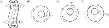
are the inner and outer vorticities. This is equivalent to the condition that the vorticity gradient changes sign between the two vorticity jumps. When the vortices are isolated (i.e. zero circulation), the GMW instability is of a long-wavelength nature, i.e. its growth rate is positive as soon as the axial wavenumber is non-zero. In contrast, only finite axial wavenumbers (i.e. wavenumbers above a non-zero wavenumber cutoff) are unstable when the circulation is non-zero. Flierl (Reference Flierl1988) has also provided a simple explanation of the instability mechanism. Two different processes are involved: self-induced motion when the vortex is slightly bent along the vertical, and two-dimensional advection by the vorticity anomalies generated when the two vorticity contours are shifted relative to each other. This mechanism is illustrated in figure 1 and explained in detail in the caption.
Mechanism of the GMW instability as explained by Flierl (Reference Flierl1988) for piecewise vortex profiles in a quasi-geostrophic fluid. As sketched in (a), we consider a columnar vortex with two levels of constant vorticity which is perturbed by a long-wavelength bending perturbation. The solid and dotted lines show the perturbed and unperturbed vorticity contours, respectively. The vorticity is assumed positive in the core region and negative in the surrounding annulus. The vorticity contours in the horizontal cross-section A are represented in (b). The initial displacements of the inner and outer contours are chosen to be in the positive
 $x$
direction and equal (
 ${\rm\Delta}x_{1}={\rm\Delta}x_{2}>0$
). Because of self-induction, the bent vortex will then rotate in the positive sense about its unperturbed position. As indicated in (c), this leads to displacements in the positive
 $y$
direction (
 ${\rm\Delta}y_{1}>0$
,
 ${\rm\Delta}y_{2}>0$
) in the cross-section A. However, the two contours are not displaced by the same amount: the inner contour turns out to be more displaced than the outer one (
 ${\rm\Delta}y_{1}>{\rm\Delta}y_{2}>0$
). In turn, since the vorticity is not of the same sign in the inner and outer regions, this differential displacement creates positive (
 $\oplus$
) and negative (
 $\ominus$
) vorticity anomalies. As sketched in (d), this dipole of vorticity anomalies tends to further translate the vortex in the positive
 $x$
direction, i.e. in the same direction as the initial displacement. The same reasoning can be applied to the motions in the cross-section B. There is therefore a positive feedback which will make the initial bending perturbation grow.

Smyth & McWilliams (Reference Smyth and McWilliams1998) have studied the stability of the Carton and McWilliams vortex beyond the quasi-geostrophic regime. Most interestingly, they have shown that the GMW instability exists only in presence of both stratification and rotation. However, this observation remains unexplained. The Rayleigh and Fjortoft’s stability criteria (Gent & McWilliams Reference Gent and McWilliams1986) indeed apply only to quasi-geostrophic fluids.
Hence, the main questions that we would like to address in this paper are: why does the GMW instability occur only in stratified rotating fluids? And is it possible to derive an instability condition valid for arbitrary rotation and stratification? These questions are intimately linked to the preliminary question: what is the general mechanism of the GMW instability? Even if a mechanism has been highlighted by Flierl (Reference Flierl1988) for piecewise vorticity profiles in quasi-geostrophic fluids, it is not straightforward to extend it to arbitrary rotation and stratification and/or to continuous vorticity profiles.
Interestingly, Reasor & Montgomery (Reference Reasor and Montgomery2001) and Reasor, Montgomery & Grasso (Reference Reasor, Montgomery and Grasso2004) have shown that certain vortices in quasi-geostrophic fluids tend to align when they are tilted, i.e. a behaviour opposite to the GMW instability. This alignment process has been attributed to a critical layer damping of the bending mode when
 ${\it\zeta}^{\prime }(r_{c})<0$
, where
 $r_{c}$
is the critical radius where the phase velocity of the wave
 ${\it\omega}/m$
is equal to the angular velocity of the vortex
 ${\it\Omega}(r_{c})$
(Briggs, Daugherty & Levy Reference Briggs, Daugherty and Levy1970; Schecter, Montgomery & Reasor Reference Schecter, Montgomery and Reasor2002; Schecter & Montgomery Reference Schecter and Montgomery2003). In viscous fluids, this damping comes from viscous effects that smooth the singularity while in inviscid fluids, it can be understood from the conservation of angular momentum (Schecter et al.
Reference Schecter, Dubin, Cass, Driscoll, Lansky and O’Neil2000) or wave pseudo-momentum (Schecter et al.
Reference Schecter, Montgomery and Reasor2002).
Even if they focus on the alignment process and vortex profiles for which
 ${\it\zeta}^{\prime }(r_{c})<0$
, Schecter et al. (Reference Schecter, Montgomery and Reasor2002) and Schecter & Montgomery (Reference Schecter and Montgomery2003) have also predicted theoretically for profiles with a weak outer vorticity gradient that the critical layer should destabilize the bending mode when
 ${\it\zeta}^{\prime }(r_{c})>0$
in strongly stratified and rotating fluids. Such critical layer instabilities were first reported in the case of the two-dimensional stability of vortices (Briggs et al.
Reference Briggs, Daugherty and Levy1970; Le Dizès Reference Le Dizès2000; Schecter et al.
Reference Schecter, Dubin, Cass, Driscoll, Lansky and O’Neil2000) or parallel shear flows in shallow water (Balmforth Reference Balmforth1999; Riedinger & Gilbert Reference Riedinger and Gilbert2014). Schecter et al. (Reference Schecter, Montgomery and Reasor2002) and Schecter & Montgomery (Reference Schecter and Montgomery2003) did not make a connection with the GMW instability but subsequently Reasor et al. (Reference Reasor, Montgomery and Grasso2004), while further studying vortex alignment, have also made a linear numerical simulation for a different vortex profile which leads to an exponential growth of the vortex tilt. Interestingly, Reasor et al. (Reference Reasor, Montgomery and Grasso2004) pointed out that the critical radius is located in the region of positive vorticity gradient and they speculated on the possible link between the instability observed by Gent & McWilliams (Reference Gent and McWilliams1986) on isolated vortices and a destabilization of the bending mode by a critical layer when
 ${\it\zeta}^{\prime }(r_{c})>0$
predicted by Schecter et al. (Reference Schecter, Montgomery and Reasor2002) and Schecter & Montgomery (Reference Schecter and Montgomery2003) for profiles with a weak outer vorticity gradient. Here, we shall prove this conjecture by means of long-wavelength stability analyses of the bending mode of columnar vortices in stratified rotating fluids.
Such a long-wavelength approach differs from the analyses of Schecter et al. (Reference Schecter, Montgomery and Reasor2002) and Schecter & Montgomery (Reference Schecter and Montgomery2003) where a formal expression for the growth rate was derived under the assumption of a weak vorticity gradient at the critical radius and under quasi-geostrophic or asymmetric balance approximations. These derivations are based on the conservation of angular momentum or wave pseudo-momentum and are equivalent to the perturbative approach of Briggs et al. (Reference Briggs, Daugherty and Levy1970). The resulting formula shows that the growth rate is of the same sign as the vorticity gradient at the critical radius if the vorticity gradient is negative throughout the vortex core. However, this formula is implicit since it requires prior knowledge of the eigenfunction and frequency of the mode in the vortex core. These can be computed analytically only for the Rankine vortex. Furthermore, this formula cannot predict formally the sign of the growth rate for the Carton and McWilliams vortex since the vorticity gradient changes sign in the vortex core. It may be further noted that small vorticity gradients are encountered for large radii for many vortex profiles, meaning that the assumption of a weak vorticity gradient at the critical radius implies that the critical radius should be large. This situation occurs for small frequencies, i.e. long-wavelength in the case of the bending mode. Here, we shall use the long-wavelength assumption from the outset and this will enable us to derive explicit analytical formula for the growth rate of the bending mode for several vortex profiles, including the Carton and McWilliams vortex, for any finite Froude and Rossby numbers, i.e. beyond the quasi-geostrophic or asymmetric balance regimes.
These asymptotic analyses will also allow us to understand why the bending mode can be unstable only in stratified-rotating fluid. The explanation can be anticipated from what is known on the behaviours of the bending mode for a vortex with a non-zero circulation. For such profiles, long-wavelength asymptotic analyses have shown that the bending mode is neutral with a negative frequency in homogeneous non-rotating fluids (Widnall et al.
Reference Widnall, Bliss, Zalay, Olsen, Goldburg and Rogers1971; Saffman Reference Saffman1992) whereas it is neutral with a positive frequency in stratified rotating fluids when the Froude number is lower than unity:
 $\mathit{Fr}_{h}={\it\Omega}_{0}/N<1$
(Billant Reference Billant2010), where
 ${\it\Omega}_{0}$
is the angular velocity on the vortex axis and
 $N$
the Brunt–Väisälä frequency. In the latter case, a critical radius
 $r_{c}$
where
 ${\it\omega}={\it\Omega}(r_{c})$
thus exists, in contrast to homogeneous non-rotating fluids. For a vortex with non-zero circulation, such a critical radius has no effect in the long-wavelength limit in stratified rotating fluids because the derivative of the vorticity gradient
 ${\it\zeta}^{\prime }(r_{c})$
is negligible. In this paper, we will show that the critical radius
 $r_{c}$
destabilizes the long-wavelength bending mode when
 ${\it\zeta}^{\prime }(r_{c})$
is not negligible and positive. Of course, the prerequisite will be that there exists a critical radius
 $r_{c}$
, i.e. the real part of the frequency of the long-wavelength bending mode has to be positive.
Before carrying out these asymptotic analyses, we will conduct a numerical stability analysis of the
 $m=1$
azimuthal wavenumber for the Carton and McWilliams vortex. This analysis will allow us to extend the previous results of Gent & McWilliams (Reference Gent and McWilliams1986) and Smyth & McWilliams (Reference Smyth and McWilliams1998) on the GMW instability by showing the separate effects of the Rossby and Froude numbers. In particular, we will show that the growth rate of the GMW instability decreases as soon as the Froude number is larger than unity whatever the Rossby number. These numerical results will also serve as a basis to check the asymptotic results. At the end of the paper, the stability of other profiles that are not unstable in the long-wavelength limit will be also studied numerically.
The paper is organized as follows: the general stability problem is described in § 2. In § 3, the stability of the
 $m=1$
azimuthal wavenumber is computed numerically for the Carton and McWilliams vortex in stratified rotating fluids. In § 4, a long-wavelength asymptotic stability analysis is first carried out for the Carton and McWilliams vortex. It is shown that the frequency and growth rate of the bending mode are always positive for long-wavelength in stratified rotating fluids while the bending mode is neutral with a negative frequency in homogeneous non-rotating fluids. To investigate the role of the sign of
 ${\it\zeta}^{\prime }(r_{c})$
, we next consider an angular velocity profile with the non-dimensional form
 ${\it\Omega}\simeq a_{n}/r^{2n}$
for large radius
 $r$
, where
 $a_{n}$
and
 $n$
are positive constants. It will be proved that the critical radius
 $r_{c}$
can destabilize or stabilize the long-wavelength bending mode when
 $n>1$
and
 $n<1$
, respectively. In § 5, the latter instability condition in the long-wavelength limit is generalized to
 ${\it\zeta}^{\prime }(r_{c})>0$
for arbitrary angular velocity profiles with a weak vorticity gradient
 ${\it\zeta}^{\prime }$
. Using the numerical results of § 3 for the Carton and McWilliams vortex, we further show that this instability condition turns out to be valid not only for small vertical wavenumber but also for any vertical wavenumber. In § 6, the stability of the
 $m=1$
azimuthal mode is computed numerically for a family of profiles possessing regions where
 ${\it\zeta}^{\prime }>0$
together with a non-zero circulation. In this case, we shall see that the GMW instability occurs only for finite axial wavenumbers.
2. Problem formulation
We consider an axisymmetric vortex with velocity
 $\boldsymbol{u}(\hat{r},{\it\theta},\hat{z})=[0,\hat{U} _{{\it\theta}}(\hat{r}),0]$
in cylindrical coordinates
 $(\hat{r},{\it\theta},\hat{z})$
where
 $\hat{z}$
is the vertical coordinate. The fluid is assumed incompressible, stably stratified with constant Brunt–Väisälä frequency
 $N$
and rotating about the vertical axis at a rate
 $f/2$
where
 $f$
is the Coriolis parameter. In the following, we non-dimensionalise length by the radius of the vortex
 $R$
and time by
 $1/{\it\Omega}_{0}$
, where
 ${\it\Omega}_{0}$
is the angular velocity on the vortex axis. Quantities without a hat will denote non-dimensional variables.
The vortex is assumed to be perturbed by infinitesimal perturbations (denoted with a tilde) of velocity
 $[\tilde{u} _{r},\tilde{u} _{{\it\theta}},\tilde{u} _{z}]$
, pressure
 $\tilde{p}$
, and density
 $\tilde{{\it\rho}}$
. Since the basic flow is axisymmetric and uniform along the vertical, they are written as normal modes,
 $$\begin{eqnarray}[\tilde{u} _{r},\tilde{u} _{{\it\theta}},\tilde{u} _{z},\tilde{p},\tilde{{\it\rho}}]=[u_{r}(r),u_{{\it\theta}}(r),u_{z}(r),p(r),{\it\rho}(r)]\text{e}^{\text{i}(kz+m{\it\theta}-{\it\omega}t)}+\text{c.c.},\end{eqnarray}$$
where
 $k$
is axial wavenumber,
 $m$
the azimuthal wavenumber and
 ${\it\omega}$
the frequency. We consider that
 $k$
and
 $m$
are positive since negative wavenumbers can be retrieved by the symmetry:
 ${\it\omega}(-k,m)=-{\it\omega}^{\ast }(-k,-m)={\it\omega}(k,m)$
. Under the Boussinesq approximation and in the inviscid limit, the linearized governing equations can be reduced to a single equation for
 ${\it\varphi}=ru_{r}$
 $$\begin{eqnarray}\displaystyle & & \displaystyle \frac{\text{d}^{2}{\it\varphi}}{\text{d}r^{2}}-\left[\frac{1}{r}+\frac{Q^{\prime }}{Q}\right]\frac{\text{d}{\it\varphi}}{\text{d}r}-\left[\frac{m^{2}}{r^{2}}+k^{2}\mathit{Fr}_{h}^{2}\frac{{\it\phi}-s^{2}}{1-s^{2}\mathit{Fr}_{h}^{2}}\right.\nonumber\\ \displaystyle & & \displaystyle \quad \left.+\,\frac{m}{rs}\left({\it\zeta}^{\prime }-\left(\frac{2}{\mathit{Ro}}+{\it\zeta}\right)\left(\frac{2}{r}+\frac{Q^{\prime }}{Q}\right)\right)\right]{\it\varphi}=0,\end{eqnarray}$$
where
 $Q=m^{2}/r^{2}-k^{2}\mathit{Fr}_{h}^{2}s^{2}/(1-s^{2}\mathit{Fr}_{h}^{2})$
,
 $s=m{\it\Omega}-{\it\omega}$
is the Doppler shifted frequency,
 ${\it\phi}=(2{\it\Omega}+2/\mathit{Ro})({\it\zeta}+2/\mathit{Ro})$
is the Rayleigh discriminant,
 ${\it\zeta}=(1/r)\partial (rU_{{\it\theta}})/\partial r$
is the vertical vorticity and
 ${\it\Omega}=U_{{\it\theta}}/r$
is the non-dimensional angular velocity of the basic vortex. The Froude number
 $\mathit{Fr}_{h}$
and Rossby number
 $\mathit{Ro}$
 $$\begin{eqnarray}\mathit{Fr}_{h}=\frac{{\it\Omega}_{0}}{N},\quad \mathit{Ro}=\frac{2{\it\Omega}_{0}}{f},\end{eqnarray}$$
measure the effect of the stratification and rotation, respectively. The boundary conditions impose that the perturbation is non-singular at
 $r=0$
and decays or corresponds to a wave propagating outward for
 $r\rightarrow \infty$
. This implies that
 ${\it\varphi}\sim r^{m}$
as
 $r\rightarrow 0$
for
 $m\geqslant 1$
. To impose the outer boundary condition, we use the two following asymptotic solutions of (2.2) for
 $r\gg 1$
 $$\begin{eqnarray}\displaystyle & \displaystyle {\it\varphi}=\text{K}_{m}({\it\beta}kr)+\frac{{\it\omega}\,\mathit{Ro}}{m(2+{\it\omega}\,\mathit{Ro })}{\it\beta}kr\text{K}_{m-1}({\it\beta}kr), & \displaystyle\end{eqnarray}$$
 $$\begin{eqnarray}\displaystyle & \displaystyle {\it\varphi}=\text{H}_{m}^{(n)}(|{\it\beta}|kr)-\frac{{\it\omega}\,\mathit{Ro}}{m(2+{\it\omega}\,\mathit{Ro })}|{\it\beta}|kr\text{H}_{m-1}^{(n)}(|{\it\beta}|kr), & \displaystyle\end{eqnarray}$$
 ${\it\beta}^{2}=(4/\mathit{Ro}^{2}-{\it\omega}^{2})/(1/\mathit{Fr}_{h}^{2}-{\it\omega}^{2})$
, where
 $\text{K}_{m}$
is the modified Bessel function of order
 $m$
of the second kind and
 $\text{H}_{m}^{(n)}$
is the Hankel function of order
 $m$
of kind
 $n$
. The solution (2.4) ensures that the perturbation decays as
 $r\rightarrow \infty$
except when
 ${\it\omega}_{i}=\text{Im}({\it\omega})=0$
and
 ${\it\beta}^{2}<0$
. In the latter case, we use the solution (2.5) which describes an outward propagating wave if
 $n=1$
when
 ${\it\omega}_{r}(\mathit{Ro}^{2}/4-\mathit{Fr}_{h}^{2})>0$
and
 $n=2$
when
 ${\it\omega}_{r}(\mathit{Ro}^{2}/4-\mathit{Fr}_{h}^{2})<0$
, where
 ${\it\omega}_{r}=\text{Re}({\it\omega})$
. When
 ${\it\omega}_{i}>0$
, the asymptotic solution (2.4) corresponds also to the solution which propagates outwards.
Equation (2.2) has been generally solved by a shooting method. The numerical integration is started from a small radius
 $r_{1}$
and a large radius
 $r_{2}$
toward a radius
 $r_{f}$
using the asymptotic solutions of (2.2) and an initial guess for
 ${\it\omega}$
. This leads to two couples of values at
 $r_{f}$
:
 $[{\it\varphi}_{1}(r_{f}),{\it\varphi}_{1}^{\prime }(r_{f})]$
and
 $[{\it\varphi}_{2}(r_{f}),{\it\varphi}_{2}^{\prime }(r_{f})]$
. The value of
 ${\it\omega}$
for which the Wronskian
 ${\it\varphi}_{2}(r_{f}){\it\varphi}_{1}^{\prime }(r_{f})-{\it\varphi}_{1}(r_{f}){\it\varphi}_{2}^{\prime }(r_{f})$
vanishes is then searched for by an iterative scheme. The path of integration is deformed in the complex plane in order to avoid the singular radius
 $r_{c}$
where
 $s=m{\it\Omega}(r_{c})-{\it\omega}=0$
or
 $s=\pm 1/\mathit{Fr}_{h}$
. Since the vortex profiles that will be studied have
 ${\it\Omega}^{\prime }(r_{c})<0$
, the path is deformed in the upper complex plane in order that the inviscid solution be the proper limit of the viscous solution (Lin Reference Lin1955; Le Dizès Reference Le Dizès2004).
The stability problem in the presence of viscous and diffusive effects has also been solved by a Chebyshev pseudo-spectral collocation method (Antkowiak & Brancher Reference Antkowiak and Brancher2004). This code has allowed us to check the results of the shooting code and to compute the structure of the eigenmodes when critical layers are present since they are smoothed by viscosity and diffusion. The Reynolds number is defined as
 $\mathit{Re}={\it\Omega}_{0}R^{2}/{\it\nu}$
and the Schmidt number as
 $\mathit{Sc}={\it\nu}/D$
, where
 ${\it\nu}$
is the kinematic viscosity and
 $D$
the molecular diffusivity of the stratifying agent.
3. Numerical results for the Carton and McWilliams vortex
We first study numerically the stability of the azimuthal wavenumber
 $m=1$
for the Carton & McWilliams (Reference Carton, McWilliams, Nihoul and Jamart1989) vortex whose non-dimensional angular velocity is
 $$\begin{eqnarray}{\it\Omega}=\text{e}^{-r^{2}}.\end{eqnarray}$$
The stability of this profile has already been analysed by Gent & McWilliams (Reference Gent and McWilliams1986) in the quasi-geostrophic regime and by Smyth & McWilliams (Reference Smyth and McWilliams1998) for finite
 $\mathit{Ro}$
and
 $\mathit{Fr}_{h}$
but only for some particular ratios:
 $\mathit{Fr}_{h}/\mathit{Ro}=\infty ,0.5,0.005$
and
 $0$
. Here, we shall investigate separately the effects of
 $\mathit{Fr}_{h}$
and
 $\mathit{Ro}$
.
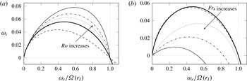
Figure 2 shows the growth rate and frequency of the azimuthal wavenumber
 $m=1$
for a fixed Froude number
 $\mathit{Fr}_{h}=1$
and several positive Rossby numbers from
 $\mathit{Ro}=1$
to
 $\mathit{Ro}=10$
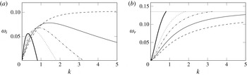
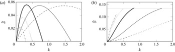
. The growth rate curves for
 $\mathit{Ro}\leqslant 5$
exhibit a bell shape as reported by Gent & McWilliams (Reference Gent and McWilliams1986) and Smyth & McWilliams (Reference Smyth and McWilliams1998). When
 $\mathit{Ro}$
increases from
 $\mathit{Ro}=1$
to
 $\mathit{Ro}=5$
, the most amplified wavenumber increases and the maximum growth rate slightly increases. The unstable wavenumber band also widens when
 $\mathit{Ro}$
increases but, remarkably, it corresponds to a fixed frequency range:
 $0\leqslant {\it\omega}_{r}\leqslant 0.135$
(figure 2
b). Note that the critical value 0.135 is very close to
 $\exp (-2)$
. The reason for this will be seen in § 5.
(a) Growth rate (
 ${\it\omega}_{i}$
) and (b) frequency (
 ${\it\omega}_{r}$
) as function of the vertical wavenumber
 $k$
for the profile (3.1) for
 $m=1$
and
 $\mathit{Fr}_{h}=1$
for different Rossby numbers:
 $\mathit{Ro}=1$
——;
 $\mathit{Ro}=2$
 $\cdots \cdots$
;
 $\mathit{Ro}=3$
– ⋅ – ⋅ –;
 $\mathit{Ro}=5$
——;
 $\mathit{Ro}=10$
- - - -. The horizontal dotted line in (b) shows the cutoff frequency
 ${\it\omega}_{r}=0.135$
.

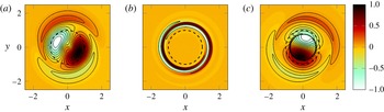
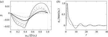
The vertical vorticity of the most unstable perturbation for
 $\mathit{Ro}=1$
is shown in figure 3(a). It exhibits an inner dipolar structure surrounded by outer spiraling perturbations. The inner and outer perturbations have a phase shift and are localized in the regions where the basic vorticity
 ${\it\zeta}$
is negative and positive, respectively. Thus, the perturbations will tend to translate the positive and negative vorticity regions of the basic vortex in different directions. This is a key feature of the mechanism of the GMW instability as discussed by Flierl (Reference Flierl1988) and illustrated in figure 1.
Vertical vorticity of the most unstable eigenmode for the profile (3.1) for
 $m=1$
and (a)
 $\mathit{Fr}_{h}=1,\mathit{Ro}=1,k=0.35$
, (b)
 $\mathit{Fr}_{h}=1,\mathit{Ro}=10,k=100$
and (c)
 $\mathit{Fr}_{h}=2,\mathit{Ro}=1,k=0.1$
. The dashed line represents the radius
 $r=1$
where the sign of the basic vorticity changes. Note that these eigenmodes have been computed for a large but finite Reynolds number
 $\mathit{Re}=10^{6}$
with
 $\mathit{Sc}=1$
in order to resolve the critical layer in (c).

For higher
 $\mathit{Ro}$
, as exemplified in figure 2 by
 $\mathit{Ro}=10$
, the growth rate is no longer maximum for a finite axial wavenumber
 $k$
but increases monotonically with
 $k$
(figure 2
a). The vertical vorticity of the eigenmode for large
 $k$
is then strongly localized at a particular radius (figure 3
b). As shown by Smyth & McWilliams (Reference Smyth and McWilliams1998), this corresponds to the centrifugal instability which is most unstable for
 $k\rightarrow \infty$
. Indeed, the minimum of the Rayleigh discriminant
 ${\it\phi}=(2{\it\Omega}+2/\mathit{Ro})({\it\zeta}+2/\mathit{Ro})$
is negative when
 $\mathit{Ro}>\exp (2)=7.39$
.
For negative Rossby number, the centrifugal instability is also present when
 $\mathit{Ro}<-1$
since
 $\min ({\it\phi})$
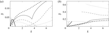
is negative. This can be seen in figure 4 where the growth rate and frequency are displayed for several negative Rossby numbers at
 $\mathit{Fr}_{h}=1$
. The growth rate increases monotonically with
 $k$
for large
 $k$
when
 $\mathit{Ro}<-1$
, whereas for
 $\mathit{Ro}\geqslant -1$
, the growth rate is maximum for a finite wavenumber
 $k$
. Interestingly, there are two distinct and independent branches for
 $\mathit{Ro}=-3$
and
 $\mathit{Ro}=-5$
(figure 4): the GMW instability branch at low
 $k$
and the centrifugal instability branch at large
 $k$
. As seen in figure 4(b), the frequencies of these two branches differ significantly. In contrast, for
 $\mathit{Ro}=-10$
and
 $\mathit{Ro}=-15$
, the two branches are merged into a single continuous one with similar frequencies. Remarkably, the maximum frequency of the GMW instability branch is still
 ${\it\omega}_{r}=0.135$
independently of
 $\mathit{Ro}$
for
 $\mathit{Ro}\geqslant -5$
(figure 4
b).
(a) Growth rate (
 ${\it\omega}_{i}$
) and (b) frequency (
 ${\it\omega}_{r}$
) as function of the vertical wavenumber for the profile (3.1) for
 $m=1$
and
 $\mathit{Fr}_{h}=1$
for different Rossby numbers:
 $\mathit{Ro}=-0.5$
- - - -;
 $\mathit{Ro}=-1$
——;
 $\mathit{Ro}=-3$
 $\cdots \cdots$
;
 $\mathit{Ro}=-5$
– ⋅ – ⋅ –;
 $\mathit{Ro}=-10$
——;
 $\mathit{Ro}=-15$
- - - -. The horizontal dotted line in (b) shows the cutoff frequency
 ${\it\omega}_{r}=0.135$
.

The effect of the Froude number for a fixed Rossby number
 $\mathit{Ro}=1$
is now displayed in figure 5. The maximum growth rate is almost independent of the Froude number when
 $\mathit{Fr}_{h}\leqslant 1$
(figure 5
a). The unstable frequency range also remains the same
 $0\leqslant {\it\omega}_{r}\leqslant 0.135$
even if the upper vertical wavenumber cutoff varies (figure 5
b). However, when
 $\mathit{Fr}_{h}$
is increased above unity, the maximum growth rate decreases abruptly and the unstable frequency range shrinks. As illustrated in figure 3(c), the vertical vorticity of the most unstable perturbation for
 $\mathit{Fr}_{h}=2$
still exhibits a dipolar structure as for
 $\mathit{Fr}_{h}\leqslant 1$
, but there is an additional circular region of rapid variation at a particular radius. This corresponds to a singularity of (2.2) which occurs at the radius where
 $s(r_{c2})=1/\mathit{Fr}_{h}$
, i.e.
 $r_{c2}=0.8$
for
 $\mathit{Fr}_{h}=2$
. Since such a critical layer singularity is regularized in the presence of viscous and diffusive effects, the eigenmode in figure 3(c) has been computed from the linearized Navier–Stokes equations by a Chebyshev pseudo-spectral method for
 $\mathit{Re}=10^{6}$
and
 $\mathit{Sc}={\it\nu}/D=1$
. In the next section, we will show that the growth rate is strongly reduced when
 $\mathit{Fr}_{h}>1$
because of the damping due to this critical layer.
(a) Growth rate (
 ${\it\omega}_{i}$
) and (b) frequency (
 ${\it\omega}_{r}$
) as function of the vertical wavenumber
 $k$
for the profile (3.1) for
 $m=1$
and
 $\mathit{Ro}=1$
for different Froude numbers:
 $\mathit{Fr}_{h}=0.25$
- - - -;
 $\mathit{Fr}_{h}=0.5$
——;
 $\mathit{Fr}_{h}=1$
——;
 $\mathit{Fr}_{h}=1.5$
 $\cdots \cdots$
;
 $\mathit{Fr}_{h}=2$
– ⋅ – ⋅ –. The horizontal dotted line in (b) shows the cutoff frequency
 ${\it\omega}_{r}=0.135$
.

The separate effects of the Rossby number for
 $\mathit{Fr}_{h}=1$
and the Froude number for
 $\mathit{Ro}=1$
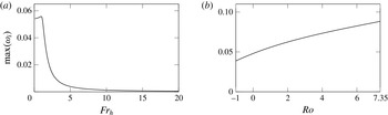
on the maximum growth rate are summarized in figure 6. In figure 6(a), we see that the maximum growth rate continues to decrease when the Froude number is large but it remains positive even for the largest Froude number investigated:
 $\mathit{Fr}_{h}=20$
. The maximum growth rate increases monotonically with
 $\mathit{Ro}$
(figure 6
b): it is approximately doubled from
 $\mathit{Ro}=-1$
to
 $\mathit{Ro}=7.39$
. Only the Rossby number range:
 $-1<Ro<7.39$
is shown in figure 6(b) since outside this range, the vortex is centrifugally unstable. The centrifugal instability is then dominant over the GMW instability (figures 2
a, 4
a) except close to the thresholds
 $\mathit{Ro}=-1$
and
 $\mathit{Ro}=7.39$
.
Maximum growth rate for the profile (3.1) for
 $m=1$
as a function of (a)
 $\mathit{Fr}_{h}$
for
 $\mathit{Ro}=1$
, and (b)
 $\mathit{Ro}$
for
 $\mathit{Fr}_{h}=1$
.

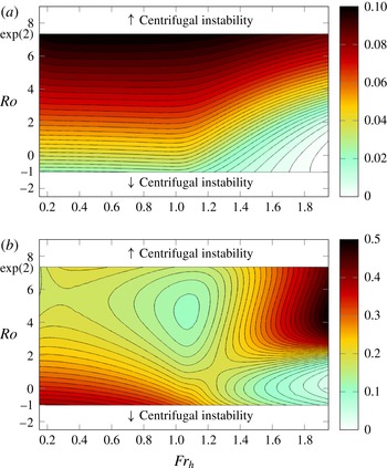
(a) Maximum growth rate and (b) scaled most amplified axial wavenumber
 $k\mathit{Fr}_{h}/|\mathit{Ro}|$
as a function of
 $\mathit{Fr}_{h}$
and
 $\mathit{Ro}$
for the profile (3.1) and for
 $m=1$
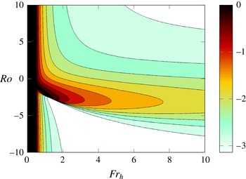
. The contour interval is 0.002 in (a) and 0.007 in (b).

Finally, the combined effects of
 $\mathit{Ro}$
and
 $\mathit{Fr}_{h}$
on the maximum growth rate and the most amplified wavenumber
 $k$
of the GMW instability are depicted in figure 7. The effect of the Froude number is the same independently of
 $\mathit{Ro}$
: the maximum growth rate is independent of
 $\mathit{Fr}_{h}$
for
 $\mathit{Fr}_{h}\leqslant 1$
and decreases abruptly with
 $\mathit{Fr}_{h}$
when
 $\mathit{Fr}_{h}>1$
. The monotonic increase of
 $\max ({\it\omega}_{i})$
with
 $\mathit{Ro}$
is also observed whatever
 $\mathit{Fr}_{h}$
. The most amplified wavenumber has been scaled by
 $\mathit{Fr}_{h}/|\mathit{Ro}|$
in figure 7(b). With this scaling, we see that it varies little and is around
 $k\mathit{Fr}_{h}/|\mathit{Ro}|\approx 0.25{-}0.45$
regardless of
 $\mathit{Fr}_{h}$
and
 $\mathit{Ro}$
.
4. Long-wavelength asymptotic analyses
As seen in § 3, the GMW instability for the Carton and McWilliams profile (3.1) starts at
 $k=0$
, i.e. it is of a long-wavelength nature. For
 $k=0$
, an exact solution of (2.2) for
 $m=1$
which derives from the translational invariance is
 ${\it\varphi}=r({\it\Omega}-{\it\omega})$
(Michalke & Timme Reference Michalke and Timme1967). Using this solution at leading order, the frequency and eigensolution of the azimuthal wavenumber
 $m=1$
can be computed for small wavenumber
 $k$
by means of an asymptotic expansion. A similar asymptotic analysis has been performed in stratified rotating fluids for vortices with non-zero circulation (Billant Reference Billant2010). Using the present non-dimensionalisation and definition of
 $\mathit{Fr}_{h}$
and
 $\mathit{Ro}$
(see § 2), the frequency has been found to be
 $$\begin{eqnarray}{\it\omega}=2a\left(\frac{k{\it\beta}_{0}}{2}\right)^{2}\left[-\!\ln \left(\frac{k|{\it\beta}_{0}|}{2}\right)+\frac{{\it\delta}(\mathit{Fr}_{h},\mathit{Ro})}{a^{2}}-{\it\gamma}_{e}\right],\end{eqnarray}$$
up to order
 $k^{2}$
, where
 $a=\hat{{\it\Gamma}}/(2{\rm\pi}R^{2}{\it\Omega}_{0})$
with
 $\hat{{\it\Gamma}}$
the dimensional circulation,
 ${\it\beta}_{0}=2\mathit{Fr}_{h}/\mathit{Ro}$
and
 ${\it\gamma}_{e}=0.5772$
is the Euler constant. The constant
 ${\it\delta}$
is given by
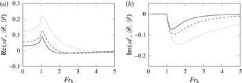
 $$\begin{eqnarray}{\it\delta}(\mathit{Fr}_{h},\mathit{Ro})=\frac{\mathscr{A}(\mathit{Fr}_{h})\mathit{Ro}^{2}}{4}+\mathscr{B}(\mathit{Fr}_{h})\mathit{Ro}+\mathscr{D}(\mathit{Fr}_{h}),\end{eqnarray}$$
with
 $$\begin{eqnarray}\displaystyle & \displaystyle \mathscr{A}(\mathit{Fr}_{h})=\int _{0}^{\infty }\frac{{\it\xi}^{3}{\it\Omega}^{4}}{1-\mathit{Fr}_{h}^{2}{\it\Omega}^{2}}\,\text{d}{\it\xi}, & \displaystyle\end{eqnarray}$$
 $$\begin{eqnarray}\displaystyle & \displaystyle \mathscr{B}(\mathit{Fr}_{h})=\int _{0}^{\infty }\frac{{\it\xi}^{3}{\it\Omega}^{3}}{1-\mathit{Fr}_{h}^{2}{\it\Omega}^{2}}\,\text{d}{\it\xi}, & \displaystyle\end{eqnarray}$$
 $$\begin{eqnarray}\displaystyle & \displaystyle \mathscr{D}(\mathit{Fr}_{h})=\lim _{{\it\eta}_{0}\rightarrow \infty }\int _{0}^{{\it\eta}_{0}}\frac{{\it\xi}^{3}{\it\Omega}^{2}}{1-\mathit{Fr}_{h}^{2}{\it\Omega}^{2}}\,\text{d}{\it\xi}-F_{3}({\it\eta}_{0}), & \displaystyle\end{eqnarray}$$
 $$\begin{eqnarray}F_{3}({\it\eta}_{0})=\int ^{{\it\eta}_{0}}\frac{{\it\xi}^{3}\tilde{{\it\Omega}}^{2}}{1-\mathit{Fr}_{h}^{2}\tilde{{\it\Omega}}^{2}}\,\text{d}{\it\xi},\end{eqnarray}$$
where
 $\tilde{{\it\Omega}}$
denotes the asymptotic form of
 ${\it\Omega}$
for large radius. For vortices with non-zero circulation, we have
 $\tilde{{\it\Omega}}=a/r^{2}$
, giving
 $F_{3}({\it\eta}_{0})\simeq a^{2}\ln {\it\eta}_{0}$
for
 ${\it\eta}_{0}\gg \sqrt{\mathit{Fr }_{h}}$
. The factor
 $a$
appears in (4.1) because time is non-dimensionalised by
 $1/{\it\Omega}_{0}$
instead of
 $2{\rm\pi}R^{2}/\hat{{\it\Gamma}}$
in Billant (Reference Billant2010).
The frequency (4.1) is purely real when
 $\mathit{Fr}_{h}\leqslant 1$
whatever
 $\mathit{Ro}$
. When
 $\mathit{Fr}_{h}>1$
, the integrands in (4.3)–(4.5) are singular at the radius where
 ${\it\Omega}(r_{c2})=1/\mathit{Fr}_{h}$
. This singularity is regularized in the presence of viscous and diffusive effects and can be taken into account in the inviscid limit by bypassing the critical radius in the upper complex plane. The constant
 ${\it\delta}$
is then complex with a negative imaginary part implying that the mode
 $m=1$
is damped. Therefore, the long-wavelength bending mode is at best neutral but never unstable when the circulation is non-zero. However, the formula (4.1) breaks down when
 $a=0$
, i.e. when the angular velocity does not behave as
 ${\it\Omega}\simeq a/r^{2}$
for
 $r\gg 1$
. For this reason, specific asymptotic analyses have been carried out for the Carton and McWilliams profile (3.1) and for a profile of the form
 ${\it\Omega}=a_{n}/r^{2n}$
for
 $r\gg 1$
, where
 $a_{n}$
are
 $n$
constants but
 $n$
is different from unity. For both profiles, two regions need to be considered in order to solve (2.2) asymptotically: an inner region where
 $r\ll 1/k$
and an outer region such that
 $r\gg 1$
. However, the analysis for each profile is different and so they are presented separately.
4.1. Carton and McWilliams vortex
A specificity of the profile (3.1) concerns the location of the critical radius
 $r_{c}$
where
 ${\it\Omega}(r_{c})={\it\omega}$
. When
 ${\it\omega}\ll 1$
and
 ${\it\Omega}\simeq a/r^{2}$
, the critical radius is located at
 $r_{c}\simeq \sqrt{a/{\it\omega}}$
. Hence, since (4.1) shows that
 ${\it\omega}=O(k^{2})$
, we have
 $r_{c}\sim O(1/k)$
, meaning that
 $r_{c}$
is located in the outer region. In contrast, the critical radius for the profile (3.1) is located at
 $r_{c}=\sqrt{-\!\ln {\it\omega}}$
. If we anticipate that
 ${\it\omega}\simeq O(k)$
for the long-wavelength bending mode of the profile (3.1), we can deduce that the critical radius is located in the inner region:
 $r_{c}=O(\sqrt{-\!\ln k})$
.
This asymptotic problem is solved in detail in appendix A and only briefly summarized here. The inner and outer solutions are expanded in the form
 $$\begin{eqnarray}{\it\varphi}={\it\varphi}_{0}+\mathit{Fr}_{h}^{2}k^{2}{\it\varphi}_{2}+\cdots \,,\end{eqnarray}$$
with
 ${\it\varphi}_{0}=r({\it\Omega}-{\it\omega})$
in the inner region. Even if
 ${\it\omega}$
will eventually be small, it is simpler to consider it arbitrary to solve the inner problem. This is the reason why
 ${\it\omega}$
appears in the leading order inner solution
 ${\it\varphi}_{0}$
. The expansion (4.7) is written in power of
 $k\mathit{Fr}_{h}$
for convenience since
 $k$
always appears multiplied by
 $\mathit{Fr}_{h}$
in (2.2). The second order inner solution
 ${\it\varphi}_{2}$
and the outer solution are computed in §§ A.1 and A.2. The behaviour of the inner solution for small
 ${\it\omega}$
and for
 $r\gg 1$
is then determined in § A.3. The matching between the inner and outer solutions for
 $1\ll r\ll 1/k$
and
 ${\it\omega}\ll 1$
is performed in § A.4. This leads to the dispersion relation:
 $$\begin{eqnarray}\displaystyle {\it\omega}^{2} & = & \displaystyle \frac{{\it\delta}k^{2}{\it\beta}_{0}^{2}}{2}\left[-\frac{1}{r_{c}^{2}}+\frac{1}{r_{c}^{4}}(1+\text{i}{\rm\pi}{\it\gamma})+\frac{1}{r_{c}^{6}}\left(\frac{2{\rm\pi}^{2}}{3}-2\text{i}{\rm\pi}{\it\gamma}\right)\right.\nonumber\\ \displaystyle & & \displaystyle \left.-\,\frac{2{\rm\pi}^{2}}{r_{c}^{8}}+O\left(\frac{1}{r_{c}^{10}},k^{2}{\it\beta}_{0}^{2}\ln (k{\it\beta}_{0})\right)\right],\end{eqnarray}$$
where
 ${\it\delta}$
is the constant defined in (4.2) and
 ${\it\gamma}=\text{sgn}({\it\omega}_{i})$
. The terms inside the square brackets in (4.8) correspond to an expansion in inverse power of
 $r_{c}^{2}=-\!\ln {\it\omega}$
. Several orders have been computed since the series converges slowly for
 ${\it\omega}\ll 1$
because of the logarithm. The complex terms
 $\text{i}{\rm\pi}{\it\gamma}/r_{c}^{4}$
and
 $-2\text{i}{\rm\pi}{\it\gamma}/r_{c}^{6}$
come from the presence of the critical radius
 $r_{c}$
.
The dispersion relation (4.8) is implicit since the critical radius depends on
 ${\it\omega}$
. To determine whether or not there exist any solutions, it is first convenient to consider only the first two leading orders in
 $1/r_{c}^{2}$
:
 $$\begin{eqnarray}{\it\omega}^{2}=\frac{{\it\delta}k^{2}{\it\beta}_{0}^{2}}{2}\left[-\frac{1}{r_{c}^{2}}+\frac{1}{r_{c}^{4}}(1+\text{i}{\rm\pi}{\it\gamma})\right].\end{eqnarray}$$
By writing
 ${\it\omega}={\it\rho}\text{e}^{\text{i}{\it\theta}}$
and
 ${\it\delta}={\it\mu}\text{e}^{\text{i}{\it\alpha}}$
, the real and imaginary parts of (4.9) read
 $$\begin{eqnarray}\displaystyle & \displaystyle {\it\rho}^{2}\cos (2{\it\theta}-{\it\alpha})=\frac{{\it\mu}k^{2}{\it\beta}_{0}^{2}}{2}(-{\it\varepsilon}_{{\it\rho}}+{\it\varepsilon}_{{\it\rho}}^{2}), & \displaystyle\end{eqnarray}$$
 $$\begin{eqnarray}\displaystyle & \displaystyle {\it\rho}^{2}\sin (2{\it\theta}-{\it\alpha})=\frac{{\it\mu}k^{2}{\it\beta}_{0}^{2}}{2}{\it\varepsilon}_{{\it\rho}}^{2}({\rm\pi}{\it\gamma}-{\it\theta}), & \displaystyle\end{eqnarray}$$
 ${\it\varepsilon}_{{\it\rho}}=-1/\!\ln {\it\rho}\ll 1$
. Combining (4.10) and (4.11) gives
 $$\begin{eqnarray}\tan (2{\it\theta}-{\it\alpha})=-{\it\varepsilon}_{{\it\rho}}({\rm\pi}{\it\gamma}-{\it\theta})+O({\it\varepsilon}_{{\it\rho}}^{2}).\end{eqnarray}$$
This relation is satisfied if
 $$\begin{eqnarray}{\it\theta}=\frac{{\it\alpha}}{2}+\frac{q{\rm\pi}}{2}-\frac{{\it\varepsilon}_{{\it\rho}}}{4}(2{\rm\pi}{\it\gamma}-{\it\alpha}-q{\rm\pi})+O({\it\varepsilon}_{{\it\rho}}^{2}),\end{eqnarray}$$
where
 $q$
is an integer. Inserting (4.13) into (4.10) then gives an implicit relation for
 ${\it\rho}=|{\it\omega}|$
 $$\begin{eqnarray}{\it\rho}^{2}(-1)^{q}=\frac{{\it\mu}k^{2}{\it\beta}_{0}^{2}}{2}(-{\it\varepsilon}_{{\it\rho}}+{\it\varepsilon}_{{\it\rho}}^{2}+O({\it\varepsilon}_{{\it\rho}}^{3})),\end{eqnarray}$$
which can be satisfied at leading order only if
 $q$
is odd. Hence, the implicit dispersion relation (4.9) can be solved explicitly at leading orders by first choosing a small value for
 ${\it\rho}$
. Then, the corresponding value of
 ${\it\theta}$
and
 $k$
can be obtained directly from (4.13) and (4.14), respectively.
In order to exhibit the behaviour of the solutions, we first focus on the simplest case
 $\mathit{Fr}_{h}\leqslant 1$
for which there is no critical layer
 $r_{c2}$
where
 ${\it\Omega}(r_{c2})=1/\mathit{Fr}_{h}$
so that
 ${\it\delta}$
is purely real and positive, i.e.
 ${\it\alpha}=0$
. Then, (4.13) yields two solutions:
 ${\it\theta}={\rm\pi}/2-{\it\varepsilon}_{{\it\rho}}{\rm\pi}/4$
for
 $q=1$
and
 ${\it\theta}=-{\rm\pi}/2+{\it\varepsilon}_{{\it\rho}}{\rm\pi}/4$
for
 $q=-1$
. Other values of
 $q$
are not relevant since
 $-{\rm\pi}\leqslant {\it\theta}\leqslant {\rm\pi}$
. The dispersion relation (4.9) has therefore two solutions which are complex conjugates of each other, one unstable and the other stable, which can be written in the form:
 $$\begin{eqnarray}\displaystyle & \displaystyle {\it\omega}={\it\rho}\text{e}^{\text{i}{\it\theta}}={\it\rho}\left[\frac{{\it\varepsilon}_{{\it\rho}}}{4}{\rm\pi}+\text{i}\right], & \displaystyle\end{eqnarray}$$
 $$\begin{eqnarray}\displaystyle & \displaystyle {\it\omega}={\it\rho}\left[\frac{{\it\varepsilon}_{{\it\rho}}}{4}{\rm\pi}-\text{i}\right], & \displaystyle\end{eqnarray}$$
 ${\it\rho}$
(and
 ${\it\varepsilon}_{{\it\rho}}=-1/\!\ln {\it\rho}$
) is related to
 $k$
through (4.14). The frequency
 ${\it\omega}_{r}$
is positive and
 $O({\it\varepsilon}_{{\it\rho}})$
smaller than the growth rate.
We now consider the case
 $\mathit{Fr}_{h}>1$
for which
 ${\it\delta}$
is complex with a negative imaginary part, i.e.
 $-{\rm\pi}<{\it\alpha}\leqslant 0$
because of the critical layer
 $r_{c2}$
where
 ${\it\Omega}(r_{c2})=1/\mathit{Fr}_{h}$
. In this case, the two solutions (4.15) and (4.16) become at leading order:
 $$\begin{eqnarray}\displaystyle & \displaystyle {\it\omega}={\it\rho}\left[-\!\sin \frac{{\it\alpha}}{2}+\frac{{\it\varepsilon}_{{\it\rho}}}{4}({\rm\pi}-{\it\alpha})\cos \frac{{\it\alpha}}{2}+\text{i}\left(\cos \frac{{\it\alpha}}{2}+\frac{{\it\varepsilon}_{{\it\rho}}}{4}({\rm\pi}-{\it\alpha})\sin \frac{{\it\alpha}}{2}\right)\right], & \displaystyle\end{eqnarray}$$
 $$\begin{eqnarray}\displaystyle & \displaystyle {\it\omega}={\it\rho}\left[\sin \frac{{\it\alpha}}{2}+\frac{{\it\varepsilon}_{{\it\rho}}}{4}({\rm\pi}+{\it\alpha})\cos \frac{{\it\alpha}}{2}-\text{i}\left(\cos \frac{{\it\alpha}}{2}+\frac{{\it\varepsilon}_{{\it\rho}}}{4}({\rm\pi}+{\it\alpha})\sin \frac{{\it\alpha}}{2}\right)\right], & \displaystyle\end{eqnarray}$$
 ${\it\rho}$
can be still determined as a function of
 $k$
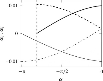
by means of (4.14). The two solutions are no longer complex conjugates of each other. If we consider a fixed value of
 ${\it\rho}$
, the relation (4.17), which is illustrated in figure 8, shows that the growth rate of the unstable solution decreases when
 ${\it\alpha}$
decreases from zero, meaning that the instability is damped by the critical layer at
 $r_{c2}$
. From (4.13), we can deduce that the growth rate goes to zero (i.e.
 ${\it\theta}=0$
) when
 ${\it\alpha}\simeq -{\rm\pi}+{\rm\pi}{\it\varepsilon}_{{\it\rho}}$
(dotted line in figure 8). When
 ${\it\alpha}$
decreases further below this critical value, (4.13) no longer has a solution for
 $q=1$
, i.e. the solution (4.17) does not exist anymore because the integration path has been assumed to be on the real axis. However, the solution (4.17) could be continued by deforming the integration path in the upper complex plane above the critical radius
 $r_{c}$
. The mode (4.17) would be then non-regular and damped since the critical radius would be located between the integration path and the real axis. In contrast, the stable solution (4.18) (thin lines in figure 8) exists in the whole range
 $-{\rm\pi}<{\it\alpha}<0$
. The damping rate of this mode is reduced when
 ${\it\alpha}$
decreases and vanishes for
 ${\it\alpha}=-{\rm\pi}$
. Its frequency becomes negative as soon as
 ${\it\alpha}<-{\it\varepsilon}_{{\it\rho}}{\rm\pi}/2$
.
Frequency
 ${\it\omega}_{r}$
(dashed lines) and growth rate
 ${\it\omega}_{i}$
(solid lines) predicted by (4.17) (thick lines) and (4.18) (thin lines) as a function of
 ${\it\alpha}=\arg ({\it\delta})$
for a given value of
 ${\it\rho}=0.01$
. The dotted line shows the critical value for which the solution (4.17) disappears.

Figure 9 shows
 ${\it\alpha}$
as a function of
 $\mathit{Fr}_{h}$
and
 $\mathit{Ro}$
. We see that
 ${\it\alpha}$
decreases and tends to
 ${\it\alpha}=-{\rm\pi}$
for large Froude number for any Rossby number. This decay occurs slower when
 $\mathit{Ro}$
is negative and moderate, i.e.
 $-5\leqslant \mathit{Ro}\leqslant 0$
. Hence, for a given value of
 ${\it\varepsilon}_{{\it\rho}}=-1/\!\ln |{\it\omega}|$
, the growth rate of the unstable mode (4.17) should vanish for large Froude number when
 ${\it\alpha}\simeq -{\rm\pi}+{\rm\pi}{\it\varepsilon}_{{\it\rho}}$
. This critical Froude number increases and tends to infinity since
 ${\it\alpha}\rightarrow -{\rm\pi}$
as
 $|{\it\omega}|$
decreases to zero. In other words, the instability should be totally suppressed only as the Froude number tends to infinity.
Contours of
 ${\it\alpha}=\arg ({\it\delta})$
as a function of
 $\mathit{Fr}_{h}$
and
 $\mathit{Ro}$
for the profile (3.1). The contour interval is 0.3.

However, it should be noted that the dispersion relation (4.8) (and (4.9)) is no longer valid when
 $\mathit{Fr}_{h}=\infty$
when
 $\mathit{Ro}$
is finite. The behaviour of the inner solution for large radius is indeed different in this case so that the matching performed to derive (4.8) breaks down. Nevertheless, it remains valid when
 $\mathit{Ro}=\infty$
i.e. for a stratified non-rotating fluid and this is considered in appendix B. The evolution of the two solutions of (4.8) is studied as a function of
 $\mathit{Fr}_{h}$
. In particular, it is shown that in the limit
 $\mathit{Fr}_{h}=\infty$
, there remains only one solution with a negative and purely real frequency
 ${\it\omega}$
as predicted by (4.17) and (4.18).
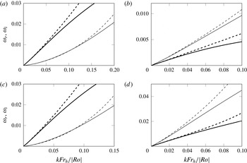
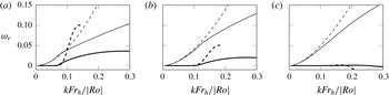
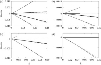
We now compare the prediction of the full long-wavelength dispersion relation (4.8) for the unstable mode to the numerical results. Figure 10(a) shows the asymptotic and numerical growth rates and frequencies for small Froude and Rossby numbers (
 $\mathit{Fr}_{h}=0.1,\mathit{Ro}=0.1$
) approaching the quasi-geostrophic limit. We see that they agree but only in a limited range of small wavenumbers:
 $k\mathit{Fr}_{h}/\mathit{Ro}\lesssim 0.05$
. This relatively rapid divergence is due to the fact that the asymptotic dispersion relation (4.8) has been partly obtained as an expansion in power of the parameter
 $1/r_{c}^{2}=-1/\!\ln {\it\omega}$
. Because of the logarithm, this parameter can actually be not very small even if
 ${\it\omega}$
is small so that the convergence of the asymptotics is slow. Other comparisons for finite Froude and Rossby numbers are displayed in figure 10(b–d). The slopes of the frequency and growth rate at
 $k=0$
predicted by the asymptotics agree with the numerical results for all the values of
 $\mathit{Fr}_{h}$
and
 $\mathit{Ro}$
investigated. As predicted by (4.17), the growth rate remains positive for sufficiently small
 $k$
even for the largest Froude number investigated
 $\mathit{Fr}_{h}=5$
(figure 10
b). We can see that the slope of the growth rate is smaller than the one of the frequency in figure 10(b,d) in contrast to figure 10(a,c). As shown by (4.17) and figure 8, this occurs for
 ${\it\alpha}\lesssim -{\rm\pi}/2$
, i.e. when
 $\mathit{Fr}_{h}$
is sufficiently larger than unity.
Comparison (thick lines:
 ${\it\omega}_{i}$
; thin lines:
 ${\it\omega}_{r}$
) between numerical results (solid lines) and asymptotic results (dashed lines) for the profile (3.1) for
 $m=1$
for several combinations of
 $\mathit{Fr}_{h}$
and
 $\mathit{Ro}$
: (a)
 $\mathit{Ro}=0.1,\mathit{Fr}_{h}=0.1$
; (b)
 $\mathit{Ro}=-1,\mathit{Fr}_{h}=5$
; (c)
 $\mathit{Ro}=0.2$
,
 $\mathit{Fr}_{h}=1$
; (d)
 $\mathit{Ro}=5,\mathit{Fr}_{h}=2$
.

In summary, we have found that the azimuthal wavenumber
 $m=1$
for the Carton and McWilliams vortex (3.1) is always unstable in the long-wavelength limit for finite
 $\mathit{Ro}$
when
 $\mathit{Fr}_{h}\leqslant 1$
. Thus, even if the GMW instability is dominant only in the centrifugally stable range
 $-1<\mathit{Ro}<7.39$
, it exists for long-wavelengths outside this range of Rossby numbers. When
 $\mathit{Fr}_{h}$
is increased above unity, the GMW instability continues to exist in the long-wavelength limit but is strongly damped by the critical layer where
 ${\it\Omega}(r_{c2})=1/\mathit{Fr}_{h}$
. In the limit
 $\mathit{Ro}=\mathit{Fr}_{h}=\infty$
, the long-wavelength bending mode is neutral with a negative frequency.
4.2. Vortices with algebraic decay of the angular velocity
We now investigate an angular velocity profile which behaves like
 ${\it\Omega}\simeq a_{n}/r^{2n}$
for large radii, where
 $a_{n}$
and
 $n$
are constants. This is the case of the profile
 $$\begin{eqnarray}{\it\Omega}=1/(1+r^{2})^{n},\end{eqnarray}$$
considered by Gent & McWilliams (Reference Gent and McWilliams1986). The interest in this class of profiles lies in the fact that the vertical vorticity derivative
 ${\it\zeta}^{\prime }\simeq 4a_{n}n(n-1)/r^{2n+1}$
for large radius can be positive or negative depending on whether
 $n>1$
or
 $n<1$
, respectively. This will allow us to highlight the role of the sign of
 ${\it\zeta}^{\prime }$
at the critical radius
 $r_{c}$
. However, this asymptotic analysis can be carried out analytically only when
 $n=1+{\it\varepsilon}$
with
 $|{\it\varepsilon}|\ll 1$
, i.e. when
 ${\it\zeta}^{\prime }(r_{c})$
is small. As discussed earlier, Briggs et al. (Reference Briggs, Daugherty and Levy1970), Schecter et al. (Reference Schecter, Montgomery and Reasor2002) and Schecter & Montgomery (Reference Schecter and Montgomery2003) also used this assumption to derive their expressions for the growth/decay rate due to the critical layer. In contrast to § 4.1, the critical radius
 $r_{c}$
is located in the outer region for small wavenumber since
 $r_{c}\simeq (a_{n}/{\it\omega})^{1/2n}\simeq O(1/k^{1/n})$
, where it has been anticipated that
 ${\it\omega}\simeq O(k^{2})$
at leading order. This asymptotic analysis is carried out in detail in appendix C. It gives the frequency up to orders
 $k^{2}$
and
 ${\it\varepsilon}$
in the form:
 $$\begin{eqnarray}{\it\omega}={\it\omega}^{(0)}+{\it\varepsilon}{\it\omega}^{(1)}+O({\it\varepsilon}^{2}),\end{eqnarray}$$
where
 $$\begin{eqnarray}\displaystyle & \displaystyle {\it\omega}^{(0)}=2a_{n}\left(\frac{k{\it\beta}_{0}}{2}\right)^{2}\left(-\!\ln \left(\frac{k|{\it\beta}_{0}|}{2}\right)+\frac{{\it\delta}}{a_{n}^{2}}-{\it\gamma}_{e}\right), & \displaystyle\end{eqnarray}$$
 $$\begin{eqnarray}\displaystyle & \displaystyle {\it\omega}^{(1)}=2a_{n}\left(\frac{k{\it\beta}_{0}}{2}\right)^{2}\left[1-E-{\it\gamma}_{e}-\frac{{\it\delta}}{a_{n}^{2}}+\ln 2+\ln (k|{\it\beta}_{0}|)\left(1-2{\it\gamma}_{e}-\frac{2{\it\delta}}{a_{n}^{2}}+2\ln 2\right)\right], & \displaystyle \nonumber\\ \displaystyle & & \displaystyle\end{eqnarray}$$
 $E$
is a constant defined by
 $$\begin{eqnarray}\displaystyle E & = & \displaystyle \lim _{{\it\eta}_{0}\rightarrow 0}\int _{\infty }^{{\it\eta}_{0}/k}\frac{4\text{K}_{1}^{2}({\it\beta}_{0}kr)}{r(1-{\it\omega}^{(0)}r^{2}/a_{n})}\,\text{d}r+\frac{2}{{\it\beta}_{0}^{2}{\it\eta}_{0}^{2}}\nonumber\\ \displaystyle & & \displaystyle -\,2\ln ({\it\eta}_{0}{\it\beta}_{0})\left[-1+2{\it\gamma}_{e}+\frac{2{\it\omega}^{(0)}}{k^{2}{\it\beta}_{0}^{2}a_{n}}+\ln \left(\frac{{\it\eta}_{0}{\it\beta}_{0}}{4}\right)\right].\end{eqnarray}$$
The leading term
 ${\it\omega}^{(0)}$
in (4.20) corresponds to (4.1). When
 ${\it\varepsilon}$
is non-zero and
 $\mathit{Fr}_{h}\leqslant 1$
, all the terms in (4.20) are real except the constant
 $E$
. As seen in (4.23), this constant can indeed be complex since the integrand is singular at the critical radius where
 ${\it\Omega}(r_{c})-{\it\omega}^{(0)}\equiv a_{n}/r_{c}^{2}-{\it\omega}^{(0)}=0$
. Assuming that the integration path in (4.23) is deformed in the upper complex plane since
 ${\it\Omega}^{\prime }(r_{c})<0$
, the imaginary part of
 $E$
is then
 $$\begin{eqnarray}E_{i}=\text{Im}(E)={\rm\pi}a_{-1},\end{eqnarray}$$
with
 $a_{-1}$
the residue at
 $r_{c}$
,
 $$\begin{eqnarray}a_{-1}=-2\text{K}_{1}^{2}(k{\it\beta}_{0}r_{c}).\end{eqnarray}$$
Hence, we see that
 $E_{i}$
is negative, implying that the growth rate
 ${\it\omega}_{i}=-{\it\varepsilon}a_{n}k^{2}{\it\beta}_{0}^{2}E_{i}/2$
is positive or negative when
 ${\it\varepsilon}>0$
or
 ${\it\varepsilon}<0$
, respectively. Note that there also exists a decaying mode when
 ${\it\varepsilon}>0$
which is the complex conjugate of the unstable mode. This can be obtained by integration in the lower complex plane. This stable mode is regular since the integration path can be deformed continuously from the real axis without encountering the critical radius
 $r_{c}$
, unlike the stable mode when
 ${\it\varepsilon}<0$
.
When
 $\mathit{Fr}_{h}>1$
, the additional critical radius
 ${\it\Omega}(r_{c2})=1/\mathit{Fr}_{h}$
is present as for the Carton and McWilliams vortex (§ 4.1). Its effect appears again in (4.20) through
 ${\it\delta}_{i}$
the imaginary part of the constant
 ${\it\delta}$
. The destabilizing effect of the critical radius
 ${\it\Omega}(r_{c})={\it\omega}^{(0)}$
when
 ${\it\varepsilon}>0$
is then in competition with the stabilizing effect due to
 $r_{c2}$
. Assuming that
 ${\it\delta}_{i}$
is small, the growth rate is then at leading order
 $$\begin{eqnarray}{\it\omega}_{i}=\frac{a_{n}k^{2}{\it\beta}_{0}^{2}}{2}\left(\frac{{\it\delta}_{i}}{a_{n}^{2}}-{\it\varepsilon}E_{i}\right).\end{eqnarray}$$
Therefore, there will be an instability in the long-wavelength limit only when
 $$\begin{eqnarray}\frac{{\it\delta}_{i}}{a_{n}^{2}}-{\it\varepsilon}{\rm\pi}a_{-1}>0.\end{eqnarray}$$
From (4.3)–(4.5), we can obtain
 $$\begin{eqnarray}{\it\delta}_{i}=\frac{{\rm\pi}r_{c2}^{3}}{2{\it\Omega}^{\prime }(r_{c2})}\left[\frac{\mathit{Ro}}{2\mathit{Fr}_{h}}+1\right]^{2}\frac{1}{\mathit{Fr}_{h}^{3}}.\end{eqnarray}$$
This shows that
 ${\it\delta}_{i}$
depends only on (
 $\mathit{Fr}_{h},\mathit{Ro}$
) for a given velocity profile. In contrast, the residue
 $a_{-1}$
depends also on
 $kr_{c}$
and therefore varies with (
 ${\it\omega}^{(0)},k$
). Thus, the condition (4.27) depends on the four parameters (
 $\mathit{Fr}_{h},\mathit{Ro},{\it\omega}^{(0)},k$
). However, if we consider a very small wavenumber
 $k$
, we have from (4.21):
 ${\it\omega}^{(0)}\simeq -a_{n}{\it\beta}_{0}^{2}k^{2}\ln ({\it\beta}_{0}k/2)/2$
at leading order for finite Rossby and Froude number. This implies that
 $k{\it\beta}_{0}r_{c}=k{\it\beta}_{0}a_{n}/\sqrt{{\it\omega}^{(0)}}\simeq [-\!\ln ({\it\beta}_{0}k/2)/2]^{-1/2}$
showing that
 $k{\it\beta}_{0}r_{c}$
tends to zero as
 $k$
tends to zero. Hence, we can estimate the residue as
 $$\begin{eqnarray}a_{-1}=-2\text{K}_{1}^{2}(k{\it\beta}_{0}r_{c})\simeq \ln \left(\frac{{\it\beta}_{0}k}{2}\right).\end{eqnarray}$$
This shows that
 $|a_{-1}|$
tends to infinity when
 $k$
vanishes. In contrast, (4.28) is independent of the wavenumber. Therefore, if
 ${\it\varepsilon}>0$
, we can deduce that for any finite Rossby and Froude numbers, the condition (4.27) will be satisfied for sufficiently small wavenumber. In other words, there should always exist an instability in the long-wavelength limit for finite Froude and Rossby numbers as for the Carton and McWilliams vortex (§ 4.1). However, when either
 $\mathit{Ro}=\infty$
or
 $\mathit{Fr}_{h}=\infty$
, the previous condition does not apply and it would be necessary to carry out specific analyses for these limits. In the particular limit
 $\mathit{Ro}=\mathit{Fr}_{h}=\infty$
, it is known that the long-wavelength bending mode when
 $n=1$
is neutral with a negative frequency (Widnall et al.
Reference Widnall, Bliss, Zalay, Olsen, Goldburg and Rogers1971; Saffman Reference Saffman1992) as for the Carton and McWilliams vortex (appendix B). Hence, no critical radius exists.
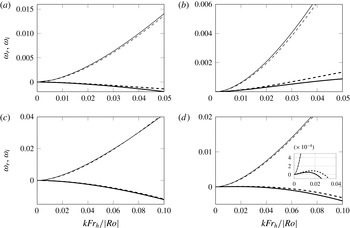
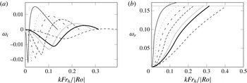
Figure 11 shows some comparisons between the predictions of (4.20) and numerical results for the angular velocity profile (4.19) for
 $n=0.9$
(a,c) and
 $n=1.1$
(b,d) for two Froude numbers
 $\mathit{Fr}_{h}=0.5$
(a,b) and
 $\mathit{Fr}_{h}=1.3$
(c,d) for a fixed Rossby number
 $\mathit{Ro}=1$
. In each case, a good agreement is found for small wavenumber. When
 $\mathit{Fr}_{h}=0.5$
, there is an instability in the long-wavelength limit when
 $n=1.1$
(figure 11
b) while the case
 $n=0.9$
(figure 11
a) is stable since
 ${\it\varepsilon}$
is positive and negative, respectively. When
 $\mathit{Fr}_{h}=1.3$
, the value
 $n=0.9$
(figure 11
c) is still stable. The value
 $n=1.1$
for
 $\mathit{Fr}_{h}=1.3$
(figure 11
d) seems also stable but if we examine the small wavenumber region more closely, we see that the growth rate is actually positive, as predicted by (4.27). The maximum growth rate is however very small. When
 $\mathit{Fr}_{h}$
is increased further, the maximum growth rate continues to decrease but, strictly speaking, it should remain positive for sufficiently small
 $k$
when
 $\mathit{Fr}_{h}$
is finite.
Frequency
 ${\it\omega}_{r}$
(thin lines) and growth rate
 ${\it\omega}_{i}$
(thick lines) for
 $m=1$
for the profile (4.19), for
 $n=0.9$
(a,c) and
 $n=1.1$
(b,d) for
 $\mathit{Fr}_{h}=0.5$
(a,b) and
 $\mathit{Fr}_{h}=1.3$
(c,d) for
 $\mathit{Ro}=1$
. The solid and dashed lines show the numerical and asymptotic results, respectively. The insert in (d) displays a close-up view for small
 $k\mathit{Fr}_{h}/|\mathit{Ro}|$
.

5. General instability condition
The long-wavelength asymptotic analysis performed in § 4.2 can be generalized to angular velocity profiles differing from the form
 ${\it\Omega}=a_{n}/r^{2(1+{\it\varepsilon})}$
for large radius but still with a weak gradient of vorticity
 ${\it\zeta}^{\prime }$
for large radius i.e.
 ${\it\Omega}=a_{n}/r^{2}+{\it\varepsilon}{\it\Omega}_{1}(r)$
so that
 ${\it\zeta}=O({\it\varepsilon})$
. As shown in § C.6, the growth rate
 ${\it\omega}_{i}$
is then at leading order
 $$\begin{eqnarray}{\it\omega}_{i}=\frac{a_{n}k^{2}{\it\beta}_{0}^{2}}{2}\left[\frac{{\it\delta}_{i}}{a_{n}^{2}}-\frac{{\rm\pi}{\it\zeta}^{\prime }(r_{c})\text{K}_{1}^{2}(k{\it\beta}_{0}r_{c})}{{\it\Omega}^{\prime }(r_{c})}\right].\end{eqnarray}$$
Since
 ${\it\delta}_{i}\leqslant 0$
, a general necessary condition for instability of the bending mode in the long-wavelength limit is that there exists a critical radius
 $r_{c}$
where
 ${\it\Omega}(r_{c})={\it\omega}$
with
 ${\it\zeta}^{\prime }(r_{c})>0$
since
 ${\it\Omega}^{\prime }(r_{c})\simeq -2a_{n}/r_{c}^{3}<0$
. This instability condition is sufficient when
 $\mathit{Fr}_{h}\leqslant 1$
since
 ${\it\delta}_{i}=0$
. When
 $\mathit{Fr}_{h}>1$
, it can be also sufficient if
 $|{\it\delta}_{i}|/a_{n}^{2}$
is smaller than the destabilizing term (last term of (5.1)) as for the profiles considered in § 4.2. However, this depends on each particular vortex profile and therefore the instability condition will not always be sufficient for
 $\mathit{Fr}_{h}>1$
.
When
 $\mathit{Fr}_{h}<1$
, i.e.
 ${\it\delta}_{i}=0$
, the expression (5.1) closely resembles to the growth rate formula derived for weak vorticity gradient at the critical radius by Schecter et al. (Reference Schecter, Montgomery and Reasor2002) under the quasi-geostrophic approximation and Schecter & Montgomery (Reference Schecter and Montgomery2003) under the asymmetric and hydrostatic balance approximations. However, the formulas of Schecter et al. (Reference Schecter, Montgomery and Reasor2002) and Schecter & Montgomery (Reference Schecter and Montgomery2003) are implicit since they require prior numerical computation of the eigenfunction and frequency for zero outer vorticity gradient. These formula can become explicit only for the Rankine vortex profile with skirt (weak outer vorticity field) for which an analytic solution can be found. In this case, these formula in the limit
 $k\ll 1$
become identical to (5.1). In contrast, (5.1) is always explicit for any vortex profiles with small vorticity gradient at large radius. The critical radius is indeed given by
 $r_{c}=\sqrt{a_{n}/{\it\omega}^{(0)}}$
where the frequency at leading order
 ${\it\omega}^{(0)}$
is given explicitly by (4.21). The formula (5.1) is restricted to small wavenumbers
 $k$
, but the formula of Schecter et al. (Reference Schecter, Montgomery and Reasor2002) and Schecter & Montgomery (Reference Schecter and Montgomery2003) are also implicitly restricted to small wavenumbers since the assumption of weak vorticity gradient at the critical radius applies when the critical radius is large, i.e. when the frequency and wavenumber are small for the bending mode. In addition, we emphasize that (5.1) is valid for any finite Froude and Rossby numbers and, therefore, is not restricted to the regime of validity of the asymmetric and hydrostatic balance approximations in contrast to the formula of Schecter & Montgomery (Reference Schecter and Montgomery2003).
It is also worth noting that the instability condition
 ${\it\zeta}^{\prime }(r_{c})>0$
is equivalent to the Rayleigh and Fjortoft necessary criteria for instability in the case of a quasi-geostrophic fluid and a vortex with a monotonically decreasing angular velocity (Gent & McWilliams Reference Gent and McWilliams1986). Indeed, the Rayleigh criterion requires that there exists an inflection point
 $r_{I}$
where
 ${\it\zeta}^{\prime }(r_{I})=0$
while the Fjortoft criterion demands that
 ${\it\zeta}^{\prime }>0$
for
 $r>r_{I}$
and
 ${\it\zeta}^{\prime }<0$
for
 $r<r_{I}$
when
 ${\it\Omega}^{\prime }(r)<0$
for all
 $r$
. Montgomery & Shapiro (Reference Montgomery and Shapiro1995) have extended these criteria to flows under the asymmetric and hydrostatic balance approximations. In contrast, the present asymptotic analysis and resulting instability condition are valid for any finite Froude and Rossby numbers. However, their validity are restricted to small
 $k$
and small vorticity gradient
 ${\it\zeta}^{\prime }(r_{c})$
, in contrast to the Rayleigh and Fjortoft criteria.
In practice, we can show from the numerical results obtained for the profile (3.1) (§ 3) that
 ${\it\zeta}^{\prime }(r_{c})>0$
is a necessary condition for instability of the bending mode for any vertical wavenumber and magnitude of
 ${\it\zeta}^{\prime }(r_{c})$
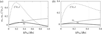
for finite Froude and Rossby numbers. Figure 12(a) shows again the frequency and growth rate for
 $\mathit{Ro}=\mathit{Fr}_{h}=1$
for the profile (3.1) (i.e. corresponding to the bold line in figure 2). The derivative of the vorticity at the critical radius
 ${\it\zeta}^{\prime }(r_{cr})$
is also plotted. Note that only the real part of
 $r_{c}$
is considered since the imaginary part of
 $r_{c}$
is small because
 ${\it\omega}_{i}$
is small. As seen in figure 12(a), the growth rate
 ${\it\omega}_{i}$
and
 ${\it\zeta}^{\prime }(r_{cr})$
are positive in the same range of vertical wavenumbers. Hence, the cutoff wavenumber
 $k_{c}\mathit{Fr}_{h}/|\mathit{Ro}|\simeq 0.8$
corresponds to the limit where
 ${\it\zeta}^{\prime }(r_{c})=0$
, i.e. when the critical radius
 $r_{c}$
becomes equal to the inflection point
 $r_{I}=\sqrt{2}$
. The maximum value of the frequency corresponds therefore to
 ${\it\omega}_{r}={\it\Omega}(r_{I})=0.135$
, as observed in § 3. Figure 13(a), which shows the growth rate as a function of
 ${\it\omega}_{r}/{\it\Omega}(r_{I})$
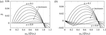
, confirms that the GMW instability occurs if and only if
 $0\leqslant {\it\omega}_{r}/{\it\Omega}(r_{I})\leqslant 1$
for
 $\mathit{Fr}_{h}=1$
for the different Rossby numbers investigated:
 $-0.5\leqslant \mathit{Ro}\leqslant 5$
for which only the GMW instability exists.
Growth rate (——:
 ${\it\omega}_{i}$
) and frequency, (——:
 ${\it\omega}_{r}$
) for the profile (3.1) for
 $m=1$
as a function of
 $k\mathit{Fr}_{h}/|\mathit{Ro}|$
for (a)
 $\mathit{Ro}=\mathit{Fr}_{h}=1$
and (b)
 $\mathit{Ro}=1,\mathit{Fr}_{h}=3$
. The associated vorticity gradient
 ${\it\zeta}^{\prime }(r_{c})$
(- - - -) at the location of the critical radius on the real axis
 $r_{c}$
.

Growth rate as a function of the rescaled frequency
 ${\it\omega}_{r}/{\it\Omega}(r_{I})$
for
 $m=1$
for the profile (3.1) for (a)
 $\mathit{Fr}_{h}=1$
and
 $\mathit{Ro}$
varying:
 $\mathit{Ro}=-0.5$
- - - -;
 $\mathit{Ro}=1$
——;
 $\mathit{Ro}=2$
 $\cdots \cdots$
;
 $\mathit{Ro}=3$
– ⋅ – ⋅ –;
 $\mathit{Ro}=5$
—— and (b)
 $\mathit{Ro}=1$
and
 $\mathit{Fr}_{h}$
varying:
 $\mathit{Fr}_{h}=0.5$
- - - -;
 $\mathit{Fr}_{h}=1$
——;
 $\mathit{Fr}_{h}=1.5$
 $\cdots \cdots$
;
 $\mathit{Fr}_{h}=2$
– ⋅ – ⋅ –;
 $\mathit{Fr}_{h}=3$
——.

Figure 12(b) shows the growth rate and frequency for a Froude number larger than unity:
 $\mathit{Fr}_{h}=3$
. In this case, the unstable wavenumber band corresponds only to a portion of the range where
 ${\it\zeta}^{\prime }(r_{cr})>0$
. This means that the instability condition
 ${\it\zeta}^{\prime }(r_{c})>0$
is necessary but not sufficient. As shown in figure 13(b), the range of rescaled frequency
 ${\it\omega}_{r}/{\it\Omega}(r_{I})$
for which the growth rate is positive is
 $0\leqslant {\it\omega}_{r}/{\it\Omega}(r_{I})\leqslant 1$
only when
 $\mathit{Fr}_{h}\leqslant 1$
. When
 $\mathit{Fr}_{h}>1$
, the upper frequency cutoff is lower than
 ${\it\Omega}(r_{I})$
because of the presence of the other critical radius
 ${\it\Omega}(r_{c2})=1/\mathit{Fr}_{h}$
which is always stabilizing. This frequency cutoff decreases when
 $\mathit{Fr}_{h}$
increases but the asymptotic dispersion relation (4.8) has shown that the instability is never suppressed for sufficiently small frequency
 ${\it\omega}$
for finite
 $\mathit{Fr}_{h}$
and
 $\mathit{Ro}$
for the profile (3.1).
6. Non-isolated vortices
In the previous sections, we have considered vortex profiles that have been shown to be unstable to the GMW instability only when their circulation is zero, i.e. when they are isolated. However, this is not generic and it is possible to have profiles with a non-zero circulation satisfying the GMW instability condition, i.e. a positive vorticity gradient for some radius. The purpose of this section is to investigate numerically the stability of the
 $m=1$
azimuthal wavenumber for these vortices. To this end, we consider a family of vortices with a non-dimensional angular velocity combining a Lamb–Oseen and a Carton–McWilliams profiles:
 $$\begin{eqnarray}{\it\Omega}(r)=a\frac{1-\text{e}^{-r^{2}}}{r^{2}}+(1-a)\text{e}^{-r^{2}},\end{eqnarray}$$
where
 $a$
is proportional to the non-dimensional circulation
 ${\it\Gamma}=2{\rm\pi}a$
. When
 $a=1$
, the vortex is a pure Lamb–Oseen vortex while
 $a=0$
corresponds to a pure Carton–McWilliams vortex. The angular velocity on the vortex axis is independent of
 $a$
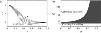
owing to the non-dimensionalisation. The corresponding vorticity
 ${\it\zeta}$
is plotted in figure 14(a) for different values of
 $a$
in the range
 $0\leqslant a\leqslant 1$
. As
 $a$
increases, the negative minimum of vorticity is reduced and disappears for
 $a=1$
. Accordingly, the domain of existence of the centrifugal instability (i.e.
 ${\it\phi}=(2{\it\Omega}+2/\mathit{Ro})({\it\zeta}+2/\mathit{Ro})<0$
) varies with
 $a$
: the upper critical Rossby number increases from
 $\mathit{Ro}_{c}=\exp (2)$
for
 $a=0$
to
 $\mathit{Ro}_{c}=\infty$
for
 $a=1$
(figure 14
b). In contrast, the lower critical Rossby number remains
 $\mathit{Ro}_{c}=-1$
regardless of
 $a$
. As in § 3, we shall study the GMW instability only for the Rossby numbers that are centrifugally stable.
(a) Vorticity profiles corresponding to (6.1) for different values of the parameter
 $a=0:0.2:1$
. (b) Critical Rossby numbers for the centrifugal instability as a function of
 $a$
.

6.1. Effects of the circulation parameter
 $a$
and Froude number
$\mathit{Fr}_{h}$


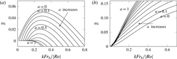
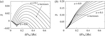
Figure 15 shows the growth rate and frequency of the azimuthal wavenumber
 $m=1$
for
 $\mathit{Fr}_{h}=1,\mathit{Ro}=1$
for various values of the circulation parameter
 $a$
. The most striking feature is that the instability no longer starts at
 $k=0$
when
 $a$
is non-zero. The maximum growth rate and the upper wavelength cutoff also decrease when
 $a$
increases.
(a) Growth rate and (b) frequency as a function of
 $k\mathit{Fr}_{h}/|\mathit{Ro}|$
for the profile (6.1) for
 $m=1$
for
 $\mathit{Fr}_{h}=1$
and
 $\mathit{Ro}=1$
for increasing value of
 $a$
by steps of 0.1.

The stabilization of small wavenumber
 $k$
comes from the fact that the angular velocity now behaves like
 ${\it\Omega}\simeq a/r^{2}$
for large
 $r$
. Indeed, the critical radius
 $r_{c}$
for a given small value of
 ${\it\omega}$
is much larger,
 $r_{c}=\sqrt{a/{\it\omega}}$
, than for
 $a=0$
for which
 $r_{c}=\sqrt{-\!\ln {\it\omega}}$
. This implies that the vorticity gradient at
 $r_{c}$
is
 $O(\text{e}^{-a/{\it\omega}}{\it\omega}^{-3/2})$
, i.e. exponentially small instead of being
 $O({\it\omega}(\ln {\it\omega})^{3/2})$
for
 $a=0$
. Since the growth rate for small wavenumber
 $k$
is directly proportional to
 ${\it\zeta}^{\prime }(r_{c})$
(see (5.1)), it remains exponentially small. The frequency and growth rate are compared to the asymptotic frequency (4.1) and growth rate (5.1) in figure 16 for various values of
 $a$
. The asymptotic frequency (4.1) and the exact frequency agree for small
 $k$
and then differ as soon as the growth rate
 ${\it\omega}_{i}$
begins to rise. Remarkably, the asymptotic growth rate (5.1) also predicts well the lower wavenumber cutoff
 $k_{c}$
at which the exact growth rate rises. However, it then quickly diverges. As seen in figures 16 and 15(a), the lower wavenumber cutoff
 $k_{c}$
increases monotonically with
 $a$
. This behaviour can be understood from the fact that the growth rate becomes non-negligible when
 ${\it\zeta}^{\prime }(r_{c})$
is no longer exponentially small, i.e. approximately when
 $r_{c}\simeq 3$
whatever the value of
 $a$
. Thus, the corresponding frequency
 ${\it\omega}_{c}\simeq a/r_{c}^{2}$
increases linearly with
 $a$
. Since the formula (4.1) turns out to vary weakly when
 $a$
varies (see figure 16), the corresponding wavenumber
 $k_{c}$
, i.e.
 ${\it\omega}(k_{c})=a/r_{c}^{2}$
, increases with
 $a$
.
Comparison (thin lines:
 ${\it\omega}_{r}$
; thick lines:
 ${\it\omega}_{i}$
) between the numerical results (solid lines) and the asymptotic frequency (4.1) (thin dashed lines) and growth rate (5.1) (thick dashed lines) for the profile (6.1) for
 $m=1$
for different values of
 $a$
for
 $\mathit{Ro}=\mathit{Fr}_{h}=1$
: (a)
 $a=0.3$
; (b)
 $a=0.5$
; (c)
 $a=0.8$
.

Figure 17(a) further shows the growth rate as a function of the rescaled frequency
 ${\it\omega}_{r}/{\it\Omega}(r_{I})$
, where
 $r_{I}$
is the inflection point (
 ${\it\zeta}^{\prime }(r_{I})=0$
) determined for each value of
 $a$
. This figure demonstrates that the growth rate vanishes when
 ${\it\omega}_{r}={\it\Omega}(r_{I})$
regardless of
 $a$
. Therefore, the instability occurs only when
 ${\it\zeta}^{\prime }(r_{c})>0$
as already observed for
 $a=0$
in § 5. The growth rate is however negligible for small rescaled frequency
 ${\it\omega}_{r}/{\it\Omega}(r_{I})$
because
 ${\it\zeta}^{\prime }(r_{c})$
is then exponentially small as explained previously.
The rescaled growth rate
 ${\it\omega}_{i}$
as a function of the rescaled frequency
 ${\it\omega}_{r}/{\it\Omega}(r_{I})$
for the profile (6.1) for
 $m=1$
by steps of 0.1 and for
 $\mathit{Ro}=1$
for increasing values of
 $a$
, (a)
 $\mathit{Fr}_{h}=1$
and (b)
 $\mathit{Fr}_{h}=1.2$
.

Figure 18 shows now the growth rate and frequency for a Froude number above unity:
 $\mathit{Fr}_{h}=1.2$
, still for
 $\mathit{Ro}=1$
. The trends when
 $a$
increases are the same as for
 $\mathit{Fr}_{h}=1$
(figure 15). The new feature is that the growth rate is negative for small
 $k$
and then suddenly increases as for
 $\mathit{Fr}_{h}=1$
but the maximum growth rate becomes positive only for
 $a\lesssim 0.7$
. Figure 17(b) shows that the upper wavenumber cutoffs for
 $a\lesssim 0.7$
correspond to the same value of the rescaled frequency
 ${\it\omega}_{r}/{\it\Omega}(r_{I})$
. This critical value is very close to the threshold
 ${\it\omega}_{r}/{\it\Omega}(r_{I})=1$
in contrast to figure 13(b) where the critical rescaled frequencies
 ${\it\omega}_{r}/{\it\Omega}(r_{I})$
were clearly smaller than unity for
 $a=0$
. This difference comes from the fact that the Froude number was larger in figure 13(b),
 $\mathit{Fr}_{h}\geqslant 1.5$
, than in figure 17(b). Another difference is that the growth rate is negative for small wavenumber (i.e. small
 ${\it\omega}_{r}/{\it\Omega}(r_{I})$
) in figure 17(b) while for the Carton and McWilliams profile in figure 13(b), the growth rate remains positive for small
 $k$
even when
 $\mathit{Fr}_{h}>1$
. This stabilization increases with
 $a$
but also with the Froude number. For example, figure 19 displays the growth rate and frequency for a fixed value of the circulation parameter
 $(a=0.7)$
, but different Froude numbers. The maximum growth rate decreases when
 $\mathit{Fr}_{h}$
is above unity and becomes negative for
 $\mathit{Fr}_{h}=1.3$
. Thus, the instability is completely suppressed when the Froude number
 $\mathit{Fr}_{h}$
is above a critical value that depends on the circulation parameter
 $a$
.
(a) Growth rate and (b) frequency as a function of
 $k\mathit{Fr}_{h}/|\mathit{Ro}|$
for the profile (6.1) for
 $m=1$
for
 $\mathit{Fr}_{h}=1.2$
and
 $\mathit{Ro}=1$
for increasing values of
 $a$
by steps of 0.1.

(a) Growth rate and (b) frequency as a function of
 $k\mathit{Fr}_{h}/|\mathit{Ro}|$
for the profile (6.1) for
 $m=1$
for
 $a=0.7,\mathit{Ro}=1$
and varying
 $\mathit{Fr}_{h}$
:
 $\mathit{Fr}_{h}=0.8$
——;
 $\mathit{Fr}_{h}=1$
- - - -;
 $\mathit{Fr}_{h}=1.2$
– ⋅ – ⋅ –;
 $\mathit{Fr}_{h}=1.3$
 $\cdots \cdots$
.

6.2. Effect of the Rossby number
The effect of the Rossby number for a fixed
 $\mathit{Fr}_{h}$
is shown in figure 20. The Rossby number is varied between 0.8 and 50, i.e. within the centrifugally stable range for
 $a=0.7$
(
 $-1<\mathit{Ro}<254$
, see figure 14
b). The maximum growth rate increases with
 $\mathit{Ro}$
as for the Carton and McWilliams vortex (figure 2
a).
Growth rate and frequency as a function of
 $k\mathit{Fr}_{h}/|\mathit{Ro}|$
for the profile (6.1) for
 $m=1$
,
 $a=0.7,\mathit{Fr}_{h}=1.2$
and varying
 $\mathit{Ro}$
:
 $\mathit{Ro}=50$
——;
 $\mathit{Ro}=20$
 $\cdot \cdot \cdot \,\cdot$
;
 $\mathit{Ro}=10$
- - - -;
 $\mathit{Ro}=5$
----;
 $\mathit{Ro}=2$
⋅⋅⋅⋅⋅⋅;
 $\mathit{Ro}=1$
——; and
 $\mathit{Ro}=-0.5$
- - - - (a) growth rate, (b) frequency. The horizontal dotted line in (b) shows the cutoff frequency
 ${\it\omega}_{r}=0.163$
.

Figure 21(a) shows the growth rate as a function of
 ${\it\omega}_{r}/{\it\Omega}(r_{I})$
. All the curves for
 $\mathit{Ro}\leqslant 10$
go to zero very close to the critical value
 ${\it\omega}_{r}/{\it\Omega}(r_{I})=1$
as previously observed. However, the growth rate for
 $\mathit{Ro}=20$
and
 $\mathit{Ro}=50$
remain clearly positive beyond this cutoff. Two examples of eigenmodes for
 $\mathit{Ro}=5$
and
 $\mathit{Ro}=50$
are depicted in figure 21(b). The eigenmode for
 $\mathit{Ro}=50$
exhibits oscillations outside the vortex core in contrast to the one for
 $\mathit{Ro}=5$
. Indeed, when the Rossby number is large, the eigensolution for large radius can be wavelike (see (2.5)) since the parameter
 ${\it\beta}^{2}=(4/\mathit{Ro}^{2}-{\it\omega}^{2})/(1/Fh^{2}-{\it\omega}^{2})$
is negative when
 $|{\it\omega}_{r}|>2/\mathit{Ro}$
(assuming
 ${\it\omega}_{i}=0$
and
 $\mathit{Fr}_{h}<|\mathit{Ro}|/2$
). Such outward radiation of inertia gravity waves lead to the radiative instability as shown by Smyth & McWilliams (Reference Smyth and McWilliams1998), Schecter & Montgomery (Reference Schecter and Montgomery2004), Billant & Le Dizès (Reference Billant and Le Dizès2009), Le Dizès & Billant (Reference Le Dizès and Billant2009), Riedinger et al. (Reference Riedinger, Le Dizès and Meunier2010, Reference Riedinger, Le Dizès and Meunier2011), Park & Billant (Reference Park and Billant2012) and Park & Billant (Reference Park and Billant2013).
(a) Growth rate as a function of the rescaled frequency
 ${\it\omega}_{r}/{\it\Omega}(r_{I})$
for the profile (6.1) for
 $m=1$
,
 $a=0.7$
,
 $\mathit{Fr}_{h}=1.2$
and for different values of
 $\mathit{Ro}$
:
 $\mathit{Ro}=50$
——;
 $\mathit{Ro}=20$
 $\cdot \cdot \cdot \,\cdot$
;
 $\mathit{Ro}=10$
- - - -;
 $\mathit{Ro}=5$
----;
 $\mathit{Ro}=2$
⋅⋅⋅⋅⋅⋅;
 $\mathit{Ro}=1$
——; and
 $\mathit{Ro}=-0.5$
- - - -. (b) Radial velocity of the eigenmode for
 $\mathit{Fr}_{h}=1.2,a=0.7$
for (
 $\mathit{Ro}=50$
,
 $k\mathit{Fr}_{h}/|\mathit{Ro}|=0.086$
: ——) and (
 $\mathit{Ro}=5$
,
 $k\mathit{Fr}_{h}/|\mathit{Ro}|=0.15$
: - - - -).

Since the maximum frequency of the GMW instability is
 $\max ({\it\omega}_{r})={\it\Omega}(r_{I})=0.163$
for
 $a=0.7$
independently of the Rossby and Froude numbers, the critical Rossby number at which the eigenmodes become radiative for some wavenumbers can be estimated at
 $\mathit{Ro}_{c}=2/\max ({\it\omega}_{r})\simeq 12$
. Above this Rossby number, the radiation of inertia gravity waves provides a second source of instability in addition to the critical layer at
 $r_{c}$
. This explains why the mode
 $m=1$
remains unstable beyond the cutoff frequency
 ${\it\omega}_{r}={\it\Omega}(r_{I})$
for
 $\mathit{Ro}=20$
and
 $\mathit{Ro}=50$
in figure 21(a).
7. Conclusion
In this paper, we have investigated the stability of the azimuthal wavenumber
 $m=1$
of an axisymmetric columnar vortex in a stratified and rotating fluid. As shown by Gent & McWilliams (Reference Gent and McWilliams1986) and Smyth & McWilliams (Reference Smyth and McWilliams1998), this azimuthal wavenumber can be unstable to an instability which bends the vortex and leads to the formation of lenticular vortices when the fluid is both stratified and rotating. This three-dimensional instability, called the ‘Gent–McWilliams (GMW) instability’ herein, can occur in the centrifugally stable regime and in the quasi-geostrophic limit. These properties make this instability clearly different from all other known instabilities of columnar axisymmetric vortices: shear instability, centrifugal instability and radiative instability. We have carried out both numerical and asymptotical stability analyses of several vortex profiles to better understand the origin of this instability, to explain why it occurs only in stratified rotating fluids and to derive an instability condition valid outside the quasi-geostrophic regime.
We have first recovered and extended the numerical results of Gent & McWilliams (Reference Gent and McWilliams1986) and Smyth & McWilliams (Reference Smyth and McWilliams1998) for the stability of the azimuthal wavenumber
 $m=1$
for the Carton and McWilliams vortex. In the centrifugally stable regime
 $-1\leqslant \mathit{Ro}\leqslant 7.39$
, we have shown that the maximum growth rate of the GMW instability increases with
 $\mathit{Ro}$
and is independent of
 $\mathit{Fr}_{h}$
for
 $\mathit{Fr}_{h}\leqslant 1$
. In contrast, when
 $\mathit{Fr}_{h}>1$
, the maximum growth rate abruptly decreases with
 $\mathit{Fr}_{h}$
and the eigenmode exhibits a critical layer singularity at the radius where
 ${\it\Omega}(r_{c2})-{\it\omega}=1/\mathit{Fr}_{h}$
. Thereby, the maximum growth rate becomes very small for large Froude number.
These numerical results for the Carton and McWilliams vortex have been completed by an asymptotic analysis of the long-wavelength bending mode. Such mode is a generic mode which derives from the translational invariances in the two-dimensional limit. Hence, its frequency
 ${\it\omega}$
vanishes for
 $k=0$
and can be computed by an asymptotic expansion for small wavenumber
 $k$
. We have found that there exist two long-wavelength bending modes with complex conjugate frequency
 ${\it\omega}$
. The real part of the frequency
 ${\it\omega}_{r}$
and growth rate
 ${\it\omega}_{i}$
of the unstable mode are always positive for finite Rossby and Froude numbers for sufficiently small wavenumbers and are in good agreement with those of the GMW instability computed numerically. This shows that the GMW instability exists for long-wavelengths not only in the centrifugally stable regime:
 $-1\leqslant \mathit{Ro}\leqslant 7.39$
, but also outside of this regime. As the Froude number is increased above unity, the GMW instability continues to exist but the slope of the growth rate with
 $k$
rapidly decreases and becomes negligible because of the damping by the critical layer
 $r_{c2}$
where
 ${\it\Omega}(r_{c2})=1/\mathit{Fr}_{h}$
. The asymptotic results have also allowed us to study the transition from a stratified to an homogeneous fluid in the case of a non-rotating fluid (
 $\mathit{Ro}=\infty$
). We have found that the range of wavenumbers of the unstable long-wavelength bending mode shrinks to zero as the Froude number becomes infinite because of the damping by the critical layer
 $r_{c2}$
. In contrast, the stable long-wavelength bending mode continues to exist as
 $\mathit{Fr}_{h}$
increases. It becomes neutral with a negative frequency as
 $\mathit{Fr}_{h}\rightarrow \infty$
as for the vortices with a non-zero circulation (Widnall et al.
Reference Widnall, Bliss, Zalay, Olsen, Goldburg and Rogers1971).
This asymptotic analysis for the Carton and McWilliams vortex shows that the GMW instability is intimately linked to the existence of a critical radius
 $r_{c}$
where
 ${\it\Omega}(r_{c})={\it\omega}$
as conjectured by Reasor et al. (Reference Reasor, Montgomery and Grasso2004). In order to prove the role played by the sign of the vorticity gradient
 ${\it\zeta}^{\prime }(r_{c})$
at the critical radius
 $r_{c}$
, a second long-wavelength asymptotic analysis has been carried out for vortices exhibiting an algebraic decay of the angular velocity
 ${\it\Omega}\sim a_{n}/r^{2n}$
for large radius, with
 $n$
close to unity. The sign of
 ${\it\zeta}^{\prime }$
is positive if
 $n>1$
and conversely is negative if
 $n<1$
. In the particular case of
 $n=1$
, corresponding to a vortex with a constant circulation, the long-wavelength bending mode for finite Rossby and Froude numbers is known to have a positive frequency
 ${\it\omega}_{r}$
with zero growth rate if
 $\mathit{Fr}_{h}\leqslant 1$
and a negative growth rate if
 $\mathit{Fr}_{h}>1$
because of the critical layer
 $r_{c2}$
where
 ${\it\Omega}(r_{c2})=1/\mathit{Fr}_{h}$
(Billant Reference Billant2010). Here, we have shown that the critical layer
 $r_{c}$
where
 ${\it\Omega}(r_{c})={\it\omega}$
has a positive or negative contribution to the growth rate if
 $n>1$
or
 $n<1$
, respectively. For finite Rossby and Froude numbers, this positive contribution overcomes the negative contribution of the critical layer
 $r_{c2}$
for sufficiently small wavenumber. Thereby, the bending mode is always unstable for sufficiently long wavelength if
 $n>1$
.
For general vorticity profiles, the latter instability condition becomes
 ${\it\zeta}^{\prime }(r_{c})>0$
in agreement with the condition derived by Schecter et al. (Reference Schecter, Montgomery and Reasor2002) and Schecter & Montgomery (Reference Schecter and Montgomery2003) under the quasi-geostrophic and asymmetric balance approximations, respectively. This condition is also equivalent to the Rayleigh inflection point and Fjortoft necessary criteria derived by Gent & McWilliams (Reference Gent and McWilliams1986) in quasi-geostrophic fluids and by Montgomery & Shapiro (Reference Montgomery and Shapiro1995) under the asymmetric balance approximation. However, the necessary instability condition derived herein is not restricted to the quasi-geostrophic or asymmetric balance regimes but is valid for any finite Froude and Rossby numbers. Furthermore, it is necessary and sufficient if
 $\mathit{Fr}_{h}\leqslant 1$
. Nevertheless, we stress that it is restricted to small vorticity gradients
 ${\it\zeta}^{\prime }$
and has been derived in the long-wavelength limit. The numerical results for the Carton & McWilliams (Reference Carton, McWilliams, Nihoul and Jamart1989) vortex show that this necessary instability condition is in practice valid for any axial wavenumber
 $k$
and magnitude of
 ${\it\zeta}^{\prime }$
for finite Froude and Rossby numbers.
Finally, we have investigated the stability of a family of vortices combining a Lamb–Oseen and Carton and McWilliams profiles. These vortices exhibit both positive vorticity gradient
 ${\it\zeta}^{\prime }(r)>0$
for some radii and a non-zero circulation in contrast to the two profiles previously studied. We have shown that these non-isolated vortices are also unstable to the GMW instability in stratified rotating fluids, but only for finite axial wavenumbers as previously observed by Flierl (Reference Flierl1988) for piecewise vorticity profiles in quasi-geostrophic fluids. The long-wavelength limit
 $k\ll 1$
is stable (or marginally unstable) because the vorticity gradient at the critical radius
 ${\it\zeta}^{\prime }(r_{c})$
is exponentially small. This result comes from the fact that the critical radius
 $r_{c}$
is very large when the circulation
 $({\it\Gamma}=2{\rm\pi}a)$
is non-zero and the frequency is small:
 $r_{c}\simeq (a/{\it\omega})^{1/2}$
. Another particularity of the GMW instability for these non-isolated vortices is that the damping effect of the critical radius
 $r_{c2}$
where
 ${\it\Omega}(r_{c2})=1/\mathit{Fr}_{h}$
can completely overcome the destabilizing effect of the critical radius
 $r_{c}$
when the Froude number is sufficiently large.
In summary, the origin of the GMW instability can be traced to a destabilization of the long-wavelength bending mode of a columnar vortex by a critical layer
 $r_{c}$
where
 ${\it\Omega}(r_{c})={\it\omega}/m$
when
 ${\it\zeta}^{\prime }(r_{c})>0$
. This mode is specific to the azimuthal wavenumber
 $m=1$
since it derives from the translational invariances. However, more generally, three-dimensional modes for other azimuthal wavenumbers
 $m\geqslant 2$
could be also destabilized by a critical layer if their frequency range lies in the range
 $0<{\it\omega}/m<{\it\Omega}_{0}$
. Some vortex waves for these azimuthal wavenumbers may indeed have a frequency in this range, both in homogeneous fluids (Kelvin Reference Kelvin1880; Fabre, Sipp & Jacquin Reference Fabre, Sipp and Jacquin2006) and stratified rotating fluids (Schecter et al.
Reference Schecter, Montgomery and Reasor2002; Park & Billant Reference Park and Billant2013). It would be interesting to investigate their stability for vortex profiles satisfying the condition
 ${\it\zeta}^{\prime }(r_{c})>0$
.
Acknowledgements
We thank M. T. Montgomery and W. D. Smyth for their comments to improve this manuscript. This work was supported by the National Research Agency (ANR 2011 Blanc SIMI 5-6 012-02).
Appendix A. Long-wavelength analysis for the Carton and McWilliams vortex in stratified rotating fluids
In this appendix, (2.2) is solved asymptotically for small
 $k\mathit{Fr}_{h}$
and
 $m=1$
for the Carton and McWilliams vortex (3.1) using the expansion (4.7). The frequency
 ${\it\omega}$
is first considered arbitrary for simplicity. Two regions are considered: an inner region where
 $r\ll 1/k$
and an outer region where
 $r\gg 1$
. The matching of the solutions in these two regions will lead to the dispersion relation.
A.1. Inner region
At leading order in
 $k\mathit{Fr}_{h}$
, (2.2) reduces to
 $$\begin{eqnarray}\frac{\text{d}^{2}{\it\varphi}_{0}}{\text{d}r^{2}}+\frac{1}{r}\frac{\text{d}{\it\varphi}_{0}}{\text{d}r}-\left[\frac{1}{r^{2}}+\frac{{\it\zeta}^{\prime }}{rs}\right]{\it\varphi}_{0}=0.\end{eqnarray}$$
The solution, which is non-singular at
 $r=0$
, is
 $$\begin{eqnarray}{\it\varphi}_{0}=Crs,\end{eqnarray}$$
where
 $C$
is a constant and we recall that
 $s={\it\Omega}-{\it\omega}$
. At second order, we have
 $$\begin{eqnarray}\frac{\text{d}^{2}{\it\varphi}_{2}}{\text{d}r^{2}}+\frac{1}{r}\frac{\text{d}{\it\varphi}_{2}}{\text{d}r}-\left[\frac{1}{r^{2}}+\frac{{\it\zeta}^{\prime }}{rs}\right]{\it\varphi}_{2}=H\frac{\text{d}{\it\varphi}_{0}}{\text{d}r}+\left[\frac{{\it\phi}-s^{2}}{1-s^{2}\mathit{Fr}_{h}^{2}}-\frac{1}{rs}\left(\frac{2}{\mathit{Ro}}+{\it\zeta}\right)H\right]{\it\varphi}_{0},\end{eqnarray}$$
where
 $$\begin{eqnarray}H=-2rs\frac{r{\it\Omega}^{\prime }+s(1-s^{2}\mathit{Fr}_{h}^{2})}{(1-s^{2}\mathit{Fr}_{h}^{2})^{2}}.\end{eqnarray}$$
The solution can be found by reduction of order in the form
 $$\begin{eqnarray}{\it\varphi}_{2}={\it\varphi}_{0}J,\end{eqnarray}$$
where
 $$\begin{eqnarray}J=\int _{0}^{r}{\it\eta}\frac{s(2{\it\Omega}-s+2/\mathit{Ro})}{1-\mathit{Fr}_{h}^{2}s^{2}}\,\text{d}{\it\eta}+\int _{0}^{r}\frac{1}{{\it\eta}^{3}s^{2}}\left[I_{1}({\it\eta})+\frac{4I_{2}({\it\eta})}{\mathit{Ro}}+\frac{4I_{3}({\it\eta})}{\mathit{Ro}^{2}}\right]\,\text{d}{\it\eta}\end{eqnarray}$$
and
 $$\begin{eqnarray}I_{p}({\it\eta})=\int _{0}^{{\it\eta}^{\vphantom{\int ^{1}}}}\frac{{\it\xi}^{3}s^{5-p}}{1-\mathit{Fr}_{h}^{2}s^{2}}\,\text{d}{\it\xi},\end{eqnarray}$$
with
 $p=1,2$
, or 3. The inner solution is therefore
 $$\begin{eqnarray}{\it\varphi}_{in}={\it\varphi}_{0}[1+k^{2}\mathit{Fr}_{h}^{2}J]+\cdots \,.\end{eqnarray}$$
A.2. Outer region
In the outer region, we define a rescaled radius such that
 $U=kr$
with
 $U=O(1)$
. Since
 ${\it\Omega}$
and
 ${\it\zeta}$
are exponentially small for
 $r=O(1/k)\gg 1$
, (2.2) becomes at leading order
 $$\begin{eqnarray}\frac{\text{d}^{2}{\it\varphi}}{\text{d}U^{2}}-\frac{1}{U}[1+G]\frac{\text{d}{\it\varphi}}{\text{d}U}-\left[\frac{1}{U^{2}}+{\it\beta}^{2}+\frac{4+2G}{{\it\omega}U^{2}\,\mathit{Ro}}\right]{\it\varphi}=0,\end{eqnarray}$$
where
 $$\begin{eqnarray}G=\frac{-2(1-{\it\omega}^{2}\mathit{Fr}_{h}^{2})}{1-{\it\omega}^{2}\mathit{Fr}_{h}^{2}-{\it\omega}^{2}U^{2}}\end{eqnarray}$$
and
 ${\it\beta}^{2}=(4/\mathit{Ro}^{2}-{\it\omega}^{2})/(1/\mathit{Fr}_{h}^{2}-{\it\omega}^{2})$
. Assuming that
 ${\it\beta}^{2}>0$
and
 ${\it\omega}_{i}=0$
or
 ${\it\omega}_{i}\neq 0$
, the solution which satisfies the boundary condition at infinity is
 $$\begin{eqnarray}{\it\varphi}_{out}=E\left[\text{K}_{1}({\it\beta}U)+\frac{{\it\omega}\,\mathit{Ro}}{2+{\it\omega}\,\mathit{Ro}}{\it\beta}U\text{K}_{0}({\it\beta}U)\right]+O(k^{2}\mathit{Fr}_{h}^{2}),\end{eqnarray}$$
where
 $E$
is a constant.
A.3. Behaviour of
$J$
for large
$r$


Before matching the inner and outer solutions, we need to determine the behaviour of the function
 $J$
defined in (A 6) for
 $r\gg 1$
. To this end, we assume now that
 ${\it\omega}$
is small. We first determine the behaviour of the integrals
 $I_{p}({\it\eta})$
defined in (A 7) for
 ${\it\eta}\gg 1$
. We have
 $$\begin{eqnarray}\displaystyle & I_{1}({\it\eta})=\mathscr{A}(\mathit{Fr}_{h})+O({\it\omega},{\it\omega}^{4}{\it\eta}^{4}), & \displaystyle\end{eqnarray}$$
 $$\begin{eqnarray}\displaystyle & I_{2}({\it\eta})=\mathscr{B}(\mathit{Fr}_{h})+O({\it\omega},{\it\omega}^{3}{\it\eta}^{4}), & \displaystyle\end{eqnarray}$$
 $$\begin{eqnarray}\displaystyle & I_{3}({\it\eta})=\mathscr{D}(\mathit{Fr}_{h})+F_{3}({\it\eta})+O({\it\omega},{\it\omega}^{2}{\it\eta}^{4}), & \displaystyle\end{eqnarray}$$
 $1\ll {\it\eta}\ll 1/\sqrt{{\it\omega}}$
and
 ${\it\omega}\mathit{Fr}_{h}\ll 1$
. The constants (
 $\mathscr{A},\mathscr{B},\mathscr{D}$
) are defined in (4.3)–(4.5) and the function
 $F_{3}$
in (4.6). For the Carton and McWilliams profile (3.1), the angular velocity decays exponentially with
 $r$
so that the asymptotic form of
 ${\it\Omega}$
for large
 $r$
can be taken as
 $\tilde{{\it\Omega}}=0$
, leading to
 $F_{3}({\it\eta}_{0})=F_{3}({\it\eta})=0$
. Accordingly, we have
 $I_{3}({\it\eta})=\mathscr{D}(\mathit{Fr}_{h})$
for
 ${\it\eta}\gg 1$
. The constants (
 $\mathscr{A},\mathscr{B},\mathscr{D}$
) are plotted as a function of the Froude number in figure 22. We see that they are real and positive for
 $\mathit{Fr}_{h}<1$
and complex with a negative imaginary part when
 $\mathit{Fr}_{h}>1$
. As mentioned in § 4.1, this is because the integrands are singular at the critical radius
 $r_{c2}$
where
 ${\it\Omega}(r_{c2})=1/\mathit{Fr}_{h}$
and the integration path is deformed in the upper complex plane. From (A 12)–(A 14), we deduce that the behaviour of
 $J$
for large
 $r$
is at leading order
 $$\begin{eqnarray}J_{r\gg 1}=\frac{4}{\mathit{Ro}^{2}}{\it\delta}(\mathit{Fr}_{h},\mathit{Ro})\int ^{r}\frac{1}{{\it\eta}^{3}s^{2}}\,\text{d}{\it\eta},\end{eqnarray}$$
where
 ${\it\delta}$
is defined in (4.2). In order to further integrate (A 15), it is first convenient to write
 ${\it\omega}={\it\rho}\text{e}^{\text{i}{\it\theta}}$
and to use a change of variable
 $x=\text{e}^{-{\it\eta}^{2}}/{\it\rho}$
. This yields
 $$\begin{eqnarray}J_{r\gg 1}=-\frac{2{\it\delta}{\it\varepsilon}_{{\it\rho}}^{2}}{{\it\omega}^{2}\mathit{Ro}^{2}}\int ^{\text{e}^{-r^{2}}/{\it\rho}}\frac{1}{x(1-bx)^{2}(1-{\it\varepsilon}_{{\it\rho}}\ln x)^{2}}\,\text{d}x,\end{eqnarray}$$
where
 $b=\text{e}^{-\text{i}{\it\theta}}$
and
 ${\it\varepsilon}_{{\it\rho}}=-1/\!\ln {\it\rho}$
.
Parameters
 $\mathscr{A}$
(——),
 $\mathscr{B}$
(- - - -) and
 $\mathscr{D}$
(
 $\cdots \cdots$
) as a function of
 $\mathit{Fr}_{h}$
for the Carton and McWilliams vortex (3.1): (a) real part and (b) imaginary part.

Since
 ${\it\omega}$
is assumed to be small, the integral (A 16) can be computed asymptotically in power of the small parameter
 ${\it\varepsilon}_{{\it\rho}}$
when
 ${\it\varepsilon}_{{\it\rho}}|\!\ln x|\ll 1$
, i.e. when
 $$\begin{eqnarray}{\it\rho}\ll x\ll \frac{1}{{\it\rho}}.\end{eqnarray}$$
The integration range in (A 16) is therefore split into three intervals:
 $$\begin{eqnarray}\int ^{\text{e}^{-r^{2}}/{\it\rho}}=\int ^{x_{1}}+\int _{x_{1}}^{x_{2}}+\int _{x_{2}}^{\text{e}^{-r^{2}}/{\it\rho}},\end{eqnarray}$$
where the bounds (
 $x_{1},x_{2}$
) are chosen such that
 ${\it\rho}\ll x_{2}\ll 1$
and
 $1\ll x_{1}\ll 1/{\it\rho}$
. The three corresponding integrals are denoted
 $J_{1}$
,
 $J_{2}$
and
 $J_{3}$
.
In the first interval, we have
 $x\gg 1$
so that we can write
 $$\begin{eqnarray}J_{1}=-\frac{2{\it\delta}{\it\varepsilon}_{{\it\rho}}^{2}}{{\it\omega}^{2}\,\mathit{Ro}^{2}}\int ^{x_{1}}\frac{1}{x(1-bx)^{2}(1-{\it\varepsilon}_{{\it\rho}}\ln x)^{2}}\,\text{d}x=-\frac{2{\it\delta}{\it\varepsilon}_{{\it\rho}}^{2}}{{\it\omega}^{2}\,\mathit{Ro}^{2}}\int ^{x_{1}}\frac{1+O(1/x)}{b^{2}x^{3}(1-{\it\varepsilon}_{{\it\rho}}\ln x)^{2}}\,\text{d}x.\end{eqnarray}$$
This yields
 $$\begin{eqnarray}J_{1}=\frac{2{\it\delta}}{{\it\omega}^{2}b^{2}\,\mathit{Ro}^{2}}\left(2e^{-2/{\it\varepsilon}_{{\it\rho}}}\text{Ei}(2({\it\varepsilon}_{{\it\rho}}^{-1}-\ln x_{1}))-\frac{{\it\varepsilon}_{{\it\rho}}}{x_{1}^{2}(1-{\it\varepsilon}_{{\it\rho}}\ln x_{1})}+O\left(\frac{1}{x_{1}^{3}}\right)\right),\end{eqnarray}$$
where
 $\text{Ei}$
is the exponential integral (Abramowitz & Stegun Reference Abramowitz and Stegun1970). Similarly, we have
 $x\ll 1$
throughout the third interval so that
 $$\begin{eqnarray}J_{3}=-\frac{2{\it\delta}{\it\varepsilon}_{{\it\rho}}^{2}}{{\it\omega}^{2}\,\mathit{Ro}^{2}}\int _{x_{2}}^{\text{e}^{-r^{2}}/{\it\rho}}\frac{1}{x(1-bx)^{2}(1-{\it\varepsilon}_{{\it\rho}}\ln x)^{2}}\,\text{d}x=-\frac{2{\it\delta}{\it\varepsilon}_{{\it\rho}}^{2}}{{\it\omega}^{2}\,\mathit{Ro}^{2}}\int _{x_{2}}^{\text{e}^{-r^{2}}/{\it\rho}}\frac{1+O(x)}{x(1-{\it\varepsilon}_{{\it\rho}}\ln x)_{\vphantom{\mathop{\sum }_{\sum }}}^{2}}\,\text{d}x,\end{eqnarray}$$
giving
 $$\begin{eqnarray}J_{3}=-\frac{2{\it\delta}{\it\varepsilon}_{{\it\rho}}^{2}}{{\it\omega}^{2}\,\mathit{Ro}^{2}}\left[\frac{1}{{\it\varepsilon}_{{\it\rho}}^{2}r^{2}}-\frac{1+O(x_{2})}{{\it\varepsilon}_{{\it\rho}}(1-{\it\varepsilon}_{{\it\rho}}\ln x_{2})}\right].\end{eqnarray}$$
Finally, in the intermediate interval, we have
 ${\it\varepsilon}_{{\it\rho}}|\!\ln x|\ll 1$
leading to
 $$\begin{eqnarray}\displaystyle J_{2} & = & \displaystyle -\frac{2{\it\delta}{\it\varepsilon}_{{\it\rho}}^{2}}{{\it\omega}^{2}\,\mathit{Ro}^{2}}\int _{x_{1}}^{x_{2}}\frac{1}{x(1-bx)^{2}(1-{\it\varepsilon}_{{\it\rho}}\ln x)^{2}}\,\text{d}x\nonumber\\ \displaystyle & = & \displaystyle -\frac{2{\it\delta}{\it\varepsilon}_{{\it\rho}}^{2}}{{\it\omega}^{2}\,\mathit{Ro}^{2}}\int _{x_{1}}^{x_{2}}\frac{1+2{\it\varepsilon}_{{\it\rho}}\ln x+3{\it\varepsilon}_{{\it\rho}}^{2}(\ln x)^{2}+O({\it\varepsilon}_{{\it\rho}}^{3})}{x(1-bx)^{2}}\,\text{d}x.\end{eqnarray}$$
This gives
 $$\begin{eqnarray}\displaystyle J_{2} & = & \displaystyle -\frac{2{\it\delta}{\it\varepsilon}_{{\it\rho}}^{2}}{{\it\omega}^{2}\,\mathit{Ro}^{2}}\left[\frac{1}{1-bx}-\ln \left(\frac{1-bx}{x}\right)\right.\nonumber\\ \displaystyle & & \displaystyle +\,{\it\varepsilon}_{{\it\rho}}\left(\ln x\left(\ln x-2+\frac{2}{1-bx}-2\ln (1-bx)\right)+2\ln (1-bx)-2\,\text{Li}_{2}(bx)\right)\nonumber\\ \displaystyle & & \displaystyle +\,{\it\varepsilon}_{{\it\rho}}^{2}\ln x\left(\frac{3bx\ln x}{1-bx}+(\ln x)^{2}+6\ln (1-bx)-3\ln x\ln (1-bx)\right)\nonumber\\ \displaystyle & & \displaystyle -\,\left.6{\it\varepsilon}_{{\it\rho}}^{2}((-1+\ln x)\text{Li}_{2}(bx)-\text{Li}_{3}(bx))+O({\it\varepsilon}_{{\it\rho}}^{3})\vphantom{\left(\frac{1-bx}{x}\right)}\right]_{x_{1}}^{x_{2}},\end{eqnarray}$$
where
 $\text{Li}_{n}$
is the polylogarithm function of order
 $n$
(Abramowitz & Stegun Reference Abramowitz and Stegun1970). We can also expand
 $J_{1}$
and
 $J_{3}$
with
 ${\it\varepsilon}_{{\it\rho}}$
since
 ${\it\varepsilon}_{{\it\rho}}\ln x_{1}\ll 1$
and
 ${\it\varepsilon}_{{\it\rho}}\ln x_{2}\ll 1$
. This gives
 $$\begin{eqnarray}\displaystyle & \displaystyle J_{1}=\frac{{\it\delta}{\it\varepsilon}_{{\it\rho}}^{2}}{{\it\omega}^{2}b^{2}x_{1}^{2}\,\mathit{Ro}^{2}}\left(1+{\it\varepsilon}_{{\it\rho}}(1+2\ln x_{1})+\frac{3}{2}{\it\varepsilon}_{{\it\rho}}^{2}(2\ln x_{1}+2(\ln x_{1})^{2})+O({\it\varepsilon}_{{\it\rho}}^{3})\right), & \displaystyle\end{eqnarray}$$
 $$\begin{eqnarray}\displaystyle & \displaystyle J_{3}=-\frac{2{\it\delta}{\it\varepsilon}_{{\it\rho}}^{2}}{{\it\omega}^{2}\,\mathit{Ro}^{2}}\left(\frac{1}{{\it\varepsilon}_{{\it\rho}}^{2}r^{2}}-\frac{1}{{\it\varepsilon}_{{\it\rho}}}-\ln x_{2}-{\it\varepsilon}_{{\it\rho}}(\ln x_{2})^{2}-{\it\varepsilon}_{{\it\rho}}^{2}(\ln x_{2})^{3}+O({\it\varepsilon}_{{\it\rho}}^{3})\right). & \displaystyle\end{eqnarray}$$
 $J_{2}$
can be also simplified using the fact that
 $x_{2}\ll 1$
and
 $x_{1}\gg 1$
:
 $$\begin{eqnarray}\displaystyle J_{2} & = & \displaystyle -\frac{2{\it\delta}{\it\varepsilon}_{{\it\rho}}^{2}}{{\it\omega}^{2}\,\mathit{Ro}^{2}}\left[1+\ln (-b)+\ln x_{2}+\frac{1}{2b^{2}x_{1}^{2}}\right.\nonumber\\ \displaystyle & & \displaystyle -\,{\it\varepsilon}_{{\it\rho}}\left(\frac{{\rm\pi}^{2}}{3}+2\ln (-b)+(\ln (-b))^{2}-(\ln x_{2})^{2}-\frac{1+2\ln x_{1}}{2b^{2}x_{1}^{2}}\right)\nonumber\\ \displaystyle & & \displaystyle +\,{\it\varepsilon}_{{\it\rho}}^{2}\left(\vphantom{\frac{3(1+2\ln x_{1}+2(\ln x_{1})^{2})}{4b^{2}x_{1}^{2}}}(\ln x_{2})^{3}+{\rm\pi}^{2}+{\rm\pi}^{2}\ln (-b)+3\ln (-b)^{2}+\ln (-b)^{3}\right.\nonumber\\ \displaystyle & & \displaystyle \!\left.\left.+\,\frac{3(1+2\ln x_{1}+2(\ln x_{1})^{2})}{4b^{2}x_{1}^{2}}\right)\right].\end{eqnarray}$$
Collecting the three integrals, we obtain
 $$\begin{eqnarray}\displaystyle J_{r\gg 1} & = & \displaystyle J_{1}+J_{2}+J_{3}\nonumber\\ \displaystyle & = & \displaystyle -\frac{2{\it\delta}}{{\it\omega}^{2}\,\mathit{Ro}^{2}}\left[\frac{1}{r^{2}}-{\it\varepsilon}_{{\it\rho}}+{\it\varepsilon}_{{\it\rho}}^{2}(1+\ln (-b))-{\it\varepsilon}_{{\it\rho}}^{3}\left(\frac{{\rm\pi}^{2}}{3}+2\ln (-b)+(\ln (-b))^{2}\right)\right.\nonumber\\ \displaystyle & & \displaystyle \left.+\,{\it\varepsilon}_{{\it\rho}}^{4}({\rm\pi}^{2}+{\rm\pi}^{2}\ln (-b)+3\ln (-b)^{2}+\ln (-b)^{3})+O({\it\varepsilon}_{{\it\rho}}^{5})\vphantom{\left(\frac{{\rm\pi}^{2}}{3}+2\ln (-b)+(\ln (-b))^{2}\right)}\right].\end{eqnarray}$$
Since the small parameter depends on the logarithm of
 $|{\it\omega}|$
:
 ${\it\varepsilon}_{{\it\rho}}=-1/\!\ln \!|{\it\omega}|$
, the convergence of (A 28) is quite slow for small
 ${\it\omega}$
. This is the reason why we have computed
 $J_{r\gg 1}$
up to order
 ${\it\varepsilon}_{{\it\rho}}^{4}$
. It should be noted that (A 28) can be simplified by using as small parameter
 $\tilde{{\it\varepsilon}}_{{\it\rho}}=-1/\!\ln {\it\omega}$
, i.e. equivalently
 $\tilde{{\it\varepsilon}_{{\it\rho}}}=1/r_{c}^{2}$
. It yields
 $$\begin{eqnarray}J_{r\gg 1}=-\frac{2{\it\delta}}{{\it\omega}^{2}\,\mathit{Ro}^{2}}\left[\frac{1}{r^{2}}-\tilde{{\it\varepsilon}}_{{\it\rho}}+\tilde{{\it\varepsilon}}_{{\it\rho}}^{2}(1+\text{i}{\rm\pi}{\it\gamma})-\tilde{{\it\varepsilon}}_{{\it\rho}}^{3}\left(-2\frac{{\rm\pi}^{2}}{3}+2\text{i}{\rm\pi}{\it\gamma}\right)-\tilde{{\it\varepsilon}}_{{\it\rho}}^{4}2{\rm\pi}^{2}+O(\tilde{{\it\varepsilon}}_{{\it\rho}}^{5})\right],\vphantom{\mathop{\sum }_{\mathop{\sum }_{\sum }}}\end{eqnarray}$$
where
 ${\it\gamma}=1$
when
 $0<{\it\theta}<{\rm\pi}$
and
 ${\it\gamma}=-1$
when
 $-{\rm\pi}<{\it\theta}<0$
, if the integration is performed on the real axis. All the complex terms in (A 29) are included in the parameter
 $\tilde{{\it\varepsilon}}_{{\it\rho}}$
except two. These two terms correspond to the residue at the singular radius
 $r_{c}=\sqrt{-\!\ln {\it\omega}}$
.
A.4. Matching
The inner and outer solutions should match in the overlap region
 $1\ll r\ll 1/k$
where they are both valid. To this end, we consider the behaviours of the inner solution (A 8) for
 $r\gg 1$
and the outer solution (A 11) for
 $U=kr\ll 1$
. Using the behaviour of the function
 $J$
determined in the previous section for
 $r\gg 1$
and
 ${\it\omega}\ll 1$
, the inner solution for
 $r\gg 1$
is
 $$\begin{eqnarray}\displaystyle {\it\varphi}_{in} & = & \displaystyle -C{\it\omega}r+C\frac{2\mathit{Fr}_{h}^{2}k^{2}}{\mathit{Ro}^{2}}\frac{{\it\delta}}{{\it\omega}}\left[\frac{1}{r}-\frac{r}{r_{c}^{2}}+\frac{r}{r_{c}^{4}}(1+\text{i}{\rm\pi}{\it\gamma})\right.\nonumber\\ \displaystyle & & \displaystyle \left.-\,\frac{r}{r_{c}^{6}}\left(-\frac{2{\rm\pi}^{2}}{3}+2\text{i}{\rm\pi}{\it\gamma}\right)-\frac{2{\rm\pi}^{2}r}{r_{c}^{8}}+\left(\frac{1}{r_{c}^{10}}\right)\right]+O(\mathit{Fr}_{h}^{4}k^{4}).\end{eqnarray}$$
In turn, the outer solution (A 11) becomes at leading order for
 $kr\ll 1$
and
 ${\it\omega}\ll 1$
 $$\begin{eqnarray}{\it\varphi}_{out}=\frac{E}{{\it\beta}_{0}kr}+\frac{E{\it\beta}_{0}kr}{2}\left[\ln \left(\frac{{\it\beta}kr}{2}\right)+{\it\gamma}_{e}-\frac{1}{2}\right],\end{eqnarray}$$
where
 ${\it\beta}_{0}=2\mathit{Fr}_{h}/\mathit{Ro}$
. The expressions (A 30) and (A 31) match at leading order if
 $$\begin{eqnarray}\displaystyle & \displaystyle E=\frac{k^{3}{\it\beta}_{0}^{3}C{\it\delta}}{2{\it\omega}}, & \displaystyle\end{eqnarray}$$
 $$\begin{eqnarray}\displaystyle & \hspace{-20.00003pt}\displaystyle -{\it\omega}+\frac{{\it\delta}k^{2}{\it\beta}_{0}^{2}}{2{\it\omega}}\left[-\frac{1}{r_{c}^{2}}+\frac{1}{r_{c}^{4}}(1+\text{i}{\rm\pi}{\it\gamma})+\frac{1}{r_{c}^{6}}\left(\frac{2{\rm\pi}^{2}}{3}-2\text{i}{\rm\pi}{\it\gamma}\right)-\frac{2{\rm\pi}^{2}}{r_{c}^{8}}\right]=O\left(\frac{{\it\beta}_{0}^{4}k^{4}}{{\it\omega}}\ln ({\it\beta}_{0}k)\right).\hspace{-20.00003pt} & \displaystyle \nonumber\\ \displaystyle & & \displaystyle\end{eqnarray}$$
 $k$
:
 $$\begin{eqnarray}{\it\omega}^{2}=\frac{k^{2}{\it\beta}_{0}^{2}{\it\delta}}{2}\left[-\frac{1}{r_{c}^{2}}+\frac{1}{r_{c}^{4}}(1+\text{i}{\rm\pi}{\it\gamma})+\frac{1}{r_{c}^{6}}\left(\frac{2{\rm\pi}^{2}}{3}-2\text{i}{\rm\pi}{\it\gamma}\right)-\frac{2{\rm\pi}^{2}}{r_{c}^{8}}\right].\end{eqnarray}$$
We can check a posteriori that it is legitimate to neglect the right-hand side of (A 33). In fact, (A 34) simply imposes the condition that the inner solution (A 30) decays with
 $r$
and this condition could have been obtained from (A 30) without solving the outer problem. An alternative way of writing (A 34) is
 $$\begin{eqnarray}\displaystyle \hspace{-6.99997pt}{\it\omega}^{2}=\frac{k^{2}{\it\beta}_{0}^{2}{\it\delta}}{2}\left[-{\it\varepsilon}_{{\it\rho}}+{\it\varepsilon}_{{\it\rho}}^{2}(1+\text{i}{\it\Theta})-{\it\varepsilon}_{{\it\rho}}^{3}\left(\frac{{\rm\pi}^{2}}{3}+2\text{i}{\it\Theta}-{\it\Theta}^{2}\right)+{\it\varepsilon}_{{\it\rho}}^{4}({\rm\pi}^{2}+\text{i}{\rm\pi}^{2}{\it\Theta}-3{\it\Theta}^{2}-\text{i}{\it\Theta}^{3})\right]\!,\hspace{-20.00003pt} & & \displaystyle \nonumber\\ \displaystyle & & \displaystyle\end{eqnarray}$$
where
 ${\it\Theta}={\rm\pi}\text{sgn}({\it\theta})-{\it\theta}$
,
 ${\it\varepsilon}_{{\it\rho}}=-1/\!\ln |{\it\omega}|$
and
 ${\it\theta}=\arg ({\it\omega})$
.
Appendix B. Effect of the Froude number on the long-wavelength bending mode of the Carton and McWilliams vortex in non-rotating fluids
When
 $\mathit{Ro}=\infty$
, the matched asymptotic analysis conducted in appendix A and § 4.1 for the Carton and McWilliams vortex (3.1) remains valid whatever the Froude number
 $\mathit{Fr}_{h}$
. In this case, we have therefore the opportunity to study the transition from a stratified fluid to an homogeneous fluid
 $\mathit{Fr}_{h}=\infty$
.
In the limit
 $\mathit{Ro}=\infty$
, the dispersion relation (4.8) can be rewritten in the convenient form (see (A 35))
 $$\begin{eqnarray}\displaystyle \hspace{-6.00006pt}{\it\omega}^{2}=\frac{k^{2}{\it\Lambda}}{2}\left[-{\it\varepsilon}_{{\it\rho}}+{\it\varepsilon}_{{\it\rho}}^{2}(1+\text{i}{\it\Theta})-{\it\varepsilon}_{{\it\rho}}^{3}\hspace{-2.0pt}\left(\frac{{\rm\pi}^{2}}{3}+2\text{i}{\it\Theta}-{\it\Theta}^{2}\right)+{\it\varepsilon}_{{\it\rho}}^{4}({\rm\pi}^{2}+\text{i}{\rm\pi}^{2}{\it\Theta}-3{\it\Theta}^{2}-\text{i}{\it\Theta}^{3})\right]\hspace{-3.0pt},\hspace{-20.00003pt} & & \displaystyle \nonumber\\ \displaystyle & & \displaystyle\end{eqnarray}$$
where
 $$\begin{eqnarray}{\it\Lambda}=\mathit{Fr}_{h}^{2}\mathscr{A}=\mathit{Fr}_{h}^{2}\int _{0}^{\infty }\frac{{\it\xi}^{3}{\it\Omega}^{4}}{1-\mathit{Fr}_{h}^{2}{\it\Omega}^{2}}\,\text{d}{\it\xi},\end{eqnarray}$$
where
 $\mathscr{A}$
is defined in (4.3).
In the limit
 $\mathit{Fr}_{h}\rightarrow \infty$
,
 ${\it\Lambda}$
tends to a finite value which is real and negative:
 ${\it\Lambda}=-\int _{0}^{\infty }{\it\xi}^{3}{\it\Omega}^{2}\,\text{d}{\it\xi}$
. Hence, it is straightforward to see that (B 1) has a solution where
 ${\it\omega}$
is purely real and negative (i.e.
 ${\it\Theta}=0$
)
 $$\begin{eqnarray}{\it\omega}^{2}=-\frac{k^{2}{\it\Lambda}}{2}\left[{\it\varepsilon}_{{\it\rho}}-{\it\varepsilon}_{{\it\rho}}^{2}+{\it\varepsilon}_{{\it\rho}}^{3}\frac{{\rm\pi}^{2}}{3}-{\it\varepsilon}_{{\it\rho}}^{4}{\rm\pi}^{2}\right].\end{eqnarray}$$
In fact, this is the only solution of (B 1). As for vortices with a non-zero circulation (Widnall et al.
Reference Widnall, Bliss, Zalay, Olsen, Goldburg and Rogers1971), the long-wavelength bending mode of the Carton and McWilliams vortex in homogeneous non-rotating fluid is therefore neutral with a negative frequency. This implies that there is no critical radius
 ${\it\Omega}(r_{c})={\it\omega}$
.
Figure 23 shows the two solutions of (B 1) for several Froude numbers from
 $\mathit{Fr}_{h}=3$
to
 $\mathit{Fr}_{h}=\infty$
and compares them to numerical results. We see that the branch with positive growth rate predicted by (B 1) exists only for small wavenumbers when
 $\mathit{Fr}_{h}=4$
(figure 23
b). It disappears when the growth rate vanishes because the integration path is on the real axis. For
 $\mathit{Fr}_{h}=4.5$
, this branch shrinks further, and when
 $\mathit{Fr}_{h}=\infty$
it has completely disappeared. In contrast, the other branch continues to exist as
 $\mathit{Fr}_{h}$
increases. Its frequency remains negative but its damping rate diminishes as
 $\mathit{Fr}_{h}$
increases. It becomes neutral in the limit
 $\mathit{Fr}_{h}=\infty$
. For all the Froude numbers investigated, (B 1) is in good agreement with the numerical results for small wavenumber.
Frequency
 ${\it\omega}_{r}$
(thin lines) and growth rate
 ${\it\omega}_{i}$
(thick lines) as a function of
 $k$
for the azimuthal wavenumber
 $m=1$
for the Carton and McWilliams vortex (3.1) for (a)
 $\mathit{Fr}_{h}=3$
, (b)
 $\mathit{Fr}_{h}=4$
, (c)
 $\mathit{Fr}_{h}=4.5$
and (d)
 $\mathit{Fr}_{h}=\infty$
for
 $\mathit{Ro}=\infty$
. The solid lines show the numerical results while the dashed line represents the asymptotic frequency (B 1).

Appendix C. Long-wavelength analysis for vortices with angular velocity decaying algebraically in stratified rotating fluid
In this appendix, a long-wavelength asymptotic analysis similar to the asymptotic analysis of appendix A is carried out for vortices with an angular velocity behaving like
 ${\it\Omega}\simeq a_{n}/r^{2n}$
for large radius. In contrast to appendix A, it is more convenient to assume that
 ${\it\omega}$
is small from the outset and expanded with
 $k^{2}\mathit{Fr}_{h}^{2}$
 $$\begin{eqnarray}{\it\omega}=0+\mathit{Fr}_{h}^{2}k^{2}{\it\omega}_{2}+\cdots \,.\end{eqnarray}$$
As before, the inner and outer solutions are expanded in the form
 $$\begin{eqnarray}{\it\varphi}={\it\varphi}_{0}+\mathit{Fr}_{h}^{2}k^{2}{\it\varphi}_{2}+\cdots \,.\end{eqnarray}$$
The inner solution will be determined for arbitrary
 $n$
while the outer solution can be computed analytically only for
 $n=1+{\it\varepsilon}$
with
 $|{\it\varepsilon}|\ll 1$
.
C.1. Inner region
In the inner region, the solutions
 ${\it\varphi}_{0}$
and
 ${\it\varphi}_{2}$
have the same form as in (A 2) and (A 5) except that, since
 ${\it\omega}={\it\omega}_{2}k^{2}\mathit{Fr}_{h}^{2}+\cdots \,$
,
 $s$
can be approximated by
 ${\it\Omega}$
and the term
 $-r{\it\omega}C$
in the leading order solution (A 2) appears in the second order solution
 ${\it\varphi}_{2}$
:
 $$\begin{eqnarray}\displaystyle & \displaystyle {\it\varphi}_{0}=Cr{\it\Omega}, & \displaystyle\end{eqnarray}$$
 $$\begin{eqnarray}\displaystyle & \hspace{-15.00002pt}\displaystyle {\it\varphi}_{2}={\it\varphi}_{0}\left[\int _{0}^{r}{\it\eta}\frac{{\it\Omega}({\it\Omega}+2/\mathit{Ro})}{1-\mathit{Fr}_{h}^{2}{\it\Omega}^{2}}\,\text{d}{\it\eta}+\int _{0}^{r}\frac{1}{{\it\eta}^{3}{\it\Omega}^{2}}\left(\tilde{I} _{1}({\it\eta})+\frac{4\tilde{I} _{2}({\it\eta})}{\mathit{Ro}}+\frac{4\tilde{I} _{3}({\it\eta})}{\mathit{Ro}^{2}}\right)\,\text{d}{\it\eta}\right]-C{\it\omega}_{2}r,\hspace{-20.00003pt} & \displaystyle \nonumber\\ \displaystyle & & \displaystyle\end{eqnarray}$$
 $$\begin{eqnarray}\tilde{I} _{p}({\it\eta})=\int _{0}^{{\it\eta}}\frac{{\it\xi}^{3}{\it\Omega}^{5-p}}{1-\mathit{Fr}_{h}^{2}{\it\Omega}^{2}}\,\text{d}{\it\xi},\end{eqnarray}$$
with
 $p=1,2$
or 3.
C.2. Outer region
As in § A.2, the outer solution can be determined by defining a rescaled radius
 $U=kr$
with
 $U=O(1)$
. However, the angular velocity
 ${\it\Omega}$
and vorticity
 ${\it\zeta}$
are now not negligible since
 ${\it\Omega}\sim a_{n}/r^{2n}$
for
 $r\gg 1$
. Indeed, the rescaling of (2.2) gives for such a profile:
 $$\begin{eqnarray}\displaystyle & & \displaystyle \frac{\text{d}^{2}{\it\varphi}}{\text{d}U^{2}}+\frac{1}{U}\left[1+M\right]\frac{\text{d}{\it\varphi}}{\text{d}U}-{\it\varphi}\left[\vphantom{\frac{4n(1-n)}{\displaystyle U^{2}\left(1-\frac{{\it\omega}U^{2n}}{a_{n}k^{2n}}\right)}}\frac{1}{U^{2}}+{{\it\beta}_{0}}^{2}+O(\mathit{Fr}_{h}^{2}{\it\omega}^{2},\mathit{Fr}_{h}^{2}k^{4n},\mathit{Fr}_{h}^{2}k^{2n}{\it\omega})\right.\nonumber\\ \displaystyle & & \displaystyle \quad \left.-\,\frac{4n(1-n)}{\displaystyle U^{2}\left(1-\frac{{\it\omega}U^{2n}}{a_{n}k^{2n}}\right)}+\frac{MU^{2n-1}}{(k^{2n}-{\it\omega}U^{2n}/a_{n})}\left[\frac{2}{\mathit{Ro}}+\frac{2(1-n)k^{2n}}{U^{2n}}\right]\right]=0,\end{eqnarray}$$
where
 $M=O(\mathit{Fr}_{h}^{2}{\it\omega}^{2},\mathit{Fr}_{h}^{2}k^{4n},\mathit{Fr}_{h}^{2}k^{2n}{\it\omega})$
and
 ${\it\beta}_{0}=2\mathit{Fr}_{h}/\mathit{Ro}$
.
Hence, since
 ${\it\omega}={\it\omega}_{2}k^{2}\mathit{Fr}_{h}^{2}$
, (C 6) reduces at leading order to:
 $$\begin{eqnarray}\frac{\text{d}^{2}{\it\varphi}}{\text{d}U^{2}}+\frac{1}{U}\frac{\text{d}{\it\varphi}}{\text{d}U}-{\it\varphi}\left[\frac{1}{U^{2}}+{\it\beta}_{0}^{2}-\frac{4n(1-n)}{U^{2}[1-k^{2(1-n)}\mathit{Fr}_{h}^{2}{\it\omega}_{2}U^{2n}/a_{n}]}\right]=0.\end{eqnarray}$$
This equation can be solved asymptotically when
 $n=1+{\it\varepsilon}$
with
 $|{\it\varepsilon}|\ll 1$
. To do so, we expand the outer solution and
 ${\it\omega}_{2}$
with
 ${\it\varepsilon}$
 $$\begin{eqnarray}\displaystyle & {\it\varphi}_{out}={\it\varphi}_{0}^{(0)}+{\it\varepsilon}{\it\varphi}_{0}^{(1)}+\cdots \,, & \displaystyle\end{eqnarray}$$
 $$\begin{eqnarray}\displaystyle & {\it\omega}_{2}={\it\omega}_{2}^{(0)}+{\it\varepsilon}{\it\omega}_{2}^{(1)}+\cdots \,. & \displaystyle\end{eqnarray}$$
 $$\begin{eqnarray}{\it\varphi}_{0}^{(0)}=\text{K}_{1}({\it\beta}_{0}U).\end{eqnarray}$$
At the next order, we have
 $$\begin{eqnarray}\frac{\text{d}^{2}{\it\varphi}_{0}^{(1)}}{\text{d}U^{2}}+\frac{1}{U}\frac{\text{d}{\it\varphi}_{0}^{(1)}}{\text{d}U}-{\it\varphi}_{0}^{(1)}\left[\frac{1}{U^{2}}+{\it\beta}_{0}^{2}\right]=\frac{4{\it\varphi}_{0}^{(0)}}{U^{2}(1-\mathit{Fr}_{h}^{2}{\it\omega}_{2}^{(0)}U^{2}/a_{n})}.\end{eqnarray}$$
The solution is found by reduction of order
 $$\begin{eqnarray}{\it\varphi}_{0}^{(1)}=\text{K}_{1}({\it\beta}_{0}U)\int _{\infty }^{U}\frac{1}{{\it\eta}\text{K}_{1}^{2}({\it\beta}_{0}{\it\eta})}\int _{\infty }^{{\it\eta}}\frac{4\text{K}_{1}^{2}({\it\beta}_{0}{\it\xi})}{{\it\xi}(1-\mathit{Fr}_{h}^{2}{\it\omega}_{2}^{(0)}{\it\xi}^{2}/a_{n})}\,\text{d}{\it\xi}\,\text{d}{\it\eta},\end{eqnarray}$$
where the integration constants have been chosen such that
 ${\it\varphi}_{0}^{(1)}$
tends to zero for
 $U\rightarrow \infty$
.
C.3. Behaviour of the inner solution for large
$r$

In preparation for the matching, we determine the behaviour of the inner solution for
 $r\gg 1$
. We start by determining the behaviours of the integrals
 $\tilde{I} _{p}({\it\eta})$
defined in (C 5). Because
 ${\it\Omega}\sim a_{n}/r^{2n}$
as
 $r\rightarrow \infty$
, we have for
 ${\it\eta}\gg (a_{n}\mathit{Fr}_{h})^{1/2n}$
 $$\begin{eqnarray}\displaystyle & \tilde{I} _{1}({\it\eta})\sim \mathscr{A}(\mathit{Fr}_{h})+O(1/{\it\eta}^{8n-4}), & \displaystyle\end{eqnarray}$$
 $$\begin{eqnarray}\displaystyle & \tilde{I} _{2}({\it\eta})\sim \mathscr{B}(\mathit{Fr}_{h})+O(1/{\it\eta}^{6n-4}), & \displaystyle\end{eqnarray}$$
 $$\begin{eqnarray}\displaystyle & \tilde{I} _{3}({\it\eta})\sim \mathscr{D}(\mathit{Fr}_{h})+F_{3}({\it\eta}), & \displaystyle\end{eqnarray}$$
 $\mathscr{A},\mathscr{B},\mathscr{D}$
are defined in (4.3)–(4.5) and
 $F_{3}$
in (4.6). Using the asymptotic form of
 ${\it\Omega}$
for large radius
 $\tilde{{\it\Omega}}=a_{n}/r^{2n}$
gives the function:
 $$\begin{eqnarray}F_{3}({\it\eta})=\int ^{{\it\eta}}\frac{\tilde{{\it\Omega}}^{2}{\it\xi}^{3}}{1-\mathit{Fr}_{h}^{2}\tilde{{\it\Omega}}^{2}}\,\text{d}{\it\xi}=a_{n}^{2}\left[\frac{{\it\eta}^{4-4n}-1}{4-4n}\right].\end{eqnarray}$$
The behaviour of the second order inner solution (C 4) for
 $r\gg \max (\mathit{Fr}_{h}^{1/2n},1)$
is therefore
 $$\begin{eqnarray}{\it\varphi}_{2}\sim C\left[\frac{4}{a_{n}\,\mathit{Ro}^{2}}\frac{{\it\delta}r^{2n-1}}{4n-2}+\frac{a_{n}}{2\,\mathit{Ro}^{2}(1-n)}\left(r^{3-2n}-\frac{r^{2n-1}}{2n-1}\right)-{\it\omega}_{2}r\right],\end{eqnarray}$$
where
 ${\it\delta}$
is defined in (4.2). The behaviour of the inner solution for large
 $r$
is then
 $$\begin{eqnarray}\displaystyle {\it\varphi}_{in} & {\sim} & \displaystyle C\left[\frac{a_{n}}{r^{2n-1}}+\mathit{Fr}_{h}^{2}k^{2}\left[\frac{4}{a_{n}\,\mathit{Ro}^{2}}\frac{{\it\delta}r^{2n-1}}{4n-2}+\frac{1}{2\,\mathit{Ro}^{2}(1-n)}\right.\right.\nonumber\\ \displaystyle & & \displaystyle \left.\left.\times \,\left(r^{3-2n}-\frac{r^{2n-1}}{2n-1}\right)-{\it\omega}_{2}r\right]\right]+O(\mathit{Fr}_{h}^{4}k^{4}).\end{eqnarray}$$
If we now further assume that
 $n=1+{\it\varepsilon}$
with
 $|{\it\varepsilon}|\ll 1$
, we obtain
 $$\begin{eqnarray}\displaystyle {\it\varphi}_{in} & = & \displaystyle Ca_{n}\left[\frac{1}{r}-2{\it\varepsilon}\frac{\ln r}{r}+k^{2}\mathit{Fr}_{h}^{2}r\left[\frac{2{\it\delta}}{a_{n}^{2}\,\mathit{Ro}^{2}}+\frac{2\ln r-1}{\mathit{Ro}^{2}}-\frac{{\it\omega}_{2}^{(0)}}{a_{n}}\right.\right.\nonumber\\ \displaystyle & & \displaystyle \left.\left.+\,{\it\varepsilon}\left(-\frac{{\it\omega}_{2}^{(1)}}{a_{n}}\frac{4{\it\delta}}{a_{n}^{2}\,\mathit{Ro}^{2}}(\ln r-1)+\frac{1}{\mathit{Ro}^{2}}(2-2\ln r)\right)\right]\right]+O({\it\varepsilon}^{2},k^{4}\mathit{Fr}_{h}^{4}).\end{eqnarray}$$
C.4. Behaviour of the outer solution for small
$U$

In order to match the inner and outer solutions, we need also to determine the behaviour of (C 12) for
 $U\ll 1$
, i.e. for
 $r\ll 1/k$
. To do so, we first rewrite (C 12) in the form
 ${\it\varphi}_{0}^{(1)}=M(U)\text{K}_{1}({\it\beta}_{0}U)$
where
 $$\begin{eqnarray}M(U)=\int _{\infty }^{U}\frac{{\it\chi}({\it\eta})}{{\it\eta}\text{K}_{1}^{2}({\it\beta}_{0}{\it\eta})}\,\text{d}{\it\eta}\end{eqnarray}$$
and
 $$\begin{eqnarray}{\it\chi}({\it\eta})=\int _{\infty }^{{\it\eta}}\frac{4\text{K}_{1}^{2}({\it\beta}_{0}U)}{U(1-\mathit{Fr}_{h}^{2}{\it\omega}_{2}^{(0)}U^{2}a_{n}^{-1})}\,\text{d}U.\end{eqnarray}$$
When
 ${\it\eta}$
is small, we have
 $$\begin{eqnarray}{\it\chi}({\it\eta})=E-\frac{2}{{\it\beta}_{0}^{2}{\it\eta}^{2}}+2\ln ({\it\eta}{\it\beta}_{0})\left(-1+2{\it\gamma}_{e}+\frac{2{\it\omega}_{2}^{(0)}\mathit{Fr}_{h}^{2}}{{\it\beta}_{0}^{2}a_{n}}+\ln \frac{{\it\eta}{\it\beta}_{0}}{4}\right)+O({\it\eta}^{2}),\end{eqnarray}$$
where
 $E$
is a constant defined as
 $$\begin{eqnarray}\displaystyle E & = & \displaystyle \int _{\infty }^{{\it\eta}_{0}}\frac{4\text{K}_{1}^{2}({\it\beta}_{0}U)}{U(1-\mathit{Fr}_{h}^{2}{\it\omega}_{2}^{(0)}U^{2}a_{n}^{-1})}\,\text{d}U+\frac{2}{{\it\beta}_{0}^{2}{\it\eta}_{0}^{2}}\nonumber\\ \displaystyle & & \displaystyle -\,2\ln ({\it\eta}_{0}{\it\beta}_{0})\left(-1+2{\it\gamma}_{e}+\frac{2{\it\omega}_{2}^{(0)}\mathit{Fr}_{h}^{2}}{{\it\beta}_{0}^{2}a_{n}}+\ln \left(\frac{{\it\eta}_{0}{\it\beta}_{0}}{4}\right)\right),\end{eqnarray}$$
with
 $0<{\it\eta}_{0}\ll 1$
. Using (C 22), we can now determine the behaviour of
 $M$
for small
 $U$
. We obtain
 $$\begin{eqnarray}\displaystyle \hspace{-30.00005pt}M & = & \displaystyle G-2\ln (U{\it\beta}_{0})+{\it\beta}_{0}^{2}U^{2}\hspace{-2.0pt}\left[\frac{E}{2}-\frac{\mathit{Fr}_{h}^{2}{\it\omega}_{2}^{(0)}}{{\it\beta}_{0}^{2}a_{n}}+\ln (U{\it\beta}_{0})\hspace{-2.0pt}\left(\hspace{-2.0pt}-1+2{\it\gamma}_{e}+\frac{2\mathit{Fr}_{h}^{2}{\it\omega}_{2}^{(0)}}{{\it\beta}_{0}^{2}a_{n}}-2\ln 2\hspace{-2.0pt}\right)\hspace{-2.0pt}\right]\hspace{-20.00003pt}\nonumber\\ \displaystyle & & \displaystyle +\,{\it\beta}_{0}^{2}U^{2}(\ln U{\it\beta}_{0})^{2}+O(U^{4}),\hspace{-10.00002pt}\end{eqnarray}$$
where
 $G$
is a constant. This constant can be set to zero without loss of generality by a simple rescaling of the leading order solution. This implies that
 ${\it\varphi}_{0}^{(1)}$
for small
 $U$
is of the form:
 $$\begin{eqnarray}\displaystyle {\it\varphi}_{0}^{(1)} & = & \displaystyle M\text{K}_{1}({\it\beta}_{0}U)=-\frac{2\ln (U{\it\beta}_{0})}{{\it\beta}_{0}U}+\frac{{\it\beta}_{0}U}{2}\left[E-\frac{2\mathit{Fr}_{h}^{2}{\it\omega}_{2}^{(0)}}{{\it\beta}_{0}^{2}a_{n}}\right.\nonumber\\ \displaystyle & & \displaystyle \left.+\,\ln (U{\it\beta}_{0})\left(-1+2{\it\gamma}_{e}+\frac{4\mathit{Fr}_{h}^{2}{\it\omega}_{2}^{(0)}}{{\it\beta}_{0}^{2}a_{n}}-2\ln 2\right)\right]+O(U^{3}).\end{eqnarray}$$
We can then deduce that the outer solution (C 9) becomes for small
 $U=kr$
 $$\begin{eqnarray}\displaystyle \hspace{-10.00002pt}{\it\varphi}_{out} & = & \displaystyle \frac{1}{{\it\beta}_{0}kr}+\frac{{\it\beta}_{0}kr}{2}\left[\frac{\ln ({\it\beta}_{0}kr)}{2}+{\it\gamma}_{e}-\frac{1}{2}\right]+{\it\varepsilon}\left[-\frac{2\ln ({\it\beta}_{0}kr)}{{\it\beta}_{0}kr}+\frac{{\it\beta}_{0}kr}{2}\vphantom{\left(E-\frac{2\mathit{Fr}_{h}^{2}{\it\omega}_{2}^{(0)}}{{\it\beta}_{0}^{2}a_{n}}+\ln ({\it\beta}_{0}kr)\left(-1+2{\it\gamma}_{e}+\frac{4\mathit{Fr}_{h}^{2}{\it\omega}_{2}^{(0)}}{{\it\beta}_{0}^{2}a_{n}}-2\ln 2\right)\right)}\right.\nonumber\\ \displaystyle & & \displaystyle \left.\times \,\left(\hspace{-2.0pt}E-\frac{2\mathit{Fr}_{h}^{2}{\it\omega}_{2}^{(0)}}{{\it\beta}_{0}^{2}a_{n}}+\ln ({\it\beta}_{0}kr)\left(\hspace{-2.0pt}-1+2{\it\gamma}_{e}+\frac{4\mathit{Fr}_{h}^{2}{\it\omega}_{2}^{(0)}}{{\it\beta}_{0}^{2}a_{n}}-2\ln 2\hspace{-2.0pt}\right)\hspace{-2.0pt}\right)\hspace{-2.0pt}\right]+\cdots \,.\qquad\end{eqnarray}$$
C.5. Matching
The expressions of the inner and outer solutions (C 19) and (C 26) match if
 $$\begin{eqnarray}Ca_{n}=\frac{1}{{\it\beta}_{0}k}(1-2{\it\varepsilon}\ln (k{\it\beta}_{0})),\end{eqnarray}$$
 $$\begin{eqnarray}\displaystyle & & \displaystyle 2Ca_{n}k^{2}\frac{\mathit{Fr}_{h}^{2}}{\mathit{Ro}^{2}}\left(1+{\it\varepsilon}\left(\frac{2{\it\delta}}{a_{n}^{2}}-1\right)\right)=\frac{{\it\beta}_{0}k}{2}+\frac{{\it\varepsilon}{\it\beta}_{0}k}{2}\left(-1+2{\it\gamma}_{e}-2\ln 2+\frac{4\mathit{Fr}_{h}^{2}{\it\omega}_{2}^{(0)}}{{\it\beta}_{0}^{2}a_{n}}\right),\nonumber\\ \displaystyle & & \displaystyle\end{eqnarray}$$
 $$\begin{eqnarray}\displaystyle & & \displaystyle Cak^{2}\mathit{Fr}_{h}^{2}\left[\frac{2{\it\delta}}{a_{n}^{2}\,\mathit{Ro}^{2}}-\frac{1}{\mathit{Ro}^{2}}-\frac{{\it\omega}_{2}^{(0)}}{a_{n}}+{\it\varepsilon}\left(-\frac{4{\it\delta}}{a_{n}^{2}\,\mathit{Ro}^{2}}+\frac{2}{\mathit{Ro}^{2}}-\frac{{\it\omega}_{2}^{(1)}}{a_{n}}\right)\right]\nonumber\\ \displaystyle & & \displaystyle \quad =\frac{{\it\beta}_{0}k}{2}\left(\ln \frac{{\it\beta}_{0}k}{2}+{\it\gamma}_{e}-\frac{1}{2}\right)+\frac{{\it\varepsilon}{\it\beta}_{0}k}{2}\nonumber\\ \displaystyle & & \displaystyle \qquad \times \,\left[E-\frac{2\mathit{Fr}_{h}^{2}{\it\omega}_{2}^{(0)}}{{\it\beta}_{0}^{2}a_{n}}+\ln (k{\it\beta}_{0})\left(-1+2{\it\gamma}_{e}+\frac{4\mathit{Fr}_{h}^{2}{\it\omega}_{2}^{(0)}}{{\it\beta}_{0}^{2}a_{n}}-2\ln 2\right)\right].\end{eqnarray}$$
 $C$
while the two others give the dispersion relation
 $$\begin{eqnarray}\displaystyle {\it\omega} & = & \displaystyle \mathit{Fr}_{h}^{2}k^{2}({\it\omega}_{2}^{(0)}+{\it\varepsilon}{\it\omega}_{2}^{(1)})=\frac{a_{n}{\it\beta}_{0}^{2}k^{2}}{2}\left(-\!\ln \frac{{\it\beta}_{0}k}{2}-{\it\gamma}_{e}+\frac{{\it\delta}}{a_{n}^{2}}\right)\nonumber\\ \displaystyle & & \displaystyle +\,{\it\varepsilon}a_{n}\frac{{\it\beta}_{0}^{2}k^{2}}{2}\left[1-E-{\it\gamma}_{e}-\frac{{\it\delta}}{a_{n}^{2}}+\ln 2+\ln ({\it\beta}_{0}k)\left(1-2{\it\gamma}_{e}-\frac{2{\it\delta}}{a_{n}^{2}}+2\ln 2\right)\right]\nonumber\\ \displaystyle & & \displaystyle +\,O({\it\varepsilon}^{2},k^{4}\ln (k)).\end{eqnarray}$$
C.6. Generalization to arbitrary profiles with a weak gradient of vorticity for large radius
In this section, we consider an angular velocity profile different from the form
 ${\it\Omega}\simeq a_{n}/r^{2(1+{\it\varepsilon})}$
but still with a weak gradient of vorticity at large radii. In other words, its angular and vorticity profiles for large radii can be written in the general form
 $$\begin{eqnarray}{\it\Omega}={\it\Omega}_{0}(r)+{\it\varepsilon}{\it\Omega}_{1}(r),\quad {\it\zeta}={\it\varepsilon}{\it\zeta}_{1}(r),\end{eqnarray}$$
where
 ${\it\Omega}_{0}(r)=a_{n}/r^{2}$
,
 ${\it\varepsilon}\ll 1$
and
 $({\it\Omega}_{1},{\it\zeta}_{1})$
are of order unity. In this case, the outer solution has the same form as found in § C.2 except that (C 12) is replaced by
 $$\begin{eqnarray}{\it\varphi}_{0}^{(1)}=\text{K}_{1}({\it\beta}_{0}U)\int _{\infty }^{U}\frac{1}{{\it\eta}\text{K}_{1}^{2}({\it\beta}_{0}{\it\eta})}\int _{\infty }^{{\it\eta}}\frac{{\it\zeta}_{1}^{\prime }({\it\xi}/k)\text{K}_{1}^{2}({\it\beta}_{0}{\it\xi})}{k({\it\Omega}_{0}({\it\xi}/k)-{\it\omega}^{(0)})}\,\text{d}{\it\xi}\,\text{d}{\it\eta}.\end{eqnarray}$$
This implies that the frequency will be of the same form as in (4.20) with
 ${\it\omega}^{(0)}$
given by (4.21) and
 ${\it\omega}^{(1)}$
by
 $$\begin{eqnarray}{\it\omega}^{(1)}=2a_{n}\left(\frac{k{\it\beta}_{0}}{2}\right)^{2}(-E+g_{1}(k,{\it\omega}^{(0)},\mathit{Fr}_{h},\mathit{Ro})),\end{eqnarray}$$
where
 $$\begin{eqnarray}E=\lim _{{\it\eta}_{0}\rightarrow 0}\int _{\infty }^{{\it\eta}_{0}/k}\frac{{\it\zeta}_{1}^{\prime }(r)\text{K}_{1}^{2}({\it\beta}_{0}kr)}{({\it\Omega}_{0}(r)-{\it\omega}^{(0)})}\,\text{d}r+g_{2}(k,{\it\eta}_{0},{\it\omega}^{(0)},\mathit{Fr}_{h},\mathit{Ro}),\end{eqnarray}$$
where the functions
 $g_{1}$
and
 $g_{2}$
will be different for each particular profile considered and would have to be determined by matching the inner and outer solutions. However, without determining the explicit expression of these functions, it is easy to see that they should be real if
 ${\it\omega}^{(0)}$
is real. Hence, if
 ${\it\delta}_{i}$
is small, we can deduce that the growth rate will be at leading order
 $$\begin{eqnarray}{\it\omega}_{i}=2a_{n}\left(\frac{k{\it\beta}_{0}}{2}\right)^{2}\left[\frac{{\it\delta}_{i}}{a_{n}^{2}}-{\it\varepsilon}{\rm\pi}\frac{{\it\zeta}_{1}^{\prime }(r_{c})\text{K}_{1}^{2}(k{\it\beta}_{0}r_{c})}{{\it\Omega}_{0}^{\prime }(r_{c})}\right]+O({\it\varepsilon}{\it\delta}_{i}),\end{eqnarray}$$
since the residue of the integral in (C 34) at
 $r_{c}$
is
 $a_{-1}={\it\zeta}_{1}^{\prime }(r_{c})\text{K}_{1}^{2}(k{\it\beta}_{0}r_{c})/{\it\Omega}_{0}^{\prime }(r_{c})$
. Equation (C 35) can be also rewritten in terms of the full profiles (C 31)
 $$\begin{eqnarray}{\it\omega}_{i}=2a_{n}\left(\frac{k{\it\beta}_{0}}{2}\right)^{2}\left[\frac{{\it\delta}_{i}}{a_{n}^{2}}-{\rm\pi}\frac{{\it\zeta}^{\prime }(r_{c})\text{K}_{1}^{2}(k{\it\beta}_{0}r_{c})}{{\it\Omega}^{\prime }(r_{c})}\right]+O({\it\varepsilon}{\it\delta}_{i}).\end{eqnarray}$$