



Introduction
The time averaging of fossil assemblages—that is, their temporal resolution or acuity—and the temporal overlaps or gaps between them in stratigraphic records (their temporal distinctness) affect our ability to infer the rate and magnitude of changes in the composition and diversity of past ecosystems (Berger and Heath Reference Berger and Heath1968; Schink and Guinasso Reference Schink and Guinasso1977; Fürsich Reference Fürsich1978; Kowalewski Reference Kowalewski1996; Kidwell and Tomašových Reference Kidwell and Tomašových2013; Stegner et al. Reference Stegner, Ratajczak, Carpenter and Williams2019); the same issues apply to the age-frequency distribution of any assemblage of targeted particles (e.g., Kemp et al. Reference Kemp, Fraser and Izumi2018; Straub and Foreman Reference Straub and Foreman2018). Variability in temporal resolution creates potential for stratigraphic variability in the degree of smearing of paleobiological variables such as species diversity, relative abundance, and morphologic disparity (Kowalewski et al. Reference Kowalewski, Goodfriend and Flessa1998; Bush et al. Reference Bush, Powell, Arnold, Bert and Daley2002; Martin et al. Reference Martin, Hippensteel, Nikitina and Pizzuto2002; Tomašových and Kidwell Reference Tomašových and Kidwell2010), along with proxies that fossils carry about paleoenvironments (e.g., isotopes and elemental ratios; Kunz et al. Reference Kunz, Dolman and Laepple2020; Liu et al. Reference Liu, Meyers and Marcott2021; Hülse et al. Reference Hülse, Vervoort, van de Velde, Kanzaki, Boudreau, Arndt, Bottjer, Hoogakker, Kuderer, Middelburg and Volkenborn2022; Lougheed and Metcalfe Reference Lougheed and Metcalfe2022). Understanding how and why time averaging changes during the earliest phases of burial is thus essential in analyzing ecosystem changes within the Holocene and Anthropocene, given our reliance on various combinations of fully buried assemblages, still-accumulating death assemblages, and historic observations of living assemblages, each with different temporal resolution (Flessa and Kowalewski Reference Flessa and Kowalewski1994; Yanes et al. Reference Yanes, Kowalewski, Ortiz, Castillo, de Torres and de la Nuez2007; Terry Reference Terry2010; Miller et al. Reference Miller, Behrensmeyer, Du, Lyons, Patterson, Tóth, Villaseñor, Kanga and Reed2014; Leshno et al. Reference Leshno, Edelman-Furstenberg, Mienis and Benjamini2015; Ritter et al. Reference Ritter, Erthal, Kosnik, Coimbra and Kaufman2017; Hyman et al. Reference Hyman, Frazer, Jacoby, Frost and Kowalewski2019; Parker et al. Reference Parker, Yanes, Mesa Hernández, Hernández Marrero, Pais and Surge2020; Ryan et al. Reference Ryan, Soreghan, McGlue, Todd, Michel, Kaufman and Kimirei2020; Hohmann Reference Hohmann2021). First, we expect—and have empirical corroboration—that variation in temporal resolution and distinctness is related to predictable variation in sediment accumulation (Kidwell Reference Kidwell1986, Reference Kidwell1989, Reference Kidwell1993; Kidwell and Bosence Reference Kidwell, Bosence, Allison and Briggs1991; Hannisdal Reference Hannisdal2006; Holland and Patzkowsky Reference Holland and Patzkowsky2015; Nawrot et al. Reference Nawrot, Scarponi, Azzarone, Dexter, Kusnerik, Wittmer, Amorosi and Kowalewski2018; Jarochowska et al. Reference Jarochowska, Nohl, Grohganz, Hohmann, Vandenbroucke and Munnecke2020; Zimmt et al. Reference Zimmt, Holland, Finnegan and Marshall2021). Second, we expect that temporal resolution will vary with rates of disintegration, which is a function of both the intrinsic durability of remains and the aggressiveness of the taphonomically active zone (e.g., Kidwell and Brenchley Reference Kidwell and Brenchley1994; Parsons-Hubbard et al. Reference Parsons-Hubbard, Callender, Powell, Brett, Walker, Raymond and Staff1999; Tomašových et al. Reference Tomašových, Fürsich and Olszewski2006, Reference Tomašových, Kidwell, Barber and Kaufman2014; Kowalewski et al. Reference Kowalewski, Casebolt, Hua, Whitacre, Kaufman and Kosnik2018; Albano et al. Reference Albano, Hua, Kaufman, Tomašových, Zuschin and Agiadi2020). Third, we expect that temporal resolution will vary with rates or depths of bioturbation that promote the vertical mixing of shells (here, “shells” denote any skeletal remains) as they pass through a mixed layer, which includes both a surface, well-mixed layer (SML) and, in many places, a subsurface, transitional, or incompletely mixed layer (IML; Guinasso and Schink Reference Guinasso and Schink1975; Schiffelbein Reference Schiffelbein1986; Savrda and Bottjer Reference Savrda and Bottjer1989; Soetaert et al. Reference Soetaert, Herman, Middelburg, Heip, de Stigter, van Weering, Epping and Helder1996; Ridgwell Reference Ridgwell2007; Tomašových et al. Reference Tomašových, Kidwell, Alexander and Kaufman2019b).
However, the net effect of mixing on time averaging is not straightforward. On one hand, mixing promotes time averaging, because it can move both young shells downward and old shells upward within the sedimentary column (Peng and Broecker Reference Peng and Broecker1984; Barker et al. Reference Barker, Broecker, Clark and Hajdas2007; Broecker and Clark Reference Broecker and Clark2011; Mekik Reference Mekik2014). On the other hand, bioirrigation of sediment with overlying oxygenated water promotes aerobic microbial activity and pore-water acidification, including reoxidation of reduced sulfides, and thus promotes the disintegration of carbonate shells by dissolution or microbial maceration (e.g., Aller Reference Aller1982; Ku et al. Reference Ku, Walter, Coleman, Blake and Martini1999; Keil Reference Keil2017). Moreover, the mixed layer presents a complex profile of conditions antagonistic to preservation, from a surficial taphonomically active zone (TAZ, where remains are exposed to borers at the sediment–water interface and to well-irrigated, antagonistic pore waters; Davies et al. Reference Davies, Powell and Stanton1989) to a more favorable sequestration zone (SZ; Olszewski Reference Olszewski2004) deeper in the mixed layer, where pore waters tend to be anaerobic and more saturated with respect to carbonate minerals (Raiswell and Fisher Reference Raiswell and Fisher2004; Wetzel Reference Wetzel2013; Tomašových et al. Reference Tomašových, Kidwell, Barber and Kaufman2014). Thus, much like low net sedimentation that promotes the co-occurrence of distinct age cohorts but also increases their disintegration by leaving them in the TAZ for long durations (the tension of the R-sediment model; Kidwell Reference Kidwell1986, Reference Kidwell1997), bioturbation also has several counteracting effects on time averaging. Bioturbation can increase time averaging by mixing shells of different ages within any surface or subsurface increment, it can reduce time averaging of increments in the TAZ if bioirrigation increases disintegration in the TAZ, but it can also increase time averaging of increments in the SZ if shells quickly bypass the TAZ by burial induced by burrowers.
Given conditions created by the internal structure of sediments with respect to bioturbation and taphonomic regimes, it is possible that the age-frequency distributions (AFDs) of shelly assemblages sampled from the SML, which has been the main focus of actualistic studies of time averaging and live–dead agreement, are not good analogues of the AFDs of assemblages extracted from subsurface, historical layers (Olszewski Reference Olszewski2004; Aronson et al. Reference Aronson, Macintyre and Precht2005; Powell et al. Reference Powell, Kraeuter and Ashton-Alcox2006). These differences can arise because surface assemblages in the uppermost segments of the mixed layer are actively refreshed by new shells (that are exposed to fast disintegration in the TAZ), whereas assemblages at the base of the mixed layer receive fresh shells only after some delay (and their disintegration might be negligible below the TAZ). Indeed, downcore series of AFDs from Holocene–Anthropocene core records indicate that the AFDs do change systematically downcore, from strongly right-skewed shapes in the SML (expected where shell production is active and steady and disintegration is nonnegligible) to less-skewed and more symmetric shapes in the subsurface zones of the mixed layer and in the historical layers. Such trends have been observed in shallow-water seabeds (≤10 m) of the Great Barrier Reef (Kosnik et al. Reference Kosnik, Hua, Jacobsen, Kaufman and Wüst2007, Reference Kosnik, Hua, Kaufman and Wüst2009, Reference Kosnik, Kaufman and Hua2013), Copano Bay (Olszewski and Kaufman Reference Olszewski and Kaufman2015), and Sydney Harbor (Dominguez et al. Reference Dominguez, Kosnik, Allen, Hua, Jacob, Kaufman and Whitacre2016); in deeper-water seabeds of the continental shelves of southern California (Tomašových et al. Reference Tomašových, Kidwell, Alexander and Kaufman2019b) and the Adriatic (Tomašových et al. Reference Tomašových, Gallmetzer, Haselmair, Kaufman, Vidović and Zuschin2017, Reference Tomašových, Gallmetzer, Haselmair, Kaufman, Kralj, Cassin, Zonta and Zuschin2018, Reference Tomašových, Gallmetzer, Haselmair, Kaufman, Mavrič and Zuschin2019a); and in terrestrial small-mammal records (Terry and Novak Reference Terry and Novak2015). These downcore shifts might be unique to Holocene–Anthropocene records owing to the sensitivity of key variables to human activities. For example, increasing pollution and/or hypoxia during the twentieth century have tended to decrease bioturbation (decline in mixing rate and depth; Zillén et al. Reference Zillén, Conley, Andrén, Andrén and Björck2008; Kabel et al. Reference Kabel, Moros, Porsche, Neumann, Adolphi, Andersen, Siegel, Gerth, Leipe, Jansen and Damste2012; Jilbert and Slomp Reference Jilbert and Slomp2013; Moros et al. Reference Moros, Andersen, Schulz-Bull, Häusler, Bunke, Snowball, Kotilainen, Zillén, Jensen, Kabel and Hand2017; Tomašových et al. Reference Tomašových, Albano, Fuksi, Gallmetzer, Haselmair, Kowalewski, Nawrot, Nerlović, Scarponi and Zuschin2020). Anthropogenic stressors can, on the other hand, increase net sedimentation rate in coastal waters toward the present owing to greater sediment runoff from land use (e.g., Brush Reference Brush2001; Sorrel et al. Reference Sorrel, Tessier, Demory, Baltzer, Bouaouina, Proust, Menier and Traini2010; Poirier et al. Reference Poirier, Chaumillon and Arnaud2011; Tomašových and Kidwell Reference Tomašových and Kidwell2017; Kemnitz et al. Reference Kemnitz, Berelson, Hammond, Morine, Figueroa, Lyons, Scharf, Rollins, Petsios, Lemieux and Treude2020) or can decrease it from damming and paving (e.g., Syvitski and Kettner Reference Syvitski and Kettner2011), which should lead to downcore changes in time averaging. Moreover, a significant decline in the input of shells related to anthropogenic impacts on production should generate age distribution that will be dominated by older cohorts (Tomašových et al. Reference Tomašových, Kidwell and Barber2016; Clark et al. Reference Clark, Roff, Zhao, Feng, Done, McCook and Pandolfi2017; Toth et al. Reference Toth, Kuffner, Stathakopoulos and Shinn2018; Chen et al. Reference Chen, Li, Zhao and Feng2021). Therefore, to predict downcore changes in the structure of time averaging of shell assemblages that arise in the absence of any temporal change in environmental conditions at a site (i.e., changes capable of affecting rates of sedimentation, mixing, and disintegration), be those changes natural or anthropogenic, we need to model the transit of shells through a whole mixed layer (including its subsurface zones, which are mixed incompletely) and across distinct taphonomic regimes.
Here, we explore the possibility that downcore shifts in the structure of time averaging emerge entirely as a consequence of the transition of shells through an internally structured mixed layer (i.e., with an SML and subsurface IML) and through a profile of declining rates of disintegration (from the TAZ to the SZ), without any temporal change in sedimentation, mixing, or disintegration. Two types of earlier stochastic models predict this possibility. One set of models, which assumes a profile of decreasing disintegration rates through the mixed layer below the sediment–water interface, predict a shift from the strongly right-skewed AFDs in the TAZ to more symmetric AFDs in the underlying SZ, where the subset of shells that have survived the TAZ no longer disintegrate and the supply of newly produced shells is much reduced (Olszewski Reference Olszewski2004; Tomašových et al. Reference Tomašových, Kidwell, Barber and Kaufman2014, Reference Tomašových, Kidwell and Barber2016; Olszewski and Kaufman Reference Olszewski and Kaufman2015). The second set of models assumes a positive disintegration rate but with no decrease downcore (i.e., no time-out from disintegration with burial): both skewness and kurtosis are predicted to decline downcore, because the total abundance of shells per increment declines downcore, promoting preferential downward mixing from the surface (Terry and Novak Reference Terry and Novak2015). However, none of these studies have explored the combined effects on time averaging of shells transitioning through both (1) a mixed layer where shells can move both upward and downward (through an SML and an IML) and (2) the profile of taphonomic regimes displayed by that complex mixed layer (typically characterized by a downward decline in disintegration rates both within the TAZ and from the TAZ to the SZ). Does one of these profiles alone suffice to generate a systematic downcore shift in time averaging, or are both a profile of decreasing mixing and one of decreasing disintegration needed? We also do not know the dependency of downcore trends in time averaging on particular combinations of rates of mixing, net sedimentation, and disintegration—that is, how widely can we expect downcore shifts in time averaging to occur?
To tackle these challenges, we take the framework of our original sequestration model, which had two taphonomic zones (TAZ and SZ) within a single layer (such as sampled in a benthic grab; Tomašových et al. Reference Tomašových, Kidwell, Barber and Kaufman2014), and extend it to consider a larger number of stratigraphic increments. We implement this extension with transition-rate matrices (cells in these matrices store information about rates of shell movement among all sedimentary increments and about rates of shell disintegration in each increment) and explore the consequences of mixing, disintegration, and net sedimentation to generate downcore trends in the shapes of AFDs. These parameters are mixing rate, including its rate of decline within the mixed layer; disintegration rate within the TAZ and the depth of the TAZ (we assume that disintegration rate is zero below the TAZ); and net sedimentation rate. These parameters are temporally constant over the duration of a model run. We describe the changes in the shapes of AFDs using common measures appropriate for nonnormal as well as normal distributions, that is, median shell age, interquartile range (IQR, a measure of time averaging), skewness, and kurtosis. We show that a downcore increase in time averaging can be produced by two independent mechanisms, operating alone, even though these can and often do operate in tandem, namely: (1) the downcore accumulation of mixing events experienced by shells as they pass through the mixed layer and (2) the downcore decline in disintegration rate toward the base of the TAZ. To evaluate the model, we assess whether the transition-rate matrices, with parameters estimated using maximum likelihood, can produce AFDs that replicate observed downcore trends in the shapes of AFDs in Holocene–Anthropocene cores from the southern California continental shelf.
Conceptual Background
Stochastic Models Using Transition-Rate Matrices
The state space for the formation of a stratigraphic record that is subdivided into increments of a given thickness is defined by three types of transitions, assuming a steady-state input of newly dead shells from a local or regional source to the uppermost increment of the stratigraphic column. These transitions are (1) increment-specific shell burial (i.e., downward movement out of the original increment into the underlying increments), (2) exhumation (upward movement), and (3) disintegration (Fig. 1A). Burial is the combined effect of new sediment added to the sediment–water interface (deposition) as well as the downward movement of shells to the underlying increments associated with mixing by burrowers (e.g., conveyor-belt species that preferentially move fine sediment upward and shells downward; Tudhope and Scoffin Reference Tudhope and Scoffin1984; Bradshaw and Scoffin Reference Bradshaw and Scoffin2001). Exhumation is the combined effect of the physical erosion or winnowing of fines, leaving shells behind, as well as the upward movement of shells to overlying increments by bioturbators (e.g., granola or nut effect preferentially moving fines downward; Rhoads and Stanley Reference Rhoads and Stanley1965; McCave Reference McCave1988; Savranskaia et al. Reference Savranskaia, Egli and Valet2022). Disintegration is the combined effect of physical, chemical, and biological agents of shell destruction, leading to the loss of a taxonomically identifiable shells.
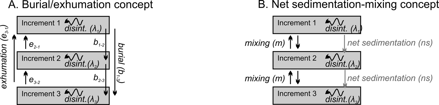
The formation of a time-averaged assemblage of shells and their downcore transit into deeper increments at the base of a mixed layer entails transitions both within (disintegration) and between sedimentary increments (burial, exhumation). A, Three types of transitions—burial (b), exhumation (e), and disintegration (λ, loss from a system)—form the basis of the transition-rate matrices used here to model the formation of time-averaged assemblages. Vertical transitions can be either local (between adjacent increments) or nonlocal (simulating deep callianassid burrowing) and can be increment specific (denoted by subscripts; e.g., higher disintegration rates in shallower increments). All shells enter the column in the top increment at a steady-state rate. B, Assuming that local mixing is symmetric (i.e., an equal probability of upward and downward movements) and that nonlocal mixing is zero, the instantaneous transition rates (in yr−1) can be transformed into the geologically more amenable parameters of mixing (upward and downward movement from bioturbation) and net sedimentation (burial arising from the overall upward movement of the sediment–water interface).
These three parameters can be specific for each increment in a sediment core and can be represented by instantaneous transition rates in a stochastic model formed by the transition-rate matrix (Guttorp Reference Guttorp1995; for details see “Methods”). Individual shells are buried, exhumed, and disintegrate independently in this stochastic model, that is, some subset of shells can move into any deeper increment, some can remain in place, some can move upward into a shallower increment, and others can be lost through disintegration. These models thus apply most clearly to increments affected by biological mixing and other biological processes (bioerosion) that tend to be stochastic, affecting shells individually (Meysman et al. Reference Meysman, Malyuga, Boudreau and Middelburg2008; Aquino et al. Reference Aquino, Roche, Aubeneau, Packman and Bolster2017). Storm- or flood-induced burial–exhumation cycles that act on the entire assemblage (Seilacher Reference Seilacher, Bayer and Seilacher1985; Flessa et al. Reference Flessa, Cutler and Meldahl1993; Sadler Reference Sadler1993; Anderson and McBride Reference Anderson and McBride1996; Katz et al. Reference Katz, Katsman, Kalman and Goodman-Tchernov2022) can also induce some stochasticity: stratigraphically ordered shells are physically reworked (with shells reburied at the base of mobilized sediment) or fine-grained sediment is winnowed (a net upward effect on the positions of shells). Out-of-habitat transport can contribute to shell loss (i.e., the disintegration parameter here) in some settings, but is assumed here to be zero for simplicity.
Figure 1A is the most general quantitative expression of these dynamics in a core that, in this instance, is composed of three sedimentary increments: downward vectors of movement (burial b, which is shell movement into any deeper increment of the sedimentary column either by burrowers or by the addition of new sediment), upward movement (exhumation e, which is shell movement up into any overlying increment, and not necessarily to the sediment–water interface), and disintegration (λ), which removes taxonomically identifiable shells from the system. The vertical movements b and e can represent either local movement between adjacent increments or nonlocal movement between nonadjacent increments (similarly in Trauth Reference Trauth1998; Shull Reference Shull2001; Shull and Yasuda Reference Shull and Yasuda2001; Meysman et al. Reference Meysman, Boudreau and Middelburg2003; Fig. 1A). λ is a function of both the extrinsic taphonomic conditions (including pore water) in a given increment and the intrinsic durability of shells (e.g., size, thickness, organic content, mineralogy).
The burial transition can be expected to exceed the exhumation transition between the two increments schematized in Figure 1A under positive net sedimentation rate, because burial is a composite function of both downward movement by bioturbators and by the addition of new sediment. Various bioturbation regimes that lead to size-selective mixing (e.g., preferential burial of large shells) can also generate differences in burial and exhumation even if net sedimentation is zero. The approach in Figure 1A thus allows that burial and exhumation transitions can differ from each other, can vary with depth downcore, and can represent complicated mixing scenarios with either preferential downward or upward mixing. However, permitting shells to make nonlocal as well as local movements (skipping increments vs. only moving between adjacent increments) increases the number of possible transitions dramatically (e.g., 12 possible transitions given four increments, 20 transitions given five increments, and 30 transitions given six increments), and the transition parameters can be difficult to estimate from AFDs observed in sediment cores.
Figure 1B shows how the number of parameters can be simplified if sedimentation rate is positive, creating a net downward movement of shells. If we assume that the downward (b) and upward (e) transitions of shells induced by mixing alone are set to be equal, and if we then assess those mixing-induced movements across multiple rather than single increments (thus averaging out local differences in burial and exhumation by mixing), then we can convert the analysis to two more mechanistically interesting and geologically measurable types of transitions, namely the net sedimentation rate (ns; the net effect of sediment deposition and erosion on shell position within the sedimentary column) and the between-increment mixing rate of shells (m, with equal upward and downward components) (schematized in Fig. 1B).
Here we focus on this simpler formulation of the dynamics of shell burial (Fig. 1B), exploring the effects of the three key parameters of net sedimentation, biogenic mixing, and disintegration on the time averaging of shell assemblages, and in particular their effects on downcore changes in time averaging. These transition matrices are used as forward models to predict downcore trends in the shapes of AFDs under different combinations (scenarios) of transition parameters. They can also be inverted to estimate these parameters—either burial, exhumation, and disintegration as in Figure 1A or net sedimentation, mixing, and disintegration as in Figure 1B—from the increment-specific AFDs observed in sediment cores (we briefly demonstrate this second application in our “Discussion”). The estimation of parameters and their interpretation is affected by the definition of increment thickness. Increments that are too thick can miss the dynamic of burial and exhumation driven by mixing within increments and/or fail to detect downcore changes in disintegration, whereas increments that are too thin can, for example, exceed the body sizes of shells. Our models implicitly assume that shells typically start their postmortem fate by entering the uppermost (5 cm) increment at the sediment–water interface, for example, as planktic shells settling from the water column, as benthic epifauna inhabiting the sediment–water interface, or as shallow-burrowing infauna. If, owing to a deep infaunal life habit, shells live and die in a deeper, second stratigraphic increment, then that subset of the community can be thought of as contributing to the burial transition between the first and second increments.
Although sedimentary increments tend to be composed of both (taxonomically identifiable) shells and a typically finer clastic sediment (some mix of terrigenous, biogenic, and authigenic grains), we focus here on the fates of individual shells and the emergent, net effects of their transitions on the time averaging of per-increment assemblages encountered downcore. When shells are highly durable and the burial or exhumation transitions induced by burrowers are equal in magnitude and not size selective (i.e., burial and exhumation transitions do not differ between fine matrix and larger shells), then shells in the model are effectively indistinguishable from other sedimentary particles: that is, the sedimentary matrix will have a temporal resolution comparable to that of the shell assemblages. In contrast, when sedimentary particles are subject to size-selective movement (e.g., burrowers such as shrimps preferentially bury coarse particles and exhume fines; Suchanek et al. Reference Suchanek, Colin, McMurtry and Suchanek1986; Wheatcroft and Jumars Reference Wheatcroft and Jumars1987; Tedesco and Wanless Reference Tedesco and Wanless1991; Tedesco and Aller Reference Tedesco and Aller1997; Hupp et al. Reference Hupp, Kelly, Zachos and Bralower2019), then the burial of shells is expected to be significantly faster than their exhumation: transitions that characterize shells would thus be distinct from those characterizing finer sedimentary particles. These transition-rate models thus do not explicitly preserve the mass balance of total sediment (shells and matrix together) per increment—that is, the removal of a shell from an increment does not leave a void that has to be replaced by other shells or sediment.
Relationship of the Transition-Rate Matrices to Earlier Taphonomic Models
Tomašových et al. (Reference Tomašových, Kidwell, Barber and Kaufman2014) modeled the sequestration rate (τ) at which shells transition from a TAZ with high disintegration rate (λ1) into an SZ having a much lower disintegration rate (λ2; λ2 was two orders of magnitude lower than λ1 on the southern California shelf). They modeled and fit this dynamic to surface death assemblages (grab samples of the top 10–15 cm of the seabed). In contrast to our approach here, shells from surface grabs were not partitioned into finer stratigraphic increments. This two-phase exponential model (where the phases refer to two distinct phases of disintegration) directly corresponds to a simple stochastic transition-rate matrix with three transitions—two zone-specific disintegration rates (λ1 and λ2 for the TAZ and the SZ, respectively) and one transition rate (i.e., sequestration, τ) between those two zones. These zones can correspond to two adjacent stratigraphic increments downcore but can also reflect within-increment patches that differ in the degree of bioirrigation and thus in disintegration rates: the two-phase model permits both scenarios.
Mechanistically, the sequestration transition can reflect three mutually nonexclusive pathways by which the shell disintegration rate is reduced. First, shells might accumulate within the TAZ as increasingly old shells because they have encountered refugial microniches or patches with less aggressive pore water (SZs) within a spatially heterogeneous TAZ (actualistic examples in Jørgensen Reference Jørgensen1977; Aller Reference Aller1994; Kristensen Reference Kristensen, Liebezeit, Dittmann and Kröncke2000; Bertics and Ziebis Reference Bertics and Ziebis2010; Lehto et al. Reference Lehto, Glud, á Norði, Zhang and Davison2014). These refuges provide time-outs from disintegration, thus permitting the shell to become older. Second, shells might be sequestered by their simple burial from the TAZ to the underlying SZ, where they also persist because they have achieved a time-out from aggressive, high-disintegration conditions. Obrution models that invoke episodic burial of assemblages by storms or hyperpycnal flows triggered by floods belong to this category of explanations (Seilacher Reference Seilacher, Einsele and Seilacher1982, Reference Seilacher, Bayer and Seilacher1985; Brett et al. Reference Brett, IV, Hunda and Schindler2012), but selective burial by burrowers can be also responsible for moving some shells below the TAZ faster than they would ordinarily become buried. Third, shells located in an SZ—either within the TAZ (pathway 1) or below it (pathway 2)—might have their disintegration rate slowed permanently by diagenetic stabilization, such as via the coarsening of microstructural crystallites (Ostwald ripening; Burdige et al. Reference Burdige, Hu and Zimmerman2010) or via authigenic precipitation of interstitial micrite or micrite envelopes (especially if the residence time in the SZ is long; e.g., Raiswell and Fisher Reference Raiswell and Fisher2004; Tomašových et al. Reference Tomašových, Gallmetzer, Haselmair and Zuschin2022). Such pathways of shell hardening, along with the time-outs provided by temporary burial and advantageous buffering of pore waters by the dissolution of finer carbonate debris (e.g., Walter and Burton Reference Walter and Burton1990), have all been suggested as helping to explain the paradox of preservation of aragonitic shells under prolonged stratigraphic condensation (Kidwell Reference Kidwell1989). Diagenetically stabilized shells (pathway 3) would presumably retain a low, SZ-specific disintegration rate if exhumed back into the TAZ, rather than revert to the high disintegration rates imposed on newly produced shells there. We have suggested that this dynamic of diagenetic stabilization promotes the formation of the heavy-tailed, L-shaped AFDs encountered in the present-day TAZ of the southern California shelf and elsewhere (Tomašových et al. Reference Tomašových, Kidwell, Barber and Kaufman2014).
With three parameters, the transition-rate matrix approach used here and the previous two-phase exponential approach are equivalent. They generate the same parameter estimates when fit to AFDs extracted from the uppermost part of the seabed, such as those captured by a Van Veen grab (i.e., bulk samples that encompass both the TAZ and the SZ, or that penetrate only the TAZ but include shells naturally exhumed into it from a deeper SZ). However, with three parameters only, these approaches do not resolve the pathway of the sequestration transition, nor do they resolve the depth boundary between the TAZ and the SZ—that is, whether shells decrease in their rate of disintegration via a horizontal movement into an SZ microniche or via burial into an underlying SZ, and whether exhumed shells resume high disintegration rates on return to the TAZ, so that the slowdown is strictly transient (as opposed to persistent diagenetic stabilization under SZ conditions). This ambiguity in mechanism can be solved if one shifts from considering the AFD of single bulk sample (our previous approach) to assessing AFDs from two and more stratigraphic increments within the mixed layer. In this latter case, the burial, exhumation, and disintegration rates can be estimated separately for each increment of the mixed layer.
Methods
Transition-Rate Matrices
The transition-rate matrix is arranged so that each row corresponds to the pretransition state of shells in an increment i below the sediment–water interface, and each column represents the state j after the transition occurred. For example, b 1-2 corresponds to the burial rate of a shell from increment 1 to increment 2; e 2-1 corresponds to the exhumation rate of a shell from increment 2 to increment 1 (Fig. 1A); b 1-3 and e 3-1 correspond to nonlocal burial and exhumation rates, respectively; λ1 refers to disintegration rate within increment 1; and λ2 refers to disintegration rate within increment 2 (Fig. 1A). The increments in rows and columns are arranged downcore from the left to the right, and the last row and the last column correspond to the state of disintegration (with the exception of the deepest increment, where the last-column transition corresponds to disintegration and burial into a historic layer). In scenarios where diagenetic stabilization occurs in increments belonging to the SZ (with λ2), shells exhumed from the SZ to the TAZ are not assigned to the state with λ1 but to a new state, here assigned to λexh. In Figure 1B, where burial and exhumation have been converted to a net sedimentation rate (ns) and a between-increment mixing rate (m), the downward movement of a shell from increment 1 to increment 2 is equal to ns + m, and an upward movement from increment 2 to increment 1 is equal to m. This scenario is possible when ns is positive and when bioturbation is on average symmetric with respect to its burial and exhumation components (e.g., sediment mixing does not lead to a preferential burial of coarse particles that would be compensated by exhumation of fines). Nonlocal transitions are thus set to zero in Figure 1B, although when m 1 is high, shells can transit rapidly across several increments. In all forward models used to predict downcore changes in time averaging under various combinations of parameters below, shells enter the death assemblage in the uppermost increment.
Predictions from Forward Models
We predict the shapes of AFDs in each increment, assuming a steady-state input of newly dead shells to the upper increment in a core section with 10 stratigraphic increments, with increment thickness set to 5 cm, thus spanning 50 cm in total thickness (Fig. 2A). The mixing distance and rate at which sedimentary particles are mixed can decline either gradually or abruptly with increasing depth below the sediment–water interface (Swift et al. Reference Swift, Stull, Niedoroda, Reed and Wong1996; Shull Reference Shull2001; Kirtland Turner and Ridgwell Reference Kirtland Turner and Ridgwell2013). The vertical decline in mixing rate has been modeled as an exponential decline (Olszewski Reference Olszewski2004; Steiner et al. Reference Steiner, Lazar, Levi, Tsroya, Pelled, Bookman and Erez2016), a sigmoidal decline (van de Velde and Meysman Reference van de Velde and Meysman2016), and a decline that follows a hyperbolic tangent (Hull et al. Reference Hull, Franks and Norris2011; Kirtland Turner et al. Reference Kirtland Turner, Hull, Kump and Ridgwell2017). These different types of mixing profiles ultimately attempt to mimic high rates of mixing in the uppermost sediment zone that support the highest benthic activity (corresponding to the SML) and subsurface zones that are mixed less frequently (corresponding to the IML; Bentley et al. Reference Bentley, Sheremet and Jaeger2006; Wheatcroft Reference Wheatcroft2006; Ridgwell Reference Ridgwell2007; Meysman et al. Reference Meysman, Malyuga, Boudreau and Middelburg2008, Reference F. J. R., Boudreau and Middelburg2010; Tomašových et al. Reference Tomašových, Kidwell, Alexander and Kaufman2019b). Transition-rate matrices can accommodate the variability in the depth dependency of (1) mixing, (2) disintegration, and (3) whether the shells that are diagenetically stabilized in the SZ retain their high durability (λexh is equal to λ2) when exhumed to the TAZ.
1. We evaluate two types of depth dependency of mixing rate that generate an internally structured mixed layer: (1) mixing rate m 1 declines exponentially from the sediment–water interface to m 2 at the base of the mixed layer (gradual decline in mixing; Fig. 3A), and (2) mixing rate m 1 is relatively high and constant within the upper half of the mixed layer (SML) and abruptly declines to a very small m 2 in the lower half (IML; abrupt decline in mixing; Fig. 3B). m 2 is set to a very small value in all scenarios (0.0001). The base of the entire mixed layer is set at 50 cm, with the SML/IML boundary set at 25 cm in the abrupt-mixing regime (Fig. 2A). We present the predictions for the model with the gradual decline in mixing rate for the scenario with high mixing rate m 1 only because the two mixing regimes do not differ substantially when mixing rate m 1 is low. To explore the effect of increasing mixing depth in the regime having an abrupt decline in mixing rate, we varied the depth of the SML/IML boundary between 5 and 45 cm. We also assessed other versions of the internal structure of the mixed layer, for example, where shells are buried to any increment directly from the uppermost increment (with mixing rates declining toward the base of the mixed layer). We found, however, that the downcore trends in time averaging produced by this more complex version are similar to those of the simplified version specified in Figure 2A.
2. The TAZ (i.e., characterized by relatively high disintegration, λ1) is either (1) limited to the uppermost 5 cm increment of the seabed, that is, the uppermost part of the mixed layer, or (2) extends down to 25 cm (half of the total mixed layer). Disintegration below the TAZ follows λ2, which is set to zero in all scenarios.
3. Shells that are exhumed from the sequestration zone SZ into the TAZ revert to λ1 in a simple model (a reversal model) or acquire λexh that is equivalent to the λ2 that characterized them during their residence in the SZ (diagenetic stabilization model). Diagenetic stabilization of shells and cement precipitation are possible in shallow-subsurface zones where anaerobic degradation of organic matter tends to increase the pH and alkalinity of pore waters (e.g., via sulfate reduction or authigenic methane oxidation; see reviews by Soetaert et al. Reference Soetaert, Hofmann, Middelburg, Meysman and Greenwood2007; Bergmann et al. Reference Bergmann, Grotzinger and Fischer2013), which can lead to an increase in crystal size of the shell surface or micrite precipitation in skeletal pores (e.g., Hover et al. Reference Hover, Walter and Peacor2001; Ge et al. Reference Ge, Pederson, Lokier, Traas, Nehrke, Neuser, Goetschl and Immenhauser2020). Figure 4 visualizes matrices of two scenarios with diagenetic stabilization but otherwise using the same parameters as in scenarios without diagenetic stabilization, including the effect of setting the depth of the TAZ/SZ boundary at 5 cm (Fig. 4A) and at 25 cm (Fig. 4B).
The models used to predict downcore trends in time averaging and to estimate transition parameters from cores as shells transit into deeper increments at the base of a mixed layer, which combines both a surface mixed layer (SML) and a subsurface incompletely mixed layer, IML); movement below the IML, not shown, is into permanently buried historical layers. A, Template for predicting downcore trends in time averaging in a stratigraphic core that has ten 5-cm-thick increments and a total mixed layer characterized by either an abrupt decline (the mixed layer is split into the SML and IML) or a gradual decline in mixing rate (the mixed layer is internally structured but without any obvious break). We use this forward model to predict the shape of age distributions in each increment and thus downcore changes in the time averaging of assemblages across a range of values for the disintegration rate (λ1) in the taphonomically active zone (TAZ; not necessarily equivalent to the SML), the mixing rate within the SML (m 1), the stratigraphic thickness of the TAZ (D TAZ), and net sedimentation (ns), setting the depth of the SML = 25 cm and the depth of the entire mixed layer = 50 cm. Mixing (m 2) in the IML and disintegration rates (λ2) in the sequestration zone (SZ) are both set to zero. Shells exhumed from the SZ to the TAZ disintegrate at λexh, which is set as equivalent to λ2 in the scenario with diagenetic stabilization (i.e., shells do not revert to a rapid λ when exhumed to the SML). B, The transition-rate matrix based on the concept of model B in Fig. 1, which is here fit to shell-age data derived from 10–13 increments in four cores from the southern California continental shelf. This version assumes that mixing rate declines abruptly at the SML/IML boundary and that the TAZ is equivalent to the SML. The gray arrows in A and B represent the diagenetic stabilization scenario, whereby shells exhumed from the SZ to the TAZ possess their own λexh: if λexh is smaller than λ1, that is, shells do not revert to having a high disintegration rate on exhumation back into the TAZ, then diagenetic stabilization is supported.

Two regimes of how mixing rate (1 yr−1) changes with depth. A, A gradual (exponential) decline in mixing rate (values in the legend correspond to the mixing rate in the uppermost 5 cm increment). B, An abrupt decline in mixing rate (with mixing rates remaining the same in the uppermost 25 cm). Total mixed layer thickness is 50 cm and is subdivided into ten 5-cm-thick increments in our model runs; mixing rate declines from the sediment–water interface. Both regimes lead to an internally structured mixed layer, but the regime with the abrupt decline explicitly separates the mixed layer into a surface well-mixed layer (SML) and a subsurface incompletely mixed layer (IML).

The visualization of transition-rate matrices used in predictions of downcore trends in time averaging, with the mixed layer subdivided into ten 5-cm-thick increments (inc.), the surface well-mixed layer (SML) and subsurface incompletely mixed layer (IML) boundary at 25 cm (i.e., the regime with an abrupt decline in mixing rate), and three states that include (1) shells that disintegrate in the taphonomically active zone (TAZ) with rate λ1 (white boxes) and in the sequestration zone (SZ) with rate λ2 (light gray boxes), (2) shells that are exhumed from the SZ to the TAZ and disintegrate in the TAZ with rate λexh = λ2 (gray boxes; diagenetic stabilization, λexh = 0), and (3) shells that were lost by disintegration and/or by burial below the core (dark gray boxes). A, The TAZ/SZ boundary is at 5 cm. B, The TAZ/SZ boundary is at 25 cm. The corresponding transition rates (units are in yr−1) in A and B (units are in yr−1) are based on one scenario, namely with burial in the SML (b 1 = ns + m 1) and in the IML (b 2 = ns + m 2), with exhumation in the SML (e 1 = m 1) and in the IML (e 2 = m 2), and with disintegration in the TAZ (λ1). The R package diagram was used for visualization (Soetaert Reference Soetaert2012).

We note that shell disintegration rate λ may increase with burial (contrary to our assumption that it decreases), for example, if a shell moves downward into a zone of methanogenesis or other conditions promoting loss of organic matrix or demineralization. Shells residing in such sediments would be softened or produce molds and will not survive physical or biogenic reworking back into the TAZ (common shell state in outcrops and some deep cores; e.g., Cherns et al. Reference Cherns, Wheeley and Wright2008; this would be the opposite of diagenetic stabilization). Such a subsurface zone of shell deterioration would either represent the lower part of a TAZ having a complex profile of disintegration or represent a second TAZ located below a shallower subsurface SZ (characterized by very low disintegration). The transition matrices here could be applied to such a dynamic or to one where λ increases downcore, but we do not model those possibilities here. Qualitatively, the effect would be to reduce the potential for increased time averaging in the SML, because exhumation to the sediment–water interface would fail to deliver old shells upward and would act against the development of the right-skewed, L-shaped AFDs that characterize SMLs globally.
We explore downcore trends in the shape of AFDs and in four summary statistics that are widely used in the analysis of time averaging, namely median age, IQR, skewness, and kurtosis. The three parameters that are allowed to vary continuously in our forward models are mixing rate m 1 at the top of the mixed layer (i.e., in the SML), net sedimentation rate (ns), and disintegration rate in the TAZ (λ1), all in expressed in units per year (yr−1). Mixing rates in Figures 1B and 2B refer to 1/time needed to move shells up (to the overlying increment) or down (to the underlying 5-cm-thick increment). Net sedimentation rates refer to 1/time needed to move shells to the underlying 5-cm-thick increment, and thus can be scaled to centimeters/year by multiplying ns by a factor of five, which is the thickness of our increments. If ns = 10, then shells will be moved through the 50-cm-thick mixed layer formed by ten 5-cm-thick increments on average in one time step (1 year). The R scripts that generate transition-rate matrices under different combination of parameters and that visualize the predictions presented in Figures 5–10 are available in Supplements 1–3 (available at https://doi.org/10.5061/dryad.9p8cz8wkz).
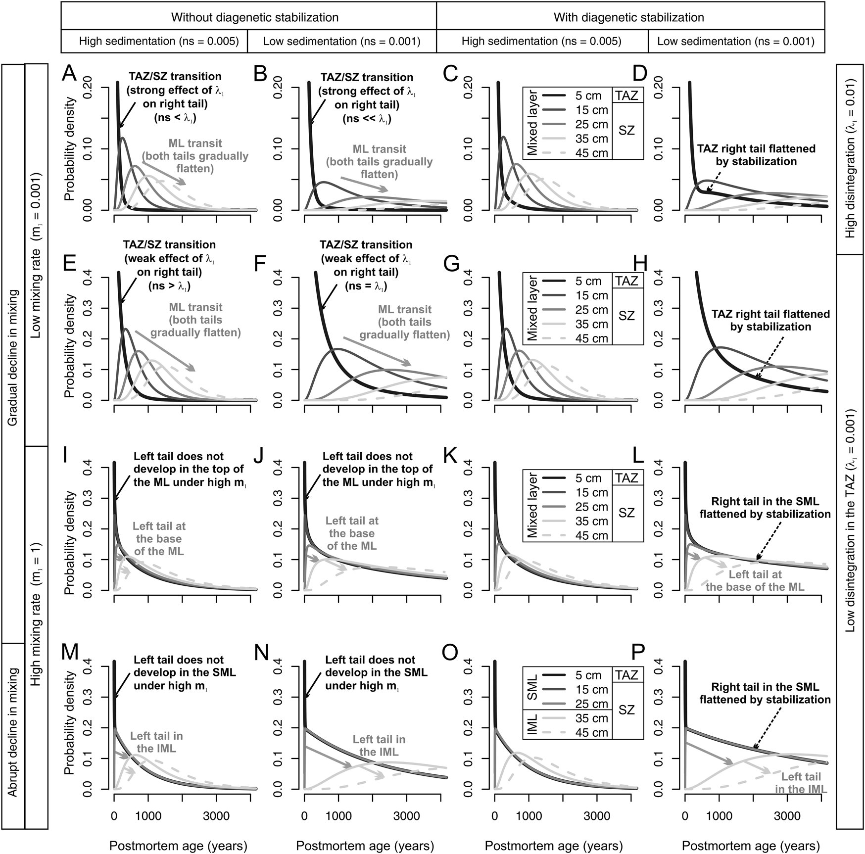
Predicted downcore shift in the shapes of shell age-frequency distributions (AFDs; curves: legend boxes in left column, lighter colors are from deeper increments) within layers affected by stochastic mixing, as a function of two net sedimentation rates (in columns; in 1/yr), under two types of mixing regime (gradual in mixing across 50 cm in A–L or abrupt decline in mixing at 25 cm in M–P), from initially low (A–H) or high mixing rates (I–L), and under scenarios with and without diagenetic stabilization (columns). The taphonomically active zone (TAZ) is limited to the upper 5 cm in all scenarios. A disintegration rate in the TAZ is high in the top row and low in the bottom three rows. All combinations produce a downcore shift from right-skewed to more symmetric age-frequency distributions, with an increase in median age and interquartile age range (IQR) and a decline in skewness and kurtosis. The first shift occurs (the right tail significantly flattens) at the TAZ/sequestration zone (SZ) boundary when λ1 exceeds net sedimentation rate (change from black curves to gray curves; black arrows). The second shift (gray arrows) is characterized by the development of a left tail (and further right-tail flattening) and develops through the entire mixed layer when mixing rate m 1 is low, or in only the lower parts of the mixed layer (in the gradual-decline regime) or at the surface well-mixed layer (SML) and subsurface incompletely mixed layer (IML) boundary (in the abrupt-decline regime) when mixing rate m 1 is high. In scenarios with diagenetic stabilization, time averaging of assemblages in the upper part of the mixed layer increases significantly by the inclusion of shells exhumed from the SZ to the TAZ. These old shells, which persist in the TAZ despite the high disintegration rates that apply to newly produced shells there, flatten and extend the right tail of the AFDs in the SML, producing L-shaped distributions. ML, mixed layer.
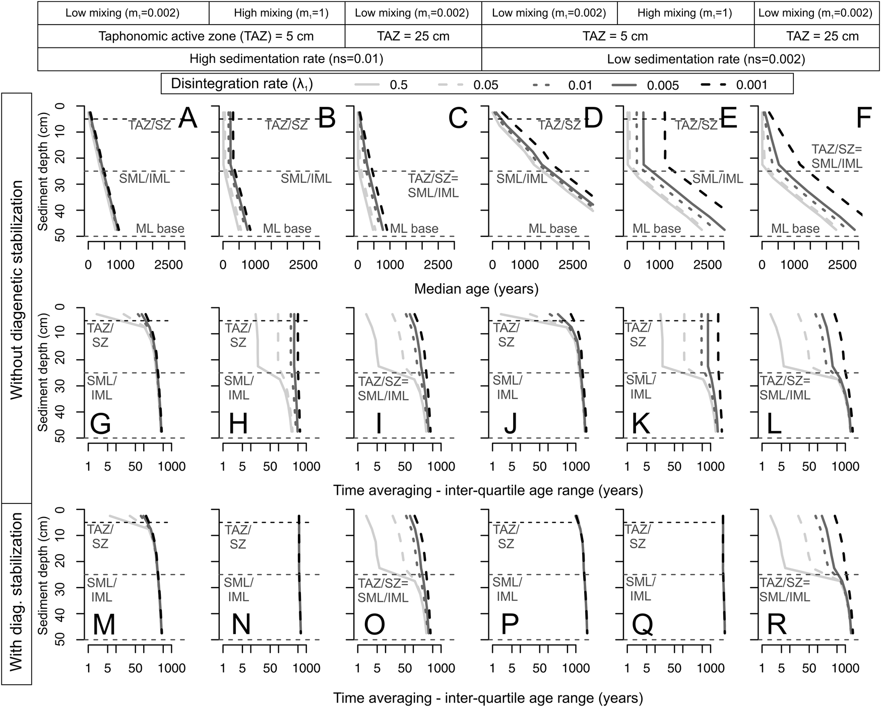
Predicted downcore changes (sediment depth, vertical axes) in median age (A–F) and time averaging (IQR, in G–R) as a function of net sedimentation rate (curves; darker colors are slower) under an abrupt decline in mixing rate at 25 cm, with both low and high disintegration rates in the taphonomically active zone (TAZ; λ1, columns), with two different TAZ depths set at either 5 cm or 25 cm downcore (columns), and with both low and high mixing rate (m 1, columns). The scenarios without diagenetic stabilization are shown in the upper two rows (A–L, units of all rates are in yr−1), and the scenarios with diagenetic stabilization are shown in the bottom row (M–R). Median age increases downcore in all scenarios, but the increase is strongest when net sedimentation rate is slow. All scenarios show a downcore increase in time averaging (IQR), except when the mixing rate through the entire mixed layer is high, homogenizing shell ages (H, K, N, Q). The effect of diagenetic stabilization, that is, where shells exhumed from the sequestration zone (SZ) to the TAZ retain a very low λ2, is to increase IQR at all depths relative to models where exhumed shells revert to a high disintegration rate; it can also set IQR at a high value throughout the entire mixed layer (M–R). Note that the x-axis in the plots with IQR has a logarithmic scale. Dashed black horizontal lines denote the TAZ/SZ boundary (set at either 5 cm or 25 cm), and dashed gray horizontal lines denote both the surface well-mixed layer (SML) and subsurface incompletely mixed layer (IML) boundary at 25 cm and the base of the entire mixed layer (ML).

Predicted downcore changes in median age (A–F) and time averaging (interquartile age range [IQR], in G–R) as a function of disintegration rate (λ1) in the taphonomically active zone (TAZ; curves; darker colors are lower rates; depth of TAZ set at either 5 cm or 25 cm downcore) under an abrupt decline in mixing rate at 25 cm, with both low and high net sedimentation rate (ns) and both low and high mixing rate (m 1). The scenarios without diagenetic stabilization are shown in the upper two rows (A–L, units of all rates are in yr−1) and the scenarios with diagenetic stabilization are shown in the bottom row (M–R). Median ages increase downcore under all scenarios, except where m 1 is very high, which produces a homogeneous IQR within the surface well-mixed layer (SML). Higher λ1 results in less time averaging in the SML (also relevant for fragile shells in the assemblage compared with durable shells). However, the effect of λ1 on IQR diminishes in the subsurface incompletely mixed layer (IML), where IQRs converge to the same value, regardless of λ1 in the TAZ. In scenarios with diagenetic stabilization (M–R), IQRs also decline downcore in all scenarios, with the exception of conditions with high mixing rate m 1. ML, mixed layer.
In scenarios with relatively high disintegration rate (λ1 = 0.01 yr−1) and a mixing rate (m 1 = 0.002 yr−1) that does not exceed net sedimentation rate (ns = 0.002 yr−1), with the surface well-mixed layer (SML) and subsurface incompletely mixed layer (IML) boundary at 25 cm, the peak in skewness and kurtosis of age distributions occurs at the base of the taphonomically active zone (TAZ) rather than in the uppermost increment. The downcore increase in the depth of the TAZ/sequestration zone (SZ) boundary, from 5 cm (light gray) to 45 cm (dark gray), is thus associated with a downward shift in the location of age-frequency distributions (AFDs) characterized by a highly positive skewness and kurtosis, which is driven by exhumation of old shells from the SZ to the base of TAZ, where they are then mixed with rapidly disintegrating (and thus young) shells.

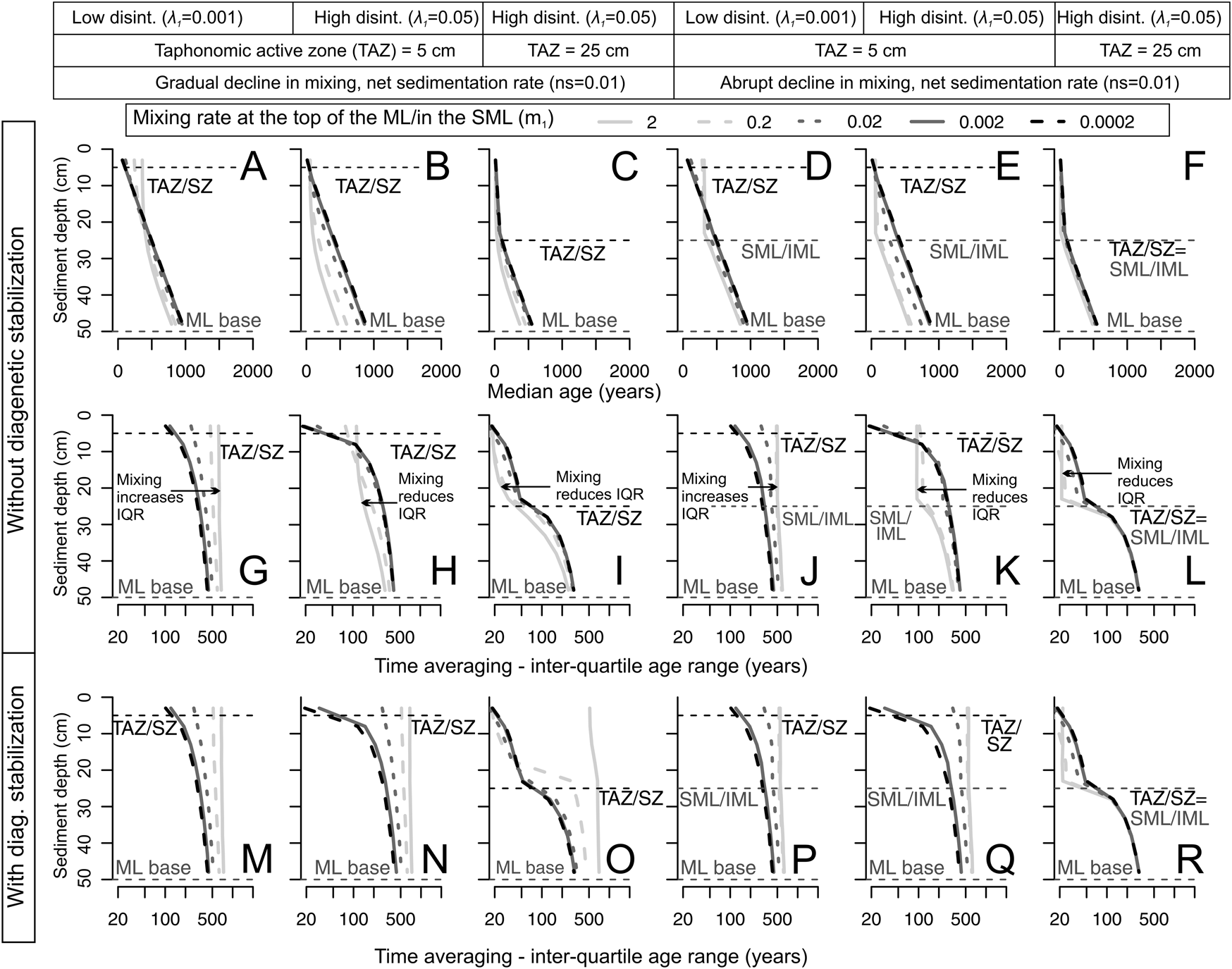
Predicted downcore changes in median age (A–F) and time averaging (interquartile age range [IQR]) as a function of mixing rate m 1 (curves; darker colors are lower rates) in the top of the mixed layer (gradual decline in m 1) or in the surface well-mixed layer (SML; abrupt decline in m 1), under both high (λ1 = 0.05) and low disintegration rates (λ1 = 0.001) within the taphonomically active zone (TAZ; thickness set at either 5 cm or 25 cm depth downcore) and with high net sedimentation rates (ns = 0.01). A low m 1 under a regime of gradually declining mixing rate (A–C) is required to produce a downcore increase in median age, whereas any mixing rate can produce it under a regime with an abrupt decline in mixing (D–F). These scenarios show that, when disintegration rates are low in the TAZ (top 5 cm), high mixing rates result in higher time averaging in the upper part of the mixed layer regardless of mixing regime (G, J). When disintegration rates are high in scenarios without diagenetic stabilization (G–L), high mixing rates have the opposite effect, that is, they reduce time averaging (IQR) in the mixed layer, because shells are recycled back into the TAZ, where they disintegrate (H, K). When the TAZ depth increases from 5 to 25 cm, time averaging (IQR) is further reduced (I, L): shells spend more time within the TAZ before reaching a time-out within the sequestration zone (SZ). Diagenetic stabilization (M–R) simplifies the interaction between λ1 and m 1 so that IQR increases with increasing mixing rate m 1in all scenarios.
Predicted downcore changes in median age (A–F) and time-averaging (interquartile age range [IQR], in G–R) in scenarios with an abrupt decline in mixing rate in the SML but permitting the depth of the surface well-mixed layer (SML) to increase from 5 cm to 45 cm (curves; dark colors are deeper SML), under both high (ns = 0.01) and low net sedimentation rate (ns = 0.002) and under both low (λ1 = 0.001) and high disintegration rates (λ1 = 0.01), with the depth of the taphonomically active zone (TAZ) equal to either 5 cm or 25 cm; mixing rate is high in all scenarios (m 1 = 1). All scenarios both without (G–L) and with diagenetic stabilization (M–R) produce a downcore increase in IQR. The effect of the SML depth on IQR is modulated significantly by λ1 (bottom row): when disintegration is low (or net sedimentation is high), then increasing the SML depth increases IQR, whereas when disintegration is high (or net sedimentation is low), then increasing the SML depth reduces IQR. In the scenarios with diagenetic stabilization, the effect of λ1 on IQR diminishes, and any increase in the depth of the SML will increase IQR.

Estimating Transition-Rate Parameters from AFDs Observed in Cores with Inverse Models
To estimate parameters in Figure 2 from empirical AFDs collected from successive core increments using transition-rate matrices, the maximum likelihood estimator can be used to estimate the vector Θ transition parameters with the C increments (11–13 increments in cores from the southern California shelf) and the K states. In models without diagenetic stabilization, K refers to the number of increments (all increments that can be directly observed in cores) plus the last state K, which is represented by disintegration. This last state is latent, that is, unobservable. In models with diagenetic stabilization, the TAZ increments that receive shells from the SZ are characterized by two latent states, that is, the disintegration of shells that were not buried to the SZ and the disintegration of shells exhumed from the SZ (Fig. 4). The transition matrix has the form A(Θ) = Q(Θ)D(Θ)Q −1(Θ), describing the rate as a continuous-time Markov chain that moves between states. We assume that the starting state is 1 in the uppermost increment and that other states are initially zero (i.e., dead shells only enter the uppermost increment and are missing in the subsurface increments). We thus have an initial probability vector μ = (1, 0, …0) and the probability vector at time t will be μ exp(tA(Θ)) = μQ(Θ)exp (tD(Θ))Q −1(Θ). This will lead to the following log-likelihood function if we can observe all states:
 $$ \eqalign{& {\rm log}L ( {\rm \Theta } ) = \mathop \sum \limits_{i = 1}^n {\rm log} \boldsymbolgg [ {\mathop \sum \limits_{k = 1}^K \mathop \sum \limits_{\,j = 1}^K Q_{1j} ( {\rm \Theta } ) \exp } \cr & { { {t_i{\rm \lambda }_j ( {\rm \Theta } ) } } Q_{\,jk}^{{-}1} ( {\rm \Theta } ) I ( {c_i = k} ) } \boldsymbolgg] \cr & - n{\rm log} \boldsymbolgg[ {-\mathop \sum \limits_{j = 1}^{K-1} Q_{1j} ( {\rm \Theta } ) {\rm \lambda }_j^{{-}1} ( {\rm \Theta } ) \mathop \sum \limits_{k = 1}^{K-1} Q_{jk}^{{-}1} ( {\rm \Theta } ) } \boldsymbolgg ]}$$
where λj(Θ) is the jth eigen value of A(Θ). When the observed state category is different from the latent state, we denote B as an L by K matrix that matches each K latent state to a L potential observable, that is, B ij = 1 if and only if latent state i belongs to observable state j. In this case, the log likelihood for the observed states will be:
 $$ \eqalign{& {\rm log}L ( {\rm \Theta } ) = \mathop \sum \limits_{i = 1}^n {\rm log} \boldsymbolgg [ {\mathop \sum \limits_{l = 1}^L \mathop \sum \limits_{k = 1}^K \mathop \sum \limits_{\,j = 1}^K Q_{1j} ( {\rm \Theta } ) {\rm exp} }\cr &{ { {t_i{\rm \lambda }_j ( {\rm \Theta } ) } } Q_{\,jk}^{{-}1} ( {\rm \Theta } ) B_{lk}I ( {\widetilde{{c_i}} = l} ) \boldsymbolgg ] }\cr& { -\, n{\rm log}} \boldsymbolgg [-\mathop \sum \limits_{\,j = 1}^{K-1} Q_{1j} ( {\rm \Theta } ) {\rm \lambda }_j^{{-}1} ( {\rm \Theta } ) \mathop \sum \limits_{k = 1}^{K-1} Q_{\,jk}^{{-}1} ( {\rm \Theta } ) \boldsymbolgg ] $$
We use the quasi-Newton method to solve this optimization problem and get estimates of model parameters for Θ on the basis of age data from four cores from southern California (Fig. 2B). The R language scripts for these inverse models that fit the matrices to sediment cores using maximum likelihood are available in Supplements 4–6 (available at https://doi.org/10.5061/dryad.9p8cz8wkz).
Sediment Cores and Model Evaluation
We collected multiple 50 × 50 cm boxcores and 8-cm-diameter vibracores at four sites in 2012 on the Palos Verdes and San Pedro shelves of southern California (Los Angeles and Orange Counties; Supplementary Table S1). The depositional conditions and benthic ecosystems at both shelves were affected by wastewater outfalls that opened in the early twentieth century (Stull et al. Reference Stull, Haydock, Smith and Montagne1986, Reference Stull, Swift and Niedoroda1996; McGann Reference McGann2009). Two sites are located in 50 m water depth outside the area of solid-sediment effluent-layer deposition on the Palos Verdes (PVL10-50; Leonard-Pingel et al. Reference Leonard-Pingel, Kidwell, Tomašových, Alexander and Cadien2019) and San Pedro shelves (OC-50; Tomašových et al. Reference Tomašových, Kidwell, Alexander and Kaufman2019b), with relatively low rates of sedimentation in the twentieth century (<0.1–0.2 cm/yr; Tomašových et al. Reference Tomašových, Kidwell, Alexander and Kaufman2019b). The other two sites (PVL5-50 and PVL5-75) are located in 50 and 75 m water depth on the Palos Verdes shelf within the effluent layer sourced from the White Point outfall, with the twentieth-century sedimentation rates attaining ~1 cm/yr (Eganhouse and Pontolillo Reference Eganhouse and Pontolillo2000; Santschi et al. Reference Santschi, Guo, Asbill, Allison, Kepple and Wen2001; Lee et al. Reference Lee, Sherwood, Drake, Edwards, Wong and Hamer2002).
AFDs are based on pooling the shell ages of two infaunal aragonitic bivalves (Nuculana taphria and Parvilucina tenuisculpta) estimated using amino acid racemization (AAR) calibrated to 14C. Shell ages from the low-sedimentation-rate sites PVL10-50 and OC-50 were published in Tomašových et al. (Reference Tomašových, Kidwell, Alexander and Kaufman2019b), and those from the high-sedimentation rate sites PVL5-50 and PVL5-70 were estimated using the same species-specific 14C-amino acid calibrations and are published here (Supplement 7 available at https://doi.org/10.5061/dryad.9p8cz8wkz). The two species represent the most common species in molluscan death assemblages at these four sites. Shell ages of both species were pooled into increment-specific AFDs in order to damp the effects of temporal changes in shell production (N. taphria had low population densities during peak mid–twentieth century wastewater when P. tenuisculpta had high densities; Tomašových et al. Reference Tomašových, Kidwell and Barber2016). All cores were initially split to 2-cm-thick increments. We analyze shells pooled into 4- to 5-cm-thick increments covering 55 cm of core (upper 13 increments) at the low-sedimentation sites outside effluent deposition (PVL10-50 and OC-50), and from 4- to 5-cm-thick increments in the upper 40 cm and ~10-cm-thick increments below (covering 100–150 cm) at the high-sedimentation sites within effluent deposition at PVL5-50 (13 increments) and PVL5-75 (11 increments, Supplementary Table S2). Numbers of shells per increment exceeded 50–100 at PVL10-50 and OC-50, and so the AAR-dated shells there represent random subsets of ~50 shells from the Nuculana and Parvilucina assemblages (shell ages published in Tomašových et al. Reference Tomašových, Kidwell, Alexander and Kaufman2019b). Sample sizes were smaller in the cores from PVL5-50 and PVL5-75 at core depths >40 cm, because these deeper increments were not captured by boxcores at these sites, only by vibracores, and thus age distributions are based on all shells collected.
The IQR of each incremental AFD—widely used to quantify time averaging—is corrected for the calibration error using a new method suggested to us by Thomas D. Olszewski (personal communication 2022). Previous methods of correction have assumed that the error-corrected estimate of the IQR can be approximated by subtracting the error component of the IQR from the raw IQR (e.g., Dominguez et al. Reference Dominguez, Kosnik, Allen, Hua, Jacob, Kaufman and Whitacre2016; Tomašových et al. Reference Tomašových, Kidwell, Alexander and Kaufman2019b). Here, we rely on additive partitioning of the total age variance (such as observed in each AFD), which can be decomposed into the true (error-corrected) variance and the variance generated by the calibration error. Using this approach, the squared standard deviation produced by the calibration error alone is first subtracted from the squared total standard deviation of each increment-specific AFD. The square root of this value corresponds to the error-corrected standard deviation. Second, this error-corrected standard deviation is then translated for each AFD into an error-corrected IQR using the observed ratio of the raw standard deviation to the raw IQR of that AFD (Figure S6).
Five parameters (λ1, λ2, m 1, m 2, ns), using a model with the abrupt decline in mixing rate between the SML and the IML, are fit to AFDs in each of the four sediment cores: AFDs correspond to 11–13 increments ranging from 4 to 10 cm thick, with increments split into the SML with λ1 and m 1 and the IML with λ2 and m 2 (Fig. 2B). The depth of the SML is estimated on the basis of the thickness of the uppermost vertical or steep (steeper than expected on the basis of net sedimentation rate) segments of the profile in the excess 210Pb activity. We then assess whether the parameters estimated by fitting can reproduce the downcore trends in IQR, median, skewness, and kurtosis observed in sediment cores. The depth of the SML is set to 25 cm at PVL10-50 and to 20 cm at OC-50 where this unit corresponds to a layer with abundant fish scales and worm tubes; this is comparable to the depths of active bioturbation observed at these water depths on the Palos Verdes shelf in the 1990s (Swift et al. Reference Swift, Stull, Niedoroda, Reed and Wong1996; Niedoroda et al. Reference Niedoroda, Swift, Reed and Stull1996). The depth of the SML is set to 40 cm at PVL5-50 and PVL5-75: this subdivision is approximate, because the two effluent sites differ in the degree of mixing in the upper 40 cm based on 210Pb, with uniform ages at PVL5-50 and monotonically increasing ages at PVL5-75.
Results
Predicted Downcore Shifts in the Shapes of AFDs
Within the 50-cm-thick mixed layer, where the depth of the TAZ is set at 5 cm, both the gradual- and abrupt-change mixing regimes produce a downcore shift in the shapes of age distributions, specifically a downcore increase in both median age and IQR, accompanied by a decrease in skewness and kurtosis (Fig. 5). When mixing rate m 1 is low and there is no diagenetic stabilization in the SZ (Fig. 5A,B,I,J), the change in AFD shape is concentrated at two depths. The first change is at the TAZ/SZ boundary: the right tail significantly flattens when disintegration rate λ1 in the TAZ exceeds net sedimentation rate and declines below the TAZ (black arrows in Fig. 5A,B). This sharp change is thus especially visible where net sedimentation rate is low. The second change occurs at the point when the left tail develops at sediment depths that are beyond the reach of rapid burial of the youngest shells by burrowers, which is below the TAZ in the lower part of the mixed layer (or in the IML). This dynamic leads to a downcore succession of AFDs with gradually increasing IQR and declining skewness and kurtosis as shells pass through the whole mixed layer (Fig. 5E,F). The development of the left tail and the flattening of the right tail are pronounced when net sedimentation rate is low. Even when the forward models used to predict downcore changes in Figures 5–10 permit only local transitions between adjacent increments, stochasticity in that between-increment mixing permits some subset of shells to pass quickly among increments so that they can be rapidly buried. That process of burial is further accelerated when nonlocal transitions are allowed.
When mixing rate m 1 is high and shells are not diagenetically stabilized (Fig. 5I,J,M,N), AFDs without any left tail extend more deeply into the mixed layer owing to rapid downward mixing of young shells. All increments within the well-mixed SML, including the uppermost 5 cm that constitutes the TAZ, are thus dominated by young cohorts (Fig. 5I,J,M,N), in contrast to lower mixing rates that promote such AFDs only within the TAZ (Fig. 5A,B,E,F). Under high mixing, the right tail of AFDs in the upper 25 cm is steep and determined by disintegration, because it is limited to shells that have not disintegrated while residing within the SML, rather than being fed by much older shells that have been exhumed from deeper increments. Therefore, AFDs develop the left tail in deeper increments at the base of the mixed layer in the gradual-decline regime (Fig. 5I,J) or at the SML/IML boundary in the abrupt-decline regime (Fig. 5M,N). Similarly to regimes with low mixing rate, the downcore flattening of AFDs is most pronounced when net sedimentation rate is low.
When the model permits diagenetic stabilization to occur in the SZ and sedimentation rate is high, then the downcore progression of AFDs is similar to that of scenarios without diagenetic stabilization (Fig. 5C,G,K,O): old, stabilized shells in the SZ have low likelihood of exhumation back up into the TAZ. However, when diagenetic stabilization occurs and sedimentation rate is low, allowing very old shells to remain within the reach of deep mixing, then L-shaped distributions can be produced in the TAZ: diagenetic stabilization means that shells exhumed to the TAZ retain a very low, SZ-specific disintegration even after exhumation (λexh = λ2), that is, shells are inert. This process flattens the right tail of the AFD within the TAZ (black dashed arrows in Fig. 5D,H,L,P). These AFDs do not have any left tail, because they are located in the uppermost increment, which experiences a steady-state input of young shells. Despite the right-skewing effect of diagenetic stabilization on AFDs in the uppermost increments, the IQRs there are still smaller than in deeper increments: IQRs increase and skewness and kurtosis decline in subsurface increments within the mixed layer (Fig. 5D,H,L,P).
Predicted Effects of Net Sedimentation Alone
All scenarios—sedimentation rate is constant over the duration of deposition, but differs among scenarios—show a monotonic downcore increase in the median age of shells (top row in Fig. 6) except where the mixing rate is high, which leads to an age-homogeneous SML; median age then increases progressively through only the deeper part of the mixed layer (IML; Fig. 6B,E, Supplementary Fig. S1). Decreasing the net sedimentation rate increases IQR in all increments within the mixed layer, regardless of mixing regime, because slower sedimentation slows the transit time of shells to deeper increments; this result is true both with and without diagenetic stabilization (middle and bottom rows in Fig. 6). Notably, a low sedimentation rate does not always lead to high IQR in the SML (Fig. 6I, Supplementary Fig. S1) if (1) the TAZ is deep and the disintegration rate in the TAZ (λ1) is higher than the net sedimentation rate by which shells are buried below the TAZ (i.e., the rate of disintegration is greater than the rate of burial induced by new sediment deposition); and (2) there is no diagenetic stabilization (in Fig. 6G–L): IQR increases and skewness and kurtosis decline downcore (Supplementary Fig. S2), unless mixing rate m 1 is very high. In scenarios with diagenetic stabilization (Fig. 6M–R), IQR is higher in comparison to counterpart scenarios without diagenetic stabilization under all mixing regimes (particularly in the IML) but is less affected in the parts below the IML/SML interface. When the TAZ is as deep as the SML, few shells are exhumed from the SZ to the SML, and the effect of diagenetic stabilization on IQR is thus minor (Fig. 6O,R).
Predicted Effects of Disintegration within the TAZ and of the Depth of the TAZ
An increase in disintegration within the TAZ (λ1) and/or an increase in the depth of the TAZ reduces IQRs in the TAZ (curves in Fig. 7, Supplementary Fig. S3), especially when λ1 is high relative to net sedimentation rate (i.e., shells disintegrate before they can age). The downcore increase in IQR and the decline in skewness and kurtosis is stronger when λ1 is high, because the decline in disintegration from λ1 to λ2 at the TAZ/SZ boundary is especially strong (curves in Fig. 7G,J, Supplementary Fig. S4). When mixing rate m 1 is low, the downcore decline in IQR occurs at the TAZ/SZ boundary (Fig. 7G,J); when mixing m 1 is high in the SML, then the shift in the shape of AFDs occurs at the SML/IML boundary (Fig. 7H,K). The difference in IQR between low (e.g., λ1 = 0.5) and high disintegration (e.g., λ1 = 0.001) regimes in the TAZ is smaller in the SZ, and when mixing m 1 is high, this convergence occurs in the IML or at the base of the ML (lines converge in the lower parts of the mixed layer in Fig. 7G–L). Therefore, the slope of the right tails of AFDs below the TAZ is determined more by burial induced by mixing and by new sedimentation than by disintegration. When diagenetic stabilization occurs and the depth of the SML exceeds the depth of the TAZ, the downcore increase in IQR is mild (Fig. 7M,N,P,Q): shells exhumed from the SZ to the TAZ converge to the same values of SZ-specific disintegration (λexh = λ2) and thus increase IQR in the whole mixed layer.
In scenarios having a deep TAZ (at 25 cm) that coincides with the SML/IML boundary and subject to slow mixing m 1 (both with and without diagenetic stabilization), the usual downcore decline in skewness and kurtosis can be interrupted by a conspicuous peak, with strongly right-skewed and leptokurtic AFDs occurring just at the base of the TAZ (Supplementary Fig. S4). The deepening of this peak shifts in parallel with the deepening of the TAZ (Fig. 8). This outcome is typical of scenarios with a very slow mixing rate. Under those conditions, very old shells that are exhumed from the underlying SZ to the base of the TAZ either (1) are transient, that is, their time to disintegration is shorter than their time to exhumation to higher increments, and/or (2) persist in the TAZ because they have been diagenetically stabilized, but their rate of exhumation to the sediment–water interface is still lower than net sedimentation rate. These subsurface AFDs are heavy-tailed on the right, but they have also a left tail produced by slow mixing-induced downward burial of young shells, in contrast to the L-shaped distributions occurring in the surface AFDs.
The differences in the downcore trajectories in median age and IQR created by different disintegration rates (Fig. 7) can be read as the trajectories of fragile as opposed to durable shells within a single assemblage. In scenarios without diagenetic stabilization, median ages in the TAZ are smaller under high disintegration rates than under low disintegration, which is comparable to fragile shells having smaller median ages than durable shells within any sedimentary increment. This effect also propagates downward below the TAZ: more fragile shells are younger than more durable shells within the same increment (Fig. 7A–F). However, the effect of disintegration rate on median age in the lower increments of the mixed layer is diminished under conditions of high sedimentation rate (all shells are more likely to be buried before disintegration occurs) and low mixing rate (Fig. 7A compared with B–F).
Predicted Effects of Mixing Rate and Mixing Depth
In scenarios where the TAZ disintegration λ1 is low, an increase in mixing rate m 1 (curves in Fig. 9G,J) and/or an increase in the depth of the SML (curves in Fig. 10G,J) increases time averaging at all sediment depths within the mixed layer, because a subset of older shells that would ordinarily be buried into historic layers remain longer within the mixed layer. In contrast, when λ1 is high, an increase in mixing rate m 1 (curves in Fig. 9H,I,K,L) or in the depth of the SML (curves in Fig. 10I,K,L) reduces IQR, because shells are perpetually exhumed back to the TAZ where they experience high disintegration (in scenarios without diagenetic stabilization). Even when the TAZ/SZ boundary lies above the SML/IML boundary, shells in SZ increments are not protected from disintegration, because they cycle rapidly back into the TAZ. High mixing rates can thus reduce IQR throughout the mixed layer. Such mixing prolongs the total residence time of shells in the TAZ, even if that residence is intermittent. This covariation is expected if, for example, high mixing rates and deep mixing directly enhance bioirrigation and thus disintegration by intensifying aerobic organic matter degradation.
In scenarios where the mixing rate m 1 is low (darker curves in Fig. 9), shells that are initially mixed downward and/or bypass the TAZ are less likely to return back to the TAZ, creating a more monotonic downcore increase in median age and also increasing IQR in the lower parts of the mixed layer. Therefore, the ability of high λ1 to decrease IQR in the mixed layer disappears as m 1 slows, assuming no diagenetic stabilization, even when the mixed layer is deep (Fig. 10): shells that lie below the TAZ but still within the SML are less likely to be exhumed back to the TAZ. In the scenarios with diagenetic stabilization, we find that the exhumation of older shells from the SZ into the TAZ cancels the interaction between λ1 and the mixing rate m 1 (Fig. 8G–Q): this interaction disappears because λexh of the exhumed shells corresponds to the low λ2 of the SZ. For the same reason, diagenetic stabilization also cancels the interaction between λ1 and the depth of the mixed layer (Fig. 9G–Q).
Observed and Modeled Downcore Trends in AFDs on the California Shelf
Although our primary aim is to explore the theoretical phase space of effects of mixing, sedimentation, and disintegration on time averaging, the power of the model can be assessed by comparing its predicted downcore trends against those observed in the field, using cores from southern California to estimate model parameters.
The four cores exhibit a similar trajectory in median age (Fig. 11), with a relatively age-homogeneous SML that is 20–25 cm thick at the two low-sedimentation, non-effluent sites (PVL10-50 and OC-50), and is 40 cm thick at the two high-sedimentation, effluent-affected sites (PVL5-50 and PVL5-75). Median age within the SML decreases with increasing sedimentation rate: it varies between ~200 and 800 years at PVL10-50, between ~100 and 200 years at OC-50 (low-sedimentation sites), and between ~20 and 100 years at the high-sedimentation PVL5-50; the median age increases gradually within the upper 40 cm from 10 to ~90 years at the second high-sedimentation site, PVL5-75. The SMLs at the low-sedimentation sites are composed of shell-poor muddy sand. They are underlain by a shell bed at ~20–40 cm (median age ~2000–5000 years). In contrast, at the high-sedimentation sites, the shell beds are represented by (isochronous) shell-poor sandy muds, and these muds occur 40–60 cm lower in the core. The median age increases to ~10,000 years at 60 cm and 100 cm at the low-sedimentation sites (PVL10-50 and OC-50, respectively), and increases to only ~3000–4000 years at 150–170 cm at the high-sedimentation sites (PVL5-50 and PVL5-75).
Modeled downcore trends in median age and interquartile age range (IQR; produced by estimating parameters on the basis of age data in four cores using Fig. 2B) compared with the observed trends in the age-frequency distributions (AFDs) of assemblages that combine two aragonitic infaunal bivalve species in four sediment cores on the southern California shelf that differ in net sedimentation rates (estimates in cm/yr on the left refer to the twentieth-century sedimentation rates). At each site, the models predict downcore increases in median age and IQR that generally agree with trends observed in cores, despite dramatically different rates of net sedimentation among sites; black lines with a darkly shaded confidence interval correspond to a model without diagenetic stabilization, and gray lines with a lightly shaded confidence interval correspond to a model with diagenetic stabilization. The gray sector in the uppermost parts of cores corresponds to the surface mixed layer (SML) as indicated by 210Pb analysis and characterized by uniform shelliness and grain size (Supplementary Table S1). The observed IQR is corrected for age error induced by the calibration of amino acid racemization values by 14C; dashed lines correspond to 95% confidence intervals.
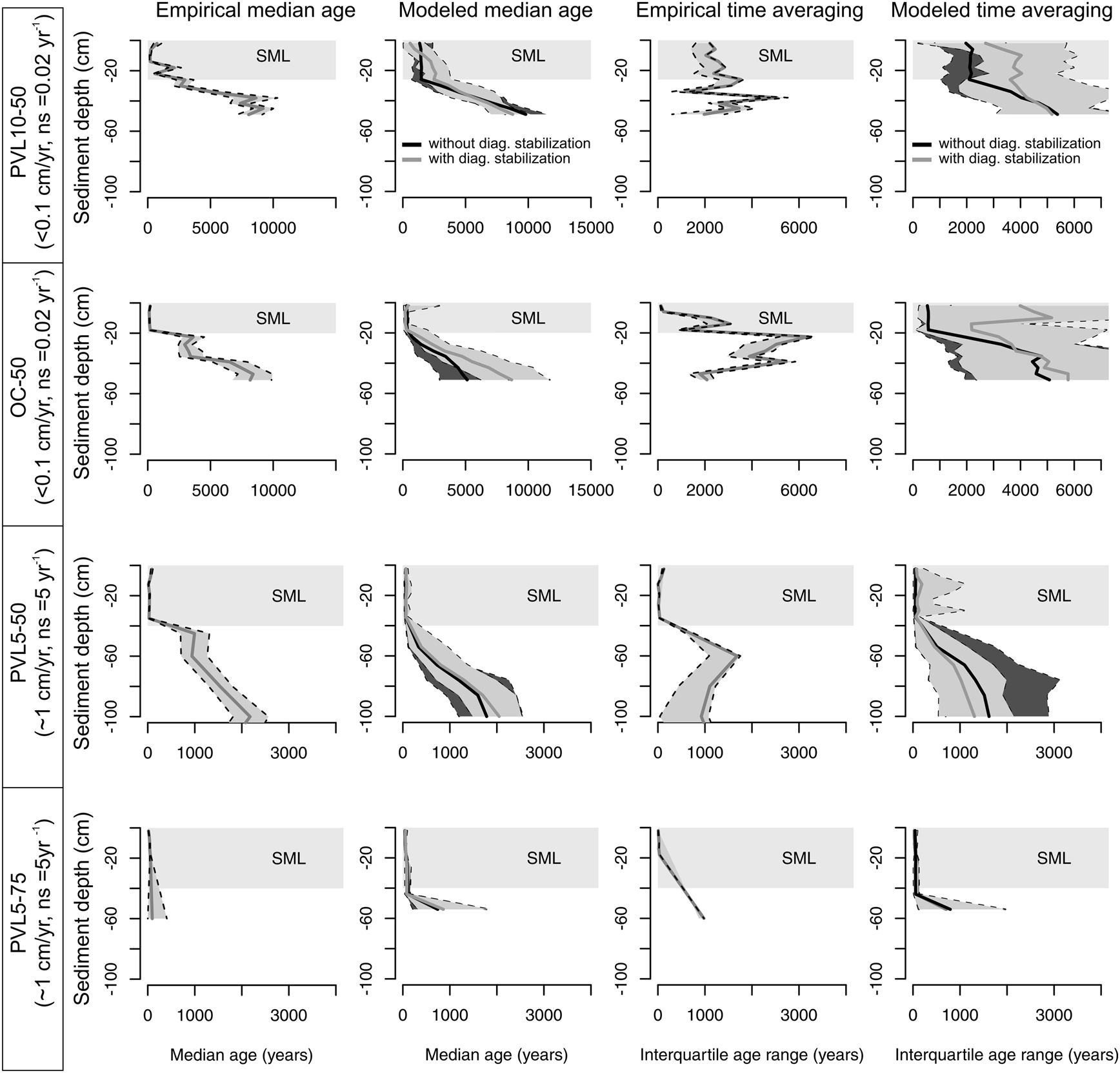
IQR exhibits a strong downcore increase from centennial to millennial scales at all sites except one of the low-sedimentation sites (PVL10-50), where it increases between the SML and the subsurface shell bed (from ~2000 years in the SML to variable IQR ranging between 2000 and 5000 years in the subsurface; Fig. 11). The per-increment IQR increases modestly from 130–3000 years in the SML to 2000–5500 years in the IML at the other low-sedimentation site (OC-50). In contrast, the per-increment IQR at the high-sedimentation sites increases from 10–120 years in the SML to 700–1000 years in the IML (PVL5-50) and from 10–30 years in the SML to ~1000 years in the IML (PVL5-75), that is, by one to two orders of magnitude. All sites exhibit a decline in skewness and kurtosis (Fig. 12), with AFDs shifting downcore from right-skewed to more symmetric and flatter distributions.
Modeled and observed downcore trends in skewness and kurtosis of shell age-frequency distributions (AFDs), as in Fig. 11. Modeled trends are produced by estimating parameters based on the four sediment cores, as shown in Fig. 2B. Both skewness and kurtosis tend to decline downcore in cores and in models (black lines with a darkly shaded confidence interval correspond to a model without diagenetic stabilization with five parameters, and gray lines with a lightly shaded confidence interval correspond to a model with diagenetic stabilization and thus six parameters). Dashed lines correspond to bootstrapped 95% confidence intervals on observed values.

Simple models that use our transition matrix approach and assign increments in each core into an SML and IML a priori, with the five parameters (ns, m 1, m 2, λ1, λ2) fit to the sediment core data (Supplementary Table S3), do a good job of replicating observed downcore increases in median age and IQR (Fig. 11) and declines in skewness and kurtosis (Fig. 12, Supplementary Table S3). This agreement arises despite variability in sample size among increments and the incorrect model assumptions that, at each site, net sedimentation rate did not vary over time and that shell production remained at a positive steady state. Versions of the models that permit diagenetic stabilization (gray lines and light shading in Figs. 11 and 12)—that is, λexh of shells residing in the SZ corresponds to slow λ2 upon exhumation to the TAZ—are preferred in terms of the Akaike information criterion at both of the low-sedimentation sites (PVL10-50, OC-50). Diagenetic stabilization is also preferred at the least contaminated of the two high-sedimentation sites (PVL5-50). The stabilization and reversal scenarios are equally supported at the other high-sedimentation site (PVL5-75; Supplementary Table S3).
Discussion
Effects of Covariation among Sedimentation, Disintegration, and Mixing on Time Averaging
Mixing, sedimentation, and postmortem alteration (both disintegration and diagenetic stabilization) interact in complex ways that are worthy of examination separately from the larger question of their net effect on downcore changes in time averaging.
First, we find that a decrease in net sedimentation rate, such as commonly encountered both spatially and temporally in modern environments and in stratigraphic sequences, increases the time averaging (IQR) of increments in the mixed layer in all scenarios. That is, to a first approximation, low net rates of sedimentation promote time averaging and are a first-order control of it, despite the perils of delayed burial near the sediment–water interface for shell loss. This model finding is consistent with long-standing inferences from deep-time stratigraphic records (e.g., the association and temporal condensation of skeletal debris with marine unconformities and sequence-stratigraphic patterns in the taphonomic complexity of assemblages; Kidwell Reference Kidwell1986, Reference Kidwell, Allison and Briggs1991, Reference Kidwell1993; Holland Reference Holland2000), and also with new shell-age data from the Holocene (e.g., Scarponi et al. Reference Scarponi, Kaufman, Amorosi and Kowalewski2013; Tomašových et al. Reference Tomašových, Gallmetzer, Haselmair and Zuschin2022) and older sequences (Zimmt et al. Reference Zimmt, Kidwell, Lockwood and Thirlwall2022). Our modeling shows that the effect of low sedimentation is magnified if shells are diagenetically stabilized during temporary residence in the SZ.
Second, when sedimentation rate is held constant, the effects of disintegration and mixing on IQR are entangled within the mixed layer. On one hand, if disintegration in the TAZ (λ1) is high, then IQR both in the TAZ and, to a lesser extent, throughout the whole mixed layer will be reduced. The higher the mixing rate m 1 under such conditions, the more likely that shells will cycle rapidly from the SZ back into the aggressive pore waters of the TAZ. The extent of the right tail in the entire mixed layer will thus be limited, leading to small IQR. This outcome (i.e., higher mixing induced by bioturbation will decrease time averaging in the mixed layer) can be expected when mixing increases the rate and depth of bioirrigation of sediment by aerated overlying water, thereby directly promoting high disintegration via aerobic decomposition of organics and reoxidation of reduced species (cf. Aller Reference Aller1982; Wright and Cherns Reference Wright and Cherns2016). On the other hand, if disintegration in the TAZ (λ1) is low, then a high mixing rate m 1 increases IQR at all sediment depths. The real-world window for such a combination of low disintegration and high mixing is, however, likely limited. Low disintegration requires few metazoan agents of shell destruction and slow-acting microbial agents, implying poorly oxygenated overlying waters or rapid sedimentation, and both of these conditions would suppress biological mixing.
The predictions are quite different if shells become diagenetically stabilized during their residence in the SZ, lowering their disintegration rate permanently. Time averaging within the mixed layer can be high even when initial disintegration λ1 in the TAZ is fast in such scenarios. Diagenetic stabilization might arise from many processes, for example, by moving shells into ambient pore waters with a higher carbonate saturation state produced by sulfate reduction and anaerobic methane oxidation. Such conditions have been invoked to explain the long-term survival of shells (Reid and Macintyre Reference Reid and Macintyre1998; Wetzel Reference Wetzel2013; Braga et al. Reference Braga, Puga-Bernabéu, Heindel, Patterson, Birgel, Peckmann, Sánchez-Almazo, Webster, Yokoyama and Riding2019; Tomašových et al. Reference Tomašových, Gallmetzer, Haselmair and Zuschin2022), barring reoxidation by seasonal redeepening of bioturbation (e.g., Aller Reference Aller1982) or by exposure to meteoric waters. Surface grab samples having an unusual abundance of very old shells suggest that older shells have not only been exhumed from subsurface zones but can then persist in the TAZ where younger shells are degrading rapidly, a process inferred on the southern California shelf (Tomašových et al. Reference Tomašových, Kidwell, Barber and Kaufman2014, Reference Tomašových, Kidwell, Alexander and Kaufman2019b) and elsewhere (Albano et al. Reference Albano, Hua, Kaufman, Tomašových, Zuschin and Agiadi2020; Agiadi et al. Reference Agiadi, Azzarone, Hua, Kaufman, Thivaiou and Albano2022; Nawrot et al. Reference Nawrot, Berensmeier, Gallmetzer, Haselmair, Tomašových and Zuschin2022). Direct observations of shell condition in time-averaged shell assemblages also suggest diagenetic stabilization. For example, in the northern Adriatic Sea, older shells are commonly micritized and diagenetically altered in the subsurface zones below the SML (Tomašových et al. Reference Tomašových, Gallmetzer, Haselmair and Zuschin2022), and shells acquire a coarsened surficial skim within the first few decades to centuries postmortem in the tropical Gulf of Eilat and warm-temperate southern California shelves (Kidwell et al. Reference Kidwell, Meadows and Edelman-Furstenberg2018). Experimental attention has been scant but also indicates that shells become less reactive as they age, suggesting postmortem equilibration of the exterior surface of the shell to ambient conditions, even without burial (Glover and Kidwell Reference Glover and Kidwell1993; Best et al. Reference Best, Ku, Kidwell and Walter2007; Parsons-Hubbard et al. Reference Parsons-Hubbard, Hubbard, Tems, Burkett, Hembree, Platt and Smith2014). Regardless of the mechanism, such stabilization simplifies predictions of downcore changes in time averaging: stabilized shells exhumed back to the TAZ allow AFDs there to accrue older shells, thus increasing IQR in the TAZ.
The tendency of a high disintegration rate λ1 to reduce time averaging can be minimized in the subsurface stratigraphic record in two ways. First, when the depth of the mixed layer exceeds the depth of the TAZ and mixing rate through the whole mixed layer does not exceed net sedimentation rate (this condition occurs when the mixed layer is internally structured and mixing rate declines within the mixed layer), then burrowers will bury and thus sequester young shells into deeper subsurface increments (SZ) of the mixed layer before they disintegrate within the TAZ. Therefore, high disintegration rate in the TAZ will not limit the IQR below the TAZ under these conditions. The right tail of AFDs at the very base of the mixed layer will instead be determined mainly by mixing and sedimentation, which successfully counter the effects of shell loss by disintegration. Time averaging at the base of the mixed layer will consequently be higher than time averaging at the top of the mixed layer, which tends to be characterized by the highest disintegration rate. This process of shells bypassing the TAZ is documented by the existence of a left tail in the AFDs of subsurface assemblages. This left tail is formed by very young shells sourced from overlying, surficial assemblages where dead-shell production is active. Second, shells that largely bypass the TAZ owing to bioadvection to the lower parts of the mixed layer not only escape the TAZ but have potential to be diagenetically stabilized in the SZ, where pore waters have potential for carbonate oversaturation and even carbonate precipitation (e.g., Raiswell Reference Raiswell1988). In this second scenario, λexh resembles the very low λ2, and the stabilization of shells is almost permanent: these shells are relatively inert if exhumed back to the TAZ, promoting development of a long right tail on that AFD.
This dynamic where shells bypass the TAZ is not limited to settings with deep or nonlocal burrowers (e.g., deep conveyor-belt feeders or deep excavators such as callianassid shrimps): it can be driven by local (short-reach) burrowers if the depth of the TAZ is not too deep. An increase in bioturbation rate or penetration depth by a diverse set of burrowers, which increases the complexity of the mixed layer so that it has both an SML and an IML, can thus axiomatically induce high time averaging. Such seabeds contrast with conditions of low and/or shallow bioturbation, especially if dominated by local mixers (bulldozers, other stirrers), because mixing characterizes only the TAZ and does not extend below it (an IML effectively does not exist). An increase in infaunal tiering over the Phanerozoic (e.g., Bottjer and Ausich Reference Bottjer and Ausich1986), all else (e.g., shell durability and production) being equal (Kidwell and Brenchley Reference Kidwell and Brenchley1994), can thus lead to greater time averaging of skeletal remains in geologically younger fossil records, because it creates opportunities for the bypassing dynamic and for shell exhumation from deeper in the sedimentary column. Diagenetic stabilization occurring within that IML would only magnify this effect.
Generality of a Downcore Increase in Time Averaging
Most of the parameter phase space explored by our forward modeling predicts that IQR increases downcore to the base of the mixed layer, that is, down to the maximum depth of active bioturbation. With the exception of scenarios with low mixing and a deep TAZ (Fig. 8), skewness and kurtosis also decrease downcore. This downcore shift in the structure of time averaging thus arises from almost all combinations of parameters, despite the broad range of values tested: sedimentation, mixing, and disintegration rates were each tested over four orders of magnitude (Figs. 6–10). The only circumstances under which IQR does not increase downcore within the mixed layer is when the mixing rate is much faster than sedimentation rate, that is, when the mixing rate is so high that shell ages are homogenized throughout the entire mixed layer on a time frame shorter than that needed for them to be buried below the entire mixed layer by net sedimentation (Fig. 6H,K). In such cases, the mixed layer is comparable to the instantaneously mixed layer of Berger and Heath (Reference Berger and Heath1968). If bioturbation does not shift any shells below this thoroughly mixed layer, then AFDs in the historical layer below the mixed layer will inherit right-skewed distributions from the uppermost zones of the mixed layer.
Our modeling thus shows that the L-shape of the AFDs that is produced in the most surficial increments of the seabed will not necessarily be frozen in or otherwise encountered at greater depths downcore; instead, time averaging increases downcore under a broad range of parameter combinations, with AFDs also having increasingly more symmetric shapes. The parameter combinations producing a downcore increase in time averaging include end-member conditions, such as when (1) disintegration is zero in the uppermost zones of the mixed layer (and thus the TAZ is absent) and (2) mixing of shells through the mixed layer is slow but subsurface increments nonetheless still receive some young shells (e.g., by mixing from the sediment–water interface or by being inhabited by deep-burrowing shelled organisms that die and remain at that depth). Subsurface assemblages thus become more time-averaged, because (1) disintegration is slower in deeper increments of the mixed layer and (2) shells continue to be subject to mixing as they are buried: deeper increments within the mixed layer contain both younger cohorts that are buried faster than expected on the basis of net sedimentation rate (owing to downward piping) and older cohorts that are buried more slowly than expected on the basis of net sedimentation rate (owing to events of upward exhumation). The downcore increase in time averaging within the mixed layer can be further accentuated when burial by bioturbation exceeds exhumation owing to size-selective mixing (e.g., larger shells move downward, whereas fine sediment moves upward, creating shell beds at the base of callianassid or conveyor-belt burrows; Rhoads Reference Rhoads1967; Meldahl Reference Meldahl1987).
Mixing Alone Creates the Downcore Increase in Time Averaging
Forward modeling shows that a low net sedimentation rate increases time averaging within increments, that is, the co-occurrence of younger and older cohorts within an increment, simply because of the delay in burial of older cohorts, even where mixing is nil. The result from low sedimentation alone, with no change in rate over time, would be a downcore succession of similarly time-averaged assemblages with slowly increasing median ages. However, it is mixing that causes the shape of AFDs to become increasingly more symmetric downcore within the mixed layer, with an attendant increase in IQR. Mixing injects some subset of young shells downward from overlying layers, creating a left tail on AFDs at depth (to the base of the IML); the median age becomes greater as AFDs are buried more deeply, both because older shells are exposed to burial for longer and also because the assemblage receives fewer and fewer young cohorts. This simple dynamic of mixing is most clear when downward burial by mixing across the entire mixed layer is slower or equal to burial by sedimentation and when disintegration in the TAZ is also very low (i.e., the effect of λ declining downcore does not contribute to broadening the IQR): right-skewed assemblages in the upper parts of the mixed layer are underlain by less-skewed and more symmetric assemblages in the lower parts of the mixed layer (e.g., Fig. 7G,I,J,L).
In fact, in scenarios with very low disintegration, the downcore succession of AFDs below the TAZ (shifting from right-skewed to unskewed shapes) that is predicted by our transition-rate matrices closely resembles the succession of age distributions produced by a two-parameter gamma probability distribution (cf. Schwarzacher Reference Schwarzacher and Merriam1972). Those two parameters are represented by a scale (s; here, mean time to burial to an underlying increment) and by a shape (k; here, the number of burial events among adjacent increments): the gamma probability distribution predicts the distribution of times that it takes to bury individual shells belonging to a single cohort to a kth increment. This distribution is equivalent to the age distribution of shells (belonging to different cohorts) buried to the increment k at a single point in time, with the mean age equal to k*s. This product of the s and k parameters is effectively a net sedimentation rate.
Exploring the effects of manipulating these two parameters of a gamma distribution reveals that, first, keeping s (time to a burial event) constant, increasing k (number of burial events) means that shells will be subjected to more mixing events as they are buried to deeper increments. This process leads to less-skewed and more platykurtic AFDs at increasingly greater sediment depths. A transition-rate matrix that is filled only with local burial transitions (i.e., between adjacent increments) with rate 1/s along a matrix diagonal, with all other rates equal to zero, and with the number of increments equal to k, will be equivalent to the gamma-distribution example described above. The result is a shift in the shape of gamma probability distributions from right-skewed AFDs to broader and less-skewed distributions that precisely mimics the downcore shift produced by mixing in our transition-rate matrices. It also mimics the downcore trends observed in our southern California cores here (Fig. 11) and in several other core-based studies (Kosnik et al. Reference Kosnik, Hua, Kaufman and Zawadzki2015; Olszewski and Kaufman Reference Olszewski and Kaufman2015; Terry and Novak Reference Terry and Novak2015; Dominguez et al. Reference Dominguez, Kosnik, Allen, Hua, Jacob, Kaufman and Whitacre2016; Tomašových et al. Reference Tomašových, Gallmetzer, Haselmair, Kaufman, Vidović and Zuschin2017).
Second, keeping net sedimentation rate constant and a steady-state input of new shells, one can envision one environment where each new cohort of shells is buried to a 20 cm depth via a single event within 1 year (k = 1, s = 1; e.g., rapid burial of all shells by a flood layer) and another environment where each cohort of shells is buried to the same depth but via 20 short burial events within 1 year, that is, with each burial event shifting them on average only by 1 cm (k = 20, s = 1/20). The mean age of the shells at 20 cm will be equal to 1 year in both environments. However, the assemblage in the second environment will receive additional older cohorts (and younger cohorts in the subsequent years) due to the higher number of stochastic burial events, and its IQR will be thus higher.
These two examples using a gamma distribution give useful insights into the forces that affect the shapes of AFDs under mixing alone. First, the IQRs of the gamma distribution (and thus the time averaging of AFDs) increase not only with the inverse of net sedimentation rate (as expected) but also with the number of stochastic burial (mixing) events k that are experienced by shells during their transit to the base of the mixed layer. Second, among-site differences in the shapes of AFDs, differing in IQRs but having similar mean ages and located at the same sediment depth, indicate that such assemblages were generated by distinct mixing (i.e., bioturbation) regimes.
Over What Stratigraphic Scale Do the Downcore Trends in Time Averaging Emerge?
Although the thickness of sediments affected by intense mixing may be on average ~10 cm in both shelf and deep-sea habitats (e.g., Boudreau Reference Boudreau1998; Solan et al. Reference Solan, Ward, White, Hibberd, Cassidy, Schuster, Hale and Godbold2019), the maximum depth of mixing that determines the base of the whole mixed layer can attain 0.5 to 2.5 m in shallow-marine settings owing to deep-excavating (nonlocal) mixers such as callianassid shrimps (Griffis and Suchanek Reference Griffis and Suchanek1991; Parsons-Hubbard et al. Reference Parsons-Hubbard, Hubbard, Tems, Burkett, Hembree, Platt and Smith2014). This deeper mixing produces an IML—some subset of young shells have potential to be injected downward and some subset of old shells can be moved upward locally, associated with relatively widely spaced active burrows. Thus the thickness of the entire, internally structured mixed layer can vary from a few centimeters up to few meters. The downcore increase in time averaging—the effects of transit through the full mixed layer on AFDs—thus can be expected to be expressed on vertical scales of decimeters to meters in the stratigraphic record under circumstances where the entirety of the mixed layer is preserved (Fig. 13B,C).
We suspect that the downcore increase in time averaging from the surface well-mixed layer (SML) to the subsurface incompletely mixed layer (IML) that is frequently observed in cores from modern environments—both these from the southern California shelf and from marine environments elsewhere (Kosnik et al. Reference Kosnik, Kaufman and Hua2013; Olszewski and Kaufman Reference Olszewski and Kaufman2015)—and as also predicted here by our forward models will typically not be preserved in the older, permanent stratigraphic record, at least under (A) a regime of relatively continuous, background sedimentation. Under those common conditions, deeper burrows crosscut earlier shallow-burrowing tiers as the sediment–water interface moves upward under aggradation, erasing the signature of the SML (analogous to the erasure of the uppermost segments of burrows). The strong dominance of age-frequency distributions (AFDs) by young shells typical of SMLs—that is, the left edge of the L-shaped distribution—will be lost. The AFDs of historic layers encountered in deep-time records will instead be more analogous to the less-skewed and more platykurtic (flatter) AFDs that characterize subsurface (IML) increments of Holocene cores. Exceptionally, a downcore increase in time averaging can be preserved in records from settings where (B) anoxic conditions are coupled with deposition, so that laminated sediments cap and protect the former SML from subsequent bioturbation (e.g., Savrda and Bottjer Reference Savrda and Bottjer1989) and (C) storm or turbiditic deposition does not fully erode the SML and, for one or more reasons, is not bioturbated by later colonizers (e.g., Bentley and Nittrouer Reference Bentley and Nittrouer1999). Shells from the capping storm deposit might be more or less time averaged, depending on the source of those shells.

Comparison of Modeled Trends in Time Averaging with Cores from the California Shelf
Based on AFDs from 2-m-long cores of Holocene sediments on the open shelf in southern California, we consistently found a significant downcore decline in skewness and kurtosis and, in three of the four core sites, a significant downcore increase in IQR as well as an increase in shell median age. These changes are congruent with model predictions despite the unrealistic assumptions of the model that, for example, there has been no temporal variability in rates of sedimentation, shell production, or disintegration over the course of accumulation. The lack of a downcore increase in IQR at one site (PVL10-50 in Fig. 11) probably arises from violation of our assumption of steady-state production of shells by the two species used to build AFD data: independent evidence derived from age-unmixing indicates that both species fluctuated in production during the highstand phase, both here and at OC-50 (Tomašových et al. Reference Tomašových, Kidwell, Alexander and Kaufman2019b).
For example, that analysis showed that Nuculana taphria was very common during the late highstand phase and declined during the nineteenth or early twentieth century, whereas Parvilucina tenuisculpta increased in abundance significantly in the mid- to late twentieth century (as also directly documented by biologists; Tomašových et al. Reference Tomašových, Kidwell, Alexander and Kaufman2019b). Highly abundant valves of Nuculana from thousands of years ago thus disproportionately contribute old ages to AFDs in the uppermost increments of cores (increasing their IQR), reducing the effective contribution of much younger shells of Parvilucina. Nuculana is thus more frequent than Parvilucina, even in the upper 25 cm at PVL10-50, in contrast to site OC-50, where the abundance of Nuculana declines in the uppermost 20 cm in the SML (and its abundance is smaller than the abundance of Parvilucina; Tomašových et al. Reference Tomašových, Kidwell, Alexander and Kaufman2019b). The analytic pooling of both species here thus probably did not fully alleviate the strong temporal variability in shell production at PVL10-50. The two high-sedimentation core sites (PVL5-50 and PVL5-75), subject to deposition of wastewater solid effluent in the mid-twentieth century, exhibit lower, decadal to centennial time averaging in the uppermost increments. Low time averaging at these sites reflects not only higher sedimentation but also smaller biological mixing related to DDT and other contamination of those sediments (Stull et al. Reference Stull, Swift and Niedoroda1996).
Implications for Holocene and Deep-Time Records
We predict that assemblages drawn from the uppermost core increments intensely mixed by burrowers (i.e., Holocene–Anthropocene cores collected in aquatic environments) and from counterpart SMLs that might be preserved by bioturbation-aborting events in the deep-time fossil record (Fig. 13B,C) will tend to have smaller time averaging than assemblages from the underlying IML increments.
We thus expect that in sedimentary cores of Holocene sediments acquired from normoxic aquatic settings, the scale of time averaging will be smaller in assemblages drawn from the uppermost core increments than in assemblages from the underlying IML increments, as predicted by our model and as observed in cores from southern California (here) and elsewhere (Kosnik et al. Reference Kosnik, Hua, Kaufman and Wüst2009, Reference Kosnik, Kaufman and Hua2013; Olszewski and Kaufman Reference Olszewski and Kaufman2015; Tomašových et al. Reference Tomašových, Gallmetzer, Haselmair, Kaufman, Vidović and Zuschin2017, Reference Tomašových, Gallmetzer, Haselmair, Kaufman, Mavrič and Zuschin2019a, Reference Tomašových, Gallmetzer, Haselmair and Zuschin2022). However, we expect that SMLs—and their L-shaped, comparatively low-IQR assemblages—will be transient features in settings with fairly continuous rates of background sedimentation: as the sediment–water interface moves upward, the SML moves upward, leaving only the lower, IML part of the mixed layer to transition into a historic layer, part of the permanent record (Fig. 13A). Exceptionally, an SML might be preserved in the deep-time fossil record by bioturbation-aborting events, such as an episode of anoxia (as long as the SML is not then recolonized by mixers; Fig. 13B) or an episode of catastrophic burial. An erosional event followed by rapid deposition might preserve only the lower part of the original SML (Fig. 13C). In all of these cases, the “fossilized SML” will have smaller time averaging than assemblages from the underlying IML increments.
Our finding of a downcore increase in time averaging even under steady, unchanging conditions of bioturbation, sedimentation, and disintegration has implications for evaluating biological changes in the Anthropocene. In cores that intersect the seabed and thus contain the mixed layer in the uppermost parts, the increase in time averaging down through the upper meter or so (chronologically corresponding to past decades, centuries, or millennia) would produce a downcore increase in species richness and other aspects of diversity. That is, diversity will appear to decrease toward the present owing to greater temporal resolution in the youngest part of the core, even in the absence of any historical change in any key rates related to natural or human stressors—for example, secular warming, eutrophication, or sediment pollution during the nineteenth and twentieth centuries. Downcore changes of any sort in the temporal resolution of shell-based biological information are a fundamental concern for conservation paleobiology (Tomašových and Kidwell Reference Tomašových and Kidwell2010; Kidwell and Tomašových Reference Kidwell and Tomašových2013).
Another consideration from this analysis is that, given the transient nature of SMLs in many settings (Fig. 13A), subsurface IML assemblages rather than SMLs will be the most appropriate benchmark or modern analogue for fully buried fossil records. That is, the strongly right-skewed shape that is typical of AFDs from the SML—namely, the dead-shell assemblages that are the basis of most actualistic work, including live–dead analysis—can be expected to have a low preservation potential on geological time frames. We expect poor preservation potential under ordinary conditions of positive sediment accumulation, because as this (former SML) increment moves downward, it is less connected to the supply of young shells from the sediment–water interface and, moreover, will be overprinted by later generations of deep-tier burrows, just as trace fossils formed at the sediment–water interface have low preservation potential (e.g., Baldwin and McCave Reference Baldwin and McCave1999). The stratigraphic record formed under such conditions will thus be dominated by a succession of IMLs or historical layers with symmetric AFDs that were fully mixed when on the surface and later were affected by incomplete mixing as they passed through the IML. The SML, with its characteristically right-skewed shell AFDs, is thus geologically transient (Fig. 13A). This transience does not reduce the value of SML assemblages to conservation and management, that is, this youngest, newly dead part of the fossil record is the most relevant for detecting recent ecological and environmental change from live–dead discordance, for reconstructing ecological dynamics by age unmixing of these assemblages, and for analytically estimating rates of carbonate shell recycling and sequestration (e.g., Cramer et al. Reference Cramer, Jackson, Angioletti, Leonard-Pingel and Guilderson2012; Martinelli et al. Reference Martinelli, Madin and Kosnik2016; Smith et al. Reference Smith, Auerbach, Flessa, Flecker and Dietl2016; Kusnerik et al. Reference Kusnerik, Means, Portell, Brenner, Hua, Kannai, Means, Monroe and Kowalewski2020; Albano et al. Reference Albano, Steger, Bošnjak, Dunne, Guifarro, Turapova, Hua, Kaufman, Rilov and Zuschin2021; Dillon et al. Reference Dillon, McCauley, Morales-Saldaña, Leonard, Zhao and O'Dea2021; Scarponi et al. Reference Scarponi, Nawrot, Azzarone, Pellegrini, Gamberi, Trincardi and Kowalewski2022; Kokesh and Stemann Reference Kokesh, Stemann, Nawrot R, Dominici, Tomašových and Zuschin2023; Tomašových et al. Reference Tomašových, García-Ramos, Nawrot, Nebelsick, Zuschin, Nawrot R, Dominici, Tomašových and Zuschin2023). Rather, we simply need to recognize that the permanent fossil record will in many cases be dominated by lower-resolution, more time-averaged IML assemblages.
Bioturbational overprinting of the SML and its dead-shell assemblages can, however, be avoided in settings where, for example, bioturbation is abruptly aborted by anoxia (e.g., Savrda and Bottjer Reference Savrda and Bottjer1989; Savrda and Ozalas Reference Savrda and Ozalas1993; Ozalas et al. Reference Ozalas, Savrda and Fullerton1994; Fig. 13B) or where the uppermost increment of sediment, with its right-skewed shell assemblages, is rapidly and permanently buried by flood sediments or by tempestitic or turbiditic layers (cf. Brett et al. Reference Brett, IV, Hunda and Schindler2012; Fig. 13C). Under such conditions, a stratigraphic succession of historic layers will represent effectively frozen-in former SMLs, positioned well below the newly established SML (e.g., as in the downcore concept of Flessa et al. [1993], with a succession of approximately L-shaped ADFs). This distinctly unsteady dynamic of sediment deposition, repeatedly terminating with the extinction or decimation of infaunal communities, has been observed in decimeter- or meter-scale successions (Paleocene–Eocene thermal maximum; Ridgwell Reference Ridgwell2007), that is, at scales corresponding to the maximum depth of bioturbation.
Our study thus has implications both for Holocene–Anthropocene successions collected from the seafloor—where the stratigraphic record includes a still actively mixed core top (the SML), a still actively penetrated and mixed IML below it, and deeper historic layers—as well as for deep-time paleoecological analyses—where the transition from the SML to the IML might only be preserved under rapid burial or an abrupt cessation of bioturbation. Owing to its effects on time averaging, the transition of shell assemblages through the mixed layer can thus itself alter the observed diversity and structure of paleocommunities sampled stratigraphically at decimeter to meter scales (e.g., Kidwell and Tomašových Reference Kidwell and Tomašových2013). These changes in time averaging associated with burial—with the initial transit of shells from the biosphere to the permanent lithosphere—arise entirely from the effects of mixing.
Conclusions
The transit of shells through the mixed layer en route to the permanent sedimentary record represents a major taphonomic control on the quality of the stratigraphic record: this interval is where most shell loss by disintegration occurs, other than that associated with much later ground and meteoric water, and is also where mixing by bioturbation and other reworking can affect the time averaging of the subset of shells that survive. Our focus here has been specifically on the potential for downcore changes in the temporal resolution of such assemblages given the capacity of biological mixing to increase time averaging. Our model with stochastic transitions of shells between sedimentary increments and stochastic disintegration within them allows us to predict downcore shifts in the structure of time averaging for a wide phase space of mixing, net sedimentation, and disintegration, including the option of diagenetic stabilization.
We find that the magnitude of time averaging depends to a first order on net sedimentation rate—it will be higher where sedimentation is lower, despite the prolonged opportunity for shell disintegration before permanent burial, and this effect is amplified if shells become stabilized via temporary residence in sequestration zones (SZ) within the mixed layer. However, burial and exhumation transitions induced by bioturbation have the power to create a downcore increase in time averaging as shells pass through the mixed layer. This increase in time averaging is associated with downcore changes in the shape of AFDs, shifting from strongly right-skewed to more symmetric distributions. This downcore trend occurs where the mixing rate through the entire mixed layer does not exceed the net sedimentation rate and is expected to be best developed within internally structured mixed layers (with time averaging increasing especially at the SML/IML boundary), and it can be further amplified at sediment depths where disintegration declines (at the base of the TAZ). The accrual of a left tail in the AFDs of subsurface increments—that is, the normalizing of the AFD shape in the IML—develops uniquely from stochastic mixing by bioturbation, as some shells are injected downward more quickly by burrowers than expected on the basis of sedimentation rate. To summarize, this trend arises without invoking any temporal changes in rates of sediment accumulation or bioturbation during the burial process.
Such internally structured mixed layers as well as a decline in taphonomic activity with depth below the sediment–water interface are typical of well-oxygenated Holocene marine environments at all water depths, not just the continental shelf conditions evaluated here. Many freshwater and terrestrial land surfaces also have a mixed layer characterized by biological and physical mixing, and thus we suspect that all Holocene records can exhibit a similar downcore trend in time averaging. A significant downcore increase in time averaging is thus the null prediction for Holocene–Anthropocene cores where the surface is subject to active mixing. Geographic differences in the shapes of AFDs, differing in time averaging but having similar mean ages and located at the same sediment depth, thus indicate that such assemblages were generated by distinct bioturbation regimes rather than by differences in net sedimentation or disintegration rates.
Disintegration within the mixed layer does play a role in the production of downcore trends in time averaging, specifically amplifying the general increase driven by bioturbation (mixing): higher rates of disintegration within the TAZ and/or a deeper TAZ generally decrease time averaging, whereas diagenetic stabilization of shells during residence within an SZ increases time averaging within the TAZ when these shells are exhumed back into it by mixing. Alternatively, if no SZ exists—for example, disintegration does not decline with depth within the mixed layer or even increases with depth—then time averaging will be curtailed.
Understanding the nature of this transition in the temporal resolution of fossil assemblages has implications for both Anthropocene and deep-time studies, owing to the many ways that time averaging affects ecological variables, such as increasing species evenness and richness or decreasing spatial and temporal beta diversity (Olszewski and Kidwell Reference Olszewski and Kidwell2007; Tomašových and Kidwell Reference Tomašových and Kidwell2009, Reference Tomašových and Kidwell2010). The comparatively high-resolution assemblages of SMLs, which dominate actualistic taphonomic research and applications to conservation and management, can be fossilized (i.e., transferred into historical layers) under conditions of episodic anoxia or rapid burial that abort bioturbation. Such conditions can create a localized, downcore increase in time averaging over a decimeter- or meter-scale stratigraphic interval, that is, preserving a succession where right-skewed, less time-averaged surface assemblages are underlain by less-skewed, more time-averaged subsurface assemblages. However, in settings with more continuous sedimentation, SML assemblages will be geologically transient: the sedimentary record will be dominated by a succession of IMLs having higher time averaging. Modeling the biological implications of such qualitatively different assemblages, almost certainly widespread in the deep-time fossil record, represents an important direction for new research.
Acknowledgments
We thank T. Olszewski and an anonymous reviewer for very useful reviews, including help with the identification of problems associated with estimating time averaging when calibration age errors are accounted for, and R. F. Barber for statistical advice throughout the project. We are grateful to A. Hopkins for assistance in processing assemblages from the vibracores and J. Leonard-Pingel for her original assistance with boxcores; K. Whitacre for lab assistance with AAR dating at Northern Arizona University; from the cruise MV1211 of the RV Melville out of the University of California San Diego, we thank students from the University of Chicago, Savannah State University, and the University of California San Diego, collaborator C. Alexander (Skidaway), and our professional volunteers T. Parker and C. MacDonald (LACSD), B. Edwards (USGS), R. Cipriani (Santa Monica), and J. McNinch and H. Wadman (USACE); and M. LaBarbera for crucial assistance designing and building gear for core extrusion. Research and ship time supported by NSF-EAR 112418, with supplementary age dating supported by funds from the Slovak Research and Development Agency (APVV17-0555), the Slovak Scientific Grant Agency (VEGA 02/0169/19, 02/0106/23), and the Mary Clark Thompson Medal (S.M.K.).
Declaration of Competing Interests
The authors declare no competing interests.
Data Availability Statement
Data available from the Dryad Digital Repository: https://doi.org/10.5061/dryad.9p8cz8wkz.



