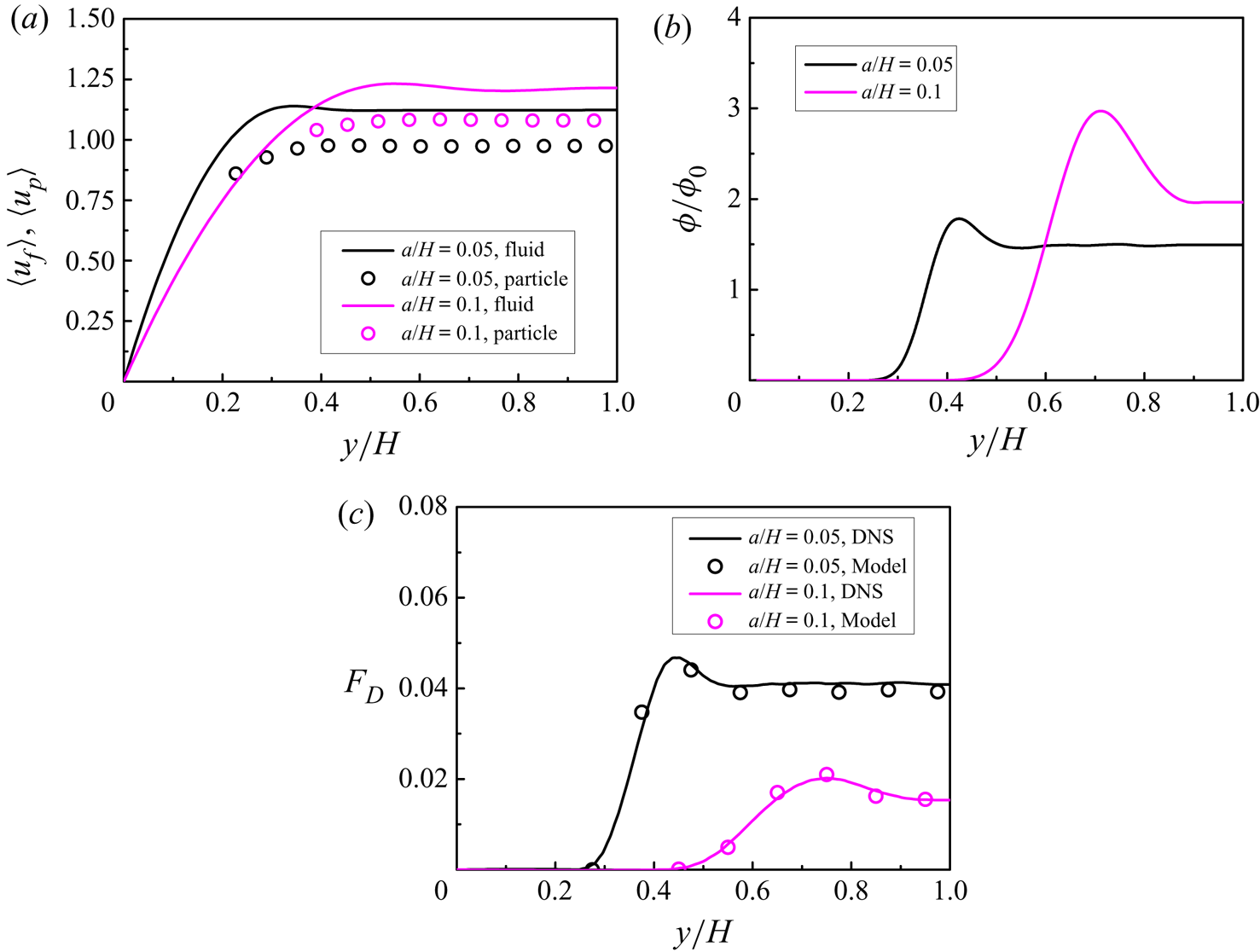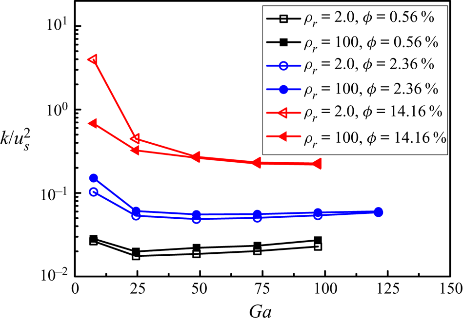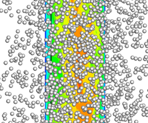

1. Introduction
Particle-laden turbulent flows are ubiquitous in natural and industrial settings, such as fluidized bed, pneumatic transport, fuel combustion and sand storm. Developing accurate models for multiphase turbulent flows is of great importance to better designs of relevant industrial devices. The two-fluid model (i.e. the Euler–Euler method) (Anderson & Jackson Reference Anderson and Jackson1967; Ding & Gidaspow Reference Ding and Gidaspow1990) and the discrete particle (or element) model (i.e. the Euler–Lagrange method) (Tsuji, Kawaguchi & Tanaka Reference Tsuji, Kawaguchi and Tanaka1993; Deen et al. Reference Deen, Van Sint Annaland, Van der Hoef and Kuipers2007; Zhu et al. Reference Zhu, Zhou, Yang and Yu2007) are two models used widely for multiphase flows in engineering applications. The drag model is most important for the accuracy of these two models and is the subject of extensive studies (Tenneti & Subramaniam Reference Tenneti and Subramaniam2014; Wang Reference Wang2020).
In the early years, several empirical drag functions were obtained based on analysis of experimental data (Ergun Reference Ergun1952; Gidaspow Reference Gidaspow1994; Wen & Yu Reference Wen and Yu1966; Zhang & Reese Reference Zhang and Reese2003). A drag correlation proposed by Wen & Yu (Reference Wen and Yu1966) (the Wen–Yu model) from the data of particle sedimentation accounted for the effects of the solid volume fraction at relatively small particle concentrations. Many drag models in the literature (Di Felice Reference Di Felice1994; Mazzei & Lettieri Reference Mazzei and Lettieri2007) were developed from modification of the Wen–Yu model. Recently, Goossens (Reference Goossens2019) presented a review of the empirical drag correlations for a wide range of Reynolds numbers.
In the past two decades, interface-resolved (or particle-resolved) direct numerical simulations (IR-DNS or PR-DNS) have been employed extensively to investigate the mechanisms in fluid–particle interactions and the development of the multiphase flow model, particularly the drag model (van der Hoef et al. Reference van der Hoef, van Sint Annaland, Deen and Kuipers2008; Balachandar & Eaton Reference Balachandar and Eaton2010; Tenneti & Subramaniam Reference Tenneti and Subramaniam2014; Maxey Reference Maxey2017). From interface-resolved simulations of the flow past static arrays of particles at Reynolds numbers up to several hundreds, numerous drag models have been developed (Hill, Koch & Ladd Reference Hill, Koch and Ladd2001; Kandhai, Derksen & Van den Akker Reference Kandhai, Derksen and Van den Akker2003; van der Hoef, Beetstra & Kuipers Reference van der Hoef, Beetstra and Kuipers2005; Beetstra, van der Hoef & Kuipers Reference Beetstra, van der Hoef and Kuipers2007; Holloway, Yin & Sundaresan Reference Holloway, Yin and Sundaresan2010; Tenneti, Garg & Subramaniam Reference Tenneti, Garg and Subramaniam2011; Zaidi, Tsuji & Tanaka Reference Zaidi, Tsuji and Tanaka2014; Bogner, Mohanty & Rüde Reference Bogner, Mohanty and Rüde2015; Tang et al. Reference Tang, Peters, Kuipers, Kriebitzsch and van der Hoef2015; Zhou & Fan Reference Zhou and Fan2015a,Reference Zhou and Fanb; Kravets et al. Reference Kravets, Rosemann, Reinecke and Kruggel-Emden2019). Based on this configuration (spheres with fixed positions and fluctuating velocities), the effects of particle velocity fluctuations on the drag force have been investigated (Huang et al. Reference Huang, Wang, Zhou and Li2017; Balachandar Reference Balachandar2020).
The effects of particle motion on the drag force were investigated with interface-resolved numerical simulations (Luo et al. Reference Luo, Tan, Wang and Fan2016; Rubinstein, Derksen & Sundaresan Reference Rubinstein, Derksen and Sundaresan2016; Tang, Peters & Kuipers Reference Tang, Peters and Kuipers2016; Rubinstein et al. Reference Rubinstein, Ozel, Yin, Derksen and Sundaresan2017; Zaidi Reference Zaidi2018; Tavanashad et al. Reference Tavanashad, Passalacqua, Fox and Subramaniam2019; Tavanashad, Passalacqua & Subramaniam Reference Tavanashad, Passalacqua and Subramaniam2021). The drag models for moving particles were obtained by modifying the above drag correlations based on the static particle packing. Rubinstein et al. (Reference Rubinstein, Derksen and Sundaresan2016, Reference Rubinstein, Ozel, Yin, Derksen and Sundaresan2017) studied the effects of particle motion at the low and high Stokes number limits at low particle Reynolds numbers, and the particle Stokes number was taken into account in the drag correlation. Tang et al. (Reference Tang, Peters and Kuipers2016) observed that the drag force in the dynamic particulate system was significantly greater than that in the static system, and the drag force increased linearly with increasing granular temperature. They proposed a new drag correlation by considering the granular temperature. The interface-resolved simulations of a fluidized bed by Luo et al. (Reference Luo, Tan, Wang and Fan2016) showed that the particle mobility increased the drag force significantly. Zaidi (Reference Zaidi2018) studied the effects of particle inertia on the drag force by simulating numerically the sedimentation of particles, and observed that the drag force decreased with increasing density ratio for particle Reynolds numbers smaller than 200. Zaidi (Reference Zaidi2018) showed that the effects of particle inertia (or density ratio) on the mean drag of settling particles were reflected in either the formation of particle microstructures or particle velocity fluctuations, and proposed a drag correlation incorporating the particle–fluid density ratio. Tavanashad et al. (Reference Tavanashad, Passalacqua, Fox and Subramaniam2019, Reference Tavanashad, Passalacqua and Subramaniam2021) investigated the effects of the density ratio on the drag force by simulating numerically freely evolving particle suspensions in a periodic domain under imposed gradient gradients, and observed that for the homogeneous system, the drag did not change significantly with density ratio even though particle and fluid velocity fluctuations increased with decreasing density ratio.
As for particle sedimentation in a turbulent environment, it was observed that the mean settling speed was increased, compared to that in a quiescent fluid, for particles smaller than the Kolmogorov length scale, due mainly to preferential sweeping of particles on the downward side of eddies (Wang & Maxey Reference Wang and Maxey1993; Yang & Lei Reference Yang and Lei1998; Bec, Homann & Ray Reference Bec, Homann and Ray2014; Gustavsson, Vajedi & Mehlig Reference Gustavsson, Vajedi and Mehlig2014; Rosa et al. Reference Rosa, Parishani, Ayala and Wang2016; Huck et al. Reference Huck, Bateson, Volk, Cartellier, Bourgoin and Aliseda2018). Good et al. (Reference Good, Ireland, Bewley, Bodenschatz, Collins and Warhaft2014) demonstrated that the reduced settling speeds of large particles in their experiments were due to nonlinear drag effects. Chouippe & Uhlmann (Reference Chouippe and Uhlmann2015), Fornari, Picano & Brandt (Reference Fornari, Picano and Brandt2016a) and Fornari et al. (Reference Fornari, Picano, Sardina and Brandt2016b, Reference Fornari, Zade, Brandt and Picano2019) investigated numerically the effects of isotropic turbulence on the settling velocity of particles with the size being the order of or larger than the Kolmogorov scale, and observed that the settling speed of particles was reduced in a turbulent environment.
There have been some works on the effects of turbulence on the drag coefficient of a fixed sphere. The numerical results of Bagchi & Balachandar (Reference Bagchi and Balachandar2003) indicated that the free-stream turbulence had little effect on the time-averaged drag coefficient for relative turbulence intensity between 0.1 and 0.25. Crowe et al. (Reference Crowe, Schwarzkopf, Sommerfeld and Tsuji2011) summarized the previous numerical and experimental works on the effects of turbulence on the drag coefficient, and suggested the use of a standard drag curve for particles in subcritical turbulent flow due to considerable discrepancy in the data for drag coefficient dependence on turbulence. From a model with the assumption of the turbulence fluctuation satisfying a Gaussian distribution and the numerical simulations with the relative turbulence intensity being up to 0.6, Homann, Bec & Grauer (Reference Homann, Bec and Grauer2013) concluded that the relative increase in the drag was proportional to  $C(Re_p)\,I^2$, where
 $C(Re_p)$ is a function of the particle Reynolds number, and
 $I=u'/u_s$ is the relative turbulence intensity.
The drag model for inhomogeneous systems has also been investigated. The filtered method (Igci et al. Reference Igci, Andrews, Sundaresan, Pannala and O'Brien2008) and the heterogeneity-based method (including the energy minimization multi-scale model, i.e. EMMS model) (Li Reference Li1994; Li & Huang Reference Li and Huang2018) are two typical methods accounting for the effects of the mesoscale structure in the coarse computational cell on the drag force (Wang Reference Wang2020). Some models considered the effect of the particle concentration gradient on the drag force (Zhou et al. Reference Zhou, Xiong, Wang, Wang, Ren and Ge2014; Li et al. Reference Li, Wang, Rogers, Zhou and Ge2017; Liu, Ge & Wang Reference Liu, Ge and Wang2020). Ma et al. (Reference Ma, Yu, Chen and Zhou2020) investigated the effects of anisotropic microstructures quantified by a second-order structure tensor on the drag in low-Reynolds-number monodisperse gas–solid suspensions. Wang, Liu & You (Reference Wang, Liu and You2011) proposed a drag model by introducing a non-uniformity coefficient. Rubinstein et al. (Reference Rubinstein, Ozel, Yin, Derksen and Sundaresan2017) concluded that the fluctuation in the solid volume fraction should be included to consider the effect of heterogeneity. By using interface-resolved simulations, a scale-dependent drag model was proposed to account for the heterogeneous structures and particle fluctuating velocity (Liu et al. Reference Liu, Ge and Wang2020). Tavanashad et al. (Reference Tavanashad, Passalacqua and Subramaniam2021) investigated the effects of both particle velocity fluctuations and particle clustering on the drag, by simulating freely evolving suspensions for a wide range of density ratio. Wang (Reference Wang2020) presented a nice review on both homogeneous and heterogeneous drag correlations for dense gas–solid flows.
In the present study, we aim to develop a new drag model for a homogeneous system in which large-scale particle clusters do not exist but the effects of both particle inertia (density ratio) and turbulence may exist, from the interface-resolved simulations of particle sedimentation in a periodic domain and an upward turbulent channel flow. We first obtain the drag model from the modification of the Wen–Yu model, based on our DNS data of particle sedimentation at different Reynolds numbers, volume fractions and density ratios. Although it was shown in the previous studies that at a larger particle–fluid density ratio, the particle fluctuating velocity is lower and the drag is generally smaller (Zaidi Reference Zaidi2018; Tavanashad et al. Reference Tavanashad, Passalacqua, Fox and Subramaniam2019, Reference Tavanashad, Passalacqua and Subramaniam2021), there is a quantitative discrepancy in the effect of the density ratio: it is more significant in the simulations of Zaidi (Reference Zaidi2018) than in the simulations of Tavanashad et al. (Reference Tavanashad, Passalacqua, Fox and Subramaniam2019, Reference Tavanashad, Passalacqua and Subramaniam2021). Thus we focus on the effect of the density ratio, which only very few drag correlations have considered (Wang Reference Wang2020). Then the drag model is modified by considering the effect of turbulence, based on our previous DNS data of upward particle-laden turbulent channel flows (Yu et al. Reference Yu, Xia, Guo and Lin2021). To the best of our knowledge, this is the first work to employ IR-DNS data of the wall-bounded particle-laden turbulent flows to develop a drag correlation incorporating the turbulence effect.
The rest of the paper is organized as follows. In § 2, we present the numerical method and validate its accuracy for the drag force. In § 3, we report the main results on the sedimentation of spherical particles in a periodic box. Then, in § 4, we develop the drag model from the DNS data of vertical turbulent channel flows; the effects of the background turbulence on the drag and the drift velocity are modelled. Finally, we summarize the main contributions of the present study in § 5.
2. Numerical model and validation
2.1. Direct-forcing/fictitious domain method
In the present study, the simulations are conducted with the direct-forcing/fictitious domain (DF/FD) method (Yu & Shao Reference Yu and Shao2007; Yu et al. Reference Yu, Lin, Shao and Wang2016). The key idea of this approach is to fill the interior domain of particles with fictitious fluids, and distribute a pseudo-body force (i.e. distributed Lagrange multiplier) over the solid region to enforce the rigid-body constraints (Glowinski et al. Reference Glowinski, Pan, Hesla and Joseph1999). For simplicity of description, we consider only one particle in the following formulae. Suppose that the particle density, volume, moment of inertia, translational velocity and angular velocity are  $\rho _s$,
 $V_p$,
 $\boldsymbol {J}$,
 $\boldsymbol {U}$ and
 $\boldsymbol {\omega }_p$, respectively. The viscosity and density of the fluid are
 $\mu$ and
 $\rho _f$, respectively. Let
 $P(t)$ represent the solid domain, and
 $\varOmega$ the entire computational domain containing both solid and fluid regions. We introduce the following characteristic scales for the non-dimensionalization:
 $L_c$ for length,
 $U_c$ for velocity,
 $L_c/U_c$ for time,
 ${\rho _f}U_c^2$ for pressure, and
 ${\rho _f}U_c^2/L_c$ for the body force. Then the dimensionless FD formulation for the incompressible fluid can be written as
 $$\begin{gather} \frac{\partial {\boldsymbol{u}}}{\partial t}+{\boldsymbol{u}} \boldsymbol{\cdot} \boldsymbol{\nabla} {\boldsymbol{u}}= \frac{\nabla ^2 {\boldsymbol{u}}}{Re}-\boldsymbol{\nabla} p +{\boldsymbol{\lambda}} \quad {\rm in} \ {\varOmega}, \end{gather}$$
 $$\begin{gather}{\boldsymbol{u}}={\boldsymbol{U}}+{\boldsymbol{\omega}_p} \times {\boldsymbol{r}}\quad {\rm in} \ {P(t)}, \end{gather}$$
 $$\begin{gather}\boldsymbol{\nabla} \boldsymbol{\cdot} {\boldsymbol{u}} =0 \quad {\rm in}\ {\varOmega}, \end{gather}$$
 $$\begin{gather}(\rho_r -1)V_p^*\left(\frac{{\rm d} {\boldsymbol{U}}}{{\rm d} t}-Fr\, \frac{\boldsymbol{g}}{ g}\right)={-}\int_P {\boldsymbol{\lambda}} \,{\rm d}\kern0.06em {\boldsymbol{x}}, \end{gather}$$
 $$\begin{gather}(\rho_r -1)\,\frac{{\rm d} ({\boldsymbol{J}}^* \boldsymbol{\cdot}{\boldsymbol{\omega }}_p)}{{\rm d} t}={-}\int_P{\boldsymbol{r}}\times{\boldsymbol{\lambda}}\,{\rm d}\kern0.06em {\boldsymbol{x}}, \end{gather}$$
where  $\boldsymbol {u}$,
 $p$,
 $\boldsymbol {\lambda }$ and
 $\boldsymbol {r}$ represent the fluid velocity, pressure, pseudo-body force and position vector with respect to the mass centre of the particle, respectively. Also,
 $\rho _r=\rho _s/\rho _f$ is the particle to fluid density ratio,
 $Re$ is the Reynolds number defined by
 $Re = {\rho _f}{U_c}L_c/\mu$, and
 $Fr$ is the Froude number defined by
 $Fr = gL_c/U_c^2$, with
 $\boldsymbol {g}$ being the gravitational acceleration,
 $V_p^*$ the dimensionless particle volume define by
 $V_p^* = {V_p}/L_c^3$, and
 ${{\boldsymbol {J}}^*}$ the dimensionless moment of inertia defined by
 ${{\boldsymbol {J}}^*} = {{\boldsymbol {J}}^*}/{\rho _s}L_c^5$.
A fractional-step temporal scheme is used to decouple the system (2.1)–(2.5) into two subproblems.
(1) Fluid subproblem for  ${\boldsymbol {u}}^*$ and
 $p$:
 $$\begin{gather} \frac{{\boldsymbol{u}}^*-{\boldsymbol{u}}^n}{\Delta t}-\frac{1}{2}\,\frac{\nabla ^2{\boldsymbol{u}}^*}{Re}={-}\boldsymbol{\nabla} p-\frac{1}{2}\,[3({\boldsymbol{u}} \boldsymbol{\cdot}\boldsymbol{\nabla} {\boldsymbol{u}})^n-({\boldsymbol{u}} \boldsymbol{\cdot}\boldsymbol{\nabla} {\boldsymbol{u}})^{n+1}]+\frac{1}{2}\,\frac{\nabla^2{\boldsymbol{u}}^n}{Re}+{\boldsymbol{\lambda}}^n, \end{gather}$$
 $$\begin{gather}\boldsymbol{\nabla}\boldsymbol{\cdot}{\boldsymbol{u}}^*=0. \end{gather}$$
An efficient finite-difference projection method on a homogeneous half-staggered grid is used. All spatial derivatives are discretized with a second-order central difference scheme.
(2) Particle subproblem for  ${\boldsymbol {U}}^{n+1}$,
 ${\boldsymbol {\omega }}_p^{n+1}$,
 ${\boldsymbol {\lambda }}^{n+1}$ and
 ${\boldsymbol {u}}^{n+1}$:
 $$\begin{gather} \rho_r V_p^*\,\frac{{\boldsymbol{U}}^{n+1}}{\Delta t}=(\rho_r-1) V_p^* \left(\frac {{\boldsymbol{U}}^n}{\Delta t}-Fr\,\frac{\boldsymbol{g}}{g}\right)+\int_P \left({\frac{{\boldsymbol{u}}^*}{\Delta t}- {\boldsymbol{\lambda}}^n}\right){\rm d}\kern0.06em {\boldsymbol{x}}, \end{gather}$$
 $$\begin{gather}\rho_r\,\frac{{\boldsymbol{J}}^{*}\boldsymbol{\cdot} {\boldsymbol{\omega} }_p^{n+1}}{\Delta t}=(\rho_r-1) \left[\frac{{\boldsymbol{J}}^{*} \boldsymbol{\cdot} {\boldsymbol{\omega} }_p^{n}}{\Delta t}-{\boldsymbol{\omega} }_p^{n} \times ({\boldsymbol{J}}^{*} \boldsymbol{\cdot} {\boldsymbol{\omega} }_p^{n})\right]+\int_P {\boldsymbol{r}} \times \left({\frac{{\boldsymbol{u}}^*}{\Delta t}- {\boldsymbol{\lambda}}^n}\right) {\rm d}\kern0.06em {\boldsymbol{x}}. \end{gather}$$
Then the pseudo-body force  $\boldsymbol {\lambda }$ defined at the Lagrangian nodes is updated from
 \begin{equation} {\boldsymbol{\lambda}}^{n+1}=\frac{{\boldsymbol{U}}^{n+1}+{\boldsymbol{\omega}}_p^{n+1}\times {\boldsymbol{r}}-{\boldsymbol{u}}^*}{\Delta t}+{\boldsymbol{\lambda}}^n. \end{equation}
Finally, the fluid velocities  ${\boldsymbol {u}}^{n+1}$ at the Eulerian nodes are corrected as
 \begin{equation} {\boldsymbol{u}}^{n+1}={\boldsymbol{u}}^{*}+\Delta t\, ({\boldsymbol{\lambda}}^{n+1}-{\boldsymbol{\lambda}}^{n}). \end{equation}
In the above manipulations, a discrete  $\delta$ function in the form of a trilinear function is used to transfer quantities between the Eulerian and Lagrangian nodes.
2.2. Collision strategy
In order to handle the unresolved short-range hydrodynamic interactions and the collision between particles, a discrete element method (DEM) with the lubrication correction is used (Xia et al. Reference Xia, Xiong, Yu and Zhu2020a). In our DEM model, the contact forces acting on particle  $i$ by particle
 $j$ are given as (Crowe et al. Reference Crowe, Schwarzkopf, Sommerfeld and Tsuji2011)
 $$\begin{gather} {{\boldsymbol{F}}_{ij,n}} = ({-{k_n}\delta_n^{3/2} - {\eta _n}{\boldsymbol{u}_{ij}\boldsymbol{\cdot} \boldsymbol{n}}})\boldsymbol{n} , \end{gather}$$
 $$\begin{gather}{{\boldsymbol{F}}_{ij,t}} = (- {k_t}{{\delta}_t} - {\eta _t}{\boldsymbol{u}_{ij} \boldsymbol{\cdot} \boldsymbol{t}})\boldsymbol{t}, \end{gather}$$
where  ${{\boldsymbol {F}}_{ij,n}}$,
 $\delta _n$,
 $k_n$ and
 $\eta _n$ are the normal contact force, overlap, stiffness constant and damping coefficient, respectively, and
 ${{\boldsymbol {F}}_{ij,t}}$,
 $\delta _t$,
 $k_t$ and
 $\eta _t$ are the corresponding parameters in the tangential direction. Also,
 $\boldsymbol {n}$ is the normal vector pointing from the centre of particle
 $i$ to that of particle
 $j$, and
 $\boldsymbol {t}$ is the unit tangential vector. If
 $\boldsymbol {u}_{ij}=\boldsymbol {u}_{i}-\boldsymbol {u}_{j}$ denotes the relative velocity between particles, then the relative normal velocity can be written as
 $\boldsymbol {u}_{ij,n} = (\boldsymbol {u}_{ij} \boldsymbol {\cdot } \boldsymbol {n})\boldsymbol {n}$, and the slip velocity at the contact point is
 \begin{equation} \boldsymbol{u}_{ij,t} = \boldsymbol{u}_{ij}-\boldsymbol{u}_{ij,n}+(a_i \boldsymbol{\omega}_i \times \boldsymbol{n}+a_j \boldsymbol{\omega}_j \times \boldsymbol{n}), \end{equation}
where  $a$ denotes the radius of the particle, and
 $\boldsymbol {\omega }$ is the rotational velocity of the particle.
The values of  $k_n$ and
 $k_t$ are given by Hertzian contact theory and Mindlin's theory (Crowe et al. Reference Crowe, Schwarzkopf, Sommerfeld and Tsuji2011) as
 $$\begin{gather} {k_n}=\frac{4}{3}{\left( {\frac{{1 - \sigma _i^2}}{{{E_i}}} + \frac{{1 - \sigma _j^2}}{{{E_j}}}} \right)^{ - 1}}{\left( {\frac{{{a_i} + {a_j}}}{{{a_i}{a_j}}}} \right)^{ - {1/2}}}, \end{gather}$$
 $$\begin{gather}k_{t}=8\left(\frac{2-\sigma_{i}}{G_{i}}+\frac{2-\sigma_{j}}{G_{j}}\right)^{{-}1}\left(\frac{a_{i}+a_{j}}{a_{i} a_{j}}\right)^{{-}1/2}\delta_{n}^{1/2}, \end{gather}$$
where  $E$ and
 $\sigma$ are the Young's modulus and Poisson ratio, respectively, and
 $G = E /2(1 + \sigma )$ is the particle shear modulus. Damping coefficients
 $\eta _n$ and
 $\eta _t$ are given as
 \begin{equation} \eta _n = {\alpha_n}\sqrt {{m_p}{k_n}}\,\delta _n^{{1 / 4}},\quad \eta_t = {\alpha_t}\sqrt {{m_p}{k_t}}\,\delta _t^{{1 /4}}, \end{equation}
where  ${m_p} = {{{m_i}{m_j}} /( {{m_i} + {m_j}} )}$, and
 $\alpha _n$ is a constant related to the dry coefficient of restitution
 $e_d$ (Tsuji, Tanaka & Ishida Reference Tsuji, Tanaka and Ishida1992).
If  $| {{\boldsymbol {F}_t}} | \geqslant \mu _c\,| {{\boldsymbol {F}_n}} |$, then the tangential force is given by the Coulomb-type friction law
 \begin{equation} {\boldsymbol{F}}_{t}={-}\mu_c\,|{\boldsymbol{F}}_{n}|\,{\boldsymbol{t}}, \end{equation}
where  $\mu _c$ is the friction coefficient. In the present simulations, we set
 $e_d=0.97$,
 $\sigma = 0.33$,
 $\mu _c = 0.3$ for the particle–particle collision, and
 $\mu _c = 0.2$ for the particle–wall collision, unless otherwise stated. The time step for the collision
 $\Delta t_c$ is set to be one-tenth of that for the flow solution
 $\Delta t$.
Since the fictitious domain method is based on a fixed Cartesian grid, the correction of the lubrication force is needed when two particles are very close to each other. The lubrication correction has the form
 \begin{equation} \boldsymbol{F}_{lub}={-}6 {\rm \pi}\mu a \boldsymbol{u}_n\left[\lambda(\epsilon)-\lambda\left(\epsilon_{al}\right)\right], \end{equation}
where  $\boldsymbol {u}_n$ is the normal relative velocity between two equal spherical particles or between a spherical particle and a planar surface, and
 $\epsilon _{al}=\Delta x/a$ is the threshold gap below which the lubrication correction is activated, where
 $a$ represents the radius of particle and
 $\Delta x$ is the grid size. Also,
 $\lambda (\epsilon )$ is a function of the normalized gap distance
 $\epsilon = \zeta _n/a$ (Jeffrey Reference Jeffrey1982), so
 $$\begin{gather} \lambda (\epsilon) = \frac{1}{{4\epsilon }} - \frac{9}{{40}}\ln (\epsilon) - \frac{3}{{112}}\,\epsilon \ln (\epsilon) + 0.673, \end{gather}$$
 $$\begin{gather}\lambda (\epsilon) = \frac{1}{\epsilon } - \frac{1}{5}\ln (\epsilon) - \frac{1}{{21}}\,\epsilon \ln (\epsilon) + 0.9713. \end{gather}$$
Note that the lubrication correction is kept constant for  $\epsilon < \epsilon _1$ to account for the lubrication force saturation due to the effect of the surface roughness. In addition, the lubrication force correction is turned off for
 $\epsilon \leqslant -\epsilon _2$ when two particles overlap and the squeezing fluid film is damaged. The collision model combined with the lubrication correction for
 $\epsilon _1=0.001$ and
 $\epsilon _2=0.001$ has been validated (Xia et al. Reference Xia, Xiong, Yu and Zhu2020a).
2.3. Validation
The accuracy of our code has been demonstrated in previous studies for turbulent channel flow (Wang et al. Reference Wang, Peng, Guo and Yu2016; Yu et al. Reference Yu, Lin, Shao and Wang2016, Reference Yu, Zhu, Wang and Shao2019) and particle sedimentation (Yu & Shao Reference Yu and Shao2007; Shao, Wu & Yu Reference Shao, Wu and Yu2012). Here, we validate further our code via three problems: (a) sedimentation of a single sphere in a periodic box; (b) rising of a single sphere in an inclined channel; (c) flow past a fixed bed of randomly distributed spheres.
2.3.1. Sedimentation of a sphere in a periodic box
The DF/FD simulation of the sedimentation of a single sphere in a pipe with grid resolution  $d_p/\Delta x=12.8$ (here,
 $d_p$ is the particle diameter, and
 $\Delta x$ is the mesh size) was shown to have good accuracy for particle Reynolds numbers below 100 (Yu & Shao Reference Yu and Shao2007). Here, we intend to examine whether our code can predict accurately the particle settling velocity in a periodic domain for particle Reynolds numbers below 300. The computational domain is a periodic box of size
 $L_x=80d_p$,
 $L_y=L_z=20d_p$. The gravity points to the negative
 $x$-direction. Three grid resolutions
 $d_p/\Delta x=\{6.4, 12.8, 25.6\}$ are used to examine the mesh convergence of the results. The terminal settling Reynolds number
 $Re_T$ is computed using the terminal settling velocity of the sphere
 $u_T$. The drag coefficient is computed from
 \begin{equation} C_d=\frac{8 (\rho_s-\rho_f)gV_p}{{\rm \pi} d_p^2 \rho_{f} u_T^{2}}. \end{equation}
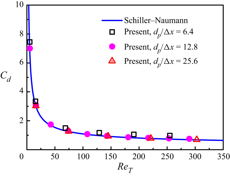
Figure 1 compares the computed drag coefficients and the standard drag coefficient of Schiller & Naumann (Reference Schiller and Naumann1933):
 \begin{equation} C^{SN}_{d}=\frac{24}{Re_{T}}\left(1+0.15\,Re_{T}^{0.687}\right). \end{equation}
It is observed that the results from  $d_p/\Delta x=12.8$ and 25.6 are in good agreement with the standard drag coefficient. Our code with
 $d_p/\Delta x=12.8$ slightly overpredicts the drag, with maximum relative error about 3 % at high particle Reynolds numbers. Due to the limited computational resources, we choose
 $d_p/\Delta x=12.8$ for the present simulations, and the highest particle Reynolds number for the drag correlation in our simulations is around 132.
Computed drag coefficients  $C_d$ for a sphere settling in a periodic domain at different grid resolutions, as compared to the standard drag coefficient.

2.3.2. Rising of a sphere in an inclined channel
The rising of a light sphere in an inclined channel is simulated with our DF/FD method. Lomholt et al. (Reference Lomholt, Stenum and Maxey2002) reported the experimental and numerical results on this test problem. The channel is tilted angle  $\theta = 8.23^{\circ }$ with the vertical direction. The particle diameter is
 $d_p=2\ {\rm mm}$, the fluid density is
 $\rho _f = 1.115\ {\rm g}\ {\rm cm}^{-3}$, the particle density is
 $\rho _s = 1.081\ {\rm g}\ {\rm cm}^{-3}$, and the fluid kinematic viscosity is
 $\nu = 3.125\ {\rm mm}^2\ {\rm s}^{-1}$. These parameter values yield
 $Re_p^{{{Stokes }}} = 13.6$, which is the Reynolds number based on the Stokes settling velocity
 $W = {{{d_p^2}}}/{{18\mu }}\,| {{\rho _s} - {\rho _f}} |\,g$ and defined as
 \begin{equation} Re_p^{{{Stokes}}} = \frac{{{d_p}W}}{\nu } = \frac{{d_p^3}}{{18\nu }}\left| {{\rho _r} - 1} \right|g. \end{equation}
The Galileo number is defined as
 \begin{equation} Ga = \frac{{\sqrt {d_p^3\left( {{\rho _r} - 1} \right)g} }}{\nu }, \end{equation}
and  $Ga = \sqrt {18\,Re_p^{{{Stokes }}}}=15.65$.
The channel size in the experiments is  $150\ {\rm mm} \times 10\ {\rm mm} \times 100 {\rm mm}$. As in the simulations of Lomholt et al. (Reference Lomholt, Stenum and Maxey2002), we take the channel width as only 10 mm, and reduce the channel height and depth to save the computational cost. In our simulations, the computational domain size is
 $80\ {\rm mm} \times 10\ {\rm mm} \times 40\ {\rm mm}$ in the
 $x$ (upward),
 $y$ (lateral) and
 $z$ (spanwise) directions, respectively. The periodic boundary condition is imposed in the
 $x$- and
 $z$-directions, and the no-slip velocity boundary condition is imposed on the walls in the
 $y$-direction. We denote the channel half-width as
 $H$. Thus
 $d_p=0.4H$. The mesh resolution is
 $d_p/\Delta x=12.8$.
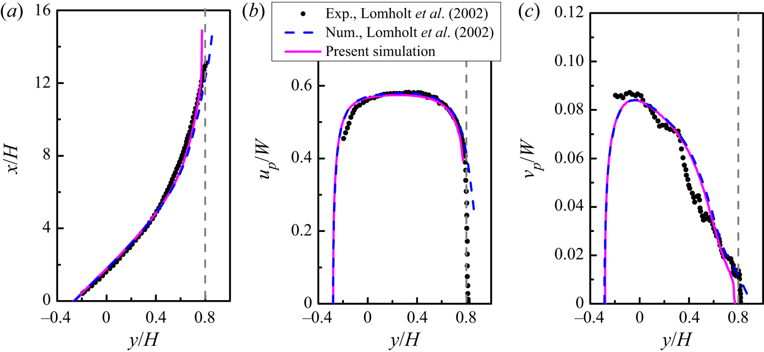
Figure 2 compares the results from our simulation and the experimental and numerical results of Lomholt et al. (Reference Lomholt, Stenum and Maxey2002) for  $Re_p^{{{Stokes }}} = 13.6$. The numerical results of Lomholt et al. (Reference Lomholt, Stenum and Maxey2002) were obtained using the force coupling method. Our results are in remarkably good agreement with the numerical results of Lomholt et al. (Reference Lomholt, Stenum and Maxey2002), except for the wall region where the particle of Lomholt et al. (Reference Lomholt, Stenum and Maxey2002) penetrated the wall because no collision model was used by them. Both numerical results agree well with the experiments.
Comparison of the present simulation and the previous experimental and numerical results (Lomholt, Stenum & Maxey Reference Lomholt, Stenum and Maxey2002) for a sphere rising in an inclined channel at  $Re_p^{Stokes} = 13.6$: (a) sphere trajectory, (b) velocity in the upward direction, and (c) velocity in the lateral direction. The position is normalized with the channel half-width, and the velocity is normalized with the Stokes settling velocity. The vertical dashed line denotes the position where the particle touches the wall.

2.3.3. Flow past a fixed bed of randomly distributed spheres
Due to the lack of numerical benchmarks for the multi-particle settling system suitable for direct quantitative comparison, we provide a comparison of present results on the drag of fixed-bed simulations with some existing drag models established from DNS (Beetstra et al. Reference Beetstra, van der Hoef and Kuipers2007; Tenneti et al. Reference Tenneti, Garg and Subramaniam2011; Zaidi et al. Reference Zaidi, Tsuji and Tanaka2014; Bogner et al. Reference Bogner, Mohanty and Rüde2015; Tang et al. Reference Tang, Peters, Kuipers, Kriebitzsch and van der Hoef2015).
Following these studies, a constant flow rate is applied for the flow past a fixed array of  $N_p$ randomly distributed spheres in a cubic box of edge length
 $L$, and the flow is assumed triply periodic in space. A summary of parameter settings is given in table 1. The Reynolds number
 $Re_m$ is defined as
 \begin{equation} Re_m=\frac{\rho_f (1-\phi) u_{m} d_p}{\mu}, \end{equation}
where  $u_m$ is the fluid average velocity, and
 $\phi$ is the particle volume fraction. The average drag on one sphere is defined as
 \begin{equation} \langle F_{d}\rangle=\frac{1}{N_{p}} \sum_{i=1}^{N_{p}} F_i, \end{equation}
where  $F_i$ is the hydrodynamic force on the
 $i$th sphere. The Stokes drag acting on an isolated sphere,
 $F_{Stokes}=3 {\rm \pi}\mu d_p (1-\phi ) u_{m}$, is employed to normalize the average drag
 $\langle F_{d}\rangle$. We compute the dimensionless drag
 $F(Re_m, \phi )=\langle F_{d}\rangle /F_{Stokes}$ for
 $2 \leqslant Re_m \leqslant 150$ at
 $\phi =0.1$. The present results for two grid resolutions (
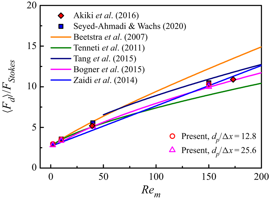
 $d_p/\Delta x=12.8$ and 25.6) are presented in figure 3 for comparison.
Summary of the simulation settings used for IR-DNS of fixed beds of spheres. Here,  $\phi =N_p {\rm \pi}d_p^3/(6L^3)$ is the solid volume fraction.

Comparison of the present drags with the previous drag correlations (Beetstra et al. Reference Beetstra, van der Hoef and Kuipers2007; Tenneti et al. Reference Tenneti, Garg and Subramaniam2011; Zaidi et al. Reference Zaidi, Tsuji and Tanaka2014; Bogner et al. Reference Bogner, Mohanty and Rüde2015; Tang et al. Reference Tang, Peters, Kuipers, Kriebitzsch and van der Hoef2015) and the previous IR-DNS results (Akiki et al. Reference Akiki, Jackson and Balachandar2016; Seyed-Ahmadi & Wachs Reference Seyed-Ahmadi and Wachs2020). Each data point of our work is obtained with five different realizations.

It is observed in figure 3 that there are significant discrepancies among different drag correlations. The reasons for a discrepancy may include the differences in numerical algorithms, spatial resolutions and computation domain sizes, and in particular we note that some correlations are obtained for a wide range of parameters (e.g. including the regime of much higher particle volume fractions and particle Reynolds numbers than the regime studied here), thus the difference for a specific parameter regime can be significant. The differences in the predictions by different empirical drag correlations may reach orders of magnitude (Wang Reference Wang2020). Nevertheless, our data seem to agree well with the drag correlation of Bogner et al. (Reference Bogner, Mohanty and Rüde2015). In addition, the data of Akiki, Jackson & Balachandar (Reference Akiki, Jackson and Balachandar2016) and Seyed-Ahmadi & Wachs (Reference Seyed-Ahmadi and Wachs2020) in figure 3 were obtained directly with IR-DNS, and our results are in good agreement with them. We note that Tenneti et al. (Reference Tenneti, Garg and Subramaniam2011) used higher mesh resolutions than ours for high particle Reynolds numbers in order to resolve the boundary layer around the particle surface.
3. Results on sedimentation of particles in a periodic domain
3.1. Simulation set-up
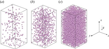
As shown in figure 4, the computational domain is a periodic rectangular box, with size  $40{d_p} \times 20{d_p} \times 20{d_p}$. Our tests for
 $(\phi,Ga,\rho _r) = (14.16\,\%,73,2.0)$ and
 $(2.36\,\%,121,2.0)$ showed that the particle mean settling velocity (or drag coefficient) changes little as the domain size is increased further. The grid resolution is
 $d_p/\Delta x=12.8$. The gravitational acceleration
 $\boldsymbol {g}$ points along the negative
 $x$-direction. Initially, particles are placed randomly in the computational domain, and the volumetric flux of the suspension is kept at zero via a dynamically adjusted pressure gradient.
Sketches of the particle sedimentation in a fully periodic domain for three different particle volume fractions: (a)  $\phi = 0.59\,\%$, (b)
 $\phi = 2.36\,\%$, and (c)
 $\phi = 14.16\,\%$.

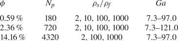
We select four values of the density ratio, ranging from 2 to 1000, and three solid volume fractions, ranging from 0.59 % to 14.16 %. The parameter settings are listed in table 2.
Simulation settings for particles settling in a fully periodic domain, where  $N_p$ is the particle number, and
 $\phi$ is the particle volume fraction.

The apparent slip velocity  $u_s$ is defined as the difference in the average velocity between fluid and solid phases in the gravity direction as
 \begin{equation} u_s=\langle{u_f}\rangle-\langle u_p\rangle. \end{equation}
The notation  $\langle {\cdot } \rangle$ denotes the phase average taken for the fluid or solid domain and time. The particle Reynolds number is defined as
 $Re_p={d_p}\, |u_s|/{\nu }$.
3.2. Drag correlation
The average momentum equations at the steady state for the fluid and solid phases in the direction of gravity for the homogeneous system read, respectively, (Yu et al. Reference Yu, Xia, Guo and Lin2021),
 $$\begin{gather} (1-\phi)\left(-\frac{{\rm d} p_{e}}{{\rm d} x}\right)-F_D=0, \end{gather}$$
 $$\begin{gather}\phi\left(-\frac{{\rm d} p_{e}}{{\rm d}x}\right)-\phi\left(\rho_{s}-\rho_{f}\right)g+F_D=0, \end{gather}$$
where  $F_D = (1/V)\sum _k {F_k}$ is the volume-averaged drag force in which
 $F_k$ denotes the drag force on the
 $k$th particle, and the averaging volume
 $V$ is the entire computational domain. From (3.2) and (3.3), the volume-averaged drag can be computed from
 \begin{equation} F_D=(1-\phi)\left(-\frac{{\rm d} p_{e}}{{\rm d} x}\right)=\phi (1-\phi) (\rho_{s}-\rho_{f}) g. \end{equation}
We compared the mean drag force from (3.4) to that from averaging the forces on all particles, and observed that two results are in excellent agreement with each other (not shown here). We take the following form for the drag correlation:
 \begin{equation} {{F_D} = \beta\,|u_s|}, \end{equation}
where  $\beta$ is the momentum transfer coefficient defined as
 \begin{equation} \beta = \frac{3}{4}\,{C_d}\,\frac{{{\rho _f}\phi (1 - \phi )\,|u_s|}}{{{d_p}}}\,{(1 - \phi )^{ - n}}, \end{equation}
in which  $n$ is the exponent of the correction function for the volume fraction, and
 $C_d$ is the modified drag coefficient for one particle defined as
 \begin{equation} C_d=\frac{24}{(1-\phi)\,R e_{p}}\left(1+0.15\left((1-\phi)\,Re_{p}\right)^{0.687}\right). \end{equation}
The Wen–Yu formula (Wen & Yu Reference Wen and Yu1966) with  $n=2.65$ was proposed from the experimental data of particle sedimentation, and it is used widely for the particle-laden flows for
 $\phi \leqslant 0.2$. It was suggested that the exponent
 $n$ should depend on the particle Reynolds number
 $Re_p$ (Di Felice Reference Di Felice1994; Mazzei & Lettieri Reference Mazzei and Lettieri2007).
The volume-averaged drag forces  $F_D$ obtained from (3.4) at different particle Reynolds numbers
 $Re_p$ for
 $\phi =0.59\,\%$,
 $2.36\,\%$ and 14.16 % are shown in figure 5. Some existing drag correlations (Wen & Yu Reference Wen and Yu1966; Beetstra et al. Reference Beetstra, van der Hoef and Kuipers2007; Mazzei & Lettieri Reference Mazzei and Lettieri2007; Tavanashad et al. Reference Tavanashad, Passalacqua and Subramaniam2021) are also shown for comparison. From figure 5, our drags are always larger than those of Wen & Yu (Reference Wen and Yu1966), smaller than those of (Beetstra et al. Reference Beetstra, van der Hoef and Kuipers2007) at relatively large
 $\phi$ and
 $Re_p$, and most close to those of Tavanashad et al. (Reference Tavanashad, Passalacqua and Subramaniam2021).
Average drag  $F_D$ normalized with
 ${\rho _f}{\nu ^2}/d_p^3$ as a function of the particle Reynolds number
 $Re_p$ for (a)
 $\phi =0.59\,\%$, (b)
 $\phi =2.36\,\%$, and (c)
 $\phi =14.16\,\%$. The existing drag correlations (Wen & Yu Reference Wen and Yu1966; Beetstra et al. Reference Beetstra, van der Hoef and Kuipers2007; Mazzei & Lettieri Reference Mazzei and Lettieri2007; Tavanashad et al. Reference Tavanashad, Passalacqua and Subramaniam2021) are also shown for comparison.

Our results show that the increase in the density ratio  $\rho _r$ enhances the particle Reynolds number (or mean settling velocity) at the same Galileo number, which means that the drag is smaller for more dense particles at the same Reynolds number. However, this effect of the density ratio on the drag is insignificant, as shown in figure 5 and more clearly in figures 8(c,d), being consistent with the observation of Tavanashad et al. (Reference Tavanashad, Passalacqua, Fox and Subramaniam2019, Reference Tavanashad, Passalacqua and Subramaniam2021).
The intensity of the particle velocity fluctuation at the statistically stationary state is quantified by the particle granular temperature  $T$, given by
 \begin{equation} T=\tfrac{1}{3}\left(u_{p}^{\prime 2}+v_{p}^{\prime 2}+w_{p}^{\prime 2}\right), \end{equation}
where  $u'_p$,
 $v'_p$ and
 $w'_p$ are the components of particle velocity fluctuation in three directions, respectively.
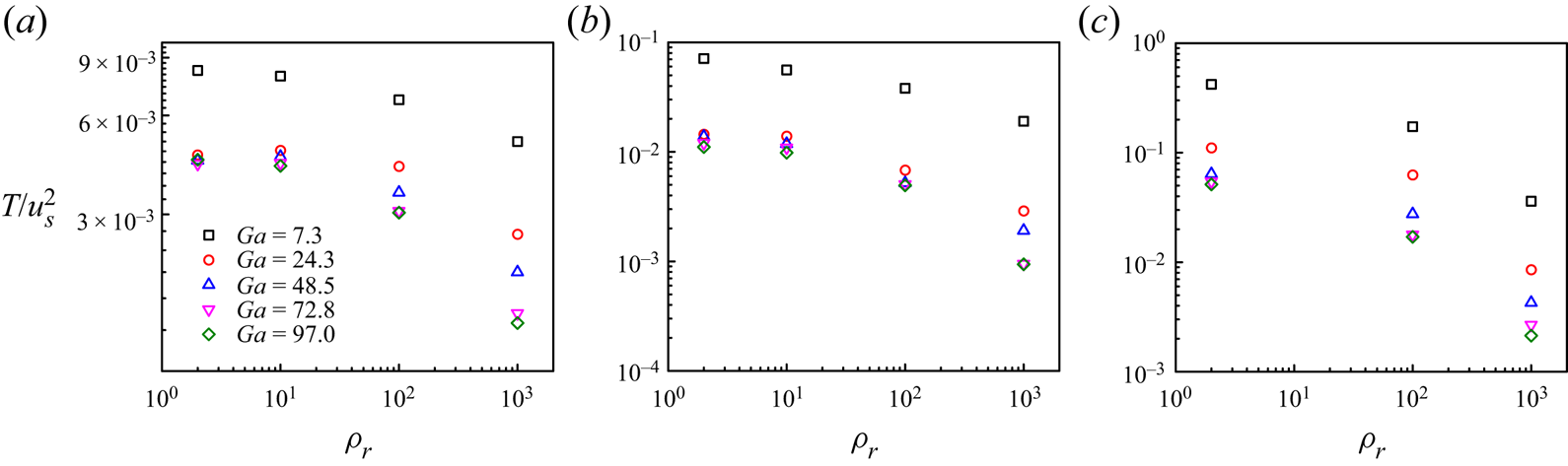
Figure 6 shows the granular temperature normalized with the mean slip velocity squared as a function of density ratio for different volume fractions and Galileo numbers. In general, the value of  $T/u_s^2$ decreases with increasing
 $\rho _r$. The same trend was observed for freely evolving gas–solid flows under imposed pressure gradients (Tang et al. Reference Tang, Peters and Kuipers2016; Tenneti, Mehrabadi & Subramaniam Reference Tenneti, Mehrabadi and Subramaniam2016), which showed a correlation
 $T/u_s^2 \sim \rho _r^{-1}$. Tavanashad et al. (Reference Tavanashad, Passalacqua, Fox and Subramaniam2019) studied the normalized granular temperature
 $T/u_s^2$ for
 $0.001 \leqslant \rho _r \leqslant 1000$ at particle Reynolds number 20, and they reported that
 $T/u_s^2$ was almost unaffected by the density ratio for
 $\rho _r \leqslant 0.1$ due to the added mass effect. The results in figure 6 show a similar insensitivity of
 $T/u_s^2$ to the density ratio at
 $\rho _r \leqslant 10$. On the other hand,
 $T/u_s^2$ decreases with increasing
 $Ga$.
 $T/u_s^2$ is extraordinarily large at
 $Ga=7.3$, compared to the cases for
 $Ga \geqslant 24.3$. In the following, we attempt to provide an explanation for this.
Normalized granular temperature  $T/u_s^2$ as a function of density ratio
 $\rho _r$ for (a)
 $\phi =0.59\,\%$, (b)
 $\phi =2.36\,\%$, and (c)
 $\phi =14.16\,\%$.

The large-scale flow structure of the size comparable to the computational cell was observed in the simulations of particle sedimentation in a periodic box at low  $Re_p$, thus the velocity fluctuations diverged with the size of the computational cell (Ladd Reference Ladd1997). We examine whether such large-scale flow structures exist in our simulations at
 $\rho _r=2.0$ and
 $\phi =2.36\,\%$ for two different domain sizes: (1)
 $40{d_p} \times 20{d_p} \times 20{d_p}$ (denoted as ‘
 $S$’), and (2)
 $80{d_p} \times 40{d_p} \times 40{d_p}$ (denoted as ‘
 $L$’). The two-point spatial correlations of fluid velocity fluctuations in the
 $x$- and
 $z$-directions,
 $R_{uu}$ and
 $R_{ww}$, are computed from
 $$\begin{gather} R_{uu}(\Delta z)=\frac{\langle\overline{u'(x,y,z,t)\,u'(x,y,z+\Delta z,t)}\rangle}{\langle\overline{u'(x,y,z,t)^2}\rangle}, \end{gather}$$
 $$\begin{gather}R_{ww}(\Delta x)=\frac{\langle\overline{w'(x,y,z,t)\,w'(x+\Delta x,y,z,t)}\rangle}{ \langle\overline{w'(x,y,z,t)^2}\rangle}, \end{gather}$$
where the angle bracket  $\langle \cdot \rangle$ represents time averaging, and the overbar denotes spatial averaging, excluding grid points lying in the solid domain.
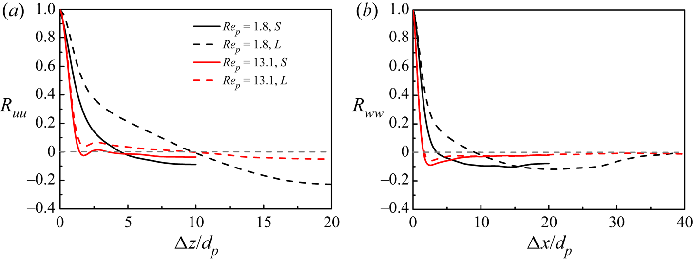
Figures 7(a) and 7(b) show  $R_{uu}$ versus the separation in the
 $z$-direction and
 $R_{ww}$ versus the separation in the
 $x$-direction at
 $Ga=7.3$ and 24.3 for
 $(\rho _r, \phi )=(2.0, 2.36\,\%)$, respectively. The pronounced negative
 $R_{uu}$ and
 $R_{ww}$ at a large separation of the half-width of the computational domain – i.e. 10
 $d_p$ for the smaller box and 20
 $d_p$ for the larger box, at the low Reynolds number
 $Re_p=1.8$ – indicate the existence of a large-scale flow structure with the size of the box width. By contrast, at
 $Re_p=13.1$, a more rapid drop in
 $R_{uu}$ and
 $R_{ww}$ with increasing separation is observed, and both
 $R_{uu}$ and
 $R_{ww}$ are small for separations larger than five particle diameters, which indicates that the large-scale structure becomes quite weak, if it exists.
Two-point autocorrelations of the fluid velocity fluctuations (a)  $R_{uu}$ and (b)
 $R_{ww}$ computed for two different computational domain sizes at
 $Ga=7.3$ and
 $24.3$, and
 $(\rho _r,\phi )=(2.0,2.36\,\%)$.

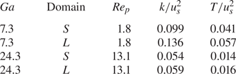
It can be imagined that the large-scale flow structure can lead to a large fluid velocity fluctuation (or pseudo-turbulent kinetic energy), and thereby a large particle velocity fluctuation (or particle granular temperature) due to the entrainment of the particles by the fluid. As shown in table 3, the relative fluid pseudo-turbulent kinetic energy  $k/u_s^2$ and particle granular temperature
 $T/u_s^2$ increase significantly with increasing domain size for the low Reynolds number
 $Re_p=1.8$, due to the presence of the large-scale structure, whereas for
 $Re_p=13.1$, the velocity fluctuation intensity does not change much with the increase in the domain size. Thus the extraordinarily large
 $T/u_s^2$ at
 $Ga=7.3$ in figure 6 is explained.
Comparison of the particle Reynolds number  $Re_p$ relative to particle-induced turbulent kinetic energy
 $(k/u_s^2)$ and particle granular temperature
 $T/u_s^2$ for different domain sizes.

For our dynamic simulations of particle sedimentation, the drag force is prescribed in (3.4), and the slip velocity is computed to determine the drag coefficient. The particle Reynolds number  $Re_p$ is computed from the slip velocity, and the independence of
 $Re_p$ from the box size in table 3 indicates that the interphase drag coefficient does not depend on the box size for
 $Re_p=1.8$ and 13.1. This means that the drag coefficient should not depend strongly on the particle velocity fluctuation for the particle sedimentation problem. It should be noted that the divergence of the velocity fluctuation with the domain size at low
 $Re_p$ does not occur for the real sedimentation system in experiments, since the size of the large-scale structure saturates, due to the hydrodynamic screening effect caused by the wall effect (Nguyen & Ladd Reference Nguyen and Ladd2005) and the density stratification (Guazzelli & Hinch Reference Guazzelli and Hinch2011). Thus our results on the velocity fluctuation for the computational domain of finite size are meaningful.
The dimensionless momentum transfer coefficients  $\beta$ as a function of the normalized granular temperature
 $T/u_s^2$ and the density ratio at different
 $Ga$ for
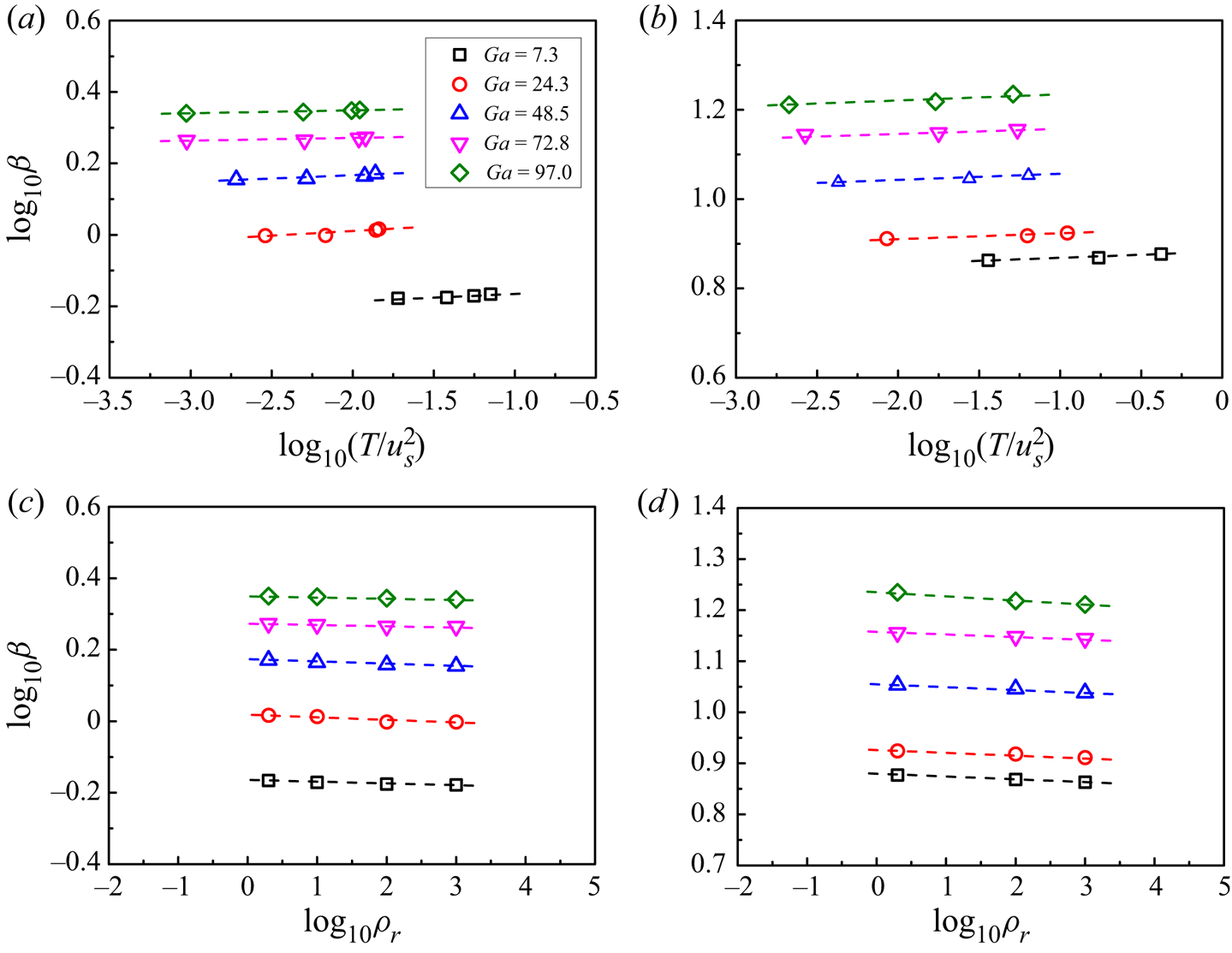
 $\phi =2.36\,\%$ and 14.16 % are shown in figure 8. Our results indicate that
 $\beta$ is insensitive to
 $T/u_s^2$ and the density ratio at the same
 $Ga$, compared to the effects of the particle Reynolds number and the particle volume fraction, although it increases with increasing
 $T/u_s^2$ or decreasing density ratio. Nevertheless, the drag coefficient decreases consistently with increasing density ratio, though not significantly. The maximum difference in the drag for the density ratios 2 and 1000 is more than
 $10\,\%$ for the cases studied, thus it is better to include the density ratio in the drag correlation.
Momentum transfer coefficient  $\beta$ normalized with
 ${\rho _f}{\nu }/d_p^2$ versus normalized granular temperature
 $T/u_s^2$ for (a)
 $\phi =2.36\,\%$, (b)
 $\phi =14.16\,\%$, and versus density ratio for (c)
 $\phi =2.36\,\%$, (d)
 $\phi =14.16\,\%$. Note that for each
 $Ga$, the points (marked by symbols) from left to right correspond to the density ratios changing from 1000 to 2 in (a,b).

We now use our DNS data to establish a new drag correlation in the form of (3.5) and (3.6). We assume that the exponent  $n$ in (3.6) is a function of particle Reynolds number, particle volume fraction and density ratio in the form
 $n(Re_p,\rho _r,\phi ) = (a + b\ln (Re_p))\ln (\phi ^{-1})\,\rho _r^{ - c}$, in which
 $a$,
 $b$ and
 $c$ are constants. The reason for the incorporation of
 $\ln (\phi ^{-1})$ into
 $n$ is that a larger value of
 $n$ is needed to better fit our data for a smaller
 $\phi$ at the same
 $Re_p$ and
 $\rho _r$, and the logarithmic function is tested to be a good choice. The logarithmic functions for
 $\phi$ and
 $Re_p$ were adopted previously by Zaidi (Reference Zaidi2018). From fitting of out data, we obtain the following drag correlation:
 \begin{equation} \left.\begin{gathered} \beta = \frac{3}{4}\,{C_d}\,\frac{{{\rho _f}\phi (1 - \phi )\,|u_s|}}{{{d_p}}}\,{(1 - \phi )^{ - n}}, \\ n = (3.88 - 0.38\ln (Re_p))\ln (\phi^{{-}1})\,\rho_r^{ - 0.038}. \end{gathered}\right\}\end{equation}
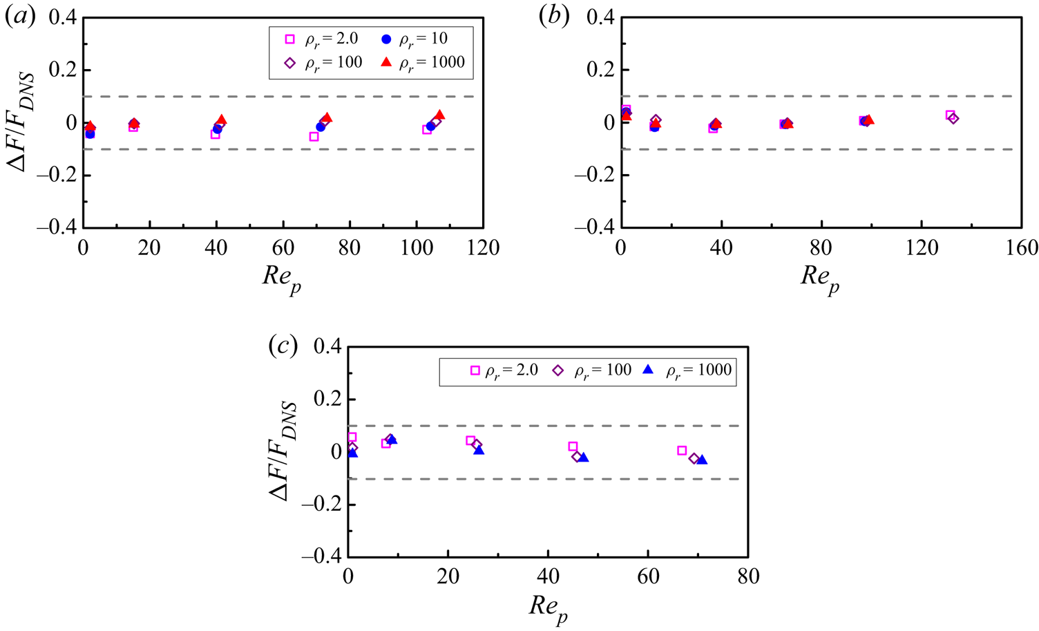
The relative differences between the drag forces from the DNS and from the new drag correlation given by (3.11) for different particle Reynolds numbers and particle volume fractions are plotted in figure 9. It can be seen that the drag correlation is in good agreement with the DNS results, with a maximum relative deviation of around 6 %. Our drag correlation predicts well the drag in the channel centre region of the upward turbulent particle-laden channel flow at relatively high particle Reynolds numbers, where the flow is dominated essentially by the particle sedimentation, as shown in figure 18(a), and also the drag across the channel for the laminar particle-laden channel flow, as shown in figure 25(c) in Appendix A.
Relative differences between the drag forces obtained from the new drag correlation (3.11) and the DNS for (a)  $\phi =0.59\,\%$, (b)
 $\phi =2.36\,\%$, and (c)
 $\phi =14.16\,\%$. Here,
 $\Delta F/{F_{DNS}} = ({F_{D,MOD}} - {F_{D,DNS}})/{F_{D,DNS}}$.

3.3. Microstructure
The drag force is related closely to the microstructure of the particle distribution, thus here we intend to examine the particle microstructure in our sedimentation system through the pair distribution function  $P(\boldsymbol {r})$. In the spherical coordinate frame,
 $P(\boldsymbol {r})$ is defined by (Kulkarni & Morris Reference Kulkarni and Morris2008)
 \begin{equation} P(\boldsymbol{r})=P(r, \theta, \psi)=\frac{H(r, \theta, \psi)}{n t_{s}\,\Delta V}, \end{equation}
where  $\boldsymbol {r}$ is the position vector from the centre of a reference particle to the centre of a neighbouring particle,
 $\theta$ is the polar angle (measured from the positive
 $x$-axis), and
 $\psi$ is the azimuthal angle (measured from the positive
 $z$-axis). Also,
 $H(r, \theta, \psi )$ is the histogram of particle pairs, and
 $\Delta V=r^2\, \Delta r \sin \theta \,\Delta \psi \,\Delta \theta$ is the volume of the sampling bin;
 $n$ is the average particle number density, and
 $t_s$ is the total number of sampling points;
 $P(\boldsymbol {r})$ is axisymmetric about the direction of gravity (i.e. the
 $x$-axis), therefore we need to present
 $P(\boldsymbol {r})=P(r, \theta )$ only by averaging data over
 $\psi$. By further averaging
 $P(r, \theta )$ over
 $\theta$, one obtains the radial distribution function
 $g(r)$ as
 \begin{equation} g(r)=\tfrac{1}{2} \int_{0}^{\rm \pi} P(r, \theta) \sin \theta \,{\rm d} \theta, \end{equation}
which represents the average number of particle pairs with the inter-particle distance ranging from  $r$ to
 $r + \textrm {d} r$, normalized with the average number of particle pairs in the domain.
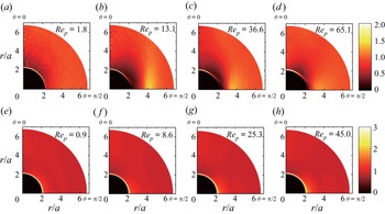
Previous numerical results indicated that the settling particles have an anisotropic microstructure (Yin & Koch Reference Yin and Koch2007, Reference Yin and Koch2008; Alghalibi et al. Reference Alghalibi, Fornari, Rosti and Brandt2020). Figure 10 shows the pair probability distribution functions  $P(r, \theta )$ for
 $\phi =2.36\,\%$ and 14.16 % at
 $\rho _r=2.0$ and different Galileo numbers. For
 $\phi =2.36\,\%$, when the effect of the fluid inertia is significant (i.e.
 $Re_p \ge 13.1$), the probability of a particle pair in near contact is high for the end-to-end configuration and is low for the side-by-side configuration, as shown in figures 10(b–d). Yin & Koch (Reference Yin and Koch2007) observed a decreased pair distribution function for pairs with vertical separation, and a peak in the pair distribution function for horizontal separations corresponding to about two particle diameters, as a result of the wake effect. Similar results can be seen in figures 10(b–d). Our results indicate that the anisotropy in
 $P(r, \theta )$ first intensifies and then weakens, as
 $Ga$ or
 $Re_p$ increases. By contrast, at a relatively high volume fraction of
 $\phi =14.16\,\%$, the above anisotropic microstructure disappears: the probability of a particle pair in near contact is high in all directions, and the pair distribution function is nearly homogeneous elsewhere, due presumably to the strong interactions (e.g. collisions) between the particles.
Pair distribution functions  $P(r,\theta )$ for (a–d)
 $\phi =2.36\,\%$ and (e–h)
 $\phi =14.16\,\%$, at
 $\rho _r=2.0$. The Galileo numbers are
 $Ga=7.3$, 24.3, 48.5, 72.7 from left to right.

Figure 11 shows the particle pair distribution for  $\rho _r=10 - 1000$ and the radial distribution functions for
 $\rho _r=2 - 1000$ at
 $Ga=24.3$. Comparison between figures 10(b,f) and figures 11(a,b,d,e) indicates that the particle pair distribution tends to become more homogeneous as the density ratio increases, as can also be seen directly from figures 11(c,f) for the radial distribution functions
 $g(r)$.
Pair distribution functions  $P(r,\theta )$ for (a)
 $(\rho _r, \phi )=(10, 2.36\,\%)$, (b)
 $(\rho _r, \phi )=(100, 2.36\,\%)$, (d)
 $(\rho _r, \phi )=(100, 14.16\,\%)$, and (e)
 $(\rho _r, \phi )=(1000, 14.16\,\%)$, at
 $Ga=24.3$, and radial distribution functions
 $g(r)$ for (c)
 $\phi =2.36\,\%$, and (f)
 $\phi =14.16\,\%$, at
 $Ga=24.3$.

The drag may be affected by the clustering of the particles (Tavanashad et al. Reference Tavanashad, Passalacqua and Subramaniam2021). From figures 10 and 11, large-scale closely packed particle clusters do not form in our simulations, since there is no local peak for the pair distribution function at  $r/d_p=2$ and 3 (i.e.
 $r/a=4$ and 6). This is confirmed by checking directly the particle distribution in our simulations. Thus we think that our sedimentation system is homogeneous as a whole. We note that Uhlmann & Doychev (Reference Uhlmann and Doychev2014) observed strong clustering of particles in the form of vertically elongated columnar regions at
 $Ga=178$. The highest Galileo number is 121 for our simulations, and at this
 $Ga$, no clustering was observed by Uhlmann & Doychev (Reference Uhlmann and Doychev2014).
4. Modelling interphase drag of upward turbulent particle-laden channel flows
To our knowledge, no drag correlation has been developed to account for the turbulence effect, although the effects of the turbulence on the drag force or the particle settling velocity in isotropic turbulence have been investigated (Good et al. Reference Good, Ireland, Bewley, Bodenschatz, Collins and Warhaft2014; Fornari et al. Reference Fornari, Picano and Brandt2016a,Reference Fornari, Picano, Sardina and Brandtb). Here, we intend to develop a new drag correlation by modelling the drag of upward turbulent particle-laden channel flows simulated by Yu et al. (Reference Yu, Xia, Guo and Lin2021). The schematic diagram of the flow is shown in figure 12. The computational domain is  $[0, 8H] \times [0, 2H] \times [0, 4H]$ in the streamwise (
 $x$), wall-normal (
 $y$) and spanwise (
 $z$) directions, respectively, where
 $H$ is the half-width of the channel. The periodic boundary condition is imposed in the streamwise and spanwise directions, and the no-slip velocity boundary condition is imposed on the side walls. The channel Reynolds number
 $Re_b= 2u_b H/ \nu$ is kept constant by adjusting a time-dependent pressure gradient
 $\mathrm {d} p_{e} / \mathrm {d} x$ in the
 $x$-direction, where
 $u_b$ is the bulk velocity.
Schematic diagram of the upward particle-laden channel flow studied by Yu et al. (Reference Yu, Xia, Guo and Lin2021), where  $x$,
 $y$ and
 $z$ represent the streamwise, transverse and spanwise coordinates, respectively.

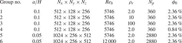
As shown in table 4, the data used in the present work were obtained from the simulations for six groups of parameters (Yu et al. Reference Yu, Xia, Guo and Lin2021). A dimensionless parameter  $u_i/u_b$, defined as the settling coefficient, is introduced to control the particle settling effect, where
 ${u_i} = \sqrt {8a({\rho _r} - 1)g/3}$. For each group, the settling coefficient is varied to yield different slip velocities and particle Reynolds numbers. For a given value of
 $u_i/u_b$, the Galileo number can be computed from
 \begin{equation} Ga=\frac{\sqrt{3}}{2}\,\frac{a}{H}\,\frac{u_{i}}{u_{b}}\,Re_{b}. \end{equation}
Physical and computational parameters of the DNS database for the particle-laden flows (Yu et al. Reference Yu, Xia, Guo and Lin2021). Here,  $a$ is the particle radius,
 $N_p$ is the total number of particles, and
 $\phi _{{0}}$ is the mean particle volume fraction in the whole channel.

It should be noted that for the channel flow here, the averaging is performed in the streamwise ( $x$) and spanwise (
 $y$) directions, and over time at the statistically steady state, thus the mean quantity is a function of the wall-normal position (i.e.
 $y$-coordinate). The particle volume fraction
 $\phi (y)$ is calculated as the percentage of the grids at
 $y$ covered by the particle domain for all averaging samples, which is a good method because we use a homogeneous grid spacing over the channel. The particle volume fraction for the entire channel is denoted by
 $\phi _{{0}}$.
4.1. Slip velocity
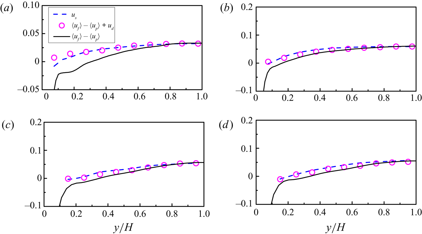
Any drag model involves the slip velocity. For the discrete particle method, the slip velocity is defined as the difference between the particle velocity and the fluid velocity at the particle position, whereas for the two-fluid model, the slip velocity is defined typically as the difference between two phase-averaged velocities. It is a difficult issue how to evaluate properly the slip velocity from the interface-resolved simulations, since on the one hand, the slip velocity vanishes on the particle surface, which causes difficulty in providing the slip velocity for the discrete particle method, and on the other hand, the difference between two phase-averaged velocities in a specific domain may not reflect the difference between the mean velocities in a local domain, which introduces the concept of the drift velocity (Capecelatro, Desjardins & Fox Reference Capecelatro, Desjardins and Fox2016; Baker et al. Reference Baker, Fox, Kong, Capecelatro and Desjardins2020) that needs to be modelled for the two-fluid model.
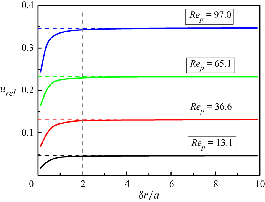
The effective slip velocity for an individual particle may be defined as the relative velocity of the fluid located a few particle radii away from the particle surface. The relative velocity was calculated from the fluid velocity averaged over a spherical shell surrounding the particle for the isotropic turbulence (Cisse, Homann & Bec Reference Cisse, Homann and Bec2013; Fornari et al. Reference Fornari, Picano and Brandt2016a), and from the fluid velocity averaged over a cut shell for the turbulent channel flow (Kidanemariam et al. Reference Kidanemariam, Chan-Braun, Doychev and Uhlmann2013; Zhu et al. Reference Zhu, Yu, Shao and Deng2020b). Figure 13(a) shows a two-dimensional schematic diagram of the cut shell, which is a part of a spherical shell of thickness  $\varDelta =a/4$ (
 $a$ being the particle radius) between two planes located at
 $y_0 \pm d_{y}$, where
 $y_0$ is the
 $y$-position of the particle centre, and
 $d_y$ is the half-width of the averaging domain. Following Zhu et al. (Reference Zhu, Yu, Shao and Deng2020b),
 $d_y=0.25a$ is chosen in the present study. We calculate the relative velocity as a function of the distance between the cut shell and the particle,
 $\delta _r$, as
 \begin{equation} {\boldsymbol{u}_{rel}} = \left\langle {\int_{\varOmega (\delta r)} {\frac{1}{{\varOmega (\delta r)}}}\,{\boldsymbol{u}_f}\,{\rm{d}}V - {\boldsymbol{u}_p}} \right\rangle, \end{equation}
where  $\varOmega (\delta r)$ is the volume of the cut shell with the distance between the cut shell and the particle being
 $\delta r$, and the data are averaged for all particles in a specific
 $y$-band. The average fluid and particle velocities in the wall-normal and spanwise directions are zero, and we are concerned with only the streamwise component of
 ${\boldsymbol {u}_{rel}}$, defined by
 $u_{rel}$.
(a) Two-dimensional schematic diagram of the computational model for the relative mean velocity;  $\delta r$ is the distance between the shell and the particle surface, and
 $\varDelta$ is the thickness of the spherical shell. (b) Relative mean velocities of the fluid in a cut shell of thickness
 $a/4$ with respect to the particle as a function of the distance between the shell and the particle surface for different
 $y$-bands at
 $(a/H,\rho _r,Re_b,\phi _0, u_i/u_b)=(0.05,2,5746,2.36\,\%,0.092)$. The averaging is performed for the particles located in each
 $y$-band, and in the legend, ‘0.05–0.1’ means the
 $y$-band
 $0.05H < y < 0.1H$. (c) Comparison between the relative mean velocities at
 $\delta r/a=1.0$, 2.0 and 3.0, and the interphase mean velocity difference
 $\langle {u_f}\rangle -\langle u_p\rangle$. (d) Drag predictions from (3.5)–(3.11) with different relative mean velocities. The inset shows the close-up near the wall.

Figure 13(b) shows the relative mean velocities  $u_{rel}$ as a function of the distance between the cut shell and the particle for the typical case
 $(a/H,\rho _r,Re_b,\phi _0,u_i/u_b)= (0.05,2,5746,2.36\,\%,0.092)$. The relative mean velocity
 $u_{rel}$ first increases with increasing distance away from the particle surface (
 $\delta r$). For the channel centre region at roughly
 $y/H>0.7$,
 $u_{rel}$ reaches a constant value around
 $\delta r > 3a$, whereas for the other region,
 $u_{rel}$ decreases with increasing
 $\delta r$ after reaching its maximum, as shown in figure 13(b). For the upward turbulent channel flows at a relatively small settling coefficient (e.g.
 $u_i/u_b=0.092$ here), the particle volume fraction
 $\phi _s$ in the near-wall region is lower than in the bulk region due to the Saffman effect, and the particles tend to be located in the fluid high-speed streaks, due to the entrainment of the particles by the streamwise vortex pairs (Zhu et al. Reference Zhu, Yu, Pan and Shao2020a), which results in the decrease of
 $u_{rel}$ with increasing
 $\delta r/a$.
Thus a suitable choice of  $\delta r$ is necessary to determine the effective slip velocity and for modelling the interphase drag force. Cisse et al. (Reference Cisse, Homann and Bec2013) argued that the fluid–particle coupling takes place mainly at distances of the order of
 $d_p$ for finite-size neutrally buoyant particles in turbulence. Fornari et al. (Reference Fornari, Picano and Brandt2016a) performed a parametric study on the slip velocity for spheres settling in an isotropic turbulence field by changing the inner radii of the spherical shells, and an inner radius
 $3.5a$ was selected to compute the slip velocity.
Figure 13(c) shows the comparison of the relative mean velocities at  $\delta r/a=1$, 2 and 3, and the interphase mean velocity difference
 $\langle {u_f}\rangle -\langle u_p\rangle$. Clearly, the relative mean velocity
 $u_{rel}$ is dependent on
 $\delta r/a$, particularly in the near-wall region. In figure 13(d), we compare the drag predictions from (3.5)–(3.11) using the relative mean velocities
 $u_{rel}$ at
 $\delta r/a=1$, 2 and 3. The drag prediction obtained using the interphase mean velocity difference is also plotted for comparison. It is observed in the inset of figure 13(d) that an inappropriate
 $\delta r$ may lead to an opposite direction of the drag force: for
 $\delta r/a=1$, the predicted drag force is positive at
 $y/H=0.075$, but the DNS drag is negative, and for
 $\delta r/a=3$, the predicted drag force is negative at
 $y/H=0.125$, but the DNS drag is positive. Therefore, we choose the relative velocity at
 $\delta r=2a$ as the effective slip velocity
 $u_s$ that is used directly in the drag correlation, i.e.
 \begin{equation} u_s={\left. {{u_{rel}}} \right|_{\delta r/a = 2}}, \end{equation}
which ensures that the direction of the predicted drag is consistent with that of the DNS drag for the above case. At the moment, we do not know how to determine the optimal  $\delta r$ for the effective slip velocity, which is a subject worthy of further study.
Note that we take the interphase mean velocity difference for the entire domain  $\langle {u_f}\rangle -\langle u_p\rangle$ as the effective slip velocity for the sedimentation problem studied in the previous section. In figure 14, we plot the relative mean velocity as a function of
 $\delta r/a$ at different density ratios for the sedimentation problem. It is not surprising that for each case, the relative velocity increases monotonically to
 $\langle {u_f}\rangle -\langle u_p\rangle$, like the relative velocity in the channel centre region for the upward channel flow in figure 13(b). The relative velocity at
 $\delta r=2a$ is close to
 $\langle {u_f}\rangle -\langle u_p\rangle$, with approximately 1.5 % relative difference. It is better to take the relative velocity at
 $\delta r=3a$ as the slip velocity for the homogeneous system without the drift velocity, but
 $\delta r=2a$ may be a better choice for the case where the drift velocity occurs, as discussed earlier.
Relative mean velocity  $u_{rel}$ as a function of the distance to the particle surface at
 $(\phi,\rho _r)=(2.36\,\%,2.0)$ for the particle sedimentation in a periodic box. The dashed lines represent the corresponding interphase mean velocity differences.

4.2. Drag correlation
The fluid-phase mean momentum equation in the streamwise direction for the channel flow at the statistically stationary state reads (Yu et al. Reference Yu, Lin, Shao and Wang2017)
 \begin{equation} \frac{{\rm{d}}}{{{\rm{d}}y}}\left( {{\phi _f}\mu\,\frac{{{\rm{d}}\langle {{u_f}} \rangle }}{{{\rm d} y}}} \right) + {\phi _f}\left( { - \frac{{{\rm{d}}{p_e}}}{{{\rm{d}}x}}} \right) + \frac{{\rm{d}}}{{{\rm{d}}y}}\left( {{\phi _f}{\rho _f}\left\langle { - {{u'}_f}{{v'}_f}} \right\rangle } \right) - F_D = 0, \end{equation}
where  $F_D$ is the drag force on the particles per unit volume, averaged in the streamwise and spanwise directions and over time. Here,
 $\phi _f$ and
 $\phi _s$ are the fluid and solid volume fractions at a given
 $y$-position, respectively. The DNS drag force is then computed from
 \begin{equation} {F_D} = \frac{{\rm{d}}}{{{\rm{d}}y}}\left( {{\phi _f}\mu\,\frac{{{\rm{d}}\langle {{u_f}} \rangle }}{{{\rm d} y}}} \right) + {\phi _f}\left( { - \frac{{{\rm{d}}{p_e}}}{{{\rm{d}}x}}} \right) + \frac{{\rm{d}}}{{{\rm{d}}y}}\left( {{\phi _f}{\rho _f}\left\langle { - {{u'}_f}{{v'}_f}} \right\rangle } \right). \end{equation}
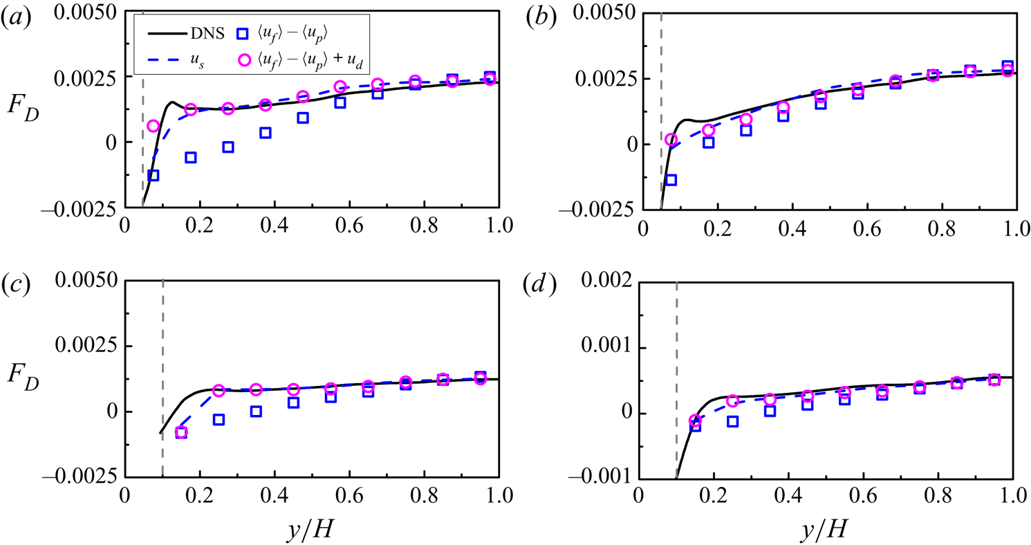
Figure 15 presents a comparison between the interphase drag forces obtained from the DNS data and the drag correlation (3.11), with the relative mean velocity at  $\delta r=2a$ as the effective slip velocity. We note that the particle Reynolds number
 $Re_p$ shown in the legends is based on the slip velocity at the channel centre. From figure 15, the drag correlation underestimates significantly the drag force, particularly for relatively low
 $Re_p$ and the near-wall region. The drag underestimation is caused mainly by the turbulence effect, as observed in the isotropic turbulence laden with finite-size particles (Fornari et al. Reference Fornari, Picano and Brandt2016a,Reference Fornari, Picano, Sardina and Brandtb). We define the drag force predicted by (3.11) in the absence of background turbulence as
 $F_{D0}$. The relative increase in the drag due to the turbulence effect is defined as
 \begin{equation} \psi = \frac{{{F_D} - {F_{D0}}}}{{{F_{D0}}}}, \end{equation}
where  $F_D$ is the DNS drag from the interfaced-resolved simulation of the upward turbulent channel. It is shown in figure 25 in Appendix A that the drag correlation (3.11) can predict well the drag for the laminar particle-laden channel flow, therefore the difference between
 $F_D$ and
 $F_{D0}$ is caused mainly by the turbulence effect.
Comparison between the interphase drags  $F_D$ obtained from the DNS data (4.5) represented by solid lines and the drag correlation (3.11) without turbulence correction represented by symbols for (a)
 $(a/H,\rho _r,Re_b,\phi _0)=(0.05,2,5746,2.36\,\%)$, (b)
 $(a/H,\rho _r,Re_b,\phi _0)=(0.05,2,12\,000,2.36\,\%)$, (c)
 $(a/H,\rho _r, Re_b,\phi _0)=(0.1,2,5746,2.36\,\%)$, (d)
 $(a/H,\rho _r,Re_b,\phi _0)=(0.1,2,5746,0.84\,\%)$, (e)
 $(a/H,\rho _r,Re_b,\phi _0)= (0.1,10,5746,2.36\,\%)$, and (f)
 $(a/H,\rho _r,Re_b,\phi _0)=(0.1,100,5746,2.36\,\%)$. Here,
 $F_D$ is normalized by
 $\rho _f u^2_b/H$, and
 $Re_p$ is the particle Reynolds number based on mean slip velocity at the channel centre. The horizontal dashed lines represent zero force for reference, and the vertical dashed lines represent the position where the particles touch the wall.

Homann et al. (Reference Homann, Bec and Grauer2013) studied the effect of the turbulence intensity on the drag on a fixed sphere. The results indicated that the relative increase in the drag was proportional to  $C(Re_p)I^2$, where
 $C(Re_p)$ is a function of the particle Reynolds number, and
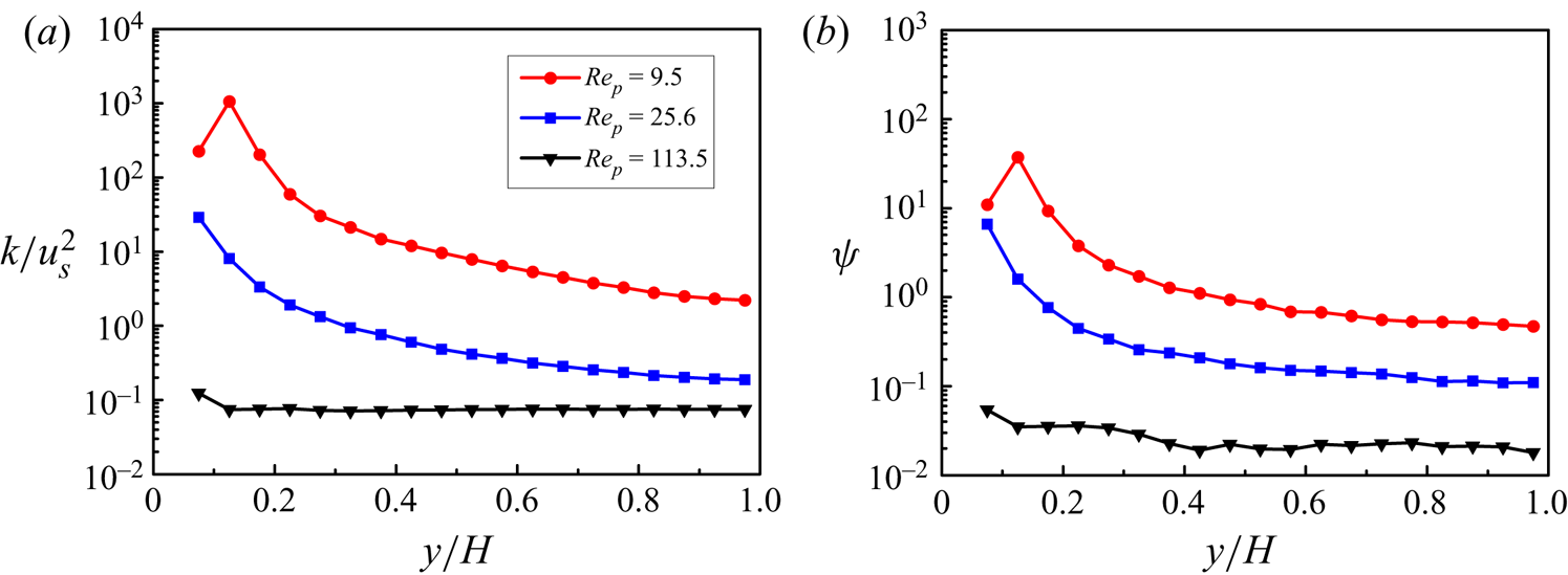
 $I=u'/u_s$ is the relative turbulence intensity. Similar results were observed in the simulations of the particle-laden isotropic turbulent flows (Chouippe & Uhlmann Reference Chouippe and Uhlmann2015; Fornari et al. Reference Fornari, Picano, Sardina and Brandt2016b). Thus here we incorporate the relative turbulence intensity or similarly the relative turbulent kinetic energy (TKE) into our drag correlation to account for the turbulence effect. Figure 16(a) plots the profiles of the relative TKE (
 $k/u_s^2$) for
 $(a/H,\rho _r,Re_b,\phi _0)=(0.05,2,5746,2.36\,\%)$ at different particle Reynolds numbers, and figure 16(b) presents the relative difference between the DNS drag of the turbulent channel flow and the drag correlation (3.11),
 $\psi$, for the same cases. Comparison between figures 16(a) and 16(b) confirms that there is a strong correlation between the relative TKE
 $k/u_s^2$ and the relative drag increase induced by turbulence.
(a) Profiles of TKE normalized by the square of the mean slip velocity  $u_s$ for the turbulent channel flow. (b) Relative difference between the DNS drag and the drag correlation (3.11) for
 $(a/H,\rho _r,Re_b,\phi _0)=(0.05,2,5746,2.36\,\%)$.

From (4.6), we have
 \begin{equation} {F_D} = (1 + \psi ){F_{D0}} = \frac{3}{4}\,(1 + \psi ){C_d}\,\frac{{{\rho _f}{\phi}{\phi _f}\left| {{u_s}} \right|{u_s}}}{{{d_p}}}\,{\phi _f}^{ - n}. \end{equation}
The turbulence correction  $\psi$ needs to be modelled.
It should be noted that normally, the wall effect on the drag force is important (Lattanzi, Yin & Hrenya Reference Lattanzi, Yin and Hrenya2020), but this effect is not important here because the particle concentration near the wall is low due to the particle migration away from the wall as a result of the Saffman-type lift force for the upward channel flow studied (Yu et al. Reference Yu, Xia, Guo and Lin2021), thus the volume-averaged drag force near the wall is small for most cases considered. In the present study, the data in the wall region of  $y/H<0.2$ are not used to correlate the turbulence correction of the drag.
Based on our DNS data (Yu et al. Reference Yu, Xia, Guo and Lin2021), we propose two correlations in the present study. One has the following simple correlation for  $\psi$:
 \begin{equation} \psi = 0.448{[k/u_s^2 - (k/u_s^2)_0]^{0.525}}, \end{equation}
where  $k$ is the fluid TKE, and
 $(k/u_s^2)_0$ represents the particle-induced TKE (or the pseudo-TKE) that exists for the laminar particle-laden flows or the turbulent particle-laden flows at high particle Reynolds numbers so that the flow is essentially dominated by particle sedimentation. In Appendix B, we show that
 $(k/u_s^2)_0$ is a function of mainly particle volume fraction at high particle Reynolds numbers for
 $0.59\,\% \le \phi \le 14.16\,\%$:
 \begin{equation} (k/u_s^2 )_0 \approx 0.0125 + 2.15\phi - 5.83\phi^2. \end{equation}
We note that the correlation (4.9) for  $(k/u_s^2)_0$ may not be accurate, but its accuracy is not so important, since its value for the laminar flow is much smaller than that in the presence of background turbulence at relatively small
 $Re_p$. From figure 16(a),
 $k/u_s^2$ for
 $Re_p=9.5$ can be larger than that for
 $Re_p=113.5$ by several orders in magnitude. The turbulence correction
 $\psi$ is significant when
 $k/u_s^2$ is large for the turbulent channel flows at relatively small
 $Re_p$, and negligibly small when the flow is dominated by particle sedimentation at high
 $Re_p$. The correlation (4.9) applies only to the case of low particle volume fractions at relatively high particle Reynolds numbers, and we note that Mehrabadi et al. (Reference Mehrabadi, Tenneti, Garg and Subramaniam2015) proposed the following general correlation for the particle-induced TKE:
 \begin{equation} (k/u_s^2 )_0=\phi + 1.25\phi (1 - \phi )^3 \exp(- \phi\,Re_m^{1/2} ) \end{equation}
for  $0.1 \leqslant \phi \leqslant 0.5$ and
 $0.01 \leqslant Re_m \leqslant 300$. Here,
 $Re_m=(1 - \phi ) Re_p$. The correlation (4.10) was obtained from the simulations of the flow over fixed spheres, but was shown to be applicable to the freely evolving suspension (Mehrabadi et al. Reference Mehrabadi, Tenneti, Garg and Subramaniam2015). Our correlation (4.9) predicts a higher relative TKE than that by (4.10), e.g. 0.2 versus 0.172 for
 $\phi =0.14$ and
 $Re_m=80$. One reason for the difference is the effect of the computational domain: we adopt a rectangular domain of
 $40{d_p} \times 20{d_p} \times 20{d_p}$, whereas Mehrabadi et al. (Reference Mehrabadi, Tenneti, Garg and Subramaniam2015) used a cubic domain with maximum length
 $7.5d_p$. The difference is reduced when we decrease the domain size. In addition, the correlation (4.10) seemed to underpredict the DNS result at
 $\phi =0.1$ and
 $Re_m=80$, from figure 12 in Mehrabadi et al. (Reference Mehrabadi, Tenneti, Garg and Subramaniam2015).
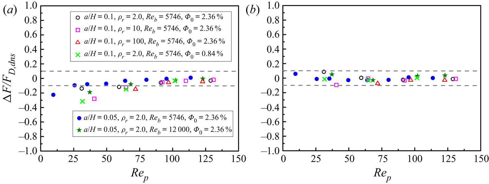
Figure 17 shows the comparison between the drags  $F_D$ obtained from the DNS data (4.5) and the drag correlation with turbulence correction (4.7)–(4.8) for different simulation cases. Our drag correlation can predict well the interphase drags for different particle sizes, density ratios, bulk Reynolds numbers and particle volume fractions. Figure 18 compares the relative difference between the DNS drag and the drag correlations with and without turbulence corrections at the channel centre. This comparison and the comparison between figures 15 and 17 show that our drag correlation with turbulence correction (4.8) improves significantly the prediction accuracy, particularly for relatively low particle Reynolds numbers.
Comparison between the interphase drags  $F_D$ obtained from the DNS data (4.5) and the drag correlation with turbulence correction (4.7)–(4.8), for (a)
 $(a/H,\rho _r,Re_b,\phi _0)=(0.05,2,5746,2.36\,\%)$, (b)
 $(a/H,\rho _r,Re_b,\phi _0)=(0.05,2,12\,000,2.36\,\%)$, (c)
 $(a/H,\rho _r,Re_b,\phi _0)=(0.1,2,5746,2.36\,\%)$, (d)
 $(a/H,\rho _r, Re_b,\phi _0)=(0.1,2,5746,0.84\,\%)$, (e)
 $(a/H,\rho _r,Re_b,\phi _0)=(0.1,10,5746,2.36\,\%)$, and (f)
 $(a/H,\rho _r, Re_b, \phi _0)=(0.1,100,5746,2.36\,\%)$. The solid lines and the symbols represent the drags from DNS and the correlation, respectively, and
 $F_D$ is normalized by
 $\rho _f u^2_b/H$. The vertical dashed lines represent the position where the particles touch the wall.

Relative difference between the DNS drag and (a) the drag correlation without turbulence correction, and (b) the drag correlation with turbulence correction (4.8) at the channel centre.

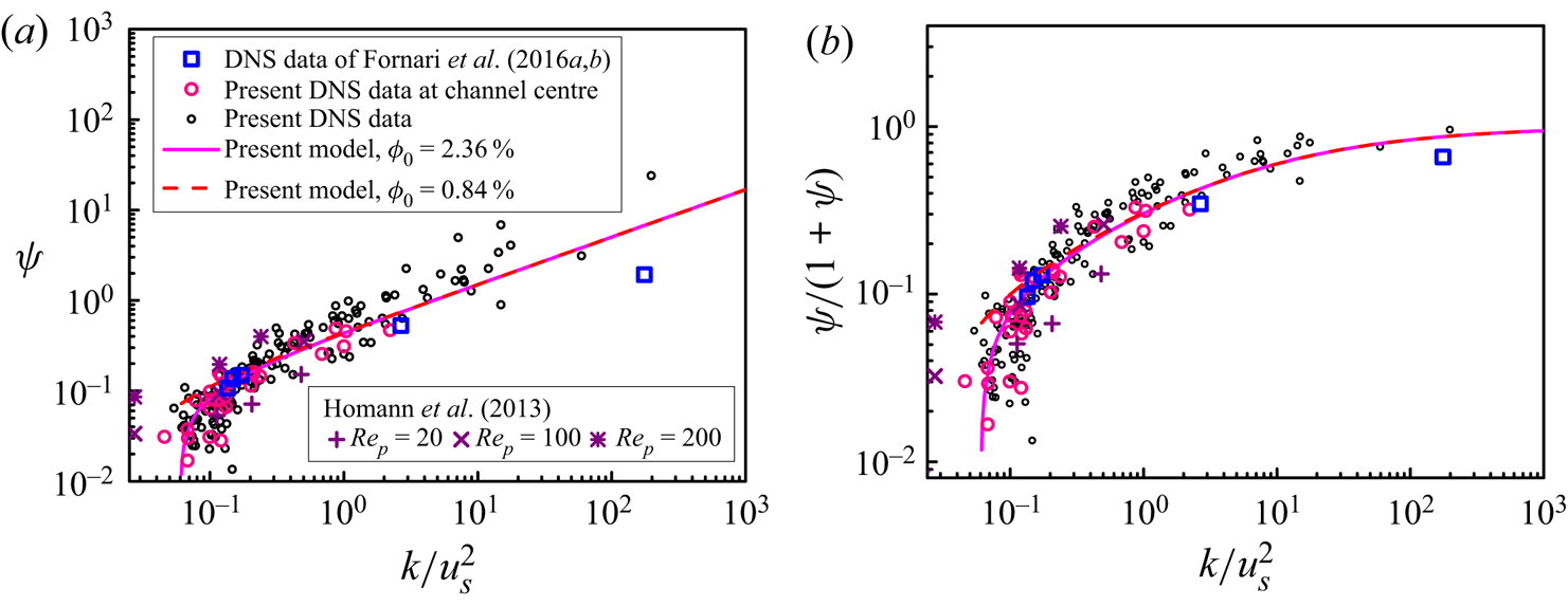
The drag correlation (4.7)–(4.8) is established from our DNS data for the upward turbulent channel flow, and it remains to be seen whether it can predict well the drag for other flows. There are no experimental data available for the validation of the drag model for the turbulent particle-laden flow. Here, we compare our drag correction to the DNS results of Fornari et al. (Reference Fornari, Picano and Brandt2016a,Reference Fornari, Picano, Sardina and Brandtb) on the particle sedimentation in isotropic turbulence at  $Ga = 19$, 60, 145 and 200 for
 $\phi _0 = 0.5- 1\,\%$, and the DNS results of Homann et al. (Reference Homann, Bec and Grauer2013) on the flow over a fixed particle at
 $Re_p=20$, 100 and 200. The turbulence correction
 $\psi$ and the relative contribution of the turbulence to the total drag
 $\psi /(1 + \psi )$ (i.e.
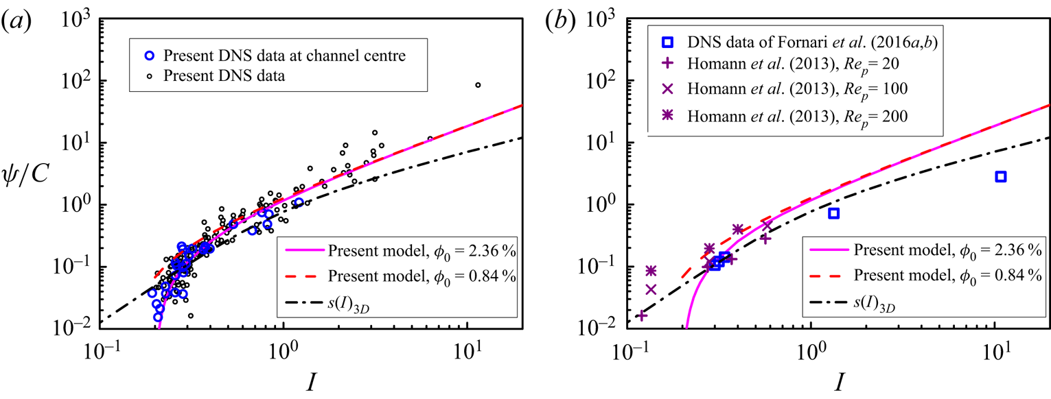
 $({F_D} - {F_{D0}})/F_D$) from the present correlation (4.8), and the DNS data of Fornari et al. (Reference Fornari, Picano and Brandt2016a,Reference Fornari, Picano, Sardina and Brandtb), Homann et al. (Reference Homann, Bec and Grauer2013) and the present study are compared in figure 19. Our correlation (4.8) and the DNS results are in fairly good agreement with those of Fornari et al. (Reference Fornari, Picano and Brandt2016a,Reference Fornari, Picano, Sardina and Brandtb) and Homann et al. (Reference Homann, Bec and Grauer2013). In figure 19, we distinguish our DNS data between the channel centre and the non-centre region. The turbulence at the channel centre is nearly isotropic. Figure 19 implies that the shear turbulence and the isotropic turbulence have similar effects on the drag at least for relatively low
 $k/u_s^2$.
(a) The turbulence correction  $\psi$, and (b) the relative contributions of the turbulence to the total drag from the present correlation (4.8), as compared to the DNS data of Fornari et al. (Reference Fornari, Picano and Brandt2016a,Reference Fornari, Picano, Sardina and Brandtb) on the particle sedimentation in isotropic turbulence and the DNS results of Homann et al. (Reference Homann, Bec and Grauer2013) on the flow over a fixed particle. The present DNS data at the channel centre and off-centre positions are also shown.

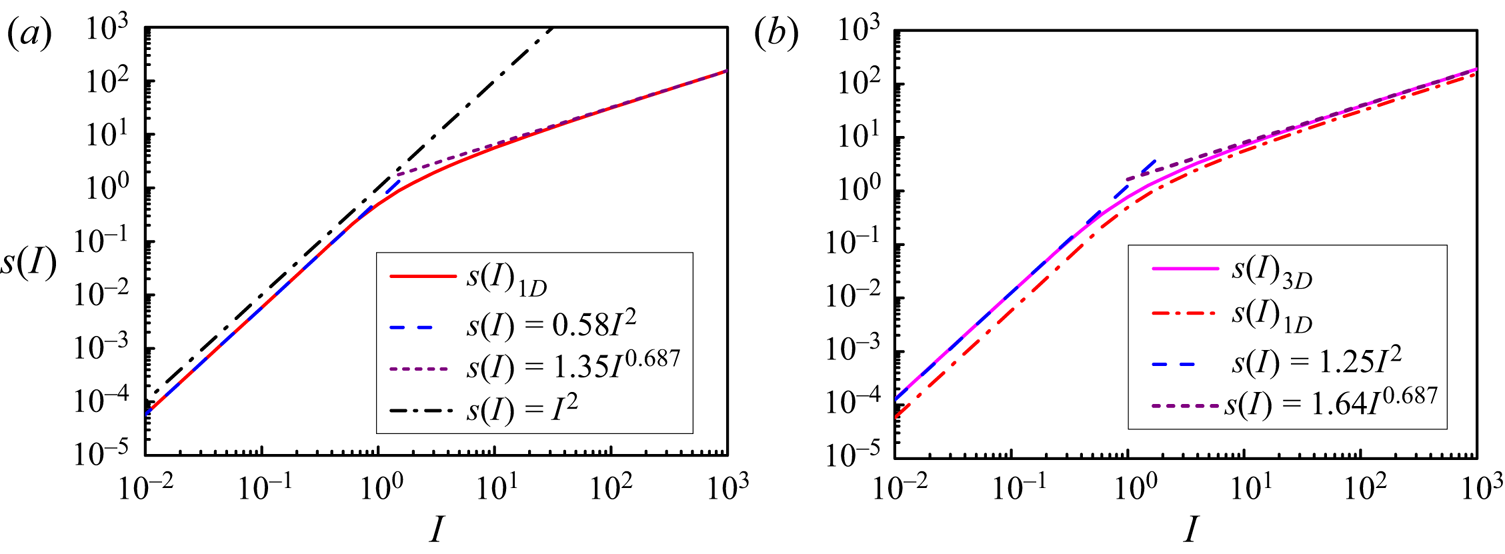
As mentioned earlier, Homann et al. (Reference Homann, Bec and Grauer2013) observed that the relative increase in the drag on a fixed sphere due to the background turbulence was proportional to the square of the relative turbulence intensity  $I^2$ (i.e. the relative TKE), whereas from (4.8), the relative increase for our particle-laden turbulent flow is almost linearly proportional to the relative turbulence intensity
 $I$. In the following, we attempt to explain the discrepancy and provide our second turbulence correlation of the drag.
Following Homann et al. (Reference Homann, Bec and Grauer2013), we assume that a particle is fixed in an incoming turbulent flow, whose velocity  ${\boldsymbol {u}}$ is approximated by a Gaussian random distribution with mean velocity
 $u_s{\boldsymbol {e}}_x$ (where
 ${\boldsymbol {e}}_x$ is a unit vector pointing in the mainstream direction) and variance
 $u_{rms}^2$ in each direction, and the instantaneous slip velocity is equal to the fluid velocity. Thus the instantaneous drag force on the particle can be approximated as
 \begin{equation} {\boldsymbol{F}} = 6{\rm \pi} a\mu {\boldsymbol{u}}\left[1 + 0.15\left( {\frac{{d_p \left| {\boldsymbol{u}} \right|} }{\nu }} \right)^{0.687}\right]. \end{equation}
Here, we consider two cases: one is a one-dimensional model for which we assume that the fluctuating velocity is parallel to the mean velocity without the lateral components, and the other is a three-dimensional model for which the fluctuating velocity in each direction is independently and identically distributed with a Gaussian probability density function. The mean drags on the particle can be evaluated by, respectively,
 \begin{equation} (F_D)_{1D} = \frac{{6{\rm \pi} a\mu } }{{\sqrt {2{\rm \pi} }\,u_{rms} }}\int_{ - \infty }^\infty {u\left[1 + 0.15\left( {Re_p\,\frac{{\left| u \right|} }{{u_s }}} \right)^{0.687} \right]\exp\left( { - \frac{{\left( {u - u_s } \right)^2 } } {{2u_{rms}^2 }}}\right){\rm{d}}u} \end{equation}
and
 \begin{align} (F_D )_{3D} &= \frac{{6{\rm \pi} a\mu } }{{(\sqrt {2{\rm \pi} }\,u_{rms} )^3 }}\int {\int {\int {u\left[1 + 0.15 \left( {Re_p\,\frac{{\sqrt {u^2 + v^2 + w^2 } } }{{u_s }}} \right)^{0.687} \right]} } } \nonumber\\ &\quad\times\exp \left( { - \frac{{\left( {u{{ - }}u_{{s}} } \right)^{{2}} } } {{{{2}}u_{{{rms}}}^{{2}} }}} \right)\exp \left( { - \frac{{v^{{2}} } }{{{{2}}u_{{{rms}}}^{{2}} }}} \right)\exp \left( { -\frac{{w^{{2}} } } {{{{2}}u_{{{rms}}}^{{2}} }}} \right){\rm{d}}u\,{\rm{d}}v\,{\rm{d}}w. \end{align}
For the one-dimensional model, one can derive the relative increase in the drag due to the fluctuating velocity:
 \begin{align} \psi_{1D} &= \frac{{F_D - F_{D0} } }{{F_{D0} }} \nonumber\\ &= \frac{{0.15Re_p^{0.687} \left[ {\dfrac{1 }{{\sqrt {2{\rm \pi} }\,I}}\displaystyle\int {\dfrac{u }{{u_s }}\left( {\dfrac{{\left| u \right|} } {{u_s }}} \right)} ^{0.687} \exp\left( { - \dfrac{{\left( {u/u_s - 1} \right)^2 } }{{2I^2 }}} \right){\rm{d}}\left( {\dfrac{u }{{u_s }}} \right) - 1} \right]}}{{1 + 0.15\,Re_p^{0.687} }}, \end{align}
where  $I$ represents the relative turbulence intensity, defined as
 $I=u_{rms}/u_s$. By defining
 \begin{equation} s(I)_{1D} = \frac{1 }{{\sqrt {2{\rm \pi} }\,I}}\int_{ - \infty }^\infty {x\left| x \right|^{0.687} \exp\left( { - \frac{{\left( {x - 1} \right)^2 } }{{2I^2 }}} \right){\rm{d}}x - 1} \end{equation}
and
 \begin{equation} C(Re_p ) = \frac{{0.15\,Re_p^{0.687} } }{{1 + 0.15\,Re_p^{0.687} }}, \end{equation}
(4.14) can be simplified as
 \begin{equation} \psi_{1D}= C(Re_p)\,s(I)_{1D}. \end{equation}
Similarly, one can derive the relative increase in the drag due to the fluctuating velocity for the three-dimensional model:  $\psi _{3D}= C(Re_p)\,s(I)_{3D}$, and
 \begin{align} s(I)_{3D} &= \frac{1 }{{(\sqrt {2{\rm \pi} }\,I)^3 }}\int {\int {\int {x\left( {\sqrt {x^2 + y^2 + z^2 } } \right)^{0.687} } } } \nonumber\\ &\quad\times \exp\left( { - \frac{{\left( {x - 1} \right)^2 } }{{2I^2 }}} \right)\exp\left( { - \frac{{y^2 } }{{2I^2 }}} \right)\exp\left( { - \frac{{z^2 } }{{2I^2 }}} \right){\rm{d}}x\,{\rm{d}}y\,{\rm{d}}z - 1. \end{align}
Since the explicit expressions for  $s(I)_{1D}$ (4.15) and
 $s(I)_{3D}$ (4.18) cannot be obtained, numerical integration is used to determine
 $s(I)$. The results are shown in figure 20, which indicates that
 $s(I)_{1D}$ can be approximated by
 $s(I)_{1D}=0.58I^2$ at
 $I<1$ and
 $s(I)_{1D}=1.35I^{0.687}$ at
 $I>50$, whereas
 $s(I)_{3D}$ can be approximated by
 $s(I)_{3D}=1.25I^2$ at
 $I<1$ and
 $s(I)_{3D}=1.64I^{0.687}$ at
 $I>50$. Here,
 $s(I)=I^2$ if the integral kernel in (4.15) is
 $x^2$. Our test showed that
 $s(I)$ is proportional to
 $I^2$ for any power exponent
 $m$ in the kernel
 $x\,| x |^m$ for
 $0< m<1$ and
 $I<1$, with a lower coefficient for a smaller
 $m$. The reason for the deviation of
 $s(I)$ from the
 $I^2$ scaling at
 $I>1$ is that the negative instantaneous velocity leads to a negative contribution to the drag force, and this negative contribution becomes significant at
 $I>1$. Our test showed that the change of
 $x\,| x |^{0.687}$ to
 $| x |^{1.687}$ would lead to
 $s(I) \sim I^2$ for any
 $I$. Therefore, our roughly linear scaling of the turbulence correction is reasonable, since for our simulations,
 $I$ is typically smaller than 10 and the particle-induced pseudo-turbulence plays a role at low
 $I$, which is not considered in the above model of the fixed particle.


The model above (4.17) indicates that the turbulence correction of the drag should depend on the particle Reynolds number. Based on this idea and our DNS data, the second correlation for the turbulence correction is obtained:
 \begin{equation} \psi /C(Re_m ) = 1.32\left( {I - I_0 } \right)^{1.1}, \end{equation}
where  $C$ is the function defined by (4.16),
 $Re_m = \phi _f\,Re_p$, and the relative turbulence intensity
 $I$ is defined as
 \begin{equation} I = \sqrt {\frac{2 }{3}\,\frac{k }{{u_s^2 }}}. \end{equation}
The normalized turbulence correction  $\psi /C(Re_m)$ (4.19) is compared to the DNS data of the present study, Fornari et al. (Reference Fornari, Picano and Brandt2016a,Reference Fornari, Picano, Sardina and Brandtb) and Homann et al. (Reference Homann, Bec and Grauer2013), and the three-dimensional correction function
 $s(I)_{3D}$ (4.18), in figure 21. Comparison between figures 19(a) and 21(a) shows that the second correlation (4.19) agrees slightly better with our DNS results than the first one (4.8), but the improvement is insignificant, which is why we present both correlations in the present study. The function
 $C(Re_p)$ in the form of (4.16) is derived with the assumption that the fluctuating slip velocity is equal to the fluid fluctuating velocity, which is, however, not accurate quantitatively even for the case of a fixed particle, as evidenced by the discrepancy between the model prediction and the DNS results of Homann et al. (Reference Homann, Bec and Grauer2013), not to mention the present case of freely moving particles. This may also be the main reason for the underprediction of the turbulence correction in our simulations by
 $s(I)_{3D}$ (4.18) for
 $I>0.3$ (figure 21). Nevertheless, from figure 21,
 $s(I)_{3D}$ is in fairly good agreement with the results of Homann et al. (Reference Homann, Bec and Grauer2013) at low particle Reynolds numbers, the results of Fornari et al. (Reference Fornari, Picano and Brandt2016a,Reference Fornari, Picano, Sardina and Brandtb) and our results for the channel centre (i.e. homogeneous turbulence). Thus
 $s(I)_{3D}$ may also be used to correct the drag on particles in homogeneous turbulence. Many factors may affect the interphase drag coefficient for the wall-bounded shear flow, such as the particle Reynolds number, the particle volume fraction, the particle relative size, the wall effect, the definition of the effective slip velocity, and the slip velocity gradient. Further studies are needed to establish more accurate correlations for the turbulence correction of the drag.
The normalized turbulence correction  $\psi /C(Re_m)$ (4.19), as compared to (a) our DNS data and (b) the DNS data of Fornari et al. (Reference Fornari, Picano and Brandt2016a,Reference Fornari, Picano, Sardina and Brandtb) and Homann et al. (Reference Homann, Bec and Grauer2013). The correction function
 $s(I)_{3D}$ (4.18) is also shown for comparison.

4.3. Drift velocity model
The drag correlation (4.7)–(4.8) can be used directly in association with the discrete particle model for the simulation of the turbulent particle-laden flows; however, for the Euler–Euler two-fluid model, the drift velocity model may be needed to compute the effective slip velocity. The drift velocity is defined as the difference between the interphase mean velocity difference and the effective slip velocity used in the drag correlation. We denote the drift velocity as  $u_d$ and define it via the equation
 \begin{equation} {\left. {{u_{rel}}} \right|_{\delta r/a = 2}} = \langle {{u_f}} \rangle - \langle {{u_p}} \rangle + {u_d}. \end{equation}
The drift velocity is also defined as the difference between the fluid mean velocity seen by the particles and the phase-averaged fluid mean velocity (Capecelatro et al. Reference Capecelatro, Desjardins and Fox2016; Baker et al. Reference Baker, Fox, Kong, Capecelatro and Desjardins2020):  $\boldsymbol {u}_{d}=\langle \boldsymbol {u}_{f}\rangle _{p}-\langle \boldsymbol {u}_{f}\rangle _{f}$. Capecelatro et al. (Reference Capecelatro, Desjardins and Fox2016) and Baker et al. (Reference Baker, Fox, Kong, Capecelatro and Desjardins2020) modelled the drift velocity as
 $u_{d,z}=c_{g}(\langle u_{p, z}\rangle _{p}-\langle u_{f, z}\rangle _{f})$, where
 $c_g$ is the drift velocity coefficient.
We attempt to develop a drift velocity model for the upward turbulent channel flow. As mentioned earlier, for the upward turbulent channel flow, the drift velocity occurs due to the preferential distribution of the particles into the high-speed streaks under the action of the large-scale streamwise vortices (Zhu et al. Reference Zhu, Yu, Pan and Shao2020a). Thus the intensity of the streamwise vortices is relevant directly. Since the fluid Reynolds shear stress arises mainly from the mixing of the low-speed and high-speed fluids by the large-scale streamwise vortices, we use the fluid Reynolds shear stress to measure the intensity of large-scale streamwise vortices. In addition, the preferential distribution of the particles into the high-speed streaks is also related to the distribution of the particle concentration in the wall-normal direction (Zhu et al. Reference Zhu, Yu, Pan and Shao2020a; Xia, Yu & Guo Reference Xia, Yu and Guo2020b; Xia et al. Reference Xia, Lin, Pan and Yu2021) and the particle inertia. There is no such preferential distribution if there is no variation of the particle concentration in the wall-normal direction, or if the particle inertia is too small or too large. Therefore, we introduce the wall-normal gradient of the particle volume fraction normalized by the global particle volume fraction  $({H}/{{{\phi _0}}})({{\textrm {{d}}{\phi }}}/{{\textrm {{d}}y}})$ for the effect of the particle volume fraction, and the Stokes number
 $St^{+}$, defined as
 \begin{equation} S{t^ + } = \frac{{{\tau _p}}}{{{\tau _f}}} = \frac{{{\rho _s}d_p^2}}{{18\mu }}\,\frac{{u_\tau ^2}}{\nu } = \frac{{{\rho _r}}}{{18}}{\left( {\frac{{{d_p}}}{H}} \right)^2}Re_\tau ^2, \end{equation}
for the effect of particle inertia on the drift velocity. Here,  $\tau _f$ denotes the flow characteristic time. There are two common choices of the flow characteristic time for the turbulent channel flow. One is the viscous time scale chosen in the above equation, and the other is the large-eddy turnover time scale. The choice of the latter leads to another Stokes number, defined by
 \begin{equation} St = \frac{{\tau _p } }{{\tau _f }} = \frac{{\rho _s d_p^2 } }{{18\mu }}\,\frac{{u_\tau } }{H} = \frac{{\rho _r } }{{18}}\left( {\frac{{d_p } }{H}} \right)^2 Re_\tau. \end{equation}
We also tested  $St$, but found that our DNS data can be fitted better using
 $S{t^ +}$.
In the present study, we consider the finite-size large particles whose inertia is not small. The smallest  $St^{+}$ in our simulations occurs for
 $(a/H,\rho _r,Re_b)=(0.05,2,5746)$:
 $St^ + \approx 2(0.1)^2 (180)^2 /18 = 36$. The particles with large inertia may not be preferentially located in the high-speed region due to slow response to the fluid action. Figures 22(a–c) show the relative mean velocities of the fluid with respect to the particle as a function of the distance
 $\delta r$ between the shell centre and the particle surface for
 $\rho _r=2$, 10 and 100 at
 $a/H=0.1$ and
 $u_i/u_b=0.1$. The decrease of
 $u_{rel}$ with increasing
 $\delta r$ after reaching its peak, as observed for
 $\rho _r=2$, does not occur for
 $\rho _r=100$ and is weak for
 $\rho _r=10$, which indicates that the drift velocity (i.e. the difference between
 $u_{rel}$ values at
 $\delta r=2$ and 10) vanishes for
 $\rho _r=100$ and is small for
 $\rho _r=10$. This confirms that the particle inertia has a significant effect on the drift velocity. The particle inertia can affect the drift velocity via its indirect effect on the particle concentration distribution and its direct effect on the response to the large-scale vortices. Figure 22(d) shows the profiles of the normalized particle volume fraction for different density ratios. For
 $\rho _r=100$, the particle distribution is almost uniform at
 $y/H > 0.2$, which can be a direct reason for zero drift velocity. By contrast, for
 $\rho _r=10$, both the particle concentration gradient and the Reynolds shear stress (figure 22e) are pronounced, thus the direct effect of the particle inertia on the drift velocity needs to be modelled.
Relative mean velocities of the fluid in a cut shell with respect to the particle as a function of the distance between the shell and the particle for different  $y$-bands of width
 $0.1H$ for
 $(a/H,Re_b,\phi _0,u_i/u_b)=(0.1,5746,2.36\,\%,0.1)$ at (a)
 $\rho _r=2$, (b)
 $\rho _r=10$, and (c)
 $\rho _r=100$. (d) Comparison of the particle volume fraction. (e) The fluid Reynolds shear stress for different density ratios. In the legend of (a), ‘0.1–0.2’ means the
 $y$-band
 $0.1H < y < 0.2H$.

Based on the considerations above, we model the drift velocity as a function of fluid Reynolds shear stress, particle concentration gradient and Stokes number:
 \begin{equation} {u_d}/{u_b} = f\left( {S{t^ + },| \langle u'v'\rangle |/u_b^2, \frac{H}{{{\phi_0}}}\,\frac{{{\rm{d}}{\phi}}}{{{\rm{d}}y}}} \right). \end{equation}
By fitting to our DNS data for relatively low settling coefficients  $u_i/u_b$, we obtain the following correlation for the drift velocity:
 \begin{equation} \frac{{{u_d}}}{{{u_b}}} = \frac{{650}}{{\sqrt {S{t^ + }} }}{ \left(\frac{{\left| \langle u'v'\rangle\right|}}{{u_b^2}}\right)^{1.51}}{ \left(\frac{H}{{{\phi_0}}}\,\frac{{{\rm{d}}{\phi}}}{{{\rm{d}}y}}\right)^{0.82}}. \end{equation}
It was shown that for  $\rho _r=2$ and a large settling coefficient (
 $u_i/u_b$), the particle concentration distribution is uniform in the bulk region (Yu et al. Reference Yu, Xia, Guo and Lin2021), thus there is no drift velocity.
Figure 23 provides the comparison of three slip velocities: the effective slip velocity  $u_s$ (i.e.
 ${{u_{rel}} |_{\delta r/a = 2}}$), the interphase mean velocity difference
 $\langle {{u_f}} \rangle -\langle {{u_p}} \rangle$, and the interphase mean velocity difference with drift velocity correction (4.25) for some typical cases of
 $\rho _r=2$. It is observed that the interphase mean velocity differences with drift velocity correction (4.25) are close to the effective slip velocities
 $u_s$.
Comparison of three slip velocities: the effective slip velocity  $u_s$ (i.e.
 ${{{u_rel}} |_{\delta r/a = 2}}$), the interphase mean velocity difference
 $\langle {{u_f}} \rangle -\langle {{u_p}} \rangle$, and the interphase mean velocity difference with drift velocity correction (4.25), for (a)
 $(a/H,\rho _r,Re_b,\phi _0,u_i/u_b)=(0.05,2,5746,2.36\,\%,0.092)$, (b)
 $(a/H,\rho _r,Re_b,\phi _0,u_i/u_b)=(0.05,2,12\,000,2.36\,\%,0.1)$, (c)
 $(a/H,\rho _r,Re_b,\phi _0,u_i/u_b)=(0.1,2,5746,2.36\,\%,0.1)$, and (d)
 $(a/H,\rho _r,Re_b,\phi _0,u_i/u_b)=(0.1,2,5746,0.84\,\%,0.1)$.

The drags predicted by (4.7)–(4.8) with the three slip velocities above and the DNS drags for the typical cases of  $\rho _r=2$ are compared in figure 24. It is not surprising that the drags from the drift velocity correction are close to those from the effective slip velocity
 $u_s$ (as well as the DNS drags), since the two velocities are close to each other.
Comparison of drag predictions based on the effective slip velocity  $u_s$, the interphase mean velocity difference and the interphase mean velocity difference with drift velocity correction (4.25), for (a)
 $(a/H,\rho _r,Re_b,\phi _0,u_i/u_b)=(0.05,2,5746,2.36\,\%,0.092)$, (b)
 $(a/H,\rho _r,Re_b,\phi _0,u_i/u_b)=(0.05,2,12\,000,2.36\,\%,0.1)$, (c)
 $(a/H,\rho _r,Re_b,\phi _0,u_i/u_b)=(0.1,2,5746,2.36\,\%,0.1)$, and (d)
 $(a/H,\rho _r,Re_b,\phi _0,u_i/u_b)=(0.1,2,5746,0.84\,\%,0.1)$.

5. Conclusions
We have obtained drag models for homogeneous particle-laden flows in the absence of large-scale particle clusters at relatively low particle volume fractions, based on data from interface-resolved DNS of the particle sedimentation in a periodic domain and the upward turbulent channel flow.
(i) A drag correlation is proposed for laminar particle-laden flows, based on our DNS data of particle sedimentation in a periodic domain at density ratio ranging from 2 to 1000, particle concentration ranging from 0.59 % to 14.16 %, and particle Reynolds number below 132:
(5.1)where \begin{equation} {F_{D0}} = \frac{3}{4}\,{C_d}\,\frac{{{\rho _f}{\phi}{\phi _f}\left| {{u_s}} \right|{u_s}}}{{{d_p}}}\,{\phi _f}^{ - n}, \end{equation}(5.2)The drag in our correlation decreases slightly with increasing density ratio. Our drag correlation (5.1) predicts well the drag in the channel centre region of the upward turbulent particle-laden channel flow at high particle Reynolds numbers where the flow is essentially dominated by the particle sedimentation and the drag across the channel for the upward laminar particle-laden channel flow.\begin{equation} \left.\begin{gathered} C_d =\frac{24}{Re_m}\left(1+0.15\left( Re_m\right)^{0.687}\right),\quad Re_m={\phi _f}\,Re_{p}, \\ n = (3.88 - 0.38\ln (Re_p))\ln (\phi^{{-}1})\,\rho_r^{ - 0.038}. \end{gathered}\right\} \end{equation}
(ii) Two new drag correlations are developed for the turbulent flows laden with particles larger than the Kolmogorov length scale, from the DNS data of the upward turbulent channel flows at relatively low particle volume fractions
$\phi _0 \leqslant 2.36\,\%$:
(5.3)$$\begin{gather} {F_D} = (1 + \psi ){F_{D0}}, \end{gather}$$(5.4)$$\begin{gather}\psi = 0.448\left[k/u_s^2 - (k/u_s^2)_0\right]^{0.525}, \end{gather}$$(5.5a,b)where$$\begin{gather}\psi = 1.32\,C(Re_m )\left( {I - I_0 } \right)^{1.1},\quad C(Re_m ) = \frac{{0.15\,Re_m^{0.687}}}{{1 + 0.15\,Re_m^{0.687} }}, \end{gather}$$${F_{D0}}$ is the drag for the laminar flow given by (5.1), $k$ is TKE, and $I$ is the relative turbulence intensity defined by (4.20). Our turbulence corrections of the drag for the wall-bounded turbulent flow are in fairly good agreement with the DNS data of Fornari et al. (Reference Fornari, Picano and Brandt2016a,Reference Fornari, Picano, Sardina and Brandtb) for the isotropic turbulence and the DNS data of Homann et al. (Reference Homann, Bec and Grauer2013) for the flow over a fixed particle.(iii) A drift velocity model is established to obtain the effective slip velocity from the interphase mean velocity difference for the vertical turbulent channel flow by considering the effects of the particle inertia, the particle concentration distribution and the large-scale streamwise vortices:
(5.6)for\begin{equation} \frac{{{u_d}}}{{{u_b}}} = \frac{{650}}{{\sqrt {S{t^ + }} }}{ \left(\frac{{\left| \langle u'v'\rangle \right|}}{{u_b^2}}\right)^{1.51}}{ \left(\frac{H}{{{\phi _0}}}\,\frac{{{\rm{d}}{\phi}}}{{{\rm{d}}y}}\right)^{0.82}}, \end{equation}$St^ + \geqslant 36$.


In addition, the results on the effects of the particle Reynolds number, the particle volume fraction and the density ratio on the pair distribution function of the particle sedimentation in a periodic box are reported. The results on the two-point correlations of the fluid velocity fluctuations indicate that at a low Reynolds number  $Re_p=1.8$, there exists a large-scale circulation flow structure with the size of the box width (Ladd Reference Ladd1997), which leads to much stronger particle velocity fluctuations, compared to the case of relatively high particle Reynolds numbers.
We believe that our drag correlations are useful complements to existing correlations. Further developments of more accurate turbulence correction correlations and the drag model for the turbulent particle-laden flows in cases of higher particle volume fractions, smaller particles and the near-wall region are good subjects for future studies.
Funding
The work was supported by the National Natural Science Foundation of China (grant nos 12072319 and 91752117 for Z.Y. and grant no. 91852205 for D.P. and Y.G.).
Declaration of interests
The authors report no conflict of interest.
Appendix A. Validation of drag correlation for sedimentation of particles in upward laminar channel flows
In this appendix, we intend to examine whether the drag correlation (3.11) from the simulations of particle sedimentation in a periodic box can predict the interphase drag of the upward laminar channel flow. As shown in table 5, the simulations are performed for two different particle sizes at  $Re_b=1000$. We compute the statistics after the statistically steady state is reached.
Physical and computational parameters for the sedimentation of particles in upward laminar channel flows. The particle Reynolds number is based on the mean interphase slip velocity at the channel centre.

The profiles of the fluid and solid mean velocities and the particle concentration are shown in figures 25(a) and 25(b), respectively. In figure 25(a), we observe that the mean velocities are uniform in the bulk region. From figure 25(b), there are almost no particles in the near-wall region ( $y/H \leqslant 0.25$ for
 $a/H=0.05$, and
 $y/H \leqslant 0.45$ for
 $a/H=0.1$), and the particle concentrations are constant in the channel centre region. A peak in the concentration profile is observed for each case. The lack of particles in the near-wall region is due to the Saffman-type lift force that pushes particles towards the centre of channel, and in the channel centre region, the flow is dominated by the particle sedimentation, which makes the flow homogeneous.
Profiles of (a) fluid- and solid-phase mean velocities, (b) particle volume fraction normalized by the mean particle volume fraction  $\phi _0$, and (c) comparison between the DNS drags and the drag correlation (3.11).

The interphase drag forces obtained from the DNS data and the drag correlation (3.11) are compared in figure 25(c), which shows good agreement between the two results. Therefore, the pronounced difference in the drag for the upward turbulent channel flow in figure 15 is attributed mainly to the turbulence effect.
Appendix B. Particle-induced velocity fluctuations in a periodic domain
In this appendix, we provide the information on the fluid velocity fluctuations induced by particles settling in a periodic domain.
In the following, we intend to determine  $k/u_s^2$ at high particle Reynolds numbers for the drag correlation (4.7)–(4.8). Figure 26 plots the relative pseudo-TKE
 $k/u_s^2$ as a function of the Galileo number for different particle volume fractions
 $\phi$ and two density ratios
 $\rho _r=2.0$ and 100. Here,
 $k/u_s^2$ increases as
 $\phi$ increases;
 $k_0/u_s^2$ first decreases rapidly with increasing Galileo number
 $Ga$ for each particle volume fraction, and then increases slightly with increasing
 $Ga$ for
 $\phi \leqslant 2.36\,\%$. The large
 $k_0/u_s^2$ for a low
 $Ga$ is due to the effect of the large-scale flow structure, as discussed earlier. The effect of the density ratio on
 $k/u_s^2$ is significant for relatively large
 $\phi$ and low
 $Ga$. From figure 26,
 $k/u_s^2$ values at high particle Reynolds numbers, denoted by
 $(k/u_s^2 )_0$, are largely independent of the density ratio and the particle Reynolds number for all particle volume fractions, being around 0.025 for
 $\phi =0.59\,\%$, 0.06 for
 $\phi =2.36\,\%$, and 0.2 for
 $\phi =14.16\,\%$, which can yield a correlation
 \begin{equation} (k/u_s^2 )_0 \approx 0.0125 + 2.15\phi - 5.83\phi^2. \end{equation}
Normalized fluid pseudo-TKE  $k_0/u_s^2$ as a function of
 $Ga$ for different particle volume fractions and density ratios.