Introduction
The detection of edges is one of the first major processing steps in both artificial (Marr, Reference Marr1982) and natural vision systems (Hubel & Wiesel, Reference Hubel and Wiesel1968) and has typically been viewed as a process that predominantly uses achromatic information (Livingstone & Hubel, Reference Livingstone and Hubel1988; Ziou & Tabbone, Reference Ziou and Tabbone1998; Forsyth & Ponce, Reference Forsyth and Ponce2002).
It has been argued that purely chromatic, that is, isoluminant, edges are rare in the natural environment, while most edges are defined by a luminance contrast. If this would be the case, color would be crucial only for those rare edges that are defined purely by color; in most cases, color would be redundant (Zhou & Mel, Reference Zhou and Mel2008). Further support for an achromatic form system comes from physiological studies reporting that neurons in primary visual cortex are sensitive to oriented achromatic stimuli, while other neurons respond best to chromatic stimuli of low spatial frequency (Hubel & Wiesel, Reference Hubel and Wiesel1968; Conway, Reference Conway2001). In some situations, luminance differences between object and background are small, such as for the detection of ripe fruit against a background of green foliage. It has been suggested that the ability to process chromatic information, in particular red–green variations, has evolved particularly for this purpose (Allen, Reference Allen1879; Polyak, Reference Polyak1957; Sumner & Mollon, Reference Sumner and Mollon2000a).
Evaluating natural scene statistics characterizes the conditions under which the primate visual system evolved and will give insights into the information that is principally available to shape the organization and function of the primate visual system. Previous studies of the joint distribution of color and luminance were based on synthetic stimuli (Buchsbaum & Gottschalk, Reference Buchsbaum and Gottschalk1983), used few images (Webster & Mollon, Reference Webster and Mollon1997; Ruderman et al., Reference Ruderman, Cronin and Chiao1998; Wachtler et al., Reference Wachtler, Lee and Sejnowski2001; Fine et al., Reference Fine, MacLeod and Boynton2003), or used uncalibrated JPEG images (Heidemann, Reference Heidemann2006; Zhou & Mel, Reference Zhou and Mel2008). Only one of these studies investigated the joint distribution of color and luminance edges, but this study only examined a very small database of 12 images (Fine et al., Reference Fine, MacLeod and Boynton2003); none quantified the dependence based on mutual information. Those investigations that considered the statistics of color and luminance edges in natural scenes have claimed that luminance and chromatic edges are not independent of each other (Fine et al., Reference Fine, MacLeod and Boynton2003) and that any chromatic edge most likely occurs together with a luminance edge (Zhou & Mel, Reference Zhou and Mel2008).
We investigated the statistics of luminance and chromatic edges in natural scenes to evaluate whether chromatic edge information is redundant or not. We analyzed over 700 calibrated color images from a variety of natural scenes and quantified the degree of independence using a measure of mutual information. We focused on edge detection since edge detection is one of the first processing steps in object recognition. Our analysis of the joint distribution of chromatic and luminance edges revealed that the luminance edge contrast at a particular location was not predictive for the most likely chromatic edge contrast at this location: Chromatic and luminance edges in natural scenes were independent of each other.
Materials and methods
We analyzed calibrated color images. Images were first transformed into LMS cone space, where each pixel contains the relative capture ratios of the three human cone types. The LMS cone signals were then transformed into a cone-opponent representation of luminance (Lum), reddish-greenish (L − M), and purplish-yellowish [S − (L + M)] signal variations. Next, local edge contrasts were extracted, and the joint edge histograms for each of the three possible pairs of edge responses were computed (i.e., two achromatic–chromatic joint edge histograms Lum/L − M and Lum/S − (L + M) and one chromatic–chromatic joint edge histogram L − M/S − (L + M).
Database
The images were obtained from two publicly available image databases: the McGill calibrated color image database (Olmos & Kingdom, Reference Olmos and Kingdom2004a) and the Bristol hyperspectral images database (Párraga et al., Reference Párraga, Brelstaff, Troscianko and Moorehead1998).
We have analyzed the Bristol database of hyperspectral images to ensure that our results are independent of the constraints and potential limitations of the McGill database (Olmos & Kingdom, Reference Olmos and Kingdom2004b). Results for the Bristol database are presented in the Appendix.
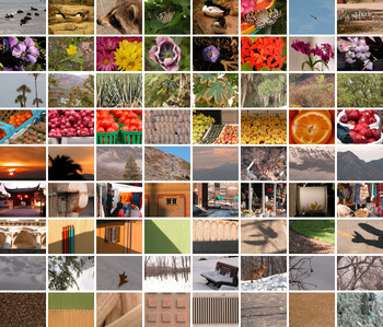
The McGill calibrated color image database contains 708 images (Olmos & Kingdom, Reference Olmos and Kingdom2004a). The images have a size of 768 × 576 pixels and are grouped into nine categories, namely animals, flowers, foliage, fruits, land and water, man-made, shadows, snow, and textures (Fig. 1). The images are stored as standard RGB images in TIFF and were converted to LMS cone excitation space using a conversion function provided by the authors of the database.
(Color online) Sample images of each category of the McGill database. Each row shows sample images from the nine categories of the image database (animals, flowers, foliage, fruits, land and water, man-made, shadows, snow, and textures).

The calibration procedure used to generate the conversion function was developed by T. Troscianko and A. Parraga (University of Bristol, UK) and has been described elsewhere (Párraga et al., Reference Párraga, Troscianko and Tolhurst2002; Johnson et al., Reference Johnson, Kingdom and Baker2005). Briefly, the calibration involves a gamma-correction and a measurement of the spectral sensitivities of the RGB camera sensors. For the gamma correction, the luminance response functions of the camera RGB sensors were determined by illuminating a set of six gray Munsell papers and taking average RGB camera values as well as measured luminance values. A gamma function was then fitted and inverted to linearize the mapping between RGB values signaled by the camera and measured luminance values. The spectral sensitivities of the three camera sensors were measured by taking photographs of a white target through a series of optical narrow-band interference filters spanning the range from 400 to 700 nm. The calibration process converts an RGB camera image to a trichromatic representation, where each pixel contains the relative capture ratios of the three human cones L, M, and S based on the Smith and Pokorny (Reference Smith and Pokorny1975) cone fundamentals.
Unlike hyperspectral images, this method is limited by the gamut of the camera: highly saturated colors outside the gamut would generate the same sensor response and cannot be distinguished. Another problem is that wavelengths that are metameric for the camera are not metameric for the LMS cones if the camera RGB sensitivities are not a linear transformation of the cone sensitivities.
A subset of the images contained a pixel fault of the camera, resulting in a small region of bright-green pixels. Those images were identified by visual inspection and then cropped to the largest rectangle that did not contain the faulty pixels.
Computation of color-opponent responses
The calibrated images were first transformed into LMS cone space, modeling responses of the L, M, and S cones of a human observer. Next, LMS responses were transformed into a color-opponent space of a luminance signal (Lum) and two chromatic signals [L − M and S − (L + M)], resembling the chromatic preferences of retinal ganglion cells and cells in the lateral geniculate nucleus (LGN). Formally, the following transformations of the LMS cone excitations were used (Párraga et al., Reference Párraga, Troscianko and Tolhurst2002; Johnson et al., Reference Johnson, Kingdom and Baker2005):



The parameter ε = 2−52 is a small constant, which is added to avoid division by zero in the computation of LM and SmLM.
The resulting chromatic cone-opponent responses were normalized to unity across channels by the global maximum of each channel: each LM image was divided by the maximum value across all LM images, and each SmLM image was likewise divided by the maximum value across all SmLM images. The luminance images were each individually normalized to unity. This different treatment was necessary because of the large variation in luminance (over several orders of magnitude) with few images of extremely high luminance values. On the one hand, globally normalizing also the luminance images would have mapped the luminance values of most images to a small fraction of the full range. On the other hand, locally normalizing also the chromatic images would have artificially generated maximum chromatic contrast in each image. The present choice thus ensures that the chromatic edge contrast is not due to an artificial local normalization of the responses in the chromatic channels. As a side effect, the luminance images have a larger contrast.
In a control evaluation, we also employed a linear conversion:



These equations are similar to the orthonormal principle axes found by Ruderman et al. (Reference Ruderman, Cronin and Chiao1998); they only differ in excluding S in the computation of Lum and omitting a scalar scaling that has been used by Ruderman et al. (Reference Ruderman, Cronin and Chiao1998) to normalize the axes to unity.
Gaussian blurring, edge detection and joint histogram computation
After the global normalization of the chromatic planes and the local normalization of the luminance plane, the resulting maps were convolved with a Gaussian filter with a small standard deviation of σ = 1 pixel to reduce noise in the images. In some cases, a larger standard deviation of σ = 16 was used to analyze the edge responses on a larger scale.
Next, edges were detected in the three color-opponent planes using the Sobel operator. The Sobel operator is a 3 × 3 filter that realizes an approximation of the first derivative by central differences Dx combined with a blurring along the edges by a binomial filter B. The Sobel filter is defined as:

Edges were determined in horizontal and vertical directions, and the resulting responses were averaged to obtain a polarity-sensitive estimation of edge contrast for each location in the image:

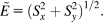
In a control evaluation, we also used the gradient magnitude as an estimation of the polarity-insensitive edge energy:
Finally, a joint histogram of edge strengths was computed to characterize the co-occurrence of edges in the different color-opponent planes. In a joint histogram, the value at position (i, j) is the number of pixels with value i in one channel and value j at the same location in the other channel. The joint histogram is an approximation of the joint probability density of pairs of edge pixels at same locations in different color channels. For each image, three joint histograms of edge contrasts were computed for each combination of the two edge images (Lum/LM, Lum/SmLM, and LM/SmLM). Histograms were averaged across images to obtain the final joint histograms of the three edge combinations. Because most pixels in an image are not an edge, the joint edge histograms peak at zero contrast. The joint histogram images shown in the Results section are log-transformed for display purposes.
Mutual information
The mutual information of two discrete random variables X and Y is defined as:

where p(x, y) is the joint probability distribution function of X and Y and p 1(x) and p 2(y) are the marginal probability distribution functions of X and Y, respectively (Shannon, Reference Shannon1948; Deco & Obradovic, Reference Deco and Obradovic1997). Mutual information is measured in bits and gives the amount of information that X and Y share. Mutual information is zero for independent random variables. Mutual information is maximal if the random variables are dependent. The maximum value that the mutual information can assume depends on the number of discrete elements in the random variables: If the random variables X and Y both have N discrete elements, the maximum mutual information between X and Y is log2(N). Thus, for edge histograms of N × N bins, the mutual information can take a maximum value of log2(N); for example, 10 for N = 1024 bins. Unless noted otherwise, all reported values of mutual information are for bin size 1024.
Results
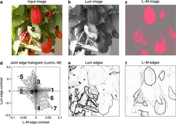
Starting with a separation of the image in a luminance plane and two chromatic planes, we computed the joint edge histogram that reveals the co-occurrence of chromatic and luminance edge contrasts. Results for a sample image and the joint statistics of luminance and L − M edges are shown in Fig. 2.
(Color online) Overview of the joint histogram computation. A color image (a) is separated into a luminance image (b) and an L − M image (c) (signaling reddish-greenish variations), and edges are detected in each image (e, f). From the edge images, a joint edge histogram (d) is computed. The different shades of gray in the joint histogram code the different frequencies of co-occurrence of the edge contrasts: The darker, the more frequent. The joint edge histogram peaks at zero contrast, because most pixels in an image are not an edge. More interestingly, the edge strengths in the two planes are largely independent: purely chromatic edges (1, 2, 8) occur as well as purely luminance edges (3, 4) or edges that combine chromatic and luminance contrasts (5, 6, 7). A contrast in one dimension is not predictive for the most likely contrast in the other dimension.

In a joint edge histogram, the value at the position (i, j) denotes the number of pixels with edge contrast i in one channel and edge contrast j at the same location in the other channel. The darker the gray, the more frequent is the particular combination of edges. The joint edge histogram in Fig. 2 peaked at zero contrast, because edges are rare events and most pixels in an image are not an edge. This was a general pattern that occurred in all images. More interesting are the points in the joint histogram that correspond to nonzero contrast in one or two channels. For this image, we have strong responses along the achromatic luminance axis (sample points 3 and 4 in Fig. 2) and also along the L − M axis (sample points 1 and 2). Points in the joint histogram along the chromatic L − M correspond to isoluminant edges, which were obviously present in this image, and also in the joint histogram of all images of the database, as will be shown below. There were also edges that combined chromatic and luminance contrasts (e.g., sample points 5, 6, and 7). These points fell along the second diagonal, where a red–green contrast co-occurs with a dark–light contrast. The reverse combination of contrasts (bright red next to dark green) was less frequent, resulting in few gray values of high joint contrast along the main diagonal in the joint histogram.
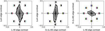
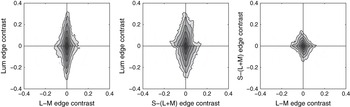
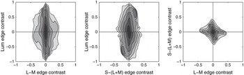
To investigate the global pattern of the co-occurrence of chromatic and luminance edges, we computed the joint edge histograms for all 708 images of the McGill database (Olmos & Kingdom, Reference Olmos and Kingdom2004a). For each image, three joint edge histograms were computed for the possible combinations of edges detected in the three channels, a luminance channel (Lum) and two chromatic channels [L − M and S − (L + M)]. The two chromatic channels were derived by combining input from the three types of cones (L, M, and S) in an opponent way. The joint edge histograms averaged across images are depicted in Fig. 3. We found that isoluminant edges exist in natural scenes and were not rarer than pure luminance edges. Most edges combined luminance and chromatic information, but to varying degrees such that a contrast in one dimension was not predictive for the most likely contrast in the other dimension.
(Color online) Joint edge histograms for the McGill color calibrated image database. Joint histogram of the edges in the luminance channel and the L − M channel (left), the luminance channel and the S − (L + M) channel (middle), and edges in the two chromatic channels [L + M and S − (L − M), right].

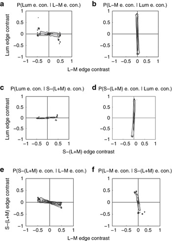
We found that edges in the three dimensions were statistically independent. We quantified the statistical independence by a measure of mutual information between the edges signaled in the two channels. The mutual information between any two channels was small [Lum/L − M: 0.071 bits, Lum/S − (L + M): 0.078 bits, and L − M/S − (L + M): 0.21 bits, for bin size 1024]. Examining the conditional probabilities confirmed the independence (Fig. 4): for example, all luminance edge contrasts were approximately equally probable given a L − M edge contrast (Fig. 4a), and all L − M edge contrasts were approximately equally probable given a luminance contrast (Fig. 4b). A contrast in one dimension was not predictive for the most likely contrast in the other dimension. Based on these data, we conclude that there is a substantial degree of independence between chromatic and luminance edges in natural scenes.
Conditional probabilities of joint edge contrasts in natural scenes. (a) Conditional probability of observing a certain luminance edge contrast given a specified L − M edge contrast. The conditional probability is obtained by normalizing vertical slices of the L − M/Lum edge histogram shown in Fig. 3. The darker the gray level, the higher the conditional probability. (b) Conditional probability of observing a certain L − M edge contrast given a specified luminance edge contrast. The conditional probability is obtained by normalizing horizontal slices of the L − M/Lum edge histogram shown in Fig. 3. (c, d) Conditional probabilities of for the S − (L + M)/Lum edge histogram, format as in a, b. (e, f) Conditional probabilities of for the L − M/S − (L + M) edge histogram, format as in a, b. e. con., edge contrast.

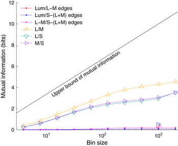
The maximum mutual information depends on the bin size: For histograms of N bins, the maximum mutual information is log2(N), for example, 10 for 1024 bins. The choice of bin size may be critical, as using too many bins leads to a noisy estimate and too few bins to an oversmoothed estimate. To investigate how sensitive the mutual information is to the choice of bin size, we computed mutual information for bin sizes from 4 to 2048 in 10 logarithmic steps (Fig. 5). A closer inspection of the mutual information for the joint edge histograms revealed that the mutual information saturates for bin sizes above about 512; values of the mutual information for bin sizes of 512 and above are thus stable estimates. To provide an intuition about how big or small the mutual information of the joint edge histograms is, we also computed mutual information between cone responses that are known to be highly correlated (Buchsbaum & Gottschalk, Reference Buchsbaum and Gottschalk1983; Ruderman et al., Reference Ruderman, Cronin and Chiao1998). The mutual information between the L and M cones was 4.30 bits, between the L and S cones 2.97 bits, and between the M and S cones 2.05 bits (for bin size 1024). These values were an order of magnitude above the values obtained for the joint edge histograms.
(Color online) Dependence of mutual information on bin size. Mutual information for the joint edge histograms saturates for bin sizes above 512 and is an order of magnitude smaller than the mutual information between cone responses. Mutual information remains small if cone-opponent channels were not normalized by the responses of L and M cones (open circles at bin size 1024), also if a polarity-insensitive computation of edge strength was used (crosses at bin size 1024; crosses and open circles have been slightly displaced to increase visibility).

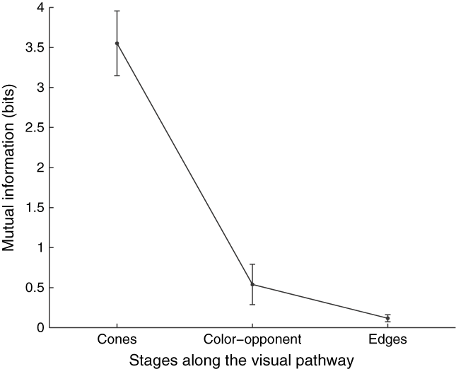
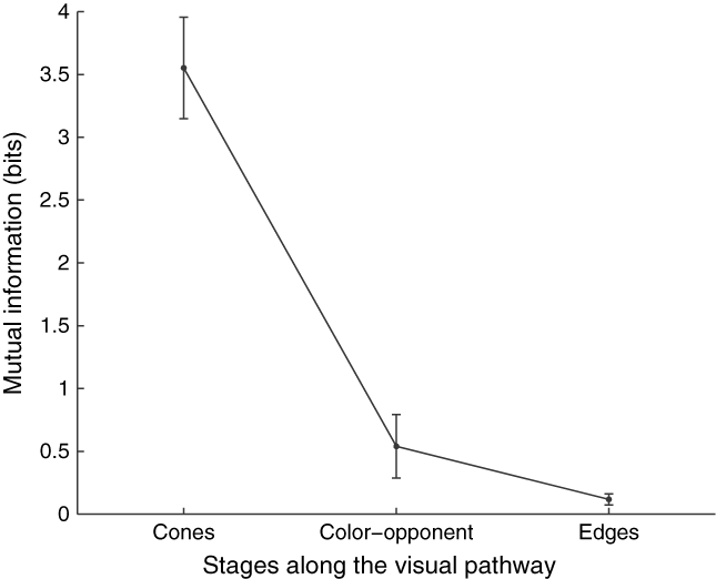
The efficient coding hypothesis states that the visual system strives for independence; various anatomical or physiological constraints of the neural processing may prevent that independence is achieved. Instead, it has been proposed that successive stages of processing along the ascending sensory pathway should reduce statistical dependence (Simoncelli, Reference Simoncelli2003). Confirming this hypothesis, Chechik et al. (Reference Chechik, Globerson, Tishby, Anderson, Young, Nelken, Dietterich, Becker and Ghahramani2002) demonstrated experimentally that mutual information is reduced along the cat auditory pathway. Here we investigated whether a reduction in mutual information also occurs along the visual pathway, from cones via precortical postreceptoral channels (eqns. 4–6) to cortical edge-sensitive neurons modeled by a standard edge detector (eqn. 7). We found that mutual information was reduced along the model visual pathway (Fig. 6). The largest reduction in redundancy occurs at the second stage, where the highly correlated cone responses are decorrelated and become largely independent in the color-opponent channels. Mutual information was then further reduced at the cortical stage of edge-sensitive neurons. At the cortical stage, also the differences in mutual information between the different channels were equalized, resulting in a smaller standard error.
Reduction of mutual information as one ascends the visual pathway. Mutual information decreases during visual processing; the information represented in the different channels becomes more independent. Furthermore, the mutual information in the three channels at the successive stages is equalized [stage 1: L, M, S cones, stage 2: L − M, S − (L + M), Lum color-opponent channels, and stage 3: edges in the three color-opponent channels], as shown by the decreasing error bars (denoting ± 1 s.e.m.).
The mutual information between the edge responses also depends on the equation used to transform the cone responses into color-opponent channels. So far, we have used equations that incorporate a normalization of the chromatic channels by the combined L and M cone responses (eqns. 1–3). If a linear combination of cone responses was used instead (eqns. 4–6), mutual information between channels was slightly larger, namely Lum/L − M: 0.306 bits, Lum/S − (L + M): 0.596 bits, and L − M/S − (L + M): 0.24 bits (open circles in Fig. 5).Footnote 1 If minimizing mutual information between channels is one goal of early visual processing, then these results suggest that the chromatic channels should undergo a nonlinear divisive normalization by the combined responses of L and M cones.
To address the influence of the edge computation on the estimation of mutual information, we also used a polarity-insensitive edge energy operator (eqn. 9) rather than the polarity-sensitive estimation of edge contrast and applied it to a linear combination of cone inputs. The mutual information between edges in the three channels was small [Lum/L − M: 0.419 bits, Lum/S − (L + M): 0.56 bits, and L − M/S − (L + M): 0.39, crosses in Fig. 5] and of the same magnitude as obtained above for the linear combination of cone inputs and the polarity-sensitive estimation of edge contrast.
It has been shown that luminance and chromatic contrast are independent in natural scenes (Mante et al., Reference Mante, Frazor, Bonin, Geisler and Carandini2005). Here we found that edge contrasts in the luminance channel and in the chromatic channels are also independent of each other and provide independent sources of information. The independence of edge contrasts has an important implication: for independent cues, a linear model is optimal (Jacobs, Reference Jacobs1995). Linear models allow the integration of new cues that can be simply added to the existing system when they become available (Zhou & Mel, Reference Zhou and Mel2008).
The independence was not perfect, in particular between the edges detected in the two chromatic channels, as indicated by the small but nonzero mutual information. The mutual information between edges in the two chromatic channels was about twice as large as that between luminance and chromatic edges. This was reflected by a larger negative correlation between the edges in the two chromatic channels (−0.36 ± 0.01), in accordance with previous findings (Webster & Mollon, Reference Webster and Mollon1997), and also visible as a slightly larger elongation along the second diagonal in the joint histogram for the chromatic L − M and S − (L + M) edges (Fig. 3). This direction corresponds to edges between yellow and blue objects, such as rock or dry leaves against blue sky. The within-image correlation between luminance and L − M edges was small (−0.12 ± 0.01), as well as between luminance and S − (L + M) edges (0.17 ± 0.01).
The shapes of the joint histograms that combine luminance and chromatic edges are also not perfectly symmetric and ellipsoidal but slightly slanted and diamond-shaped. The Lum/L − M and Lum/S − (L + M) edge histograms have higher excursions for bright-green contrasts that could be attributed to the luminous efficiency function that peaks in the greenish part of the spectrum. The Lum/L − M joint edge histogram tapered along the L − M axis, due to higher contrast in this direction. This pattern occurred for images of another database, was not an artifact of the analysis along cardinal directions, and did not occur for contrast measured between random locations (Appendix). The data suggest that chromatic contrast is particularly high in the direction sensed by the third chromatic system in the evolution, the L − M system.
The joint histograms were elongated along the luminance axis. The edge contrast along the luminance axis was about twice the contrast along the chromatic axes, mainly due to the different methods of scaling the channels. More importantly, a considerable fraction of all edges, namely all edges in the horizontal segment between the main and the second diagonal in the joint edge histograms, had a higher contrast along the chromatic axis than along the luminance axis and could thus be detected better by the chromatic system. Furthermore, the widths of the different shades of gray areas in the joint histograms were approximately equal along the luminance and the chromatic axes: there were as many pure luminance edges as there were pure chromatic edges in natural scenes. If purely chromatic, that is, isoluminant, edges would be rarer than chromatic edges, the joint histograms would contract along the chromatic axes. This was not the case: in natural scenes, isoluminant edges are as frequent as pure luminance edges.
Analysis of categories
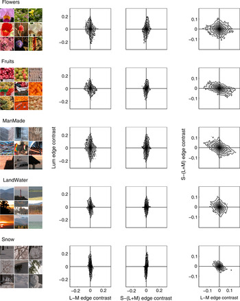
In the analysis done so far, we pooled images from all categories in the database (animals, flowers, foliage, fruits, land and water, man-made, shadows, snow, and textures). One might expect that the joint histograms differ for the different categories: High-contrast chromatic edges are more likely to occur in colorful images (such as flowers and fruit) and less likely in basically achromatic images such as those depicting snow. We tested this hypothesis by computing the joint histograms separately for each category. Examples for four representative categories are shown in Fig. 7. The joint histograms showed the expected pattern. Joint histograms for categories such as flowers and fruit with colorful images had larger excursions along the chromatic axes. Likewise, joint histograms for categories such as snow and landscape had only small excursions along the chromatic axes. Interestingly, man-made scenes also had many high-contrast chromatic edges, leading to larger excursions along the chromatic axes. It has been shown that color facilitates object recognition and allows one to memorize objects better (Wichmann et al., Reference Wichmann, Sharpe and Gegenfurtner2002) and to recognize them faster (Gegenfurtner & Rieger, Reference Gegenfurtner and Rieger2000). The high-contrast chromatic edges in man-made scenes may then reflect that humans colorize their world to take advantages of these benefits.
(Color online) Joint edge histograms for different categories of the McGill color image database.

Influence of scale
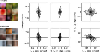
The spatial sensitivity for color and luminance differs. The luminance channel (L + M) responds better to fine spatial detail than the postreceptoral color channels L − M and S − (L + M) (Kelly, Reference Kelly1983; Mullen, Reference Mullen1985; Poirson & Wandell, Reference Poirson and Wandell1993, Reference Poirson and Wandell1996). Here we investigated whether the differences in sensitivity of the human visual system are reflected somehow in the distribution of chromatic edges in natural scenes. If the low-pass sensitivity of the human chromatic system would be reflected in the spatiochromatic characteristics of natural scenes, blurring should increase the relative strengths of chromatic versus luminance edges. Blurring removes the high-frequency components in the image. If color in natural scenes would be of a coarser scale, blurring should affect the luminance channel more than the chromatic channels. As a consequence, the shape of the joint histogram for the blurred images should be different from the shape of the joint histogram of the unblurred images: Instead of being elongated along the luminance axis, the joint edge histograms on a coarser scale should be elongated along the chromatic axes. To investigate the edge responses on a coarser scale, we blurred the images considerably with a Gaussian (σ = 16 pixels) and computed the joint edge histograms (Fig. 8). Gaussian blurring is the standard operation in image processing to derive images at different spatial scales (Lindeberg, Reference Lindeberg1994). Because blurring reduces the overall contrast, the magnitude of the edge responses for all dimensions was reduced by a factor of about 1/10 (compare scale in Figs. 7 and 8). However, the overall pattern did not change. Luminance edges remained of stronger contrast, and we did not find that chromatic edges in natural scenes were stronger at lower spatial frequencies.
(Color online) Joint edge histograms for large-scale edges of the McGill color image database. The blurring reduces the contrast, but the overall shape of the joint edge histograms is the same as for the unblurred images (Fig. 7). Results are shown for two categories with lots of colors (Flowers and ManMade). Histograms obtained for the other categories were also similar to those obtained for the unblurred images.

The mutual information between the luminance channel and the chromatic channels was small and of similar magnitude as for the unblurred versions [Lum/L − M: 0.030 bits and Lum/S − (L + M): 0.043 bits]; the mutual information between the two chromatic channels was about twice the value obtained for the unblurred images [L − M/S − (L + M): 0.178 bits].
Overall, the low sensitivity of the human visual system to chromatic variations of high spatial frequency seemed not to be matched to the statistics of natural scenes. This finding is in accordance with other studies showing that the preference of the chromatic system for low spatial frequency is not reflected in any differences between luminance or chromatic amplitude spectra in general natural scenes (Webster & Mollon, Reference Webster and Mollon1997; Párraga et al., Reference Párraga, Brelstaff, Troscianko and Moorehead1998). A slightly steeper slope in the amplitude spectra of the L − M channel has only been reported for special scenes such as red fruit among green leaves (Párraga et al., Reference Párraga, Troscianko and Tolhurst2002). It has been hypothesized that the computations in the brain aim at a reduction of the redundancy present in the visual input and that the properties of the visual system can be inferred from the statistics of natural scenes (Barlow, Reference Barlow and Rosenblith1961); the low spatial resolution of the chromatic system should be paralleled by a lower resolution of chromatic information in natural scenes. Here we find no differences in the joint histograms computed on different scales. Instead, we find that the observed independence of luminance and chromatic edges is stable across scale variations.
Discussion
Summary of findings
We analyzed the co-occurrence of color and luminance edges in natural scenes. We found that edges in the luminance channel and in the two chromatic channels L − M and S − (L + M) were independent. Independence increased along successive stages of visual processing, from cones via color-opponent channels to edges. The largest increase occurred at the first step, where cone responses are transformed into color-opponent channels. We also analyzed the joint statistics on a coarser scale where we found basically the same independence of luminance and chromatic edges.
Comparison to previous studies
Previous studies of the joint distribution of color and luminance were based on synthetic stimuli (Buchsbaum & Gottschalk, Reference Buchsbaum and Gottschalk1983), few (12–29) natural images (Ruderman et al., Reference Ruderman, Cronin and Chiao1998; Wachtler et al., Reference Wachtler, Lee and Sejnowski2001; Fine et al., Reference Fine, MacLeod and Boynton2003), or used uncalibrated JPEG images (Heidemann, Reference Heidemann2006; Zhou & Mel, Reference Zhou and Mel2008). Only a single study investigated the joint statistics of differences between the achromatic and chromatic signals (Fine et al., Reference Fine, MacLeod and Boynton2003).
Early investigations into the distribution of colors in natural scenes have focused on the efficient coding of the highly correlated cone responses in the subsequent processing. Buchsbaum and Gottschalk (Reference Buchsbaum and Gottschalk1983) investigated how the highly correlated cone responses could be efficiently coded for optimal color information transmission in the retina. They found that the cone signals can be decorrelated by an orthogonal linear transformation resembling a luminance-like channel and two chromatic opponent channels. The derivation of this transformation was dependent solely on criteria from information theory and was confirmed for natural images (Ruderman et al., Reference Ruderman, Cronin and Chiao1998).
The study by Buchsbaum and Gottschalk (Reference Buchsbaum and Gottschalk1983) gave insight into the decorrelation of cone responses in the color-opponent channels without considering the spatial structure of the signals. A principal components analysis (PCA) of the spatiochromatic structure revealed that the luminance and chromatic dimensions of the second-stage channels were entirely decorrelated, that is, based on activity in one channel, one cannot linearly predict the activity in another channel (van Hateren, Reference van Hateren1993; Webster & Mollon, Reference Webster and Mollon1997; Ruderman et al., Reference Ruderman, Cronin and Chiao1998). Ruderman et al. (Reference Ruderman, Cronin and Chiao1998) further noted that the activities are uncorrelated but not independent. For example, large changes in all three dimensions occur at object boundaries.
These studies computed PCAs for small patch sizes (3 × 3 or 7 × 7 pixels). Wachtler et al. (Reference Wachtler, Lee and Sejnowski2001) also employed an independent component analysis (ICA) and found basis functions with pronounced opponency that did not always coincide with the color space axes. In particular, red–green basis functions were tilted with respect to the L − M cone axis, signaling orange-bluish variations, which may reflect the negative correlation of L − M and S cone–opponent signals in natural images (Webster & Mollon, Reference Webster and Mollon1997). We also find an elongation along the second diagonal in the L − M/S − (L + M) joint edge histogram (Fig. 3).
Heidemann (Reference Heidemann2006) determined the principal components of natural images for larger patch sizes (128 × 128 pixels) and found basis functions that were all spatially structured, showing that the physical structure of a scene is expressed both in color and in luminance. In other words, the same spatiochromatic structure of edge, bar, and grating patterns emerged both in color and in luminance.
The work reviewed so far has analyzed the spatiochromatic structure of natural scenes but not the joint statistics of differences in these dimensions. As noted above, the activities in the postreceptoral channels have been found to be uncorrelated but not independent:Footnote 2 differences in luminance between two pixels may very well be associated with differences in chromaticities. One may have the intuition that two pixels that fall on different surfaces are likely to differ both in luminance and in color. Based on an analysis of the 12 hyperspectral images recorded by Ruderman et al. (Reference Ruderman, Cronin and Chiao1998), this seems to be confirmed: for pixels of a given separation, the sign and magnitude of the changes are uncorrelated, but differences in luminance and color were found to be not fully independent (Fine et al., Reference Fine, MacLeod and Boynton2003).
Here we computed joint probability density functions similar to Fine et al. (Reference Fine, MacLeod and Boynton2003) for a large number of calibrated color images (708 images from the McGill database). Contour plots of the joint edge histograms (i.e., the joint probability density functions multiplied by a constant scalar) did not show higher values along the diagonals compared to the main axes, as would be the case if the channels were not independent. We found no such structure in any of the averaged joint histograms. A difference in luminance may coincide with a difference in chromaticity, or may not, with equal probability. These results parallel the finding that luminance and contrast are independent in natural scenes (Mante et al., Reference Mante, Frazor, Bonin, Geisler and Carandini2005). We have shown that isoluminant edges are as likely as purely achromatic edges or any other edge combining chromatic and achromatic differences at a fixed ratio.
The (wrong) intuition that chromatic and luminance edges are dependent may have its origin in simplistic scenes of homogeneous objects viewed against homogeneous backgrounds, where a luminance contrast occurs together with a chromatic contrast. In natural scenes, however, objects are rarely of homogeneous color, backgrounds are variegated, and shadows cast luminance boundaries all over the scene.
Relation to physiological findings and imaging studies
In physiology, it was long thought that luminance information was used only for the processing of edge information, whereas cells responsive to color would exhibit no orientation tuning at all (Livingstone & Hubel, Reference Livingstone and Hubel1984). However, work by Thorell et al. (Reference Thorell, De Valois and Albrecht1984) that was later confirmed and extended by Johnson et al. (Reference Johnson, Hawken and Shapley2001, Reference Johnson, Hawken and Shapley2008) found a large number of neurons in primary visual cortex that do respond to color and luminance stimuli with a similar spatial tuning. Other investigators have shown that tuning to color and orientation is independent in both primary and secondary visual cortex (Gegenfurtner et al., Reference Gegenfurtner, Kiper and Fenstemaker1996; Friedman et al., Reference Friedman, Zhou and von der Heydt2003). When color and orientation selectivity are determined by indices corresponding to the degree of selectivity of the tuning for each neuron, the two indices are uncorrelated. This independence of the tuning properties of the population of neurons corresponds quite well with the independence of these properties in the natural environment.
Chromatic contrast is also signaled by double-opponent cells that lack circular symmetry and have an orientation bias. Double-opponent cells have spatially opponent and cone-opponent receptive fields that are wired-up to encode spatial aspects of the world and have been shown to respond to color edges (Conway, Reference Conway2001; Conway & Livingstone, Reference Conway and Livingstone2006).
Recently, it has been shown using high-field BOLD functional magnetic resonance imaging in combination with a multivariate data analysis that signals recorded in V1, V2, and V3 could directly discriminate between orientations based on chromatic information (Sumner et al., Reference Sumner, Anderson, Sylvester, Haynes and Rees2008). These results are in accordance with the properties of neurons in the early visual areas that are selective for a combination of orientation and chromatic information. Interestingly, and in accordance with our findings, a combined processing was found not only for luminance and L − M but also for the S cone signals, which are conveyed to the cortex via a separate koniocellular channel (Dacey, Reference Dacey2000; Chatterjee & Callaway, Reference Chatterjee and Callaway2003).
Combination of chromatic and luminance information
One basic task in vision is to detect objects. Objects differ from their background in any or all dimensions of color, brightness, texture, disparity, movement, and so on. The reliability of these cues varies, and the visual system can often rely on many of them. One circumstance in which color can segment objects from their background is when there are accidental variations in brightness caused by cast shadows (Lennie, Reference Lennie, Gegenfurtner and Sharpe1999; Kingdom, Reference Kingdom2003; Kingdom et al., Reference Kingdom, Beauce and Hunter2004). One important question is, when is information from different cues combined?
Unoriented luminance contrast and chromatic information is combined already in the retina by parvocellular ganglion cells (De Valois & De Valois, Reference De Valois and De Valois1988). Oriented chromatic and luminance contrast is processed at the next cortical stage, at the level of V1 orientation-selective color–luminance cells (Johnson et al., Reference Johnson, Hawken and Shapley2001, Reference Johnson, Hawken and Shapley2004, Reference Johnson, Hawken and Shapley2008). These cells can integrate information of the different independent channels to signal object boundaries. However, our finding of the independence of color and luminance edges in natural scenes is also compatible with the alternative view that this independence drove the evolution of independent cortical processing streams for color form and luminance form because the two cues provide different pieces of information about the natural world. The independence may also explain why the visual system evolved two independent precortical pathways for processing chromatic information, the parvocellular and koniocellular pathways.
The critical question that would get at the heart of this issue is whether the cues associated with color edges are qualitatively different from those associated with luminance edges; that is, is there a special value of color edges in distinguishing and recognizing objects? Studies showing that color allows one to memorize objects better (Wichmann et al., Reference Wichmann, Sharpe and Gegenfurtner2002) and to recognize them faster (Gegenfurtner & Rieger, Reference Gegenfurtner and Rieger2000) could be interpreted as showing that color provides access to a different kind of information about the world than is provided by luminance form.
These ideas may be reconciled by multiple cortical streams, one were color and luminance are combined early to signal object boundaries, and another were cone-opponent neurons signal chromatic surface properties (Conway, Reference Conway2001; Conway et al., Reference Conway, Hubel and Livingstone2002). Both streams could be involved in the computation of perceived surface color. Filling-in processes are potential candidates for this integration (Grossberg, Reference Grossberg1987, Reference Grossberg2000; Neumann et al., Reference Neumann, Pessoa and Hansen2001).
Relation to psychophysical findings
The spatial resolution of chromatic information is poor compared to the luminance system. Contrast sensitivity for gratings above 0.5 cycles/deg is higher for luminance than for chromatic gratings (Kelly, Reference Kelly1983; Mullen, Reference Mullen1985; Sekiguchi et al., Reference Sekiguchi, Williams and Brainard1993). The spatial contrast sensitivity has a low-pass tuning curve for chromatic contrast and a band-pass tuning curve for achromatic contrast. It has been hypothesized in a seminal article by Barlow (Reference Barlow and Rosenblith1961) that the computations in the brain aim at a reduction of the redundancy present in the visual input and that the properties of the visual system can be inferred from the statistics of natural scenes (for reviews, see Simoncelli & Olshausen, Reference Simoncelli and Olshausen2001; Geisler, Reference Geisler2008). Taken together, the low spatial resolution of the chromatic system should be paralleled by a lower resolution of chromatic information in natural scenes. Such a link has been found by investigating the slope of the spatial frequency spectrum (Párraga et al., Reference Párraga, Troscianko and Tolhurst2002) but only for special—and likewise ecologically relevant—scenes of fruits among leaves. Previous studies have found no such link for general natural scenes by investigating the slope of the spatial frequency spectrum, that is based on the computation of spatial content globally across the whole image (Webster & Mollon, Reference Webster and Mollon1997; Párraga et al., Reference Párraga, Brelstaff, Troscianko and Moorehead1998). Here we investigated the local contrast and found that the joint statistic between chromatic and luminance edges did not differ between coarse and fine scales. This finding is in accordance with previous global statistics but shows that the visual system seems not always to be able to adapted to the statistics of natural scenes. One possible explanation is that the adaptation of the visual system is constrained by several other factors, such as the two-dimensional layout of the retina, that prevents each type of cone photoreceptor being present at each location.
Besides the differences in the tuning characteristic of the spatial contrast sensitivities, the processing of achromatic and chromatic forms is highly similar (Shevell & Kingdom, Reference Shevell and Kingdom2008). Contrast sensitivity in luminance and color vision is based on the processing in different spatial frequency channels, with similar tuning widths for chromatic and achromatic processing (Bradley et al., Reference Bradley, Switkes and Valois1988; Switkes et al., Reference Switkes, Bradley and Valois1988; Webster et al., Reference Webster, De Valois and Switkes1990; Losada & Mullen, Reference Losada and Mullen1995; Reisbeck & Gegenfurtner, Reference Reisbeck and Gegenfurtner1998). Chromatic and achromatic processing is also highly similar at subsequent processing where local orientations are grouped into coherent contours (McIlhagga & Mullen, Reference McIlhagga and Mullen1996; Mullen et al., Reference Mullen, Beaudot and McIlhagga2000) and contour shapes are extracted (Mullen & Beaudot, Reference Mullen and Beaudot2002; Gheorghiu & Kingdom, Reference Gheorghiu and Kingdom2007). Furthermore, the tilt illusion that depends on the interaction between orientation-specific channels also exists for isoluminant stimuli (Clifford et al., Reference Clifford, Spehar, Solomon, Martin and Zaidi2003), and the strengths of various geometric–optical illusions are the same for achromatic and isoluminant stimuli (Hamburger et al., Reference Hamburger, Hansen and Gegenfurtner2007).
Edge detection algorithms
In computer vision, edge detection algorithms were mostly designed for the processing of achromatic images. However, despite tremendous effort, the multipurpose edge detector that faithfully detects the relevant edges in an image has not been found yet. This failure may point to the importance of other visual modalities apart from luminance that play an important role in edge detection. Only comparably few attempts have been made to implement a chromatic edge detection algorithm (e.g., Nevatia, Reference Nevatia1977; Delcroix & Abidi, Reference Delcroix, Abidi and Hsing1988; Lee, Reference Lee1990).
Based on the notion that color can be used to separate reflection components, a dichromatic reflection model has been proposed (Shafer, Reference Shafer1985). The dichromatic reflection model is a method for analyzing a standard color image to determine intrinsic images of the specular and diffuse reflection at each pixel. This model provided the basis for algorithms for color-based object recognition that are invariant against shadows and specularities (Klinker & Shafer, Reference Klinker and Shafer1990; Gevers & Smeulders, Reference Gevers and Smeulders2000). van de Weijer et al. (Reference van de Weijer, Gevers and Smeulders2006) combined the dichromatic model with a structure tensor approach to compute robust photometric invariant features.
Other studies have investigated the optimal combination of achromatic and chromatic cues to maximize the reliability of object boundary detection (Martin et al., Reference Martin, Fowlkes and Malik2004; Zhou & Mel, Reference Zhou and Mel2008). It has been found that a linear model suffices for optimal cue combination (Martin et al., Reference Martin, Fowlkes and Malik2004). A linear model allows the easy incorporation of additional cues when they become available (Zhou & Mel, Reference Zhou and Mel2008) but is optimal only if the cues are independent (Jacobs, Reference Jacobs1995). Edge responses at neighboring locations can show strong statistical dependencies (Schwartz & Simoncelli, Reference Schwartz and Simoncelli2001; Zetzsche & Röhrbein, Reference Zetzsche and Röhrbein2001), and differences in chromatic and luminance channels have been found to be not entirely decorrelated (Fine et al., Reference Fine, MacLeod and Boynton2003). However, the study by Fine et al. (Reference Fine, MacLeod and Boynton2003) was based on the analysis of only 12 images. Zhou and Mel (Reference Zhou and Mel2008) have argued that the edge responses cannot be independent because the appearance or disappearance of physical edges within overlapping receptive fields will induce a dependency and boost responses in all channels simultaneously; the counter example of an isoluminant edge was believed to be rare in natural scenes (Zhou & Mel, Reference Zhou and Mel2008). Here we have shown based on an analysis of over 700 calibrated images that isoluminant edges are not rarer than purely luminance edges and that the edge responses in any of the three postreceptoral channels are independent. The important implication of the independence is that a simple linear cue combination scheme is sufficient.
Summary
We have analyzed the distribution of chromatic and luminance edges in natural scenes. Isoluminance edges exist in natural scenes and were not rarer than pure luminance edges. Most edges combined luminance and chromatic information, but to varying degrees. We found that chromatic and achromatic edges were statistically independent: the strength of a chromatic edge could not be inferred from the strength of the luminance edge at the same position. Chromatic edges thus provide an independent source of information. Because the edge information is independent, a linear model is optimal for the combination of cues.
It has been shown that color is useful in many different tasks: Color is important in detecting ripe fruit and edible reddish leaves among greenish foliage (Sumner & Mollon, Reference Sumner and Mollon2000a,Reference Sumner and Mollonb), and color helps to detect objects faster (Gegenfurtner & Rieger, Reference Gegenfurtner and Rieger2000) and to memorize them better (Wichmann et al., Reference Wichmann, Sharpe and Gegenfurtner2002). Here we have shown that chromatic information is an independent source of information in natural scenes; color vision allows to access this independent information that then can be used in many different ways.
Acknowledgments
The work was supported by the German Science Foundation (grant Ge-879/5-1). Preliminary results have been reported in abstract form (Hansen & Gegenfurtner, Reference Hansen and Gegenfurtner2007). We are grateful to Bevil R. Conway for many helpful comments and suggestions and to Matthias Bethge, Volker Blanz, Marina Bloj, Rhea T. Eskew, Wilson Geisler, Frederick A. A. Kingdom, P. G. Lovell, Jochem Rieger, Tom Troscianko, Thomas Wachtler, and Christoph R. Witzel for helpful discussion. We also gratefully acknowledge the technical help of Gavin Brelstaff and Thomas Wachtler.
Appendix
We analyzed data from the Bristol hyperspectral images database in addition to the RGB images from the McGill database to ensure that the results are independent of the database and the particular method to estimate cone responses (from either RGB or hyperspectral data). For the Bristol database, we also investigated the origin of the higher contrast along the cardinal axes that appeared in the joint histograms.
Bristol hyperspectral images database
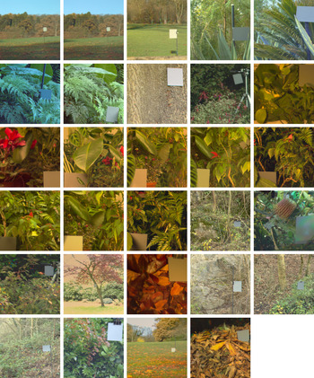
The Bristol hyperspectral images database (Párraga et al., Reference Párraga, Brelstaff, Troscianko and Moorehead1998) consists of 29 images, each comprised 31 spectrally filtered images with a spatial resolution of 256 × 256 pixels. The images show laboratory scenes of plants with different shapes, textures, and colors and images of the British country side and gardens (Fig. 9). The selection of images was aimed at creating a representation of the environment in which primate vision has evolved (Párraga, Reference Párraga1995). The raw images were converted to measured radiance images by a C program. The program has a conversion function for each interference filter that depends on the pixel value, pixel position, filter transmission, lens f-stop, and tube integration time (Párraga et al., Reference Párraga, Brelstaff, Troscianko and Moorehead1998).
(Color online) Rendering of all 29 images of the Bristol hyperspectral images database. The images contain a neutral gray reference card.

LMS cone excitations were obtained from the radiance images by weighting the image spectra with the Stockman and Sharpe (Reference Stockman and Sharpe2000) human cone fundamentals and summing over all wavelengths, that is, by taking the inner product of the image spectra and the cone sensitivities. All subsequent computations were the same as for the McGill image database.
Joint histograms for the Bristol hyperspectral images database
To check whether the results may be biased by the particular choice of the image database, we conducted the analysis on another image database, namely the Bristol hyperspectral images database (Párraga et al., Reference Párraga, Brelstaff, Troscianko and Moorehead1998). The resulting joint histograms are plotted in Fig. 10. The joint histograms were computed for a smaller bin size of 64 because the Bristol database contains fewer images.
Joint edge histograms for the images of the Bristol database.

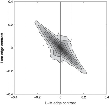
The resulting joint histograms were similar to those obtained for the McGill database, and mutual information between the edges in the different color-opponent channels was small [Lum/L − M: 0.007 bits, Lum/S − (L + M): 0.04 bits, and L − M/S − (L + M): 0.03 bits, for bin size 64]. In particular, the same diamond-shaped structure emerged with particular high activity along the cardinal axes. To further rule out that the increased contrast along the cardinal axes and the resulting deviation from a Gaussian-shaped distribution in the L − M/Lum joint histogram was an artifact of the analysis, we conducted the analysis with the L and M values artificially rotated by 45 deg prior to the subsequent analysis. The resulting joint histogram is depicted in Fig. 11. Any artifact in the analysis would now lead to increasing contrast along the cardinal axes, which would result in a distorted histogram of the rotated L and M values. However, the resulting histogram was basically a rotated copy of the original histogram, ruling out any cardinal bias in the analysis.
Rotated version of the L − M/Lum joint edge histograms for the Bristol database. The high excursions along the diagonals correspond to the high excursions found along the cardinal axes in the unrotated version, showing that these excursions are not an artifact of the analysis rather than a property of the data set.

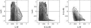
We also computed the joint histograms of the distributions in the three postreceptoral channels Lum, L − M, and S − (L + M) to test whether the joint edge histograms could be already inferred from these more basic channel histograms. The joint histograms of the activity in the postreceptoral channels are plotted in Fig. 12. These joint histograms showed no particular high activity along the cardinal axes. Consequently, the diamond-shaped structure of the edge histograms (Fig. 10) was not already present in the joint distribution of activity within the postreceptoral channels but occurred at the next level, where edge contrast is computed, that is, spatial differences between neighboring activities.
Joint histograms of the postreceptoral channels (before computing the edge responses) for the images of the Bristol database.

To further investigate the origin of the higher contrast along the cardinal axes, we computed histograms on the basis of differences between random locations. This allows us to investigate the effect of the spatial arrangement of chromatic and luminance values in natural scenes.
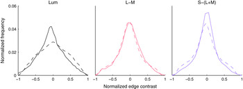
If the higher preferences for the cardinal axes were independent of the spatial arrangement of colors and solely determined by the histogram of the differences between colors at arbitrary locations in the scene, the same diamond-shaped structure as obtained for the edges should also emerge for the random differences. However, we found that this was not the case (Fig. 13). In particular, the Lum/L − M and Lum/S − (L + M) joint histograms obtained from random differences were more rounded and Gaussian-shaped. To quantify the structural dissimilarity, we computed the width:height ratio (averaged across the eight contour levels depicted in Figs. 13 and 10). The joint achromatic–chromatic histograms for the random differences are more elongated [4.2 ± 1.7 s.e.m., vs. 3.4 ± 0.6 for Lum/L − M and 3.5 ± 0.6 vs. 2.6 ± 0.3 for Lum/S − (L + M)], while the joint histograms between the two chromatic channels have almost the same ratio (1.2 ± 0.4 vs. 1.3 ± 0.2). This indicates that in particular the luminance dimension is affected by the random manipulation, resulting in increased luminance contrast. The pattern is also visible from horizontal and vertical cross-sections of the joint histograms (Fig. 14).
Joint histograms of random differences. A joint histogram of random differences is averaged across 1000 different histograms of the database, each obtained with a different realization of the random process for each of the 29 images.

(Color online) Marginal distributions of the joint histograms for contrast edges in natural images (solid) and contrasts between random positions (dashed). The marginal distributions are normalized such that the area under the curve integrates to unity. A pronounced difference between the contrasts between random positions and edges in natural scenes occurs only for the luminance channel.