1 Introduction
The oscillating surface of an acoustically active gas bubble in a liquid becomes unstable as soon as the incident acoustic wave is sufficiently intense. When the driving acoustic pressure exceeds a critical threshold, this instability leads to the onset of shape oscillations corresponding to zonal harmonics of the initially spherical bubble. The mechanism underlying bubble surface oscillations is similar to the Faraday instability creating waves on the surface of a vertically oscillating liquid layer (Benjamin & Ursell Reference Benjamin and Ursell1954). In the specific case of a bubble, the spherical oscillations (the radial or pulsating mode) act as a source for the parametric excitation of shape modes. In recent years, interesting effects of shape oscillations have been reported for coated microbubbles such as armoured bubbles or ultrasound contrast agents used for medical imaging. Dollet et al. (Reference Dollet, van der Meer, Garbin, de Jong, Lohse and Versluis2008) gave evidence that shape modes induce sufficient stress to deform phospholipid monolayers encapsulating the bubble, while Poulichet & Garbin (Reference Poulichet and Garbin2015) and Poulichet, Huerre & Garbin (Reference Poulichet, Huerre and Garbin2017) demonstrated that surface oscillations expel colloidal particles from the bubble surface leading to the desorption of the coating material. Several optical observations of ultrasound-induced bubble fragmentation (Chomas et al. Reference Chomas, Dayton, Allen, Morgan and Ferrara2001; Postema et al. Reference Postema, Van Wamel, Lancée and De Jong2004) also proved that such deformations, when reaching amplitudes comparable to the bubble size itself, can be strong enough to break the shell material and produce several fragments. Finally, microstreaming patterns around bubbles exhibiting surface oscillations show more numerous and localised liquid vortices and higher flow velocities than those induced by classical spherical oscillations (Tho, Manasseh & Ooi Reference Tho, Manasseh and Ooi2007), thus demonstrating their potential interest for liquid mixing at the micro-scale (Ahmed et al. Reference Ahmed, Mao, Juluri and Huang2009) and cell sonoporation (Marmottant, Biben & Hilgenfeldt Reference Marmottant, Biben and Hilgenfeldt2008). Understanding and accurately predicting the above-mentioned effects on the surroundings of the bubble (coating shell material, surrounding liquid, neighbouring objects) requires a proper quantification of the amplitude of the surface oscillations when sustained in the acoustic field.
The most common approach to the dynamics of non-spherical bubbles is to describe the perturbed surface by the equation
 $$\begin{eqnarray}S(r,\unicode[STIX]{x1D703},t)=r-R(t)-\mathop{\sum }_{n=2}^{\infty }a_{n}(t)P_{n}(\cos \unicode[STIX]{x1D703})=0,\end{eqnarray}$$
where
 $r$
and
 $\unicode[STIX]{x1D703}$
are spherical coordinates,
 $R(t)$
is the bubble instantaneous average radius (spherical mode),
 $a_{n}(t)$
are the time-varying amplitudes of the shape modes and
 $P_{n}$
denotes the Legendre polynomial of order
 $n$
. By writing (1.1), we already reduced our analysis to axisymmetric deformations invariant to the third coordinate (
 $\unicode[STIX]{x1D711}$
), thus the spherical harmonics reduce to Legendre polynomials (zonal harmonics). The axisymmetry property is commonly retained in most of theoretical works on non-spherical bubble oscillations and will be considered in the present analysis as well. In addition, some experiments either based on an axisymmetric external forcing (Versluis et al.
Reference Versluis, Goertz, Palanchon, Heitman, van der Meer, Dollet, de Jong and Lohse2010) or a stereoscopic optical set-up (Guédra et al.
Reference Guédra, Cleve, Mauger, Blanc-Benon and Inserra2017) attest to the validity of this assumption.
A further analysis of the non-spherical oscillations is usually conducted for small amplitudes of the deformations by introducing the small parameter
 $\unicode[STIX]{x1D716}\ll 1$
as a scale factor representative of the ratio of shapes mode amplitude to the bubble radius. A perturbation expansion of the fluid dynamical equations limited to the lowest order in
 $\unicode[STIX]{x1D716}$
, leads to two ordinary differential equations governing the spherical and non-spherical modes, namely the well-known Rayleigh–Plesset equation for
 $R(t)$
, and the following equation for
 $a_{n}(t)$
:
 $$\begin{eqnarray}\ddot{a}_{n}+\frac{3{\dot{R}}}{R}{\dot{a}}_{n}+(n-1)\left[(n+1)(n+2)\frac{\unicode[STIX]{x1D70E}}{\unicode[STIX]{x1D70C}R^{3}}-\frac{\ddot{R}}{R}\right]a_{n}=0,\end{eqnarray}$$
where
 $\unicode[STIX]{x1D70E}$
is the surface tension and
 $\unicode[STIX]{x1D70C}$
is the density of the liquid. Equation (1.2) was first derived by Plesset (Reference Plesset1954) to analyse the spherical stability of the gas bubble. When the spherical oscillations are assumed to be small and harmonic, this equation reduces to the Mathieu equation describing the parametric excitation of shape modes (Benjamin & Strasberg Reference Benjamin and Strasberg1958). Eller & Crum (Reference Eller and Crum1970) later extended this analysis to weakly nonlinear spherical oscillations and showed that (1.2) reduces to the more general Hill equation. The problem of a viscous liquid has also been treated by Prosperetti (Reference Prosperetti1977), who derived an integro-differential version of (1.2) accounting for viscous dissipation. In the boundary layer approximation (i.e. when the viscous boundary layer can be considered as much smaller than the bubble radius), this expression can be however simplified and an ordinary differential equation with a structure similar to (1.2) can be obtained (Ceschia & Nabergoj Reference Ceschia and Nabergoj1978; Brenner, Lohse & Dupont Reference Brenner, Lohse and Dupont1995; Hilgenfeldt, Lohse & Brenner Reference Hilgenfeldt, Lohse and Brenner1996). By conducting a perturbation analysis, Francescutto & Nabergoj (Reference Francescutto and Nabergoj1978) obtained the onset threshold curves of the Mathieu equation in the viscous case.
Nevertheless, due to its linear nature, equation (1.2) only allows us to derive the amplitude threshold for the onset of shape oscillations and to describe the early moments of the exponential growth of the instability when the critical pressure is exceeded. Shape oscillations of finite amplitude can be artificially achieved for particular cases, for example when the transient excitation of the shape modes is produced by short acoustic pulses (Versluis et al.
Reference Versluis, Goertz, Palanchon, Heitman, van der Meer, Dollet, de Jong and Lohse2010) or amplitude-modulated acoustic fields (Guédra et al.
Reference Guédra, Inserra, Gilles and Mauger2016a
,Reference Guédra, Inserra, Mauger and Gilles
b
). However, even in these cases, the amplitudes predicted by the theory reach huge unphysical values, and a comparison with experimental observations only remains qualitative. Describing finite-amplitude shape oscillations in steady state requires us to account for some saturation mechanisms that counteract the unbounded exponential growth of the instability. Such behaviour is only possible if higher-order nonlinear terms are retained in the asymptotic expansion of the fluid dynamical equations. Tsamopoulos & Brown (Reference Tsamopoulos and Brown1983) conducted a perturbation analysis up to the cubic order in
 $\unicode[STIX]{x1D716}$
to obtain the amplitude-dependent natural frequencies of free oscillating shape modes. The internal resonances between spherical and shape modes of freely oscillating bubbles have also been extensively studied (Longuet-Higgins Reference Longuet-Higgins1992; Feng & Leal Reference Feng and Leal1993; Yang, Feng & Leal Reference Yang, Feng and Leal1993; Feng & Leal Reference Feng and Leal1994). Such nonlinear coupling promotes energy transfer between modes as early discussed by Tsamopoulos & Brown (Reference Tsamopoulos and Brown1984), potentially leading to a monopole sound emission (Longuet-Higgins Reference Longuet-Higgins1989a
,Reference Longuet-Higgins
b
; Mao, Crum & Roy Reference Mao, Crum and Roy1995) or an erratic motion of the bubble (Benjamin & Ellis Reference Benjamin and Ellis1990; Mei & Zhou Reference Mei and Zhou1991) induced by shape oscillations. Considering weakly nonlinear spherical oscillations driven by an acoustic field, Hall & Seminara (Reference Hall and Seminara1980) derived equations for the amplitude of shape modes by using a multiple-scale perturbation method up to cubic nonlinearities. They showed that finite-amplitude stable solutions can be found both for subharmonic (first parametric resonance) and synchronous (second parametric resonance) cases. Recently, Harkin, Kaper & Nadim (Reference Harkin, Kaper and Nadim2013) also proposed a Lagrangian formulation to analyse the nonlinear interaction between the acoustically driven spherical mode and a parametrically forced shape mode. They notably found that the nonlinear terms at second order stabilise the parametric surface instability. All the above-mentioned works however only analyse the nonlinear interaction between two specific vibration modes (pulsation–shape interaction or shape–shape interaction) and no account is made on the potential appearance of additional shape modes. Focusing on the translational instability of the bubble or dancing motion phenomenon (Benjamin & Ellis Reference Benjamin and Ellis1990), Doinikov (Reference Doinikov2004) derived a set of coupled dynamical equations accounting for nonlinear interactions between spherical, translational and shape modes without any limitations on the number of shape modes. These equations up to quadratic nonlinearities were later extended to cubic order and to viscous liquids by Shaw (Reference Shaw2006, Reference Shaw2009). More recently, Shaw (Reference Shaw2017) numerically investigated sustained shape oscillations through parametric forcing. He notably demonstrated that the nonlinear coupling between the parametrically forced shape mode and other modes is necessary for the bubble to achieve stable oscillatory shape deformations.
In this paper, we derive analytical solutions for weakly nonlinear shape oscillations of finite amplitude without limitations on the number of shape modes. The coupled fluid dynamical equations describing spherical and shape modes accurate to second order are presented in § 2 as a starting point of the mathematical formulation, and asymptotic forms of the equations are derived. In § 3, general solutions are obtained from a perturbation analysis based on the Krylov–Bogoliubov method of averaging. Then steady-state solutions are given in § 4, providing analytical expressions for the amplitude of shape oscillations maintained by a given acoustic forcing. Amplitude isovalues of non-spherical oscillations above threshold are presented. Then equations for conditional stability are obtained, which capture the hysteretic behaviour for frequencies larger than the parametric resonance condition. Finally, the perturbation method highlights the origin of the additional secondary shape modes and their contribution to the saturation process at the different orders of approximation.
2 Asymptotic form of the fluid dynamical equations
We consider a gas bubble in an infinite incompressible liquid and driven by an acoustic field. For the sake of simplicity, we assume a uniform incident acoustic pressure field and neglect the translational motion of the bubble. The bubble surface is described by the radial coordinate
 $$\begin{eqnarray}r(\unicode[STIX]{x1D703},t)=R(t)+\mathop{\sum }_{n=2}^{\infty }\unicode[STIX]{x1D716}a_{n}(t)P_{n}(\cos \unicode[STIX]{x1D703}),\end{eqnarray}$$
where the small parameter
 $\unicode[STIX]{x1D716}$
stands for the ratio of shape modes amplitude to bubble radius (
 $\unicode[STIX]{x1D716}\ll 1$
). Following the mathematical formulation of Shaw (Reference Shaw2006), the dynamical equations accurate to second order and governing the spherical mode
 $R(t)$
and the shape modes
 $a_{n}(t)$
(
 $n\geqslant 2$
) are written as
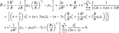 $$\begin{eqnarray}\displaystyle & & \displaystyle \ddot{R}+\frac{3}{2}\frac{{\dot{R}}^{2}}{R}-\frac{1}{\unicode[STIX]{x1D70C}R}\left[p_{b0}\left(\frac{R_{0}}{R}\right)^{3\unicode[STIX]{x1D6FE}}-p_{\infty }\right]+\frac{2\unicode[STIX]{x1D70E}}{\unicode[STIX]{x1D70C}R^{2}}+4\unicode[STIX]{x1D708}\frac{{\dot{R}}}{R^{2}}+\unicode[STIX]{x1D716}^{2}\mathop{\sum }_{n=2}^{\infty }\left\{\!\frac{1}{(2n+1)(n+1)R}\right.\nonumber\\ \displaystyle & & \displaystyle \quad \times \left.\left[\left(n+\frac{3}{2}\right){\dot{a}}_{n}^{2}+(n+3)a_{n}\ddot{a}_{n}-(n-3)\left(\frac{\ddot{R}}{R}a_{n}^{2}+\frac{1}{2}\frac{{\dot{R}}^{2}}{R^{2}}a_{n}^{2}+2\frac{{\dot{R}}}{R}a_{n}{\dot{a}}_{n}\right)\right]\!\right\}\nonumber\\ \displaystyle & & \displaystyle \quad +\,\unicode[STIX]{x1D716}^{2}\frac{1}{\unicode[STIX]{x1D70C}R^{3}}\left[p_{\infty }-p_{b0}(1-3\unicode[STIX]{x1D6FE})\left(\frac{R_{0}}{R}\right)^{3\unicode[STIX]{x1D6FE}}\right]\mathop{\sum }_{n=2}^{\infty }\frac{a_{n}^{2}}{(2n+1)}=0,\end{eqnarray}$$
and
 $$\begin{eqnarray}\displaystyle & & \displaystyle \ddot{a}_{n}+\left(\frac{3{\dot{R}}}{R}+F_{\unicode[STIX]{x1D708}}\right){\dot{a}}_{n}+(n-1)\left[(n+1)(n+2)\frac{\unicode[STIX]{x1D70E}}{\unicode[STIX]{x1D70C}R^{3}}-\frac{\ddot{R}}{R}+G_{\unicode[STIX]{x1D708}}\right]a_{n}\nonumber\\ \displaystyle & & \displaystyle \quad +\,\unicode[STIX]{x1D716}\frac{(2n+1)(n+1)}{4R}\mathop{\sum }_{i=2}^{\infty }\mathop{\sum }_{j=2}^{\infty }\left\{\frac{\ddot{R}}{R}a_{i}a_{j}G_{d_{ijn}}+\frac{{\dot{R}}^{2}}{R^{2}}a_{i}a_{j}M_{a_{nij}}\right.\nonumber\\ \displaystyle & & \displaystyle \quad +\left.\frac{{\dot{R}}}{R}a_{i}{\dot{a}}_{j}M_{b_{nij}}+a_{i}\ddot{a}_{j}M_{c_{nij}}+{\dot{a}}_{i}{\dot{a}}_{j}M_{d_{nij}}\right\}\nonumber\\ \displaystyle & & \displaystyle \quad +\,\unicode[STIX]{x1D716}\frac{(2n+1)(n+1)}{2\unicode[STIX]{x1D70C}R^{3}}\left[p_{\infty }-p_{b0}\left(\frac{R_{0}}{R}\right)^{3\unicode[STIX]{x1D6FE}}\right]\mathop{\sum }_{i=2}^{\infty }\mathop{\sum }_{j=2}^{\infty }a_{i}a_{j}I_{a_{nij}}=0,\end{eqnarray}$$
where
 $R_{0}$
is the static bubble radius,
 $\unicode[STIX]{x1D70E}$
is the surface tension,
 $\unicode[STIX]{x1D70C}$
and
 $\unicode[STIX]{x1D708}$
denotes the density and kinematic viscosity of the liquid, respectively,
 $\unicode[STIX]{x1D6FE}$
is the polytropic exponent of the gas,
 $p_{b0}$
is the equilibrium gas pressure inside the bubble defined as
 $$\begin{eqnarray}p_{b0}=p_{0}+\frac{2\unicode[STIX]{x1D70E}}{R_{0}},\end{eqnarray}$$
where
 $p_{0}$
is the static liquid pressure, and
 $p_{\infty }$
is the instantaneous liquid pressure written in the isotropic acoustic forcing assumption as
 $$\begin{eqnarray}p_{\infty }(t)=p_{0}-p_{a}\cos \unicode[STIX]{x1D714}t,\end{eqnarray}$$
where
 $p_{a}$
is the acoustic pressure amplitude and
 $\unicode[STIX]{x1D714}$
is the angular frequency. We must emphasise that viscous dissipation in the liquid has been added in a ad hoc manner in (2.2) and (2.3) by introducing the classical viscous terms to the lowest order. The viscous effects in the shape modes dynamical equation are taken into account through the well-known functions obtained in the boundary layer approximation
 $$\begin{eqnarray}\displaystyle & \displaystyle F_{\unicode[STIX]{x1D708}}=(n+2)\left[(2n+1)-2n(n+2)\frac{\unicode[STIX]{x1D6FF}}{R}\right]\frac{2\unicode[STIX]{x1D708}}{R^{2}}, & \displaystyle\end{eqnarray}$$
 $$\begin{eqnarray}\displaystyle & \displaystyle G_{\unicode[STIX]{x1D708}}=(n+2)\left[1+2n\frac{\unicode[STIX]{x1D6FF}}{R}\right]\frac{2\unicode[STIX]{x1D708}}{R^{2}}\frac{{\dot{R}}}{R}, & \displaystyle\end{eqnarray}$$
 $\unicode[STIX]{x1D6FF}=\sqrt{\unicode[STIX]{x1D708}/\unicode[STIX]{x1D714}}$
is the viscous boundary layer thickness (Brenner et al.
Reference Brenner, Lohse and Dupont1995). Note that a rigorous mathematical treatment of the liquid viscosity would lead to nonlinear viscous terms at the higher orders in (2.2) and (2.3) (Shaw Reference Shaw2009). However, as will be specified in the following, we will consider viscosity as a small perturbation so that such higher-order terms should be neglected in the further asymptotic expansion of (2.2) and (2.3) anyway. Finally, we also specify that the quantities denoted
 $I_{a}$
,
 $M_{a}$
,
 $M_{b}$
,
 $M_{c}$
,
 $M_{d}$
and
 $G_{d}$
in (2.3) involve integrals of triple products of Legendre polynomials and their derivatives. Their definitions can be found in the work of Shaw (Reference Shaw2006) and those retained in the later derivations are recalled in appendix A. These integrals can be also expressed by means of the Clebsch–Gordan coefficients (Tsamopoulos & Brown Reference Tsamopoulos and Brown1983; Doinikov Reference Doinikov2004). It is worth noting that (2.2) and (2.3) are equivalent to those derived by Doinikov (Reference Doinikov2004, equations (2.23) and (2.25)) under the assumptions of isotropic pressure forcing and negligible translational motion.
Let us now introduce new non-dimensional coordinates
 $x(t)$
and
 $s_{n}(t)$
defined as
 $$\begin{eqnarray}R(t)=R_{0}(1+x(t)),\quad a_{n}(t)=R_{0}s_{n}(t),\end{eqnarray}$$
and the new time scale
 $\unicode[STIX]{x1D70F}$
defined as
 $$\begin{eqnarray}\unicode[STIX]{x1D714}t=2\unicode[STIX]{x1D70F}.\end{eqnarray}$$
In the following, we assume that
 $x$
,
 $p_{a}$
and the squared ratio
 $(\unicode[STIX]{x1D6FF}/R_{0})^{2}$
measuring the importance of viscous damping are all small quantities of the order of
 $\unicode[STIX]{x1D716}$
. Thus performing a power series expansion of
 $x$
and neglecting terms of third and higher orders in
 $\unicode[STIX]{x1D716}$
, equations (2.2) and (2.3) become
 $$\begin{eqnarray}\displaystyle & & \displaystyle \ddot{x}+\unicode[STIX]{x1D714}_{0}^{2}x=A\cos 2\unicode[STIX]{x1D70F}+\unicode[STIX]{x1D716}(qx^{2}-{\textstyle \frac{3}{2}}{\dot{x}}^{2}-xA\cos 2\unicode[STIX]{x1D70F}-F_{\unicode[STIX]{x1D708},0}^{(0)}{\dot{x}})\nonumber\\ \displaystyle & & \displaystyle \quad +\,\unicode[STIX]{x1D716}\mathop{\sum }_{n=2}^{\infty }\frac{[(n+3)\unicode[STIX]{x1D714}_{0,n}^{2}-(n+1)\unicode[STIX]{x1D714}_{0}^{2}]s_{n}^{2}-(n+\frac{3}{2}){\dot{s}}_{n}^{2}}{(2n+1)(n+1)},\end{eqnarray}$$
and
 $$\begin{eqnarray}\displaystyle & & \displaystyle \ddot{s}_{n}+\unicode[STIX]{x1D714}_{0,n}^{2}s_{n}=\unicode[STIX]{x1D716}([(3\unicode[STIX]{x1D714}_{0,n}^{2}-(n-1)\unicode[STIX]{x1D714}_{0}^{2})x+(n-1)A\cos 2\unicode[STIX]{x1D70F}]s_{n}-3{\dot{x}}{\dot{s}}_{n}-F_{\unicode[STIX]{x1D708},0}^{(n)}{\dot{s}}_{n})\nonumber\\ \displaystyle & & \displaystyle \quad +\,\unicode[STIX]{x1D716}(2n+1)(n+1)\mathop{\sum }_{i=2}^{\infty }\mathop{\sum }_{j=2}^{\infty }\left\{\left(WI_{a_{nij}}+\unicode[STIX]{x1D714}_{0,j}^{2}\frac{M_{c_{nij}}}{4}\right)s_{i}s_{j}-\frac{M_{d_{nij}}}{4}{\dot{s}}_{i}{\dot{s}}_{j}\right\},\end{eqnarray}$$
where the dot now denotes time derivative with respect to the variable
 $\unicode[STIX]{x1D70F}$
. Several non-dimensional parameters appear in (2.9) and (2.10) which are defined as
 $$\begin{eqnarray}\displaystyle & \displaystyle A=\left(\frac{2}{\unicode[STIX]{x1D714}}\right)^{2}\frac{p_{a}}{\unicode[STIX]{x1D70C}R_{0}^{2}}, & \displaystyle\end{eqnarray}$$
 $$\begin{eqnarray}\displaystyle & \displaystyle W=\left(\frac{2}{\unicode[STIX]{x1D714}}\right)^{2}\frac{\unicode[STIX]{x1D70E}}{\unicode[STIX]{x1D70C}R_{0}^{3}}, & \displaystyle\end{eqnarray}$$
 $$\begin{eqnarray}\displaystyle & \displaystyle \unicode[STIX]{x1D714}_{0}^{2}=\left(\frac{2\unicode[STIX]{x1D6FA}_{0}}{\unicode[STIX]{x1D714}}\right)^{2}=\left(\frac{2}{\unicode[STIX]{x1D714}}\right)^{2}\frac{3\unicode[STIX]{x1D6FE}p_{b0}-2\unicode[STIX]{x1D70E}/R_{0}}{\unicode[STIX]{x1D70C}R_{0}^{2}}, & \displaystyle\end{eqnarray}$$
 $$\begin{eqnarray}\displaystyle & \displaystyle \unicode[STIX]{x1D714}_{0,n}^{2}=\left(\frac{2\unicode[STIX]{x1D6FA}_{n}}{\unicode[STIX]{x1D714}}\right)^{2}=(n-1)(n+1)(n+2)W, & \displaystyle\end{eqnarray}$$
 $$\begin{eqnarray}\displaystyle & \displaystyle q=\left(\frac{2}{\unicode[STIX]{x1D714}}\right)^{2}\frac{9\unicode[STIX]{x1D6FE}(\unicode[STIX]{x1D6FE}+1)p_{b0}/2-4\unicode[STIX]{x1D70E}/R_{0}}{\unicode[STIX]{x1D70C}R_{0}^{2}}, & \displaystyle\end{eqnarray}$$
 $$\begin{eqnarray}\displaystyle & \displaystyle F_{\unicode[STIX]{x1D708},0}^{(0)}=\left(\frac{2}{\unicode[STIX]{x1D714}}\right)\frac{4\unicode[STIX]{x1D708}}{R_{0}^{2}}=8\left(\frac{\unicode[STIX]{x1D6FF}}{R_{0}}\right)^{2}, & \displaystyle\end{eqnarray}$$
 $$\begin{eqnarray}\displaystyle & \displaystyle F_{\unicode[STIX]{x1D708},0}^{(n)}=4(n+2)\left[(2n+1)-2n(n+2)\frac{\unicode[STIX]{x1D6FF}}{R_{0}}\right]\left(\frac{\unicode[STIX]{x1D6FF}}{R_{0}}\right)^{2}. & \displaystyle\end{eqnarray}$$
 $\unicode[STIX]{x1D714}_{0}$
and the resonant frequency of the shape modes
 $\unicode[STIX]{x1D714}_{0,n}$
(Lamb Reference Lamb1932).
3 First-order solutions
We now look for solutions of (2.9) and (2.10) in the form of asymptotic expansions
 $$\begin{eqnarray}\displaystyle & \displaystyle x(\unicode[STIX]{x1D70F})=x_{0}+\unicode[STIX]{x1D716}x_{1}+\unicode[STIX]{x1D716}^{2}x_{2}+\cdots \,, & \displaystyle\end{eqnarray}$$
 $$\begin{eqnarray}\displaystyle & \displaystyle s_{n}(\unicode[STIX]{x1D70F})=s_{n,0}+\unicode[STIX]{x1D716}s_{n,1}+\unicode[STIX]{x1D716}^{2}s_{n,2}+\cdots \,. & \displaystyle\end{eqnarray}$$
Substituting (3.1) and (3.2) into (2.9) and (2.10) and equating the terms of same order in
 $\unicode[STIX]{x1D716}$
leads to the set of equations
 $$\begin{eqnarray}\displaystyle & \displaystyle \ddot{x}_{0}+\unicode[STIX]{x1D714}_{0}^{2}x_{0}=A\cos 2\unicode[STIX]{x1D70F}, & \displaystyle\end{eqnarray}$$
 $$\begin{eqnarray}\displaystyle & \displaystyle \ddot{s}_{n,0}+\unicode[STIX]{x1D714}_{0,n}^{2}s_{n,0}=0, & \displaystyle\end{eqnarray}$$
 $$\begin{eqnarray}\displaystyle \ddot{x}_{1}+\unicode[STIX]{x1D714}_{0}^{2}x_{1} & = & \displaystyle qx_{0}^{2}-{\textstyle \frac{3}{2}}{\dot{x}}_{0}^{2}-x_{0}A\cos 2\unicode[STIX]{x1D70F}-F_{\unicode[STIX]{x1D708},0}^{(0)}{\dot{x}}_{0}\nonumber\\ \displaystyle & & \displaystyle +\,\mathop{\sum }_{n=2}^{\infty }\frac{[(n+3)\unicode[STIX]{x1D714}_{0,n}^{2}-(n+1)\unicode[STIX]{x1D714}_{0}^{2}]s_{n,0}^{2}-(n+\frac{3}{2}){\dot{s}}_{n,0}^{2}}{(2n+1)(n+1)},\end{eqnarray}$$
 $$\begin{eqnarray}\displaystyle & & \displaystyle \ddot{s}_{n,1}+\unicode[STIX]{x1D714}_{0,n}^{2}s_{n,1}=[(3\unicode[STIX]{x1D714}_{0,n}^{2}-(n-1)\unicode[STIX]{x1D714}_{0}^{2})x_{0}+(n-1)A\cos 2\unicode[STIX]{x1D70F}]s_{n,0}-3{\dot{x}}_{0}{\dot{s}}_{n,0}-F_{\unicode[STIX]{x1D708},0}^{(n)}{\dot{s}}_{n,0}\nonumber\\ \displaystyle & & \displaystyle \quad +\,(2n+1)(n+1)\mathop{\sum }_{i=2}^{\infty }\mathop{\sum }_{j=2}^{\infty }\left\{\!\left(WI_{a_{nij}}+\unicode[STIX]{x1D714}_{0,j}^{2}\frac{M_{c_{nij}}}{4}\right)s_{i,0}s_{j,0}-\frac{M_{d_{nij}}}{4}{\dot{s}}_{i,0}{\dot{s}}_{j,0}\!\right\}.\end{eqnarray}$$
 $n$
close to a parametric resonance so that
 $\unicode[STIX]{x1D714}_{0,n}\simeq k$
, where
 $k$
is an integer, a suitable solution of (3.3b
) must be chosen as
 $$\begin{eqnarray}s_{n,0}=S_{n}\cos \unicode[STIX]{x1D703}_{n},\quad \text{with }\unicode[STIX]{x1D703}_{n}=k\unicode[STIX]{x1D70F}+\unicode[STIX]{x1D719}_{n}\simeq \unicode[STIX]{x1D714}_{0,n}\unicode[STIX]{x1D70F}+\unicode[STIX]{x1D719}_{n}.\end{eqnarray}$$
In the following, we limit our analysis to the first parametric resonance of the shape mode
 $n$
, thus setting
 $k=1$
. On the other hand, we consider non-resonant spherical oscillations of the bubble, sufficiently far away from the fundamental or harmonic resonances, so that
 $\unicode[STIX]{x1D714}_{0}\neq 2k$
. In the non-resonant region, the solution of (3.3a
) is written as
 $$\begin{eqnarray}x_{0}=X\cos \unicode[STIX]{x1D703}_{x},\quad \text{with }\unicode[STIX]{x1D703}_{x}=2\unicode[STIX]{x1D70F}+\unicode[STIX]{x1D719}_{x},\end{eqnarray}$$
by implicitly assuming that the steady state of the spherical oscillations is already established at the initial time. Different definitions of
 $\unicode[STIX]{x1D703}_{x}$
should be considered in the vicinity of resonances (Prosperetti Reference Prosperetti1974).
Substituting (3.5) and (3.4) into (3.3c
) and (3.3d
) produces secular terms that must be cancelled to ensure uniformly valid solutions. Depending on their respective phases
 $\unicode[STIX]{x1D703}_{i}$
and
 $\unicode[STIX]{x1D703}_{j}$
, the product of two shape modes can also produce secular terms as soon as
 $\unicode[STIX]{x1D703}_{i}-\unicode[STIX]{x1D703}_{j}\sim \unicode[STIX]{x1D703}_{n}$
or
 $\unicode[STIX]{x1D703}_{i}+\unicode[STIX]{x1D703}_{j}\sim \unicode[STIX]{x1D703}_{n}$
. Therefore, closing the formulation requires us to consider the other modes of integers
 $m\neq n$
and their respective dynamics. All these secondary modes are considered as far from their own parametric resonances, so that
 $\unicode[STIX]{x1D714}_{0,m}\neq k$
. Contrary to the parametrically forced mode
 $n$
, the modes
 $m\neq n$
are thus assumed to oscillate at the frequency of the acoustic forcing at the lowest order, and we write
 $$\begin{eqnarray}s_{m,0}=S_{m}\cos \unicode[STIX]{x1D703}_{m},\quad \text{with }\unicode[STIX]{x1D703}_{m}=2\unicode[STIX]{x1D70F}+\unicode[STIX]{x1D719}_{m}\text{ and }m\neq n.\end{eqnarray}$$
Naturally, a complete solution for a non-resonant mode
 $m$
should include a freely oscillating part, however this part would exponentially decrease due to viscous damping anyway, so (3.6) is sufficient to describe the steady state of the oscillations. The solution at first order for
 $m\neq n$
must also be solution of (3.3d
).
Following the Krylov–Bogoliubov asymptotic method (Nayfeh Reference Nayfeh2008), allowing the amplitudes
 $X$
,
 $S_{n}$
,
 $S_{m}$
and phases
 $\unicode[STIX]{x1D719}_{x}$
,
 $\unicode[STIX]{x1D719}_{n}$
,
 $\unicode[STIX]{x1D719}_{m}$
to be slowly varying functions at the time scale
 $\unicode[STIX]{x1D70F}$
and cancelling the secular terms appearing in (3.3c
) and (3.3d
) leads to the first-order differential equations
 $$\begin{eqnarray}\displaystyle & \displaystyle -4{\dot{X}}=2F_{\unicode[STIX]{x1D708},0}^{(0)}X+A\sin \unicode[STIX]{x1D719}_{x}+S_{n}^{2}\frac{\unicode[STIX]{x1D6FD}_{n}}{2}\sin (\unicode[STIX]{x1D719}_{x}-2\unicode[STIX]{x1D719}_{n}), & \displaystyle\end{eqnarray}$$
 $$\begin{eqnarray}\displaystyle & \displaystyle -4X\dot{\unicode[STIX]{x1D719}}_{x}=(4-\unicode[STIX]{x1D714}_{0}^{2})X+A\cos \unicode[STIX]{x1D719}_{x}+S_{n}^{2}\frac{\unicode[STIX]{x1D6FD}_{n}}{2}\cos (\unicode[STIX]{x1D719}_{x}-2\unicode[STIX]{x1D719}_{n}), & \displaystyle\end{eqnarray}$$
 $$\begin{eqnarray}\displaystyle -2{\dot{S}}_{n} & = & \displaystyle F_{\unicode[STIX]{x1D708},0}^{(n)}S_{n}+\frac{S_{n}}{2}\left(\unicode[STIX]{x1D6FE}_{n}X\sin (2\unicode[STIX]{x1D719}_{n}-\unicode[STIX]{x1D719}_{x})+(n-1)A\sin 2\unicode[STIX]{x1D719}_{n}\right.\nonumber\\ \displaystyle & & \displaystyle +\left.\mathop{\sum }_{m\neq n}W_{nm}S_{m}\sin (2\unicode[STIX]{x1D719}_{n}-\unicode[STIX]{x1D719}_{m})\right),\end{eqnarray}$$
 $$\begin{eqnarray}\displaystyle -2S_{n}\dot{\unicode[STIX]{x1D719}}_{n} & = & \displaystyle (1-\unicode[STIX]{x1D714}_{0,n}^{2})S_{n}+\frac{S_{n}}{2}\left(\unicode[STIX]{x1D6FE}_{n}X\cos (2\unicode[STIX]{x1D719}_{n}-\unicode[STIX]{x1D719}_{x})+(n-1)A\cos 2\unicode[STIX]{x1D719}_{n}\right.\nonumber\\ \displaystyle & & \displaystyle +\left.\mathop{\sum }_{m\neq n}W_{nm}S_{m}\cos (2\unicode[STIX]{x1D719}_{n}-\unicode[STIX]{x1D719}_{m})\right),\end{eqnarray}$$
 $$\begin{eqnarray}\displaystyle & \displaystyle -4{\dot{S}}_{m}=2F_{\unicode[STIX]{x1D708},0}^{(m)}S_{m}+O_{mn}\frac{S_{n}^{2}}{2}\sin (\unicode[STIX]{x1D719}_{m}-2\unicode[STIX]{x1D719}_{n}), & \displaystyle\end{eqnarray}$$
 $$\begin{eqnarray}\displaystyle & \displaystyle -4S_{m}\dot{\unicode[STIX]{x1D719}}_{m}=(4-\unicode[STIX]{x1D714}_{0,m}^{2})S_{m}+O_{mn}\frac{S_{n}^{2}}{2}\cos (\unicode[STIX]{x1D719}_{m}-2\unicode[STIX]{x1D719}_{n}), & \displaystyle\end{eqnarray}$$
 $\unicode[STIX]{x1D6FD}_{n}$
,
 $\unicode[STIX]{x1D6FE}_{n}$
,
 $W_{nm}$
and
 $O_{mn}$
are summarised in appendix A. The solutions of (3.3c
) and (3.3d
) free of secular terms are then given by
 $$\begin{eqnarray}\displaystyle x_{1} & = & \displaystyle \frac{X}{\unicode[STIX]{x1D714}_{0}^{2}}\left(\left[\frac{q}{2}-3\right]X-\frac{A}{2}\cos \unicode[STIX]{x1D719}_{x}\right)\nonumber\\ \displaystyle & & \displaystyle +\,\frac{X}{\unicode[STIX]{x1D714}_{0}^{2}-16}\left(\left[\frac{q}{2}+3\right]X\cos (4\unicode[STIX]{x1D70F}+2\unicode[STIX]{x1D719}_{x})-\frac{A}{2}\cos (4\unicode[STIX]{x1D70F}+\unicode[STIX]{x1D719}_{x})\right)\nonumber\\ \displaystyle & & \displaystyle +\,\unicode[STIX]{x1D714}_{0}^{-2}\unicode[STIX]{x1D6FC}_{n}\frac{S_{n}^{2}}{2}+\mathop{\sum }_{m\neq n}^{\infty }\frac{S_{m}^{2}}{2}(\unicode[STIX]{x1D714}_{0}^{-2}\unicode[STIX]{x1D6FC}_{m}+(\unicode[STIX]{x1D714}_{0}^{2}-16)^{-1}\unicode[STIX]{x1D6FD}_{m}\cos (4\unicode[STIX]{x1D70F}+2\unicode[STIX]{x1D719}_{m})),\end{eqnarray}$$
 $$\begin{eqnarray}\displaystyle s_{n,1} & = & \displaystyle \frac{S_{n}}{2(\unicode[STIX]{x1D714}_{0,n}^{2}-9)}(\unicode[STIX]{x1D6FF}_{n}X\cos (3\unicode[STIX]{x1D70F}+\unicode[STIX]{x1D719}_{n}+\unicode[STIX]{x1D719}_{x})+(n-1)A\cos (3\unicode[STIX]{x1D70F}+\unicode[STIX]{x1D719}_{n}))\nonumber\\ \displaystyle & & \displaystyle +\,\frac{(2n+1)(n+1)}{8}\left\{S_{n}^{2}\left[\frac{J_{a_{nnn}}-M_{d_{nnn}}}{\unicode[STIX]{x1D714}_{0,n}^{2}}+\frac{J_{a_{nnn}}+M_{d_{nnn}}}{\unicode[STIX]{x1D714}_{0,n}^{2}-4}\cos (2\unicode[STIX]{x1D70F}+2\unicode[STIX]{x1D719}_{n})\right]\right.\nonumber\\ \displaystyle & & \displaystyle +\,\mathop{\sum }_{i\neq n}\mathop{\sum }_{j\neq n}S_{i}S_{j}\left[\frac{J_{a_{nij}}-4M_{d_{nij}}}{\unicode[STIX]{x1D714}_{0,n}^{2}}\cos (\unicode[STIX]{x1D719}_{i}-\unicode[STIX]{x1D719}_{j})+\frac{J_{a_{nij}}+4M_{d_{nij}}}{\unicode[STIX]{x1D714}_{0,n}^{2}-16}\cos (4\unicode[STIX]{x1D70F}+\unicode[STIX]{x1D719}_{i}+\unicode[STIX]{x1D719}_{j})\right]\nonumber\\ \displaystyle & & \displaystyle +\left.\mathop{\sum }_{i\neq n}S_{i}S_{n}\frac{J_{a_{nin}}+J_{a_{nni}}+2(M_{d_{nin}}+M_{d_{nni}})}{\unicode[STIX]{x1D714}_{0,n}^{2}-9}\cos (3\unicode[STIX]{x1D70F}+\unicode[STIX]{x1D719}_{i}+\unicode[STIX]{x1D719}_{n})\right\},\end{eqnarray}$$
 $$\begin{eqnarray}\displaystyle s_{m,1} & = & \displaystyle \frac{S_{m}}{2\unicode[STIX]{x1D714}_{0,m}^{2}}(\unicode[STIX]{x1D6FE}_{m}X\cos (\unicode[STIX]{x1D719}_{m}-\unicode[STIX]{x1D719}_{x})+(m-1)A\cos \unicode[STIX]{x1D719}_{m})\nonumber\\ \displaystyle & & \displaystyle +\,\frac{S_{m}}{2(\unicode[STIX]{x1D714}_{0,m}^{2}-16)}(\unicode[STIX]{x1D6FF}_{m}X\cos (4\unicode[STIX]{x1D70F}+\unicode[STIX]{x1D719}_{m}+\unicode[STIX]{x1D719}_{x})+(m-1)A\cos (4\unicode[STIX]{x1D70F}+\unicode[STIX]{x1D719}_{m}))\nonumber\\ \displaystyle & & \displaystyle +\,\frac{(2m+1)(m+1)}{8}\left\{S_{n}^{2}(J_{a_{mnn}}-M_{d_{mnn}})\unicode[STIX]{x1D714}_{0,m}^{-2}\right.\nonumber\\ \displaystyle & & \displaystyle +\,\mathop{\sum }_{i\neq n}\mathop{\sum }_{j\neq n}S_{i}S_{j}\left[\frac{J_{a_{mij}}-4M_{d_{mij}}}{\unicode[STIX]{x1D714}_{0,m}^{2}}\cos (\unicode[STIX]{x1D719}_{i}-\unicode[STIX]{x1D719}_{j})+\frac{J_{a_{mij}}+4M_{d_{mij}}}{\unicode[STIX]{x1D714}_{0,m}^{2}-16}\cos (4\unicode[STIX]{x1D70F}+\unicode[STIX]{x1D719}_{i}+\unicode[STIX]{x1D719}_{j})\right]\nonumber\\ \displaystyle & & \displaystyle +\,\mathop{\sum }_{i\neq n}S_{i}S_{n}\frac{J_{a_{min}}+J_{a_{mni}}-2(M_{d_{min}}+M_{d_{mni}})}{\unicode[STIX]{x1D714}_{0,m}^{2}-1}\cos (\unicode[STIX]{x1D70F}+\unicode[STIX]{x1D719}_{i}-\unicode[STIX]{x1D719}_{n})\nonumber\\ \displaystyle & & \displaystyle +\left.\mathop{\sum }_{i\neq n}S_{i}S_{n}\frac{J_{a_{min}}+J_{a_{mni}}+2(M_{d_{min}}+M_{d_{mni}})}{\unicode[STIX]{x1D714}_{0,m}^{2}-9}\cos (3\unicode[STIX]{x1D70F}+\unicode[STIX]{x1D719}_{i}+\unicode[STIX]{x1D719}_{n})\right\},\end{eqnarray}$$
where the coefficients
 $\unicode[STIX]{x1D6FC}_{n}$
,
 $\unicode[STIX]{x1D6FF}_{n}$
and
 $J_{a_{nij}}$
are also summarised in appendix A.
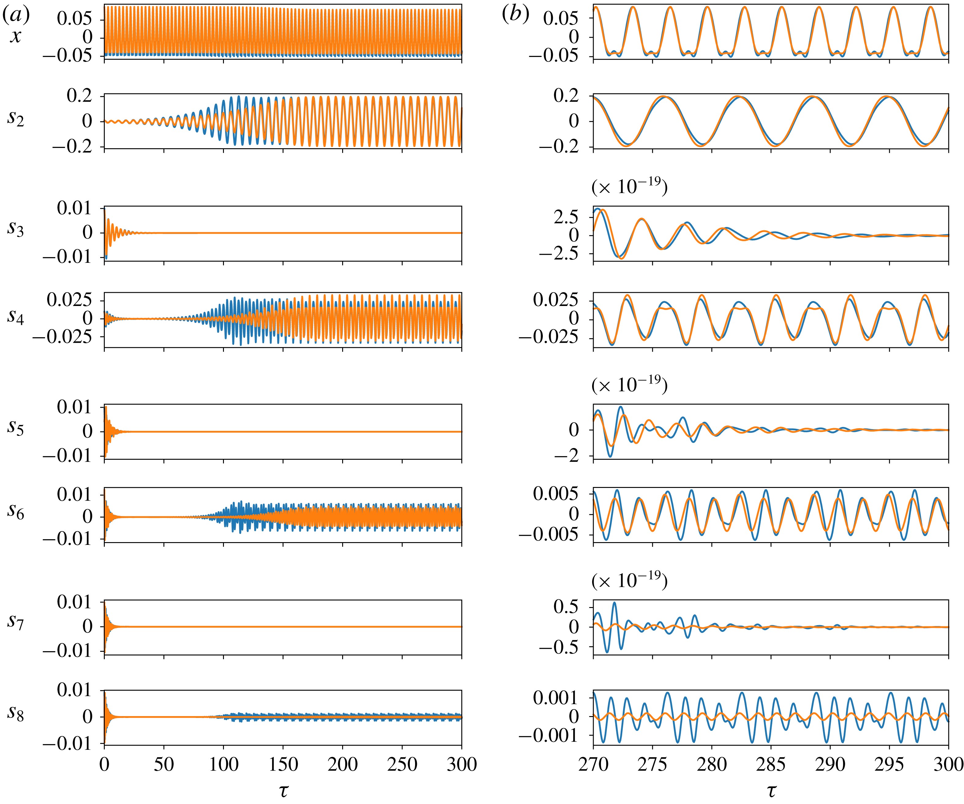
Oscillations of the spherical mode and the seven first shape modes for a bubble of radius
 $R_{0}=44.8~\unicode[STIX]{x03BC}\text{m}$
driven above the first parametric resonance of the
 $n=2$
mode (
 $\unicode[STIX]{x1D714}/(2\unicode[STIX]{x03C0})=31.25~\text{kHz}$
,
 $P_{a}=22.25~\text{kPa}$
,
 $\unicode[STIX]{x1D714}_{0,2}\sim 1$
, corresponding to the point
 $\triangledown$
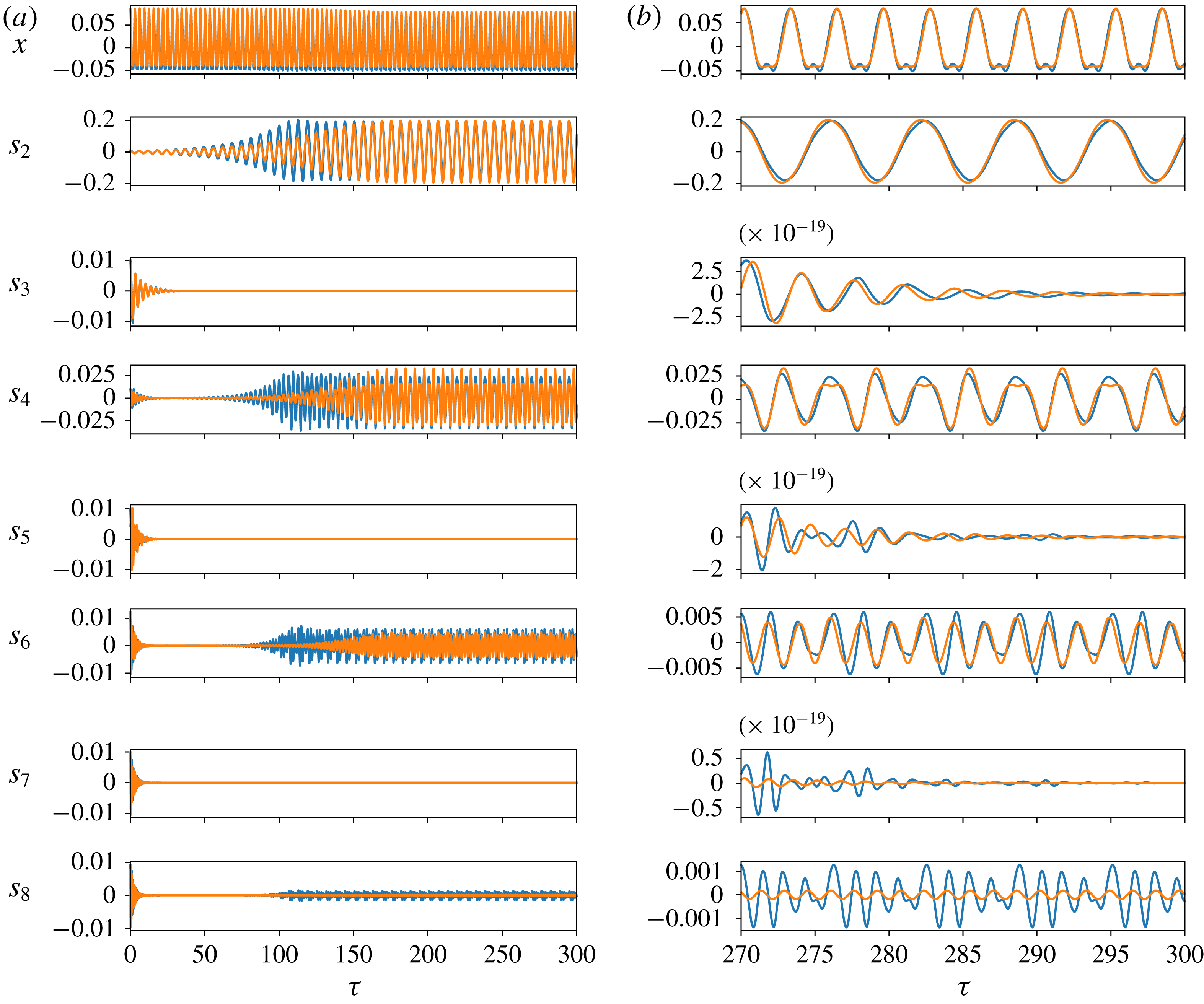
in figure 5). Numerical simulations (blue curves) are compared with first-order approximate solutions (orange curves). (a) Presents the results over long times, from transient oscillations to the establishment of the steady-state regime. (b) Focuses on few acoustic periods during the steady state.
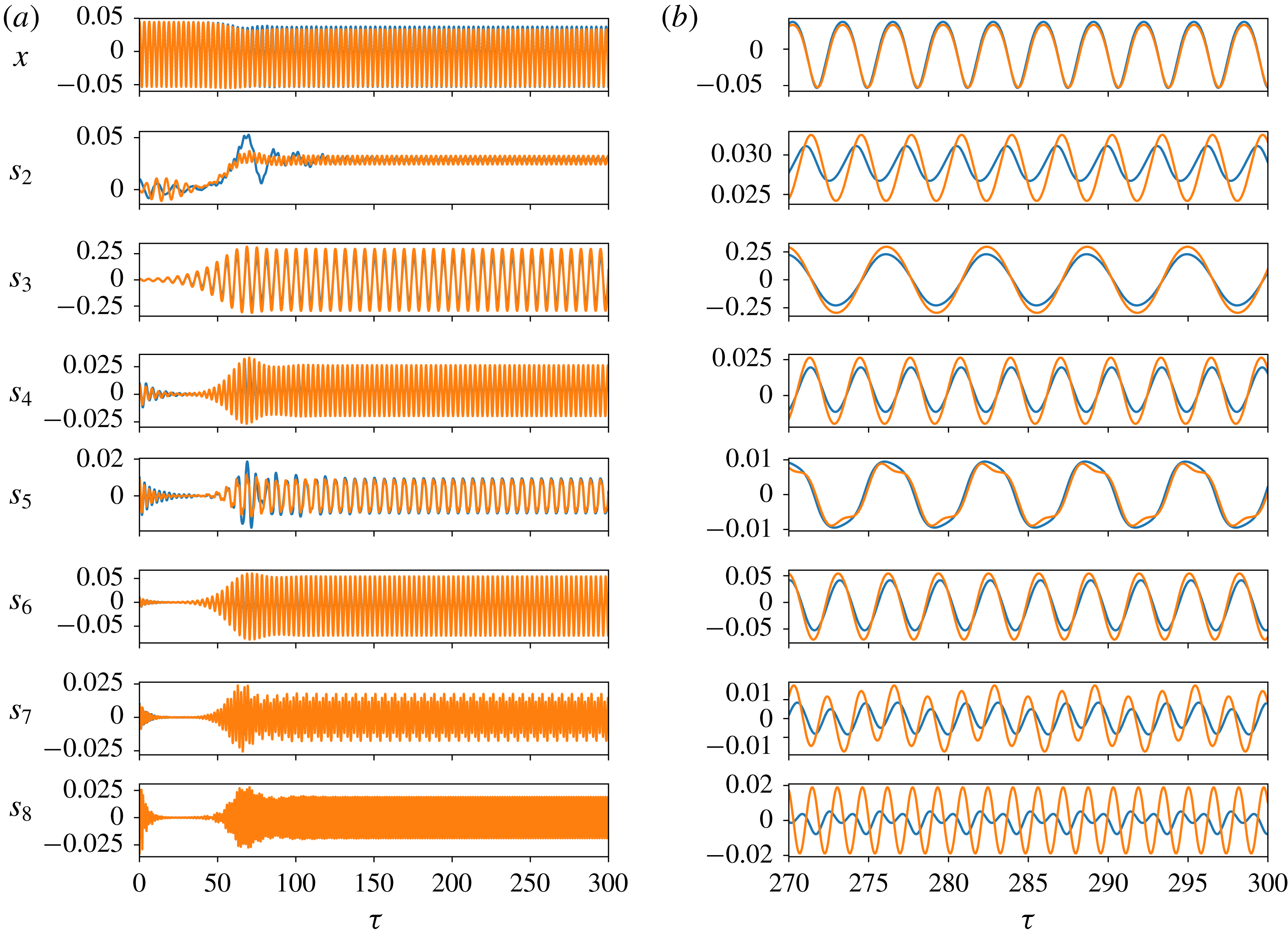
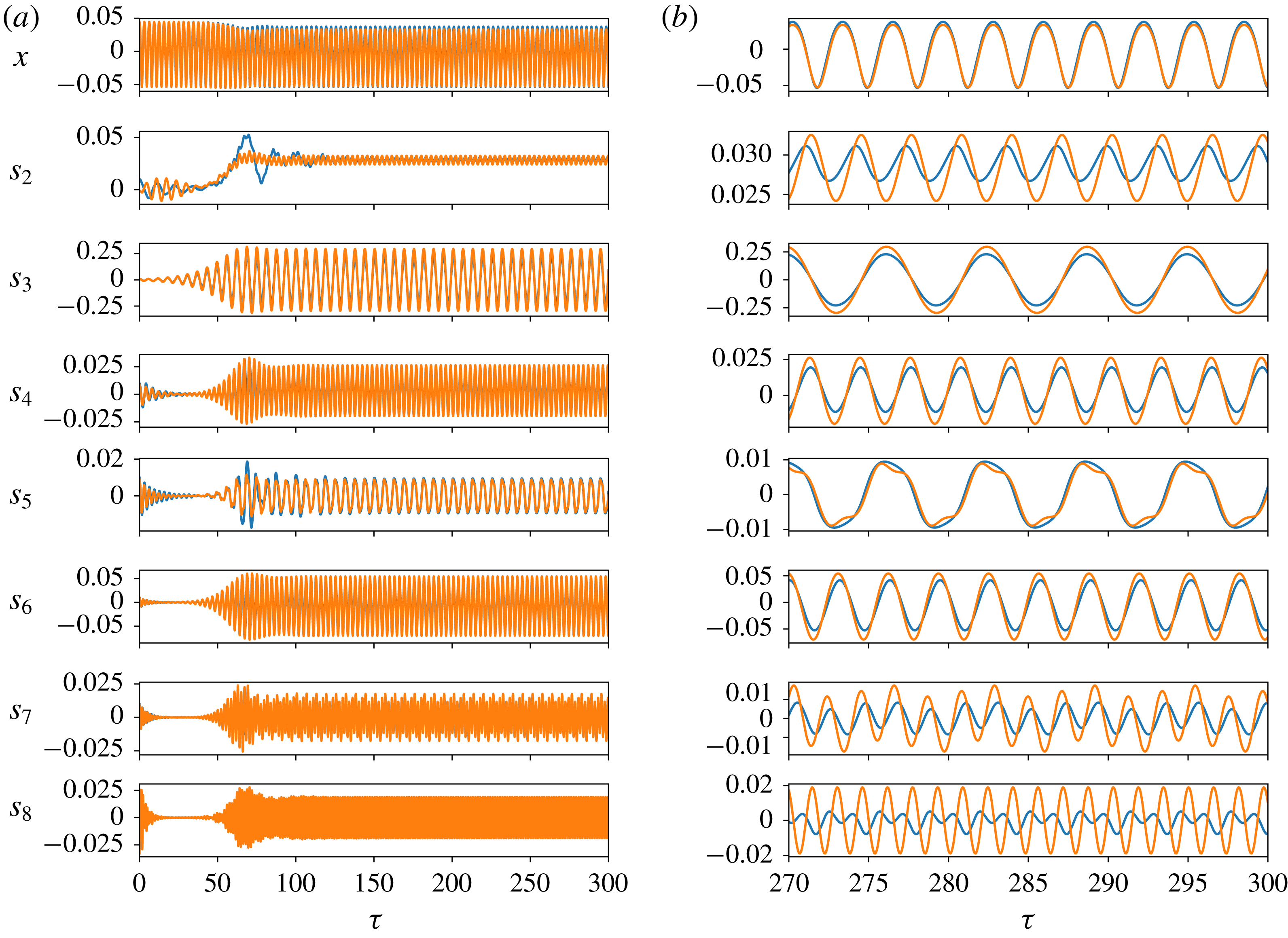
Same as figure 1, for a bubble of radius
 $R_{0}=66.9~\unicode[STIX]{x03BC}\text{m}$
driven above the first parametric resonance of the
 $n=3$
mode (
 $\unicode[STIX]{x1D714}/(2\unicode[STIX]{x03C0})=31.25~\text{kHz}$
,
 $P_{a}=12.69~\text{kPa}$
,
 $\unicode[STIX]{x1D714}_{0,3}\sim 1$
, corresponding to the point ▫ in figure 6).
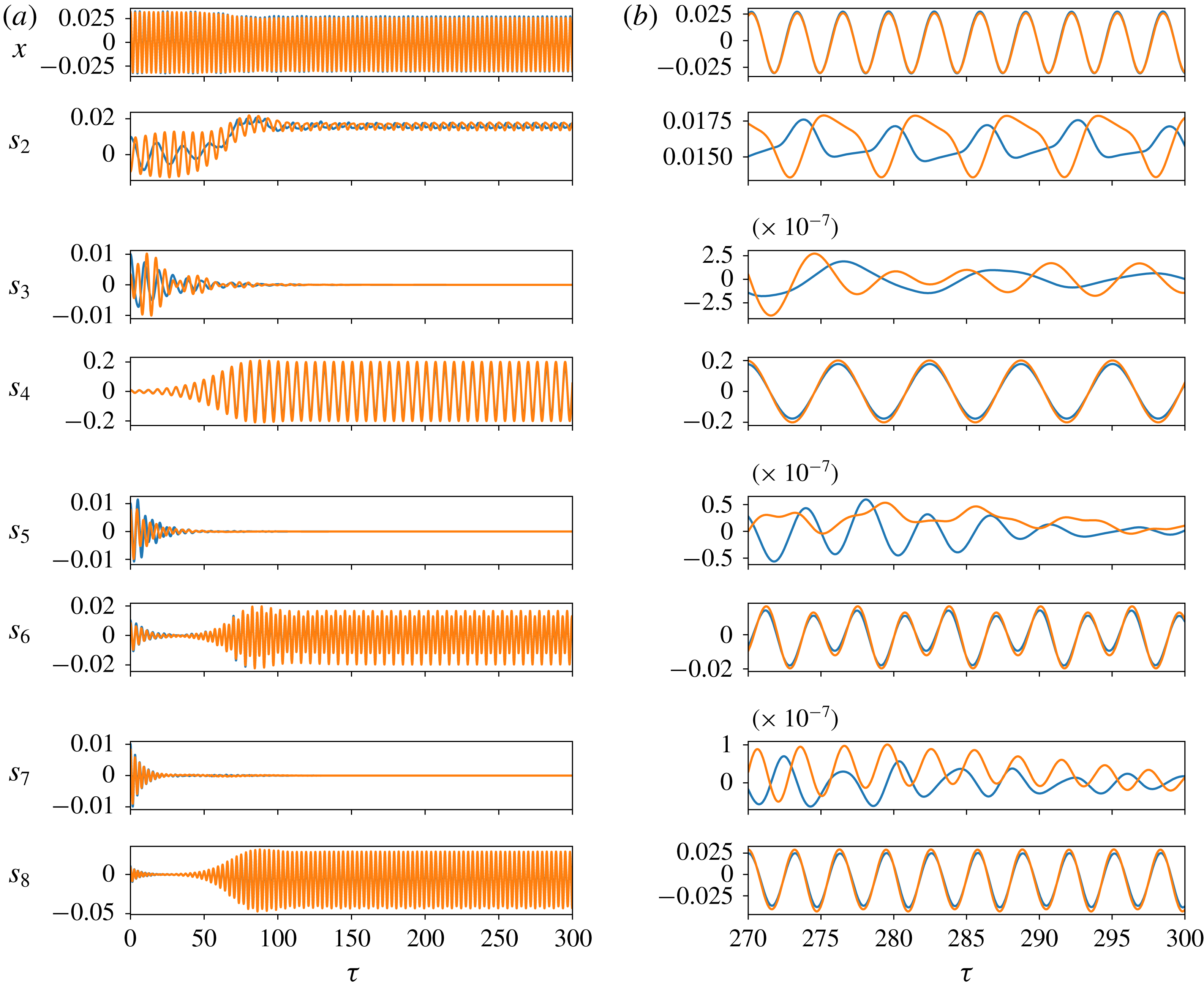
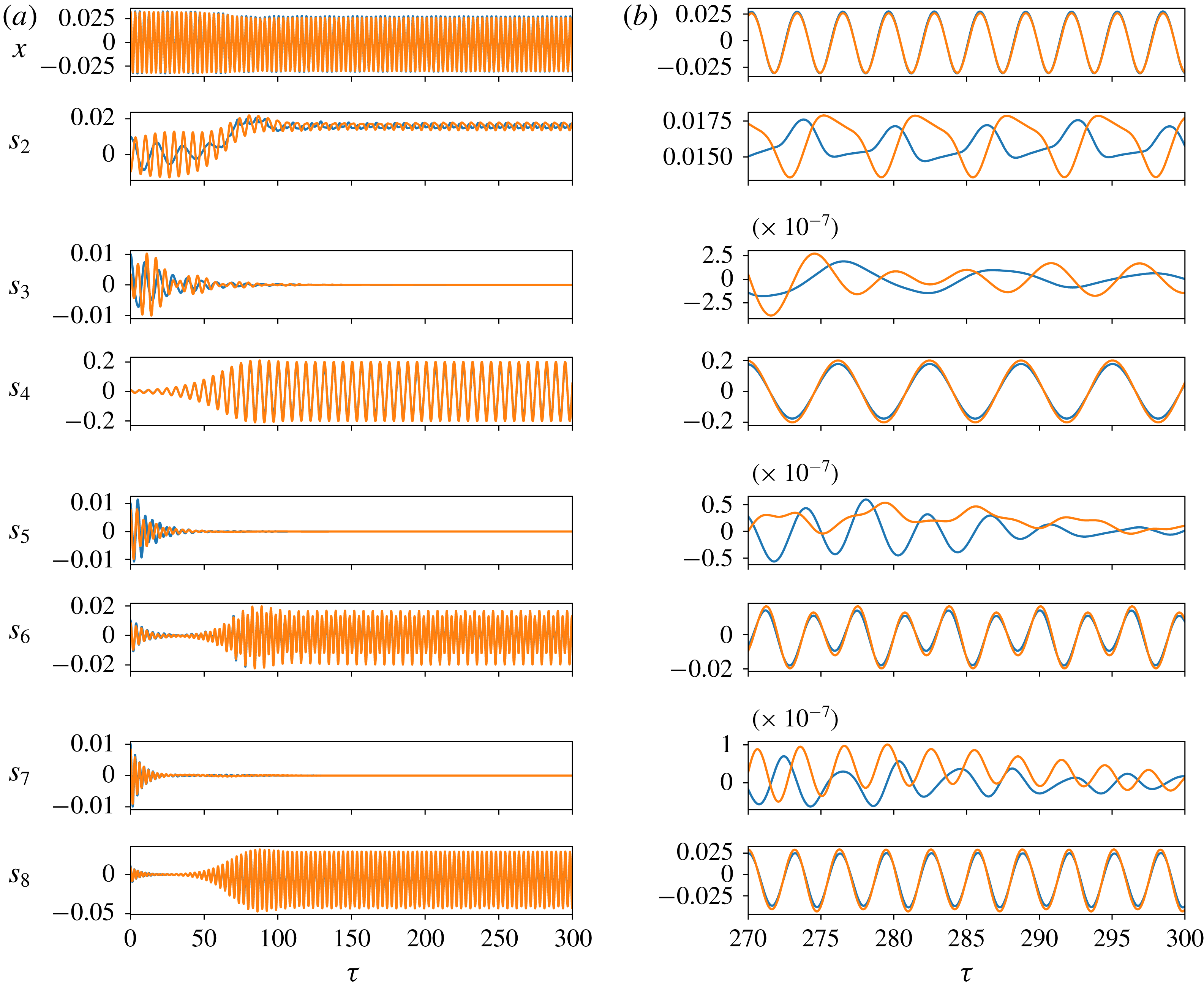
Same as figure 1, for a bubble of radius
 $R_{0}=90.72~\unicode[STIX]{x03BC}\text{m}$
driven above the first parametric resonance of the
 $n=4$
mode (
 $\unicode[STIX]{x1D714}/(2\unicode[STIX]{x03C0})=31.25~\text{kHz}$
,
 $P_{a}=3.62~\text{kPa}$
,
 $\unicode[STIX]{x1D714}_{0,4}\sim 0.95$
, corresponding to the point ▿ in figure 7).
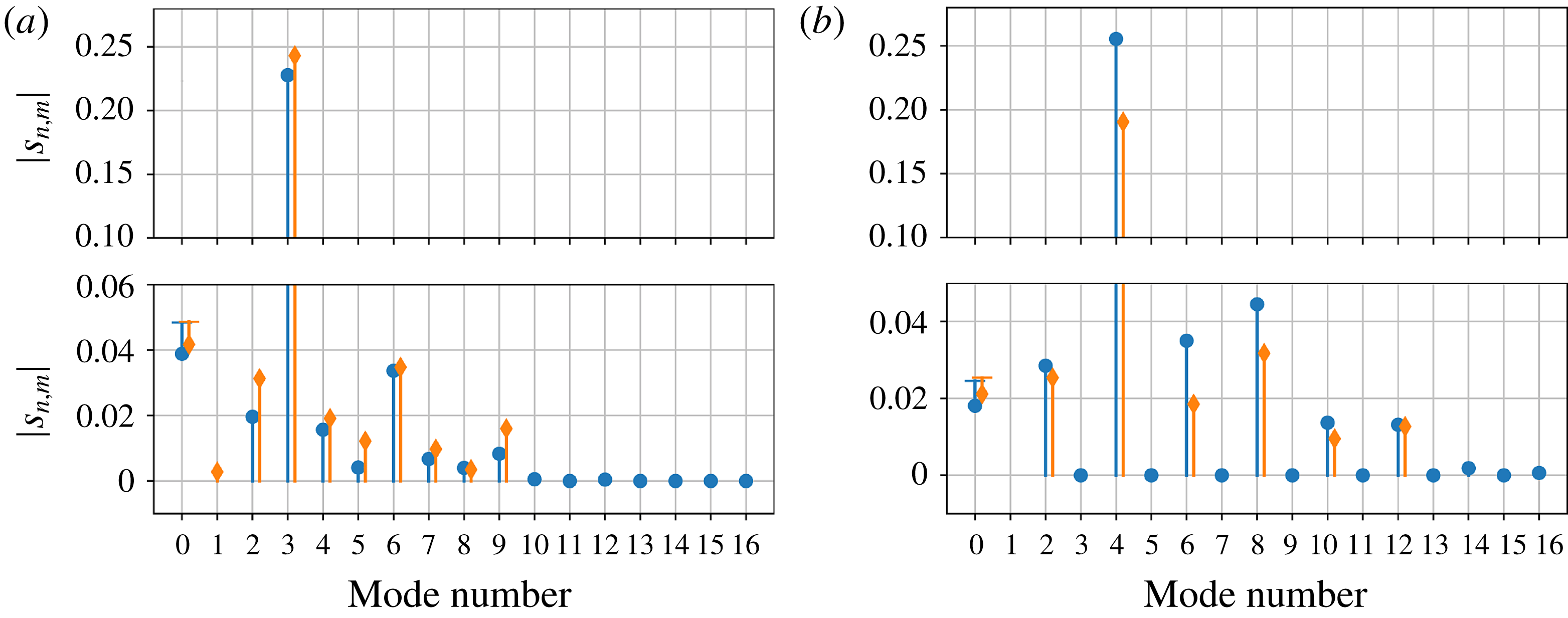
Modal amplitudes including the spherical (
 $0$
) and translational (
 $1$
) vibrational modes, for two bubbles driven at
 $\unicode[STIX]{x1D714}/(2\unicode[STIX]{x03C0})=10~\text{kHz}$
. (a)
 $R_{0}=144~\unicode[STIX]{x03BC}\text{m}$
,
 $P_{a}=13~\text{kPa}$
,
 $\unicode[STIX]{x1D714}_{0,3}\sim 0.99$
. (b)
 $R_{0}=189~\unicode[STIX]{x03BC}\text{m}$
,
 $P_{a}=8~\text{kPa}$
,
 $\unicode[STIX]{x1D714}_{0,4}\sim 0.99$
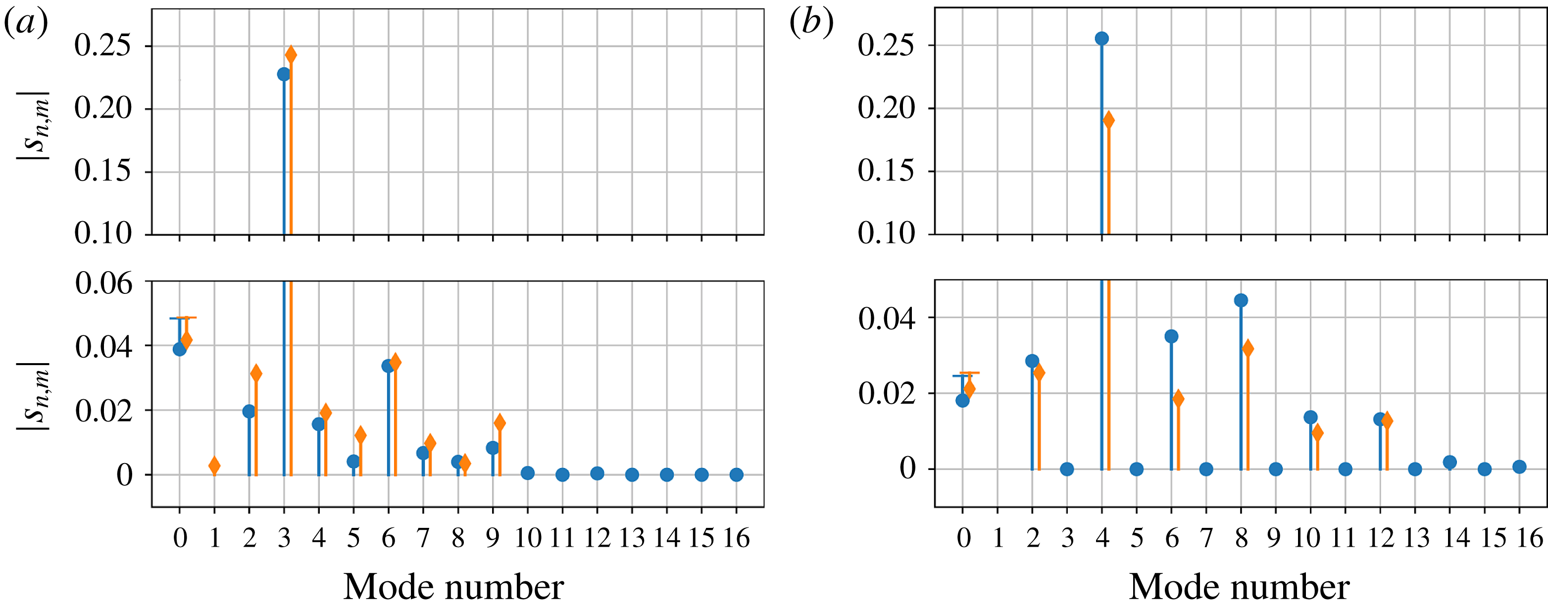
. Circles (○) correspond to results from the Krylov–Bogoliubov perturbation method, while diamonds (♢) correspond to amplitudes in steady state obtained from the numerical simulations presented in the paper of Shaw (Reference Shaw2017). For the spherical mode, we represent the difference between the amplitude before (
 $-$
) and after (symbol) the establishment of the surface oscillations. Sustaining shape oscillations generally goes with a decreasing of the amplitude of the spherical oscillations.
The approximate solutions (3.5)–(3.6) and (3.8)–(3.10) are compared to the direct numerical integration of (2.2) and (2.3) in figures 1–3, for the parametric excitation of the first three shape modes
 $n=2$
,
 $n=3$
and
 $n=4$
, respectively. We consider air bubbles of typical radii around
 $R_{0}\simeq 50{-}90~\unicode[STIX]{x03BC}\text{m}$
in water, driven by an external forcing at frequency
 $\unicode[STIX]{x1D714}/(2\unicode[STIX]{x03C0})=31.25~\text{kHz}$
, following experimental conditions available in the literature (Guédra et al.
Reference Guédra, Cleve, Mauger, Blanc-Benon and Inserra2017). Eight modes are retained in the computation. The initial conditions for all shape modes are set to
 $s_{n}(0)=s_{m}(0)=10^{-2}$
and
 ${\dot{s}}_{n}(0)={\dot{s}}_{m}(0)=0$
, while the steady state of the spherical oscillations is already established at initial time as mentioned previously (a simulation of the Rayleigh–Plesset equation has been run prior to the calculation to set the initial conditions for
 $x$
and
 ${\dot{x}}$
). The simulations are then performed over 100 periods, corresponding to a total time of 3.2 ms.
Looking at the general dynamics shown in figures 1–3 first indicates that the equations obtained from the perturbation method reproduce the characteristic exponential growth of the instability and capture the nonlinear saturation of the shape modes. Finally, the steady-state regime with finite-amplitude oscillations is recovered. The unstable shape mode close to its first parametric resonance naturally oscillates mainly at half the driving frequency (
 $\unicode[STIX]{x1D714}_{0,n}\simeq 1$
). The approximate solutions, through the differential set of equations (3.7a–f
), also capture the exponential decay of damped non-resonant shape modes (being roughly of the type
 $S_{m}\propto \exp [-F_{\unicode[STIX]{x1D708},0}^{(m)}\unicode[STIX]{x1D70F}/2]$
) as well as the possible excitation of some particular shape modes coming from nonlinear coupling. The presence or absence of shape modes is ruled by the values of
 $W_{mn}$
and
 $O_{nm}$
involved in (3.7a–f
), which can be zero for particular
 $(n,m)$
combinations. Comparing figures 1 to 3 notably illustrates that parametrically forced even modes are only able to excite other even modes (at least at this order of approximation), while odd modes can excite both even and odd modes (Shaw Reference Shaw2006). These results also highlight the important drift effect observed for the
 $s_{2}$
shape mode in figures 2 and 3 coming from the non-oscillating terms in (3.10). This effect is a typical signature of nonlinear mode coupling and has already been observed both experimentally by Guédra et al. (Reference Guédra, Inserra, Mauger and Gilles2016b
) and numerically by Shaw (Reference Shaw2017).
In figure 4, the approximate solutions are compared to a more complete theory derived by Shaw (Reference Shaw2017) including translational motion and liquid compressibility up to third order. The calculations are made for a driving frequency
 $\unicode[STIX]{x1D714}/(2\unicode[STIX]{x03C0})=10~\text{kHz}$
, in the vicinity of the first parametric resonance of the shape modes
 $n=3$
(i) and
 $n=4$
(ii), referring to the figures 5–6 and 9–10 presented in the paper of Shaw (Reference Shaw2017). The steady-state amplitudes are given as a function of the mode number, up to 16 modes retained for computation. Even with several assumptions made in the perturbation analysis, the general trend is satisfactory. Moreover, these results highlight the decreasing amplitude of the spherical solution (mode
 $0$
) due to the triggering of non-spherical oscillations. This specific influence of shape modes on the spherical one will be further commented on in the next section.
Finally, we must also pay attention to the boundary layer approximation used to introduce viscous dissipation in the present model. This assumption should be used with caution as it discards the continuous diffusion of vorticity by viscosity (Prosperetti Reference Prosperetti1977) which leads to increasing the boundary layer on long times. The importance of vorticity effects can be inferred from the estimate of the characteristic time
 $R_{0}^{2}/\unicode[STIX]{x1D708}$
representative of viscous diffusion. This time ranges from 2.5 to 8 ms for the micrometre-sized bubbles considered in our simulations, which is comparable to the total computation time and cannot be strictly considered as much larger than the time required for the growth and saturation of the surface oscillations. Moreover an estimate of the Reynolds number from the calculation of the characteristic capillary time leads to values as low as
 $Re\simeq 85$
, which indicates that viscous effects are probably underestimated by the boundary layer approximation. For the bubbles considered in the simulations, it can in fact be expected that stronger viscous damping can participate in the saturation of the shape oscillations to a similar extent as nonlinear mode coupling. Thus a quantitative comparison with experimental data would certainly require a more rigorous mathematical treatment of the viscous terms, notably accounting for the growth of the viscous layer convected by vorticity as considered in the works of Lundgren & Mansour (Reference Lundgren and Mansour1988).
4 Steady-state solutions
In the previous section, the temporal dynamics obtained from numerical integration revealed that nonlinear mode coupling is responsible for a saturation of the instability leading to stable non-spherical oscillations. In order to obtain the corresponding steady-state solutions, the set of differential equations (3.7a–f
) is first put in a more convenient complex form by introducing the complex variables
 $\bar{X}=X\text{e}^{\text{i}\unicode[STIX]{x1D719}_{x}}$
,
 $\bar{S_{n}}=S_{n}\text{e}^{\text{i}\unicode[STIX]{x1D719}_{n}}$
and
 $\bar{S_{m}}=S_{m}\text{e}^{\text{i}\unicode[STIX]{x1D719}_{m}}$
to obtain
 $$\begin{eqnarray}\displaystyle & \displaystyle 4\text{i}\dot{\bar{X}}=\bar{\unicode[STIX]{x1D6E5}}_{0}\bar{X}+A+\frac{\unicode[STIX]{x1D6FD}_{n}}{2}\bar{S}_{n}^{2}, & \displaystyle\end{eqnarray}$$
 $$\begin{eqnarray}\displaystyle & \displaystyle 2\text{i}\dot{\bar{S}}_{n}=\bar{\unicode[STIX]{x1D6E5}}_{n}\bar{S}_{n}+\left(\unicode[STIX]{x1D6FE}_{n}\bar{X}+(n-1)A+\mathop{\sum }_{m\neq n}W_{nm}\bar{S}_{m}\right)\frac{{\bar{S}_{n}}^{\ast }}{2}, & \displaystyle\end{eqnarray}$$
 $$\begin{eqnarray}\displaystyle & \displaystyle 4\text{i}\dot{\bar{S}}_{m}=\bar{\unicode[STIX]{x1D6E5}}_{m}\bar{S}_{m}+O_{mn}\frac{\bar{S}_{n}^{2}}{2}, & \displaystyle\end{eqnarray}$$
 $\ast$
denotes the conjugate, and the complex quantities
 $\bar{\unicode[STIX]{x1D6E5}}$
are defined by
 $$\begin{eqnarray}\displaystyle & \displaystyle \bar{\unicode[STIX]{x1D6E5}}_{0}=(4-\unicode[STIX]{x1D714}_{0}^{2})-2\text{i}F_{\unicode[STIX]{x1D708},0}^{(0)}, & \displaystyle\end{eqnarray}$$
 $$\begin{eqnarray}\displaystyle & \displaystyle \bar{\unicode[STIX]{x1D6E5}}_{n}=(1-\unicode[STIX]{x1D714}_{0,n}^{2})-\text{i}F_{\unicode[STIX]{x1D708},0}^{(n)}, & \displaystyle\end{eqnarray}$$
 $$\begin{eqnarray}\displaystyle & \displaystyle \bar{\unicode[STIX]{x1D6E5}}_{m}=(4-\unicode[STIX]{x1D714}_{0,m}^{2})-2\text{i}F_{\unicode[STIX]{x1D708},0}^{(m)}. & \displaystyle\end{eqnarray}$$
In the steady-state regime, cancelling the first temporal derivatives in (4.1a ) and (4.1c ) directly provides the complex amplitudes of the spherical and secondary shape modes
 $$\begin{eqnarray}\displaystyle & \displaystyle \bar{X}=-\bar{\unicode[STIX]{x1D6E5}}_{0}^{-1}\left(A+\frac{\unicode[STIX]{x1D6FD}_{n}}{2}\bar{S}_{n}^{2}\right), & \displaystyle\end{eqnarray}$$
 $$\begin{eqnarray}\displaystyle & \displaystyle \bar{S}_{m}=-\bar{\unicode[STIX]{x1D6E5}}_{m}^{-1}O_{mn}\frac{\bar{S}_{n}^{2}}{2}. & \displaystyle\end{eqnarray}$$
Then substituting (4.5) and (4.6) into (4.1b ) leads to the equation
 $$\begin{eqnarray}\left(2\bar{\unicode[STIX]{x1D6E5}}_{n}-\frac{S_{n}^{2}}{2}\left(\frac{\unicode[STIX]{x1D6FE}_{n}\unicode[STIX]{x1D6FD}_{n}}{\bar{\unicode[STIX]{x1D6E5}}_{0}}+\mathop{\sum }_{m\neq n}\frac{W_{nm}O_{mn}}{\bar{\unicode[STIX]{x1D6E5}}_{m}}\right)\right)\bar{S}_{n}=-\!\left((n-1)-\frac{\unicode[STIX]{x1D6FE}_{n}}{\bar{\unicode[STIX]{x1D6E5}}_{0}}\right)A{\bar{S}_{n}}^{\ast },\end{eqnarray}$$
which has the trivial solution
 $S_{n}=0$
(with undetermined phase
 $\unicode[STIX]{x1D719}_{n}$
), and solutions ruled by
 $$\begin{eqnarray}\displaystyle & \displaystyle \left|\bar{h}_{1}-\frac{S_{n}^{2}}{2}\bar{h}_{2}\right|=|\bar{h}_{3}|A, & \displaystyle\end{eqnarray}$$
 $$\begin{eqnarray}\displaystyle & \displaystyle \text{e}^{2\text{i}\unicode[STIX]{x1D719}_{n}}=-\frac{\bar{h}_{3}A}{\displaystyle \bar{h}_{1}-\frac{S_{n}^{2}}{2}\bar{h}_{2}}, & \displaystyle\end{eqnarray}$$
where we have introduced the complex quantities
 $$\begin{eqnarray}\displaystyle & \displaystyle \bar{h}_{1}=2\bar{\unicode[STIX]{x1D6E5}}_{n}, & \displaystyle\end{eqnarray}$$
 $$\begin{eqnarray}\displaystyle & \displaystyle \bar{h}_{2}=\bar{\unicode[STIX]{x1D6E5}}_{0}^{-1}\unicode[STIX]{x1D6FE}_{n}\unicode[STIX]{x1D6FD}_{n}+\mathop{\sum }_{m\neq n}\bar{\unicode[STIX]{x1D6E5}}_{m}^{-1}W_{nm}O_{mn}, & \displaystyle\end{eqnarray}$$
 $$\begin{eqnarray}\displaystyle & \displaystyle \bar{h}_{3}=(n-1)-\bar{\unicode[STIX]{x1D6E5}}_{0}^{-1}\unicode[STIX]{x1D6FE}_{n}, & \displaystyle\end{eqnarray}$$
for the conciseness of the derivations.
Driving amplitude as a function of the frequency
 $\unicode[STIX]{x1D714}_{0,n}$
, for
 $n=2$
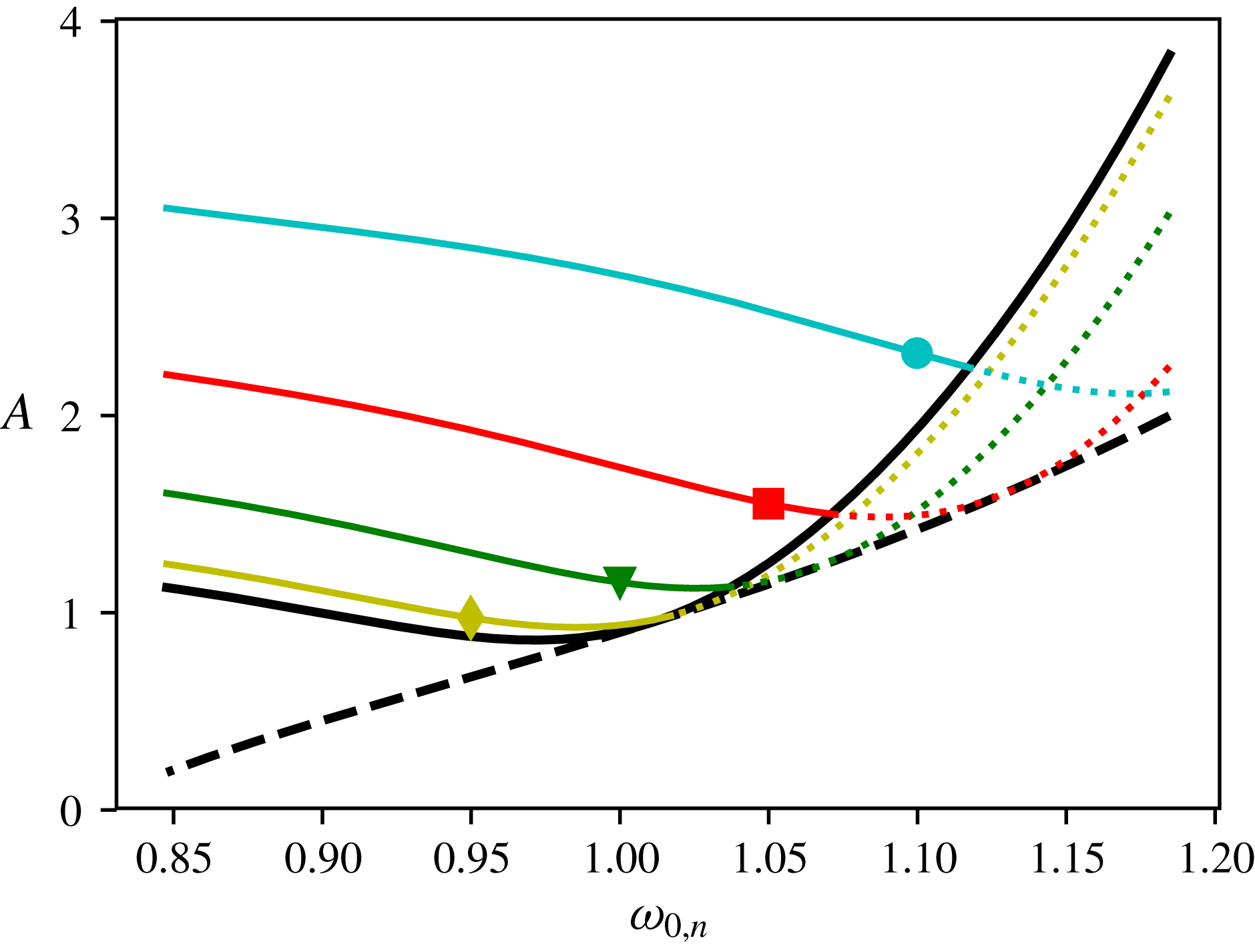
. The absolute stability threshold computed from (4.13) is given by the thick curve. The conditional stability threshold computed from (4.17) is given by the dashed curve. The other curves are isolines corresponding to fixed values of
 $S_{n}$
in steady state:
 $S_{n}=0.1$
(♢),
 $0.2$
(▿),
 $0.3$
(▫) and
 $0.4$
(○). The dotted lines correspond to conditionally stable branches (
 $A_{th}^{\prime }<A<A_{th}$
).
We emphasise that these solutions include the onset threshold for the parametric excitation of the shape mode
 $n$
in the vicinity of the first resonance. A suitable expression can be simply deduced by discarding the quadratic terms in (4.5) and (4.8) to obtain the transition curves, in terms of external driving amplitude (acoustic pressure):
 $$\begin{eqnarray}A_{th}=\left|\frac{\bar{h}_{1}}{\bar{h}_{3}}\right|=\frac{2|\bar{\unicode[STIX]{x1D6E5}}_{n}||\bar{\unicode[STIX]{x1D6E5}}_{0}|}{|\unicode[STIX]{x1D6FE}_{n}-(n-1)\bar{\unicode[STIX]{x1D6E5}}_{0}|},\end{eqnarray}$$
or in terms of spherical mode driving amplitude:
 $$\begin{eqnarray}X_{th}=|\bar{X}|=\frac{2|\bar{\unicode[STIX]{x1D6E5}}_{n}|}{|\unicode[STIX]{x1D6FE}_{n}-(n-1)\bar{\unicode[STIX]{x1D6E5}}_{0}|}=\frac{2\sqrt{(1-\unicode[STIX]{x1D714}_{0,n}^{2})^{2}+(F_{\unicode[STIX]{x1D708},0}^{(n)})^{2}}}{\sqrt{(3\unicode[STIX]{x1D714}_{0,n}^{2}-2(2n+1))^{2}+(2(n-1)F_{\unicode[STIX]{x1D708},0}^{(0)})^{2}}}.\end{eqnarray}$$
Note that (4.14) is almost equivalent to that derived by Francescutto & Nabergoj (Reference Francescutto and Nabergoj1978), except for small differences in the viscous damping terms due to the fact that these authors only considered the lowest-order viscous terms in the boundary layer approximation following the derivations of Ceschia & Nabergoj (Reference Ceschia and Nabergoj1978).
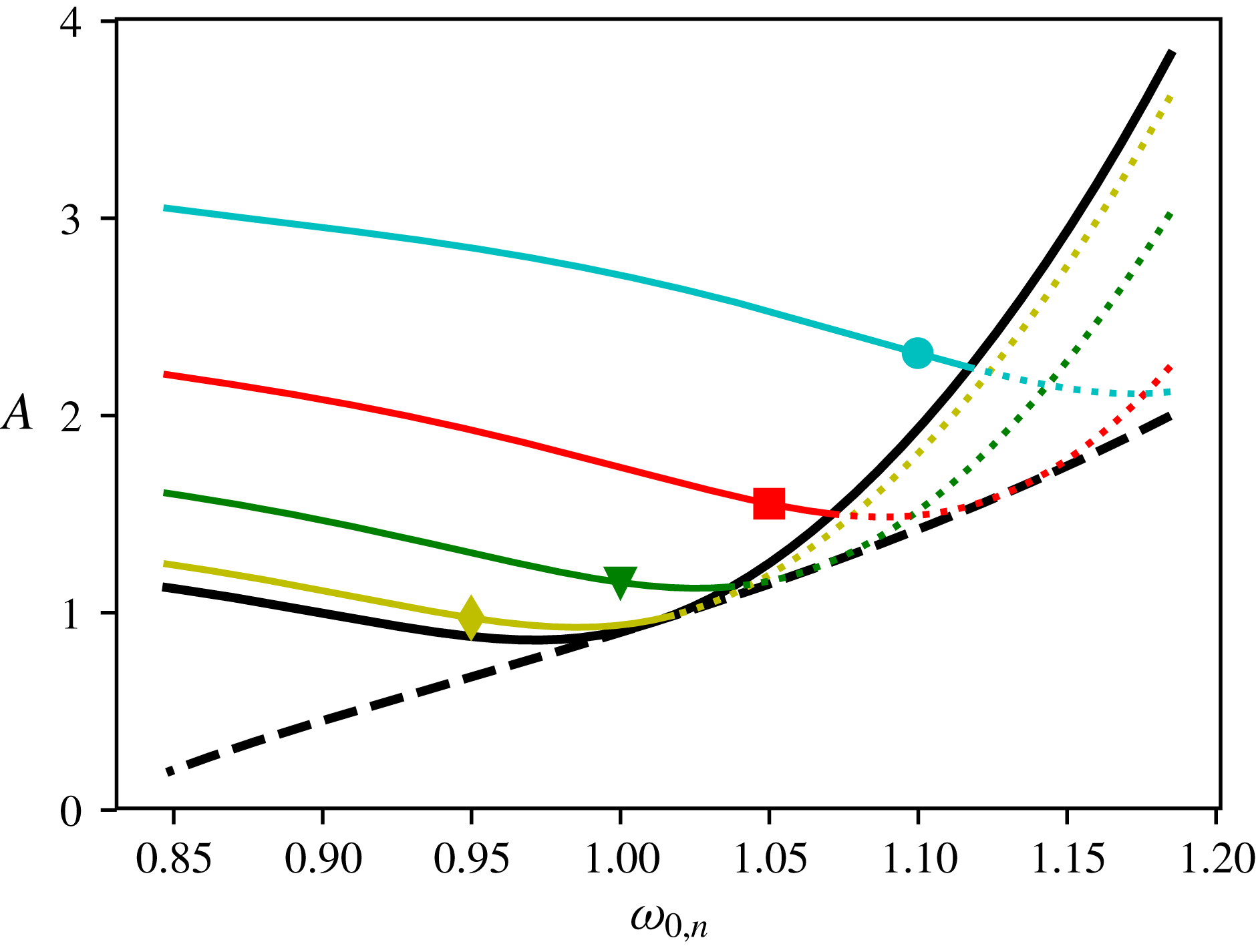
When accounting for nonlinear interaction terms, solving (4.8) and (4.9) allows us to determine the steady-state solutions above the threshold. It is worth noting that (4.8) directly provides the value of applied pressure amplitude
 $A$
to get a given amplitude
 $S_{n}$
of the parametrically forced shape mode
 $n$
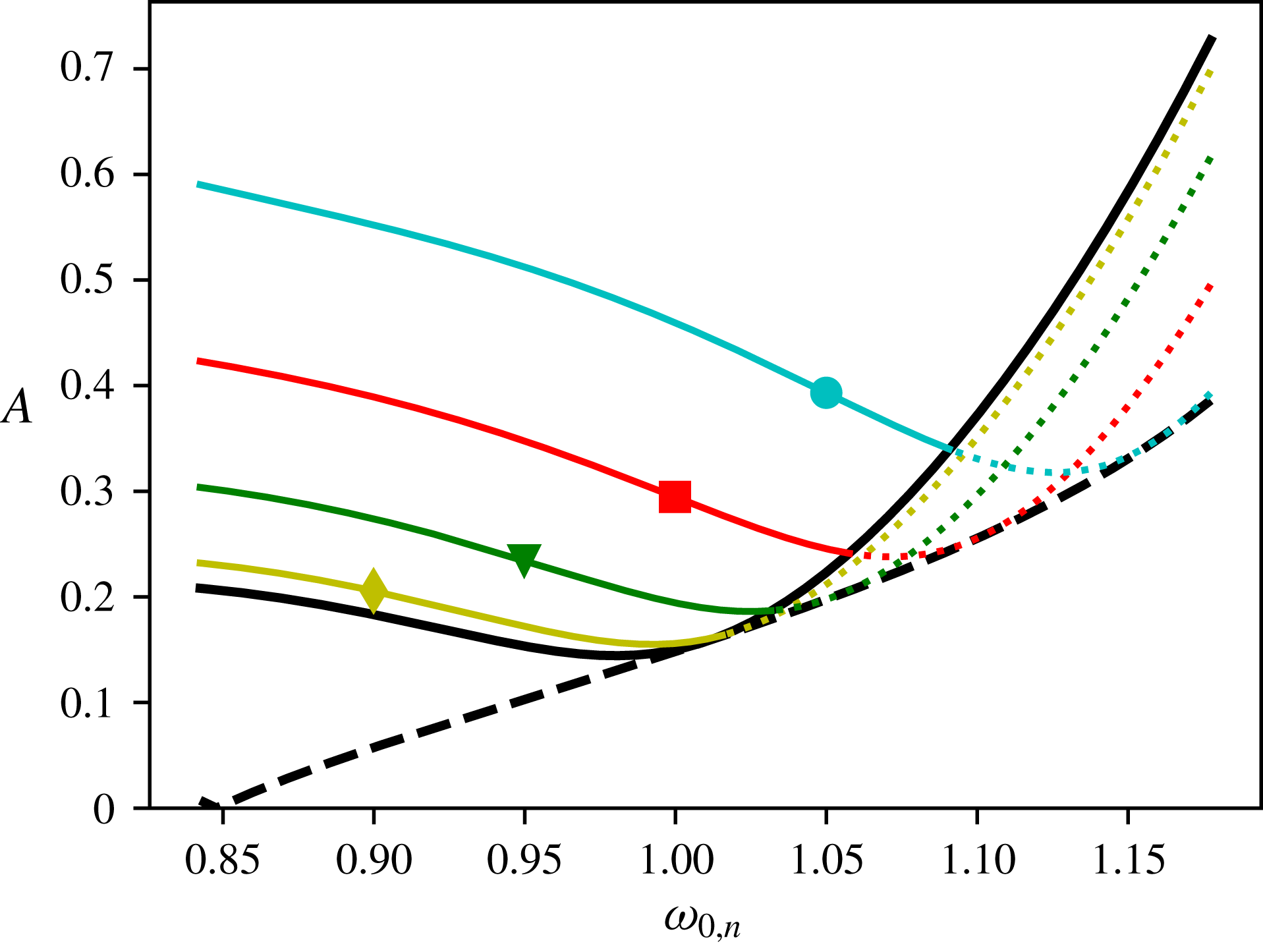
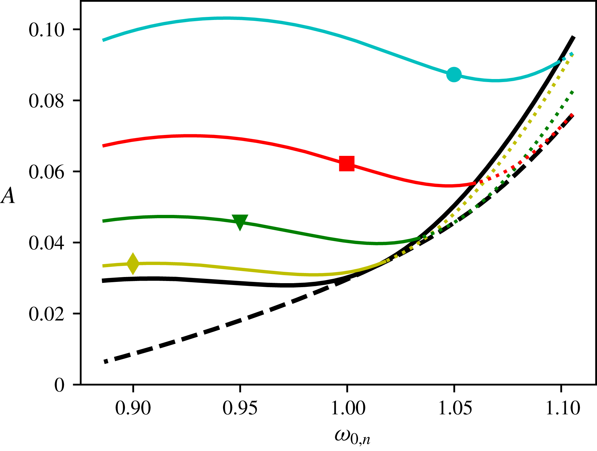
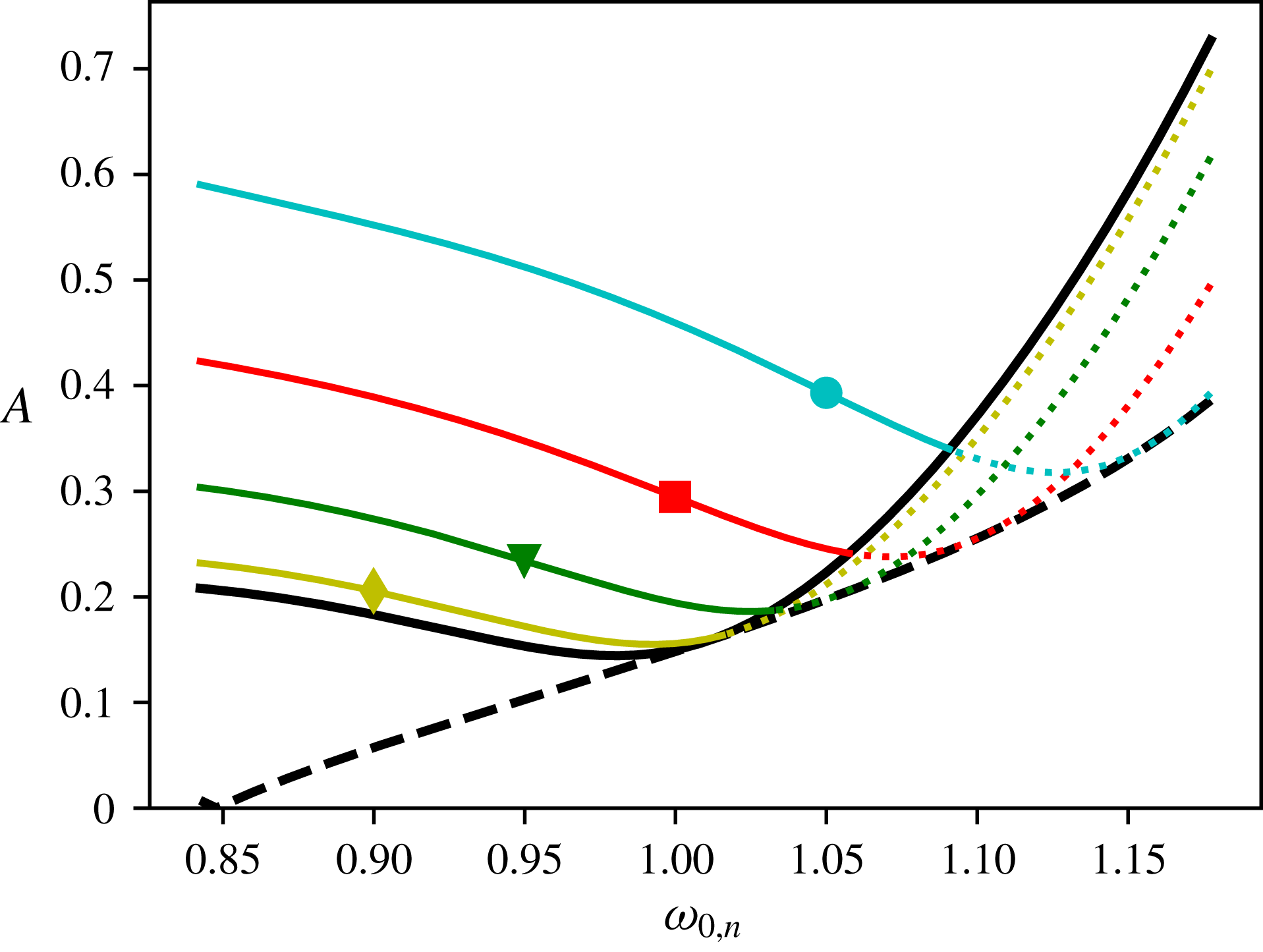
. This is illustrated in figures 5–7 which give the stability areas of the three first shape modes
 $n=2$
,
 $n=3$
and
 $n=4$
, respectively, in the vicinity of the first parametric resonance. The onset threshold curves computed from (4.13) are given by the thick black curves. In each figure, the driving amplitude curves corresponding to isovalues of the shape mode amplitude
 $S_{n}$
(
 $S_{n}=0.1,0.2,0.3,0.4$
) and computed from (4.8) are labelled with different symbols.
Same as figure 5, for
 $n=3$
.
Same as figure 5, for
 $n=4$
.
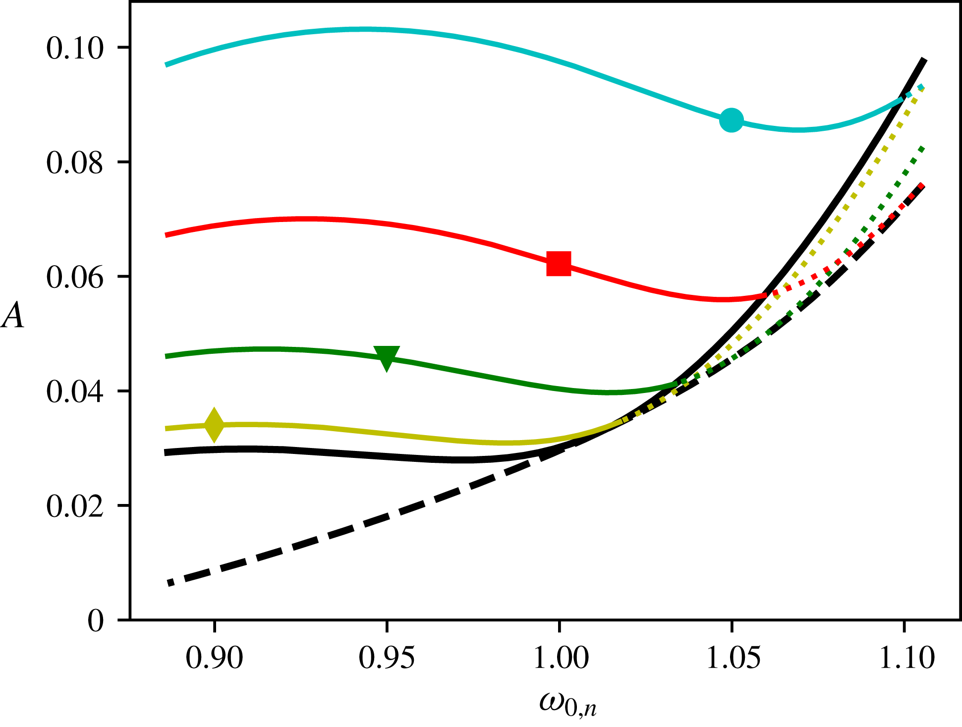
These results enable us to illustrate an important feature of the steady-state solutions, namely that the amplitude curves for a finite value of shape mode amplitude cross the onset threshold curve at particular frequencies. This has two major consequences on the sustained shape oscillations above parametric threshold. First, it indicates that increasing the acoustic driving amplitude to exceed the onset threshold in the region where curves are crossing leads to a jump of the shape mode amplitude from a zero value to a finite non-zero value. Second, one can notice that this region where such a jump is appearing always corresponds to values
 $\unicode[STIX]{x1D714}_{0,n}>1$
, namely for bubble static radii below the parametric resonance radius. It means that for a bubble of static radius smaller than the parametric resonance radius, shape modes suddenly appear with a sharp transition at the onset threshold when increasing the acoustic pressure amplitude. Conversely, shape modes appear with a smooth transition at threshold for a bubble of static radius larger than the parametric resonance radius.
Let us now look at the steady-state solutions of (4.8) which can be expressed as:
 $$\begin{eqnarray}S_{n}=\frac{\sqrt{2g_{0}}}{h_{2}}\left(1\pm \sqrt{1+\frac{h_{2}^{2}(h_{3}A-h_{1})(h_{3}A+h_{1})}{g_{0}^{2}}}\right)^{1/2},\end{eqnarray}$$
where
 $h_{i}=|\bar{h}_{i}|$
and
 $$\begin{eqnarray}g_{0}=\text{Re}(\bar{h}_{1})\text{Re}(\bar{h}_{2})+\text{Im}(\bar{h}_{1})\text{Im}(\bar{h}_{2}).\end{eqnarray}$$
The first requirement for these solutions to be real is that
 $$\begin{eqnarray}A>A_{th}^{\prime }=\frac{1}{h_{3}}\sqrt{(h_{1}-g_{0}/h_{2})(h_{1}+g_{0}/h_{2})},\end{eqnarray}$$
which gives the transition curve between spherically stable and conditionally stable regions. This threshold is represented by thick dashed curves in figures 5–7.
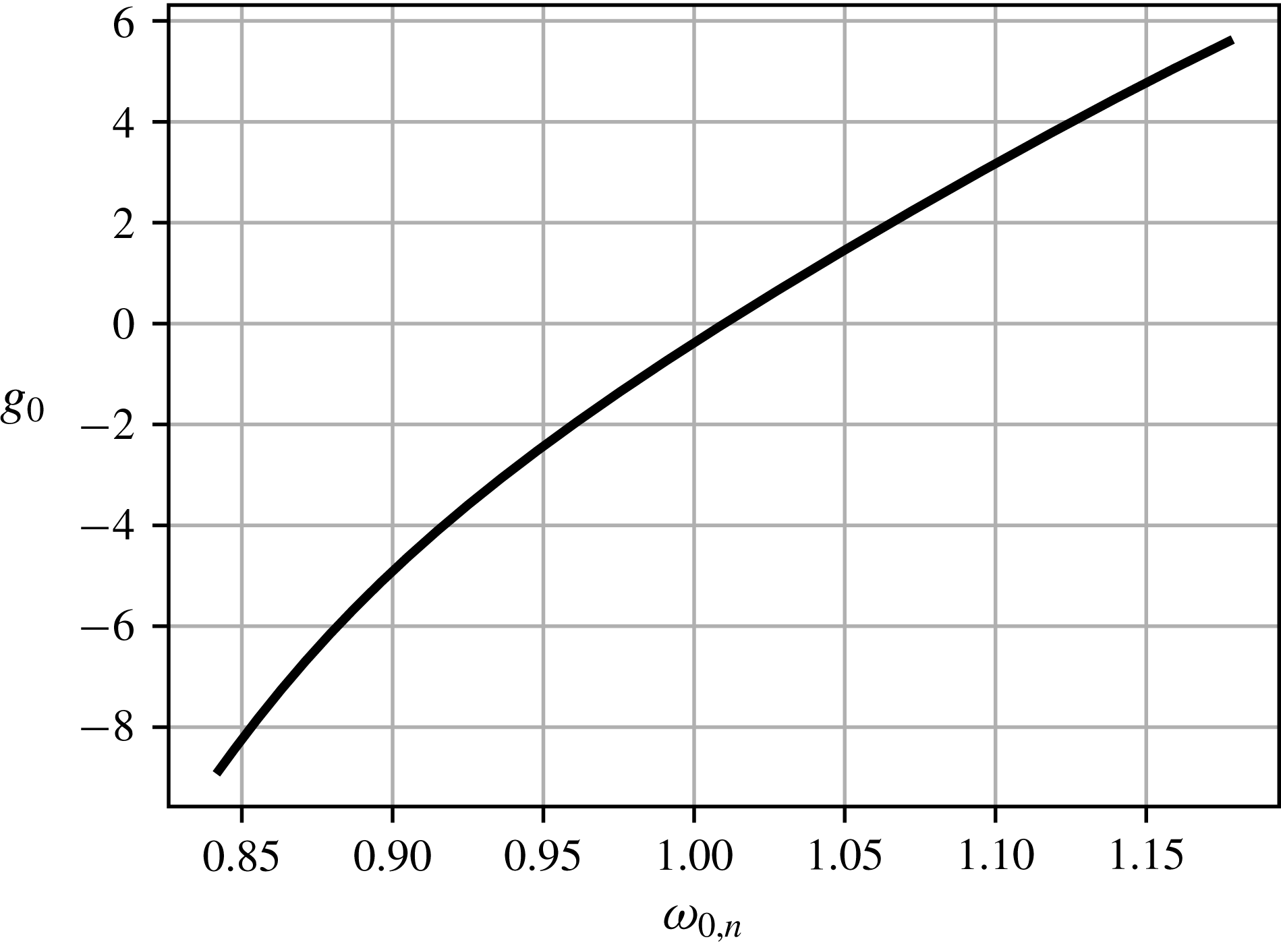
Amplitude-independent quantity
 $g_{0}$
as a function of the frequency
 $\unicode[STIX]{x1D714}_{0,n}$
, here for
 $n=3$
. Note that
 $g_{0}=0$
for
 $\unicode[STIX]{x1D714}_{0,n}=\unicode[STIX]{x1D6FA}^{\ast }\simeq 1$
.
The second requirement to get real steady-state solutions is that
 $$\begin{eqnarray}g_{0}\left(1\pm \sqrt{1+\frac{h_{2}^{2}(h_{3}A-h_{1})(h_{3}A+h_{1})}{g_{0}^{2}}}\right)>0,\end{eqnarray}$$
which depends both on the sign of
 $g_{0}$
and on the sign of the two branches.
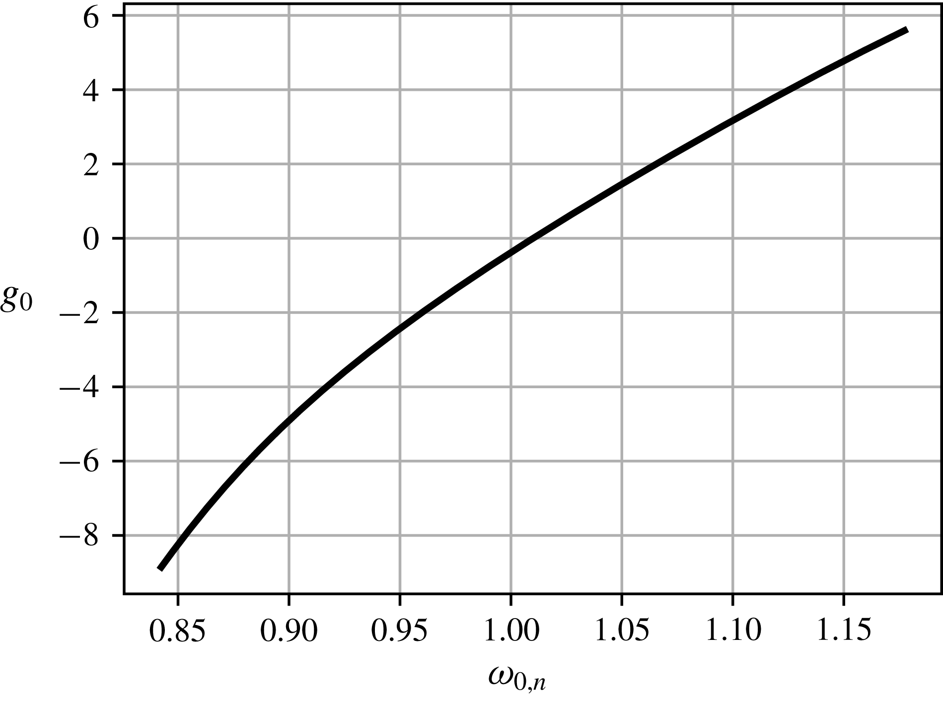
 $g_{0}$
is a frequency-dependent quantity which cancels for
 $\unicode[STIX]{x1D714}_{0,n}=\unicode[STIX]{x1D6FA}^{\ast }\simeq 1$
, and would equal
 $1$
when neglecting viscous effects. From a graphical observation of
 $g_{0}$
, as shown in figure 8, it directly comes that
 $g_{0}>0$
when
 $\unicode[STIX]{x1D714}_{0,n}>\unicode[STIX]{x1D6FA}^{\ast }$
while
 $g_{0}<0$
when
 $\unicode[STIX]{x1D714}_{0,n}<\unicode[STIX]{x1D6FA}^{\ast }$
. Also note that for
 $\unicode[STIX]{x1D714}_{0,n}=\unicode[STIX]{x1D6FA}^{\ast }$
, setting
 $g_{0}=0$
in (4.17) leads to
 $A_{th}^{\prime }=A_{th}$
. This corresponds to the meeting points of the two transition curves in figures 5–7. On the other hand, as soon as the amplitude
 $A$
fulfils the condition (4.17), the upper branch is always positive, while the lower one is conditionally positive, namely if
 $$\begin{eqnarray}1-\sqrt{1+\frac{h_{2}^{2}(h_{3}A-h_{1})(h_{3}A+h_{1})}{g_{0}^{2}}}>0.\end{eqnarray}$$
Because
 $h_{i}$
and
 $g_{0}^{2}$
are all positive quantities, equation (4.19) is only fulfilled if
 $$\begin{eqnarray}A>\frac{h_{1}}{h_{3}},\end{eqnarray}$$
which naturally corresponds to the absolute stability threshold defined by (4.13). The conditions for real steady-state solutions are summarised as follows:
(i) If the driving amplitude is below the conditional stability threshold defined by (4.17), thus both branches are complex and the only possible solution is the trivial one, i.e.
 $S_{n}=0$
.
(ii) If the driving amplitude lies between the boundaries
(4.21)then both solutions are real only if$$\begin{eqnarray}\frac{1}{h_{3}}\sqrt{(h_{1}-g_{0}/h_{2})(h_{1}+g_{0}/h_{2})}<A<\frac{h_{1}}{h_{3}},\end{eqnarray}$$
$g_{0}>0$
(
$\unicode[STIX]{x1D714}_{0,n}>\unicode[STIX]{x1D6FA}^{\ast }$
). In that case, the upper branch is stable while the lower one is unstable.(iii) If the driving amplitude exceeds the absolute stability threshold defined by (4.13), then the upper branch is the only real solution when
$g_{0}>0$
, while the lower one is the only real solution when
$g_{0}<0$
.


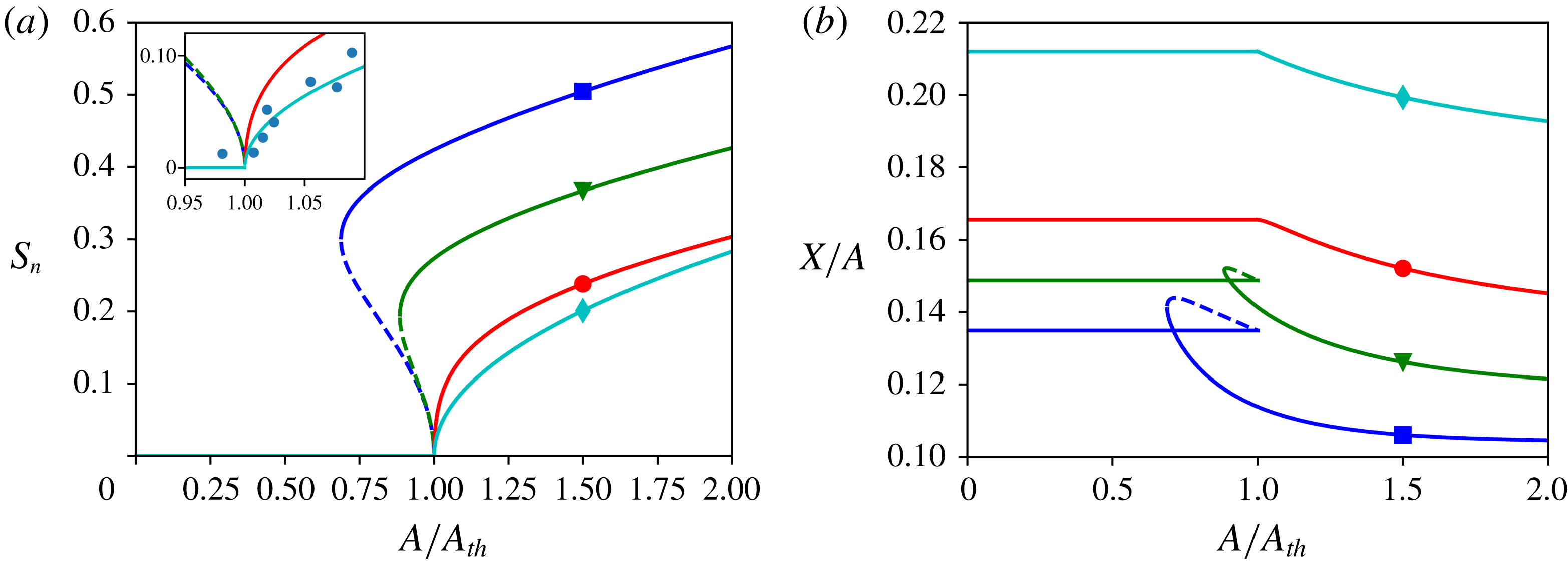
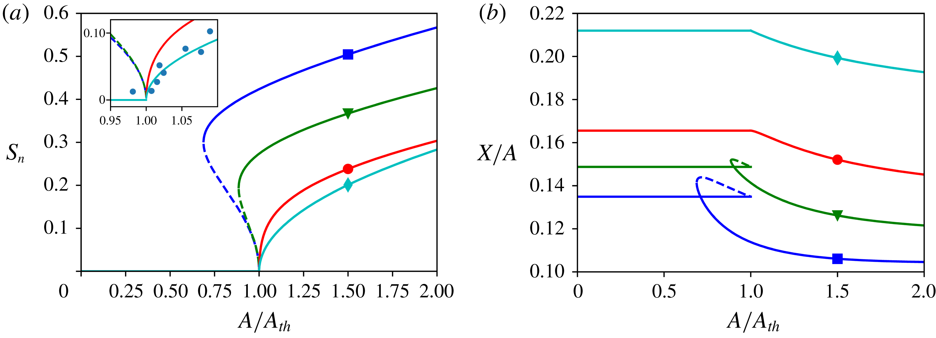
Amplitude of the parametrically forced shape mode (a) and the spherical mode (b) in steady state as a function of the driving amplitude, here for
 $n=3$
. The driving amplitude is divided by the amplitude threshold. Straight (respectively dashed) lines indicate stable (respectively unstable) solutions. The different curves correspond to different frequency values:
 $\unicode[STIX]{x1D714}_{0,n}=0.9$
(♢,
 $g_{0}<0$
),
 $1$
(○,
 $g_{0}<0$
),
 $1.05$
(▿,
 $g_{0}>0$
) and
 $1.1$
(▫,
 $g_{0}>0$
). In (b) the amplitude of the spherical mode is divided by the driving amplitude. The inset graph in (a) shows the curves in the close vicinity of the parametric threshold and a comparison with experimental values (●) that can be found in the work of Guédra et al. (Reference Guédra, Cleve, Mauger, Blanc-Benon and Inserra2017) with
 $R_{0}\simeq 73~\unicode[STIX]{x03BC}\text{m}$
and
 $\unicode[STIX]{x1D714}_{0,3}\simeq 0.87$
.
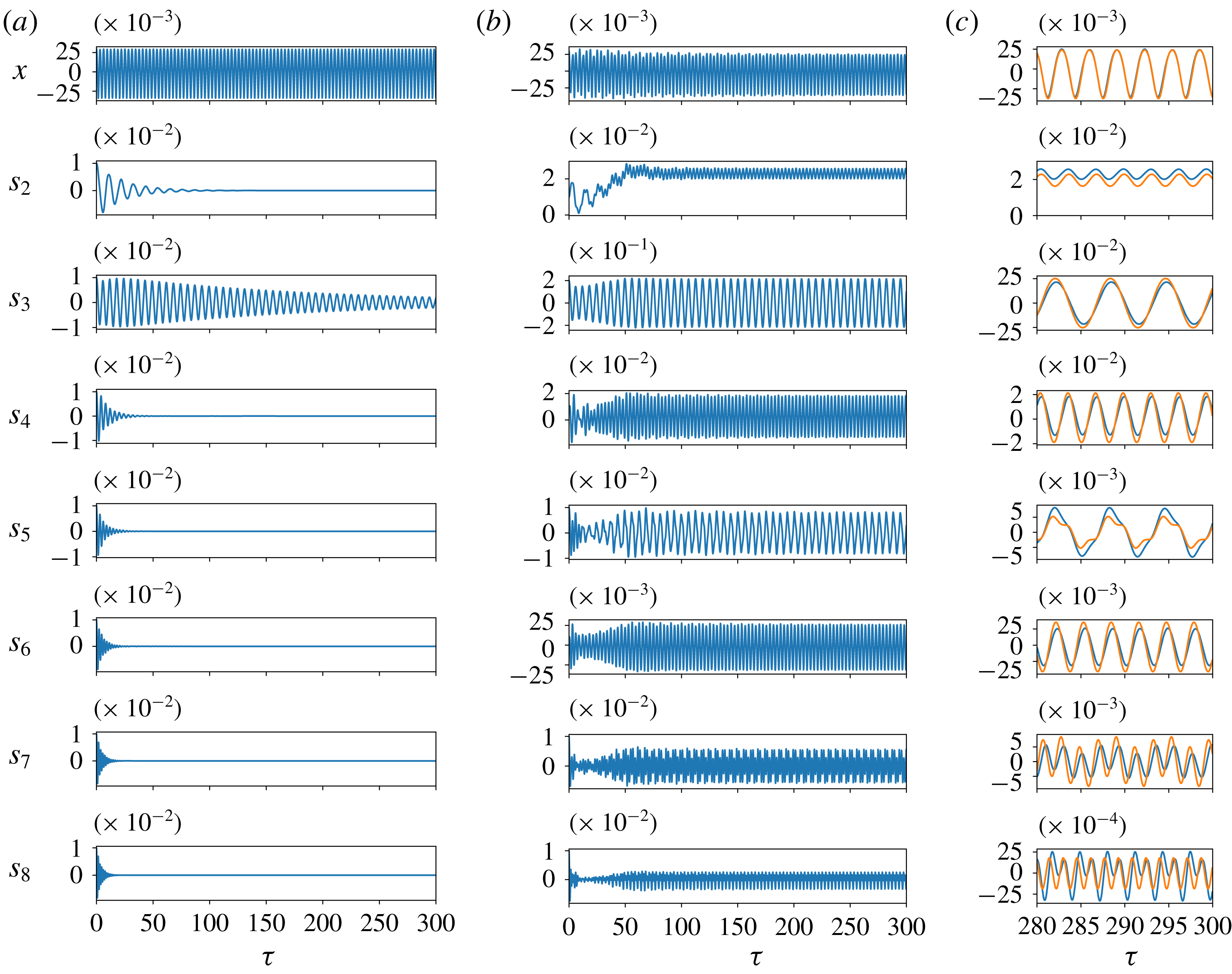
Oscillations of the spherical mode and the seven first shape modes for
 $n=3$
,
 $\unicode[STIX]{x1D714}_{0,n}=1.05$
and
 $A/A_{th}=0.95$
, corresponding to the green ▿ curve shown in figure 9. (a,b) Present numerical simulations obtained from two different initial conditions on the parametrically forced shape mode,
 $s_{3}(0)=10^{-2}$
(a) and
 $s_{3}(0)=0.2$
(b), illustrating the hysteretic behaviour in the region bounded by the conditional threshold and the absolute threshold. (c) Focuses on few acoustic periods during the steady state obtained for the second initial condition, providing a comparison between numerical simulations (blue curves) and first-order approximate solutions (orange curves).

An illustration of these stability conditions is provided in figure 9(a), which gives the steady-state solutions (4.15) as a function of the driving amplitude. The solutions are given here for the
 $n=3$
shape mode. Among the four curves, two of them correspond to
 $\unicode[STIX]{x1D714}_{0,n}=0.9$
and
 $\unicode[STIX]{x1D714}_{0,n}=1$
, so that
 $\unicode[STIX]{x1D714}_{0,n}<\unicode[STIX]{x1D6FA}^{\ast }$
thus
 $g_{0}<0$
. In this case, the only non-zero stable solution is obtained when
 $A>A_{th}$
, and the transition from spherically stable oscillations to non-spherically stable oscillations is continuous. Indeed, it is easy to see that the real lower branch defined by (4.15) leads to
 $S_{n}=0$
when
 $A=A_{th}$
. The two other curves correspond to
 $\unicode[STIX]{x1D714}_{0,n}=1.05$
and
 $\unicode[STIX]{x1D714}_{0,n}=1.1$
, so that
 $\unicode[STIX]{x1D714}_{0,n}>\unicode[STIX]{x1D6FA}^{\ast }$
thus
 $g_{0}>0$
. In this case, a region lies between the boundaries
 $A_{th}^{\prime }$
and
 $A_{th}$
where the spherical and non-spherical oscillations are conditionally stable. A sharp transition exists between the two oscillating regimes, and the real upper branch defined by (4.15) leads to
 $S_{n}=\sqrt{2g_{0}}/h_{2}$
for
 $A=A_{th}^{\prime }$
and
 $S_{n}=2\sqrt{g_{0}}/h_{2}$
for
 $A=A_{th}$
. The stability of both the trivial solution and the upper branch solution in this region leads to an hysteretic behaviour which indicates that stable non-spherical oscillations can be reached even for driving amplitudes below the absolute parametric threshold. To illustrate this, we report in figure 10 two direct numerical simulations of (2.2) and (2.3) corresponding to the green
 $\triangledown$
curve conditions shown in figure 9 and for a driving amplitude
 $A/A_{th}=0.95$
. The two numerical solutions are obtained for two different initial conditions on the
 $n=3$
shape mode. It demonstrates that two different steady states can be reached depending on the initial conditions, namely stable spherical oscillations (figure 10
a), corresponding to the damping of all shape modes (trivial solution
 $S_{n}=S_{m}=0$
), and sustained shape oscillations (figure 10
b) corresponding to the upper branch shown in figure 9. In figure 10(c) is shown a comparison between the numerical solution and the first-order approximate solution in the steady-state regime, proving the consistency of the perturbation method to reproduce the complex structure of the nonlinear coupled oscillations.
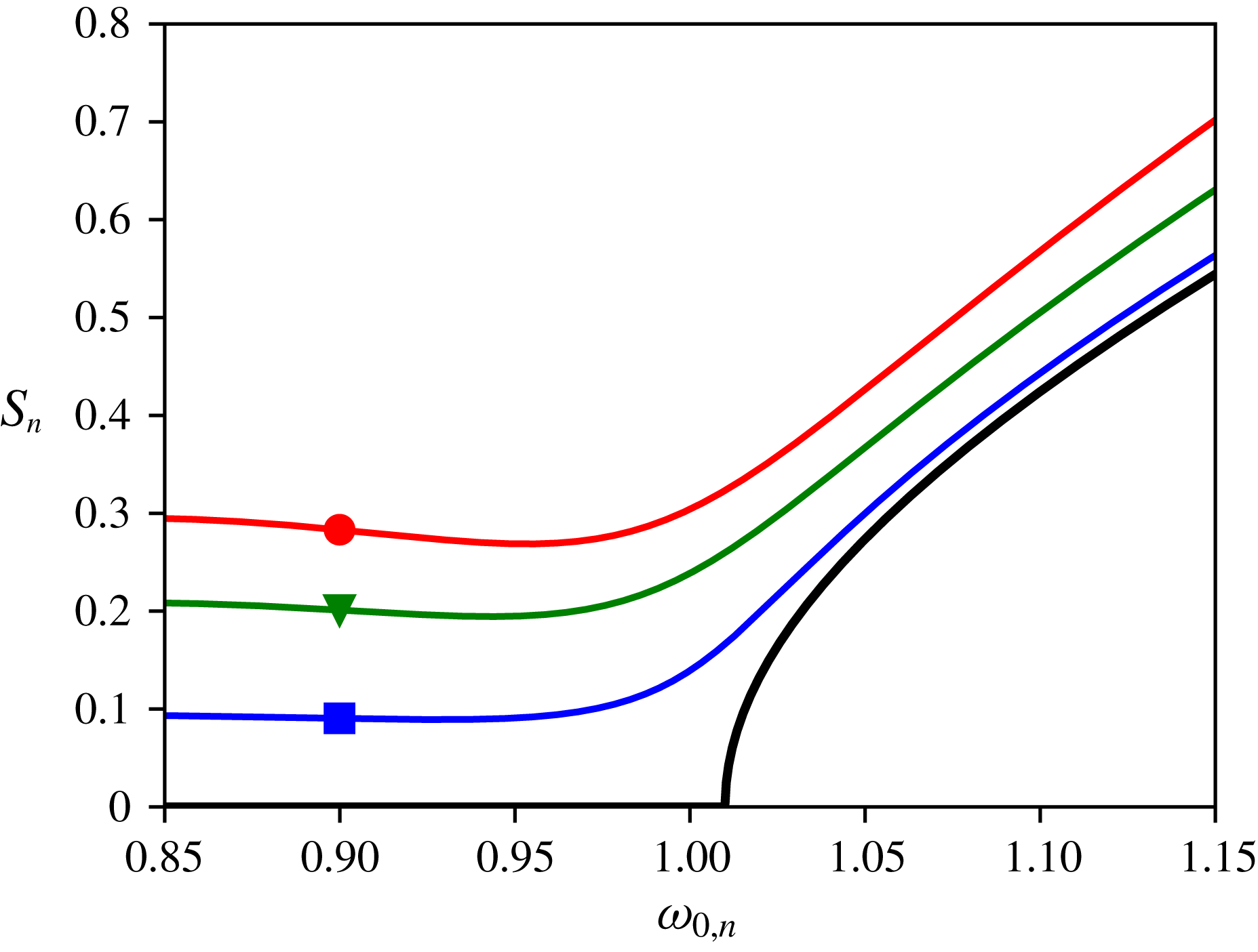
Amplitude of the parametrically forced shape mode
 $S_{n}$
in steady state as a function of the frequency
 $\unicode[STIX]{x1D714}_{0,n}$
, for
 $n=3$
. The thick black curve represents the amplitude at the absolute threshold, namely
 $S_{n}=0$
for
 $g_{0}<0$
and
 $S_{n}=2\sqrt{g_{0}}/h_{2}$
for
 $g_{0}>0$
. The other curves correspond to different driving amplitude ratios above threshold:
 $A/A_{th}=1.1$
(▫),
 $1.5$
(▿) and
 $2$
(○).

Oscillations of the shape mode
 $n$
with the complex amplitude
 $\bar{S}_{n}$
also imply a change in the amplitude of the spherical mode which is mathematically made explicit by (4.5). Figure 9(b) shows the corresponding amplitude of the spherical oscillations in steady state as a function of the driving amplitude, for the same conditions as in the left part. The ratio
 $X/A$
is plotted, so that for driving amplitudes below the absolute threshold (i.e. no shape oscillations,
 $S_{n}=0$
) the linear relationship between the spherical response of the bubble and the external pressure naturally leads to the constant value
 $1/|\bar{\unicode[STIX]{x1D6E5}}_{0}|$
. However sustained shape oscillations of finite amplitude lead to a global decrease of the amplitude of the spherical mode. This is clearly observed in figure 9 and can be also noticed on the temporal solutions shown in figures 1–3. For the same reasons as mentioned previously, an hysteretic loop is also obtained when
 $\unicode[STIX]{x1D714}_{0,n}>\unicode[STIX]{x1D6FA}^{\ast }$
for driving amplitudes bounded by the conditional stability and absolute stability thresholds.
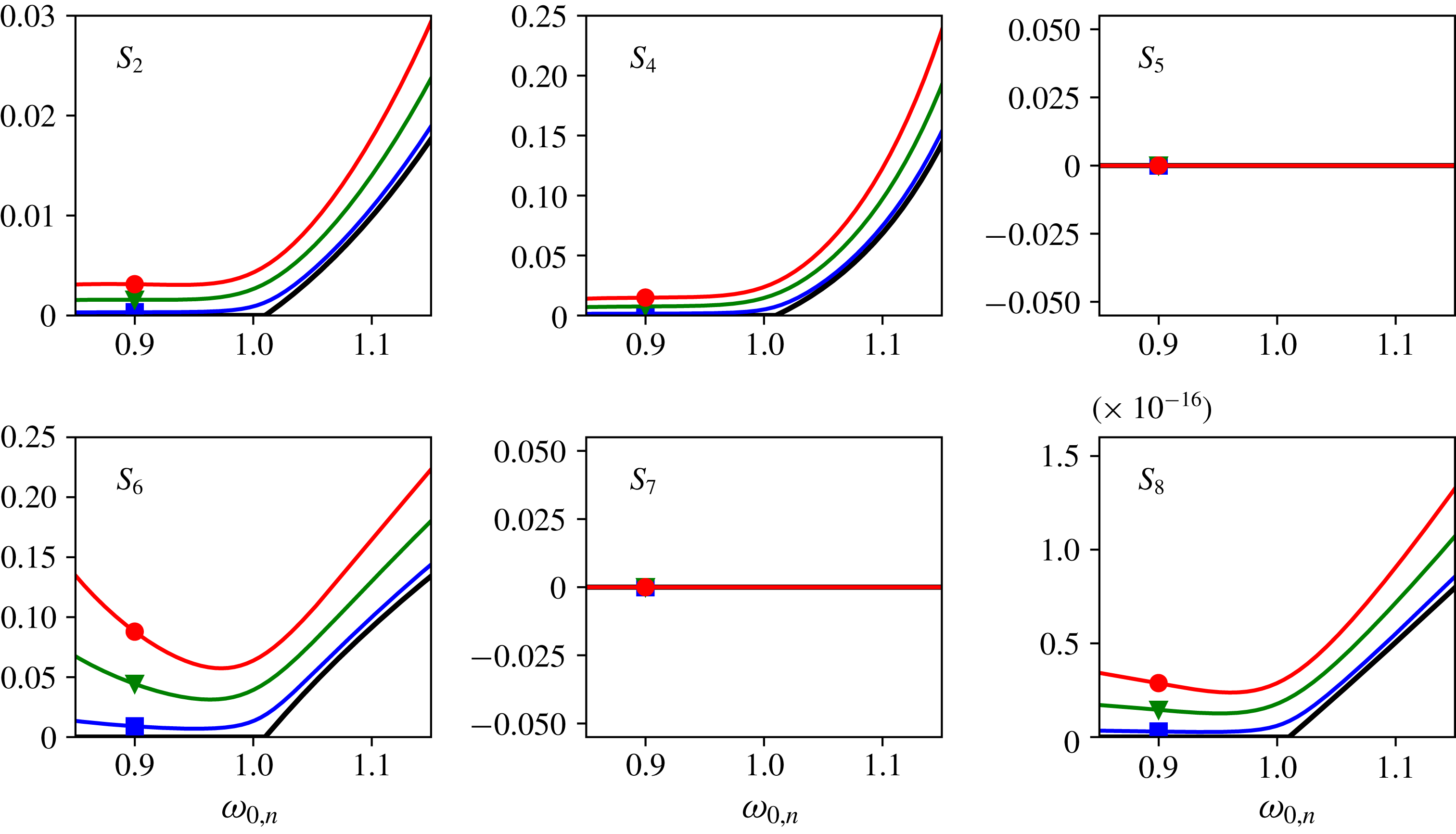
Amplitude of the secondary shape modes
 $S_{m}$
in steady state as a function of the frequency
 $\unicode[STIX]{x1D714}_{0,n}$
, for
 $n=3$
. See the caption of figure 11 for the legend.

As the final point of the discussion, we recall that in the framework of the present analysis, the saturation of the parametrically forced shape mode
 $n$
can only come from nonlinear interactions involving secondary shape modes
 $m\neq n$
. As soon as the amplitude of the shape mode
 $n$
in steady state is determined, the amplitudes of all the secondary modes are directly deduced from (4.6). The figures 11 and 12 show the variations of the shape mode amplitudes in the vicinity of the first parametric resonance of the
 $n=3$
mode, for different values of the driving amplitude at and above the absolute threshold. The threshold curves (
 $A=A_{th}$
, thick black curves) remind us that
 $S_{n}=0$
is the only stable solution for
 $\unicode[STIX]{x1D714}_{0,n}<\unicode[STIX]{x1D6FA}^{\ast }$
, while
 $S_{n}\neq 0$
at threshold for
 $\unicode[STIX]{x1D714}_{0,n}>\unicode[STIX]{x1D6FA}^{\ast }$
. The figure 12 also reveals that secondary odd shape modes have vanishing amplitudes at the lowest order (
 $S_{5}=S_{7}=0$
), while these modes are after all excited through nonlinear coupling as illustrated in figures 2 or 10. First, this means that only even modes participate to the nonlinear saturation of the parametrically excited shape mode (
 $n=3$
) at the lowest order. Second, it implies that oscillations of additional odd modes thus only appear at first order, following solution (3.10), which explains why these modes mainly oscillate at the frequencies
 $\unicode[STIX]{x1D70F}$
or
 $3\unicode[STIX]{x1D70F}$
rather than at the driving frequency
 $2\unicode[STIX]{x1D70F}$
. This is clearly observed on the temporal solutions for
 $s_{5}$
and
 $s_{7}$
given in figures 2 and 10. It is interesting to note that the perturbation analysis allows us to capture this specific behaviour although it goes beyond the validity framework of the asymptotic approach expressed by (3.6).
5 Conclusion
Bubble shape oscillations of finite amplitude have been analysed using a perturbation method based on the Krylov–Bogoliubov asymptotic technique. Nonlinear interactions between spherical and non-spherical modes in the coupled fluid dynamical equations have been shown to induce the saturation of the parametric instability. This nonlinear saturation allowed the shape oscillations to reach a steady state. An analysis of the solutions in the permanent regime revealed that shape oscillations can be conditionally stable below the classical parametric threshold. It demonstrated that an hysteretic behaviour can be obtained since both spherical and non-spherical oscillations can be stable in a region bounded by the conditional stability threshold and the absolute stability (parametric) threshold. This hysteresis is naturally accompanied by a sharp transition (a ‘jump’) between spherically stable oscillations and shape oscillations when crossing the threshold. The present analysis also proved that this sharp transition is only obtained for frequencies larger than the parametric resonance condition, i.e. for bubbles of static radius smaller than the parametric resonance radius. On the other hand, considering bubbles of static radius larger than the parametric resonance radius, the parametric threshold is characterised by a smooth transition between spherically stable oscillations and shape oscillations, whose amplitude is vanishing at the transition curve. By conducting the derivations accounting for nonlinear mode coupling without restriction on the number of shape modes, we also showed that only even modes participate in the saturation of the main parametrically forced mode at the second order of approximation. Hence, additional odd modes coming from nonlinear coupling only involve oscillations at the first order, thus explaining why they mainly oscillate at harmonic or subharmonic frequencies rather than at the driving frequency (twice the parametric resonance frequency). Finally, we must recall that the current equations are derived in the vicinity of the first parametric resonance of the main unstable shape mode (
 $\unicode[STIX]{x1D714}\simeq 2\unicode[STIX]{x1D6FA}_{n}$
) and considering weakly nonlinear spherical oscillations far from their primary and harmonic resonances. Appropriate changes should be made on the zero-order solutions and on the identification of corresponding secular terms to account for other resonant conditions.
Acknowledgements
This work was supported by the French National Research Agency ANR-MOST project CARIBBBOU (ANR-15-CE19-0003) and the LabEx CeLyA of the University of Lyon (ANR-10-LABX-0060/ANR-11-IDEX-0007).
Appendix A. Nonlinear interaction coefficients
Introducing the variable
 $\unicode[STIX]{x1D707}=\cos \unicode[STIX]{x1D703}$
, the following quantities are defined:
 $$\begin{eqnarray}\displaystyle & \displaystyle I_{a_{nij}}=\int _{-1}^{1}P_{n}P_{i}P_{j}\,\text{d}\unicode[STIX]{x1D707}, & \displaystyle\end{eqnarray}$$
 $$\begin{eqnarray}\displaystyle & \displaystyle I_{c_{nij}}=\int _{-1}^{1}(1-\unicode[STIX]{x1D707}^{2})P_{n}\frac{\text{d}P_{i}}{\text{d}\unicode[STIX]{x1D707}}\,\frac{\text{d}P_{j}}{\text{d}\unicode[STIX]{x1D707}}\,\text{d}\unicode[STIX]{x1D707}, & \displaystyle\end{eqnarray}$$
 $$\begin{eqnarray}\displaystyle & \displaystyle G_{e_{nij}}=\frac{[n(n-j)+3(j+1)]I_{a_{nij}}+I_{c_{nji}}}{(n+1)(j+1)}, & \displaystyle\end{eqnarray}$$
 $$\begin{eqnarray}\displaystyle & \displaystyle M_{c_{nij}}=G_{e_{nij}}+G_{e_{jin}}, & \displaystyle\end{eqnarray}$$
 $$\begin{eqnarray}\displaystyle & \displaystyle M_{d_{nij}}=G_{e_{nij}}+G_{e_{jin}}-G_{e_{inj}}, & \displaystyle\end{eqnarray}$$
 $$\begin{eqnarray}\displaystyle & \displaystyle J_{a_{nij}}=4WI_{a_{nij}}+\unicode[STIX]{x1D714}_{0,j}^{2}M_{c_{nij}}. & \displaystyle\end{eqnarray}$$
The coefficients appearing in the first-order differential equations (3.7a–f ) and in the first-order solutions (3.8)–(3.10) are given by:
 $$\begin{eqnarray}\displaystyle & \displaystyle \unicode[STIX]{x1D6FC}_{n}=\frac{(n+3)\unicode[STIX]{x1D714}_{0,n}^{2}-(n+1)\unicode[STIX]{x1D714}_{0}^{2}-\displaystyle (n+{\textstyle \frac{3}{2}})(\dot{\unicode[STIX]{x1D703}}_{n})^{2}}{(2n+1)(n+1)}, & \displaystyle\end{eqnarray}$$
 $$\begin{eqnarray}\displaystyle & \displaystyle \unicode[STIX]{x1D6FD}_{n}=\frac{(n+3)\unicode[STIX]{x1D714}_{0,n}^{2}-(n+1)\unicode[STIX]{x1D714}_{0}^{2}+\displaystyle (n+{\textstyle \frac{3}{2}})(\dot{\unicode[STIX]{x1D703}}_{n})^{2}}{(2n+1)(n+1)}, & \displaystyle\end{eqnarray}$$
 $$\begin{eqnarray}\displaystyle & \displaystyle \unicode[STIX]{x1D6FE}_{n}=3\unicode[STIX]{x1D714}_{0,n}^{2}-(n-1)\unicode[STIX]{x1D714}_{0}^{2}-3\dot{\unicode[STIX]{x1D703}}_{x}\dot{\unicode[STIX]{x1D703}}_{n}, & \displaystyle\end{eqnarray}$$
 $$\begin{eqnarray}\displaystyle & \displaystyle \unicode[STIX]{x1D6FF}_{n}=3\unicode[STIX]{x1D714}_{0,n}^{2}-(n-1)\unicode[STIX]{x1D714}_{0}^{2}+3\dot{\unicode[STIX]{x1D703}}_{x}\dot{\unicode[STIX]{x1D703}}_{n}, & \displaystyle\end{eqnarray}$$
 $$\begin{eqnarray}\displaystyle W_{nm} & = & \displaystyle \frac{(2n+1)(n+1)}{4} (\!W[8I_{a_{nnm}}+(m^{2}-1)(m+2)M_{c_{nnm}}+(n^{2}-1)(n+2)M_{c_{nmn}}\!]\nonumber\\ \displaystyle & & \displaystyle -\,2[M_{d_{nnm}}+M_{d_{nmn}}]\!),\end{eqnarray}$$
 $$\begin{eqnarray}O_{mn}=\frac{(2m+1)(m+1)}{4}(W[4I_{a_{mnn}}+(n^{2}-1)(n+2)M_{c_{mnn}}\!]+M_{d_{mnn}}).\end{eqnarray}$$