1 Introduction
The present study may be viewed as a stepping stone towards the two-dimensional (2-D) inviscid flow solution for an airfoil translating steadily across a uniform-shear approach flow; i.e. where the free stream velocity varies linearly with the cross-stream coordinate. The overall motivation of the work is to understand the basic aerodynamics of wings during aircraft landing in the presence of wind shear. Tsien (Reference Tsien1943) provided the first inviscid flow field and load calculation for a 2-D static Joukowsky airfoil in the presence of uniform free stream shear. In his approach, Tsien first solved the problem of a 2-D static circular cylinder in uniform-shear flow by superposing the stream function of the inviscid approach stream onto a potential disturbance stream function caused by the presence of the cylinder. Subsequently, he utilized conformal mapping of the potential-disturbance solution to solve the static airfoil problem.
Tsien’s work was later extended to more general approach-stream velocity/shear profiles by James (Reference James1951), Honda (Reference Honda1960) and Nishiyama & Hirano (Reference Nishiyama and Hirano1970), among others. Corresponding work for an airfoil traversing across the approach stream could not be found; leading to the present effort. Following Tsien’s approach, we first consider the inviscid 2-D circular cylinder problem before turning our attention to the flow around an airfoil. Since the circular cylinder flow is of general interest by itself, and given that no similar analysis could be found in the literature, the present paper is focused on the cylinder flow. Future work will extend the current results to solve the Joukowsky airfoil problem.
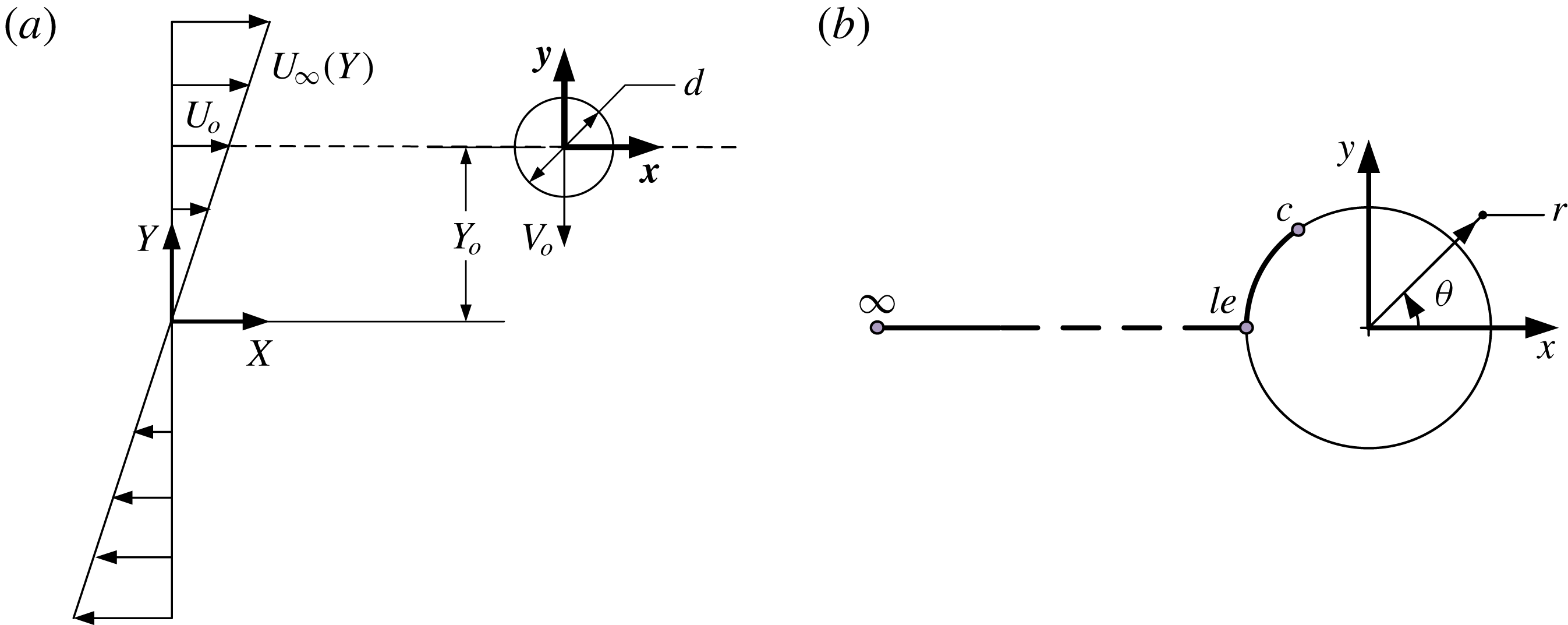
The flow configuration of interest is depicted in figure 1(a). An unbounded stream having uniform positive shear
 $\text{d}U_{\infty }/\text{d}Y=m$
flows over a circular cylinder having a diameter
 $d$
and moving with a constant velocity of magnitude
 $V_{o}$
across the stream in the negative direction. Following Tsien (Reference Tsien1943), a velocity scale is defined as
 $U_{o}$
, which is the velocity of the approach stream at the coordinate of the cylinder’s centre
 $Y_{o}$
. Because of the cylinder’s motion, both
 $Y_{o}$
and
 $U_{o}$
are now time dependent; distinctly different from Tsien’s problem. Two different coordinate systems are employed: X–Y, a ‘laboratory frame’, and x–y, a moving frame attached to the cylinder. The approach stream shear is characterized using the non-dimensional parameter (Tsien Reference Tsien1943),
 $$\begin{eqnarray}\displaystyle & \displaystyle K=\frac{\text{d}U_{\infty }}{\text{d}Y}\frac{d}{U_{o}}. & \displaystyle\end{eqnarray}$$
The shear rate
 $K$
is uniquely set by the non-dimensional coordinate
 $Y_{o}^{\ast }\equiv Y_{o}/(d/2)$
of the cylinder; specifically,
 $$\begin{eqnarray}\displaystyle & \displaystyle K=\frac{md}{U_{o}}=\frac{md}{mY_{o}}=\frac{2}{Y_{o}^{\ast }}. & \displaystyle\end{eqnarray}$$
Equation (1.2) shows that for a static cylinder placed very far (
 $Y_{o}^{\ast }\rightarrow \infty$
) from the shear centre (
 $Y_{o}^{\ast }=0$
and
 $U_{\infty }=0$
),
 $K\rightarrow 0$
and hence the approach flow is effectively uniform. As
 $Y_{o}^{\ast }$
approaches the shear centre (where
 $U_{\infty }=0$
),
 $K$
increases monotonically, reaching an infinite value when
 $Y_{o}^{\ast }=0$
. The infinite
 $K$
magnitude is an outcome of
 $U_{o}=0$
at the centre of shear; the choice of the velocity scale
 $U_{o}$
in defining
 $K$
is taken from Tsien (Reference Tsien1943).
Schematic drawing, coordinate systems and definitions of the moving-cylinder problem: (a) overall problem, (b) details of the coordinate systems fixed to the cylinder. Points
 $\infty$
,
 $le$
and c represent the undisturbed approach stream, the cylinder’s leading edge, and a generic point on the cylinder surface, respectively, on a path used to integrate unsteady Bernoulli’s equation (2.18) in § 2.2.

The objective of the present analysis is to obtain the inviscid flow field streamlines, the surface pressure distribution and the force acting on the cylinder moving across the shear stream. In addition, we address a fundamental question, with important practical ramifications, regarding the connection between the static- and the moving-cylinder flows. More specifically, for any object traversing steadily across a uniform free stream, a Galilean transformation (GT) to the moving object’s frame of reference is traditionally used to deduce the flow field and forces acting on the object from its counterpart when the object is stationary. In the GT frame, the free stream approaches at an effective velocity
 $U_{\infty ,eff}=U_{\infty }\sqrt{1+V_{r}^{2}}$
and incidence angle of
 $\tan ^{-1}(V_{r})$
; where
 $V_{r}$
is the ratio of the object to free stream velocity. In the same vein, we ask the question of whether it remains possible to utilize a GT to connect static- and moving-cylinder flows in the presence of uniform shear in the approach stream.
2 Analysis and results
2.1 Flow field
Tsien (Reference Tsien1943) gives the stream function
 $\unicode[STIX]{x1D713}$
for a static cylinder in uniform-shear flow as
 $$\begin{eqnarray}\displaystyle & \displaystyle \unicode[STIX]{x1D713}=U_{o}\left[\left(r-\frac{d^{2}}{4r}\right)\sin \unicode[STIX]{x1D703}+\frac{K}{2}\left(\frac{r^{2}}{d}\sin ^{2}\unicode[STIX]{x1D703}+\frac{d^{3}}{32r^{2}}\cos 2\unicode[STIX]{x1D703}\right)\right], & \displaystyle\end{eqnarray}$$
where,
 $r$
and
 $\unicode[STIX]{x1D703}$
are polar coordinates (as depicted in figure 1
b) and
 $K$
is the non-dimensional shear rate given by (1.1). Equation (2.1) is the solution of the equation,
 $$\begin{eqnarray}\displaystyle & \displaystyle \unicode[STIX]{x1D6FB}^{2}\unicode[STIX]{x1D713}=\unicode[STIX]{x1D714}_{z}=-\frac{\text{d}U_{\infty }}{\text{d}Y}=-m, & \displaystyle\end{eqnarray}$$
where,
 $\unicode[STIX]{x1D714}_{z}$
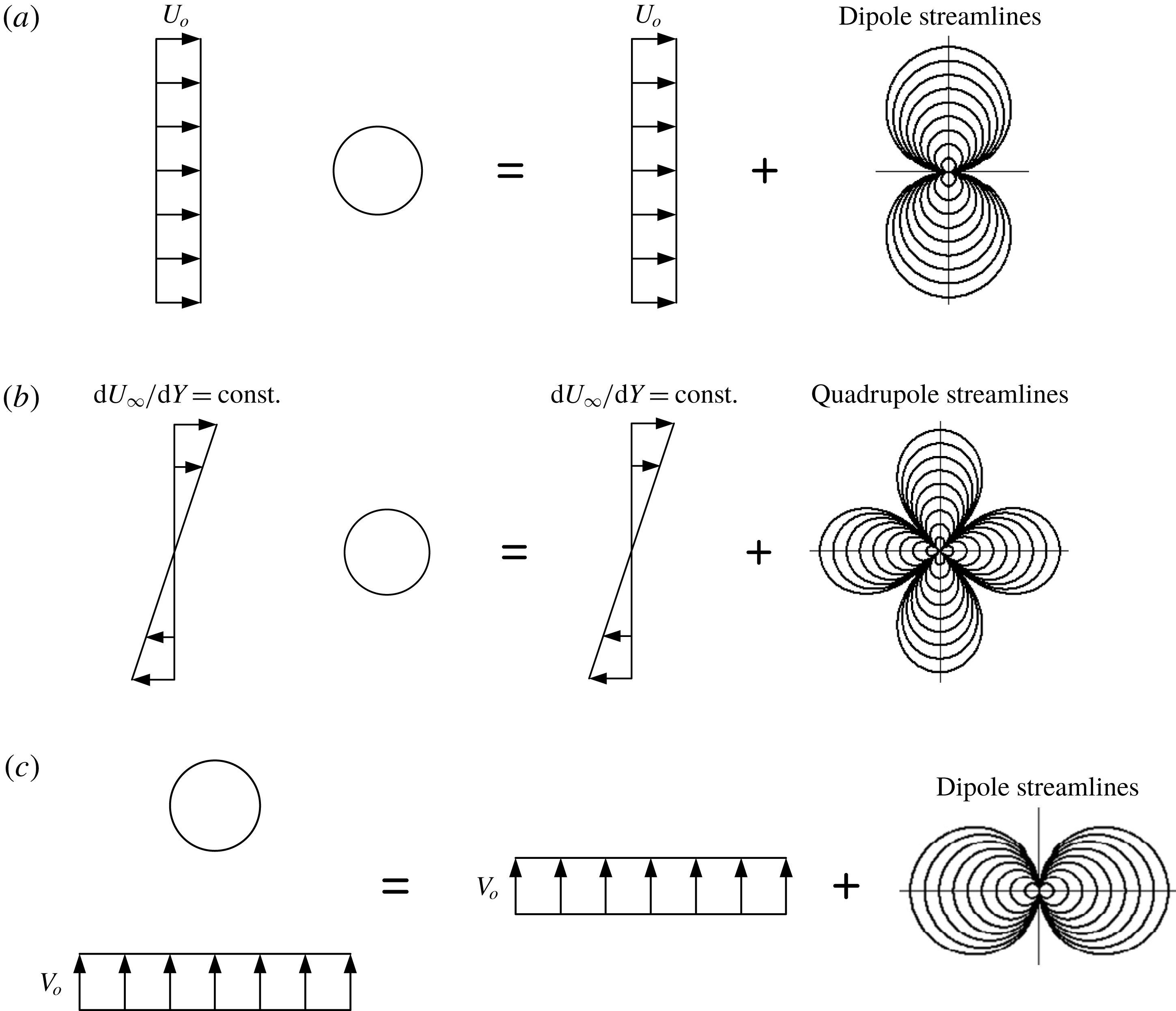
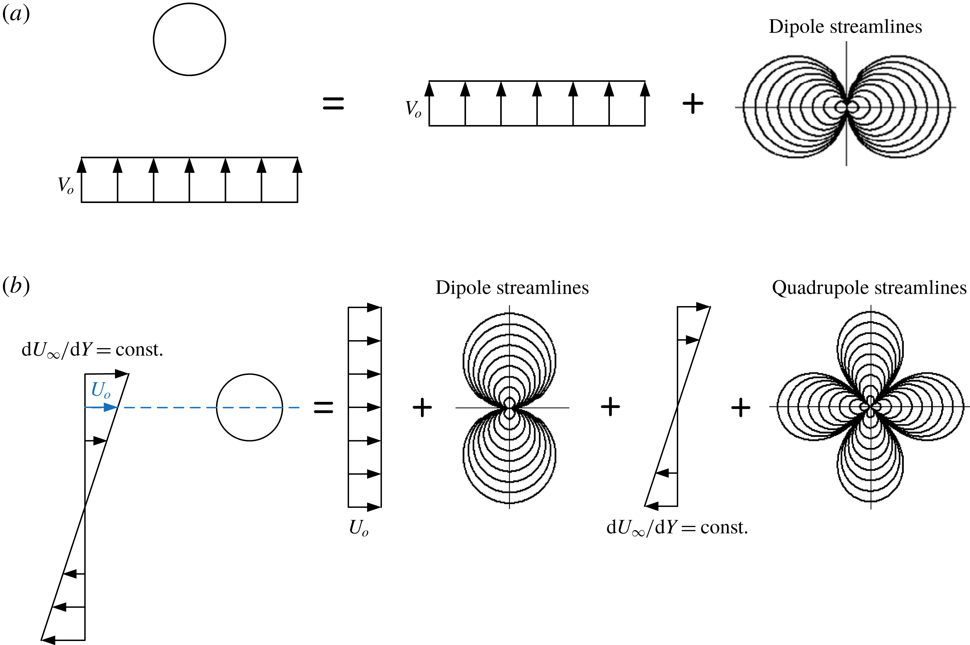
is the uniform out-of-plane vorticity in the approach stream, subject to the boundary conditions of the cylinder surface being a streamline and the disturbance produced by the cylinder decays to zero at infinity. Because (2.2) is linear, (2.1) is arrived at by the superposition of two flow fields. The first is the classical potential flow solution of uniform flow
 $U_{o}$
over a cylinder, which is obtained by the addition of the stream functions of a uniform velocity field and a source dipole (see figure 2
a). The second flow field is that of a ‘centred’ uniform-shear flow over the cylinder (the term ‘centred’ indicates placement of the cylinder at the centre of shear;
 $U_{\infty }=0$
). Based on Tsien’s solution, it can be shown that the latter flow field is equivalent to superposing the stream functions of the centred uniform-shear flow and a source quadrupole (see figure 2
b).
The corresponding velocity components are computed from (2.1) using
 $$\begin{eqnarray}\displaystyle & \displaystyle U_{r}=\frac{1}{r}\frac{\unicode[STIX]{x2202}\unicode[STIX]{x1D713}}{\unicode[STIX]{x2202}\unicode[STIX]{x1D703}}\quad \text{and}\quad U_{\unicode[STIX]{x1D703}}=-\frac{\unicode[STIX]{x2202}\unicode[STIX]{x1D713}}{\unicode[STIX]{x2202}r}, & \displaystyle\end{eqnarray}$$
which leads to
 $$\begin{eqnarray}\displaystyle & \displaystyle \frac{U_{r}}{U_{o}}=U_{r}^{\ast }=\left(1-\frac{1}{r^{\ast 2}}\right)\cos \unicode[STIX]{x1D703}+\frac{K}{2}\left(r^{\ast }\sin \unicode[STIX]{x1D703}\cos \unicode[STIX]{x1D703}-\frac{1}{2r^{\ast 3}}\sin 2\unicode[STIX]{x1D703}\right), & \displaystyle\end{eqnarray}$$
 $$\begin{eqnarray}\displaystyle & \displaystyle \frac{U_{\unicode[STIX]{x1D703}}}{U_{o}}=U_{\unicode[STIX]{x1D703}}^{\ast }=-\left(1+\frac{1}{r^{\ast 2}}\right)\sin \unicode[STIX]{x1D703}-\frac{K}{2}\left(r^{\ast }\sin ^{2}\unicode[STIX]{x1D703}-\frac{1}{2r^{\ast 3}}\cos 2\unicode[STIX]{x1D703}\right), & \displaystyle\end{eqnarray}$$
where, an asterisk denotes non-dimensionalization of all length scales by the cylinder’s radius
 $d/2$
and velocity scales by
 $U_{o}$
.
Superposition of elemental flows leading to: (a) streamwise uniform potential flow around a circular cylinder, (b) ‘centred’ uniform-shear inviscid flow around a circular cylinder (the term ‘centred’ indicates the cylinder is located on the shear centre, where
 $U_{\infty }=0$
) and (c) cross-stream uniform potential flow around a circular cylinder. Superposition of the flows shown in (a) and (b) leads to the stationary cylinder solution of Tsien (Reference Tsien1943). Superposition of the flows shown in (a), (b) and (c) provides the solution for the cylinder traversing steadily across unbounded uniform-shear flow in the GT frame of reference.

To obtain the solution for the moving-cylinder problem, and following Tsien (Reference Tsien1943), we consider the moving cylinder to introduce a potential disturbance to the shear flow (i.e. the only vortical fluid is that associated with the approach stream). The resulting vorticity field is uniform, and hence (2.2) remains linear; i.e. we can superpose different stream functions to obtain the overall solution. Viewing the flow in the moving
 $x{-}y$
frame via a GT, the flow may still be decomposed into the same two components as in the static cylinder case (figures 2
a and 2
b), in addition to a third flow component representing uniform cross-stream flow
 $V_{o}$
relative to the cylinder (figure 2
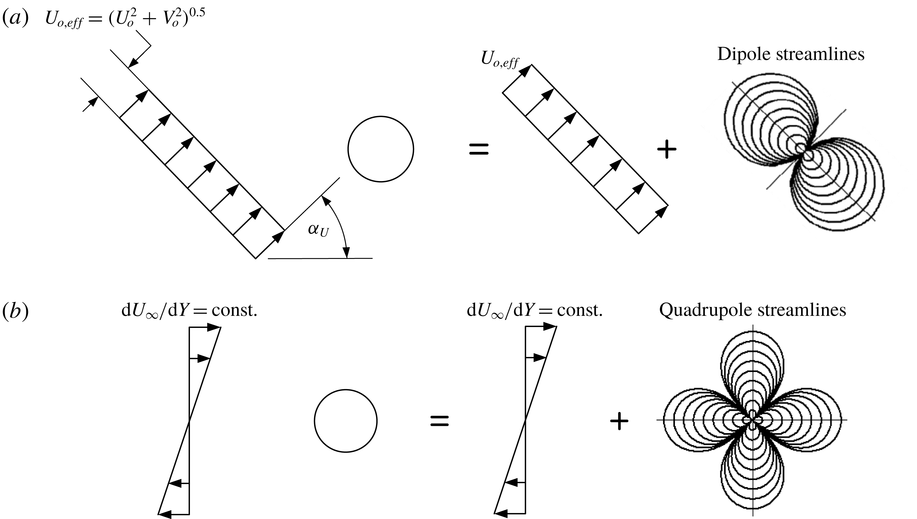
c). This three-component representation may be compacted into two components: one representing uniform flow with effective velocity
 $$\begin{eqnarray}\displaystyle U_{o,eff}=\sqrt{U_{o}^{2}+V_{o}^{2}}, & & \displaystyle\end{eqnarray}$$
over the cylinder at an effective angle of incidence
 $$\begin{eqnarray}\displaystyle & \displaystyle \unicode[STIX]{x1D6FC}_{U}=\tan ^{-1}\left(\frac{V_{o}}{U_{o}}\right), & \displaystyle\end{eqnarray}$$
as depicted in figure 3(a), and the other is centred uniform-shear flow (figure 3
b). It is important to note that as far as the overall approach stream is concerned,
 $\unicode[STIX]{x1D6FC}_{U}$
of the uniform flow subcomponent represents simply a velocity ratio
 $V_{r}=V_{o}/U_{o}$
, rather than an actual incidence angle of the free stream. Specifically, once the shear profile in figure 3(b) is added to the uniform flow in figure 3(a), it is difficult to define a unique approach stream angle since
 $U_{\infty }$
varies in the cross-stream direction, and hence the ratio
 $V_{o}/U_{\infty }$
, which defines the local approach stream angle, also varies across the stream. This variation, however, should become insignificant if the shear rate is sufficiently weak; i.e. in the limit
 $K\rightarrow 0$
. In this limiting flow regime, which we name ‘quasi-uniform’ (QU) flow, the fractional variation in the approach stream velocity over a length comparable with the cylinder diameter is negligible, and an approach stream incidence angle
 $\unicode[STIX]{x1D6FC}$
may be specified with reasonable accuracy; i.e.
 $$\begin{eqnarray}\displaystyle \unicode[STIX]{x1D6FC}\approx \unicode[STIX]{x1D6FC}_{U}. & & \displaystyle\end{eqnarray}$$
Superposition of elemental flows leading to: (a) uniform potential flow with velocity
 $U_{o,eff}$
and angle of incidence
 $\unicode[STIX]{x1D6FC}_{U}$
around a circular cylinder, and (b) centred uniform-shear inviscid flow around a circular cylinder (the cylinder is located on the shear centre, where
 $U_{\infty }=0$
). Superposition of the flows shown in (a) and (b) provides the solution for the cylinder traversing steadily across unbounded uniform-shear flow in the GT frame of reference.

The ability to define an incidence angle for the approach stream is necessary for connecting the moving- and the static-cylinder solutions in the same way the two solutions are connected for uniform free stream. Another significant aspect for making this connection is flow unsteadiness. For the moving cylinder, the velocity
 $U_{o}$
of the uniform approach flow is unsteady because of the movement of the cylinder across the shear. This unsteadiness, which is absent in the case of the non-moving cylinder, could lead to flow dynamics that cause the static- and the moving-cylinder (in the GT frame of reference) solutions to be different, unless the dynamics are sufficiently slow for the flow to be ‘quasi-steady’ (QS). Accordingly, one expects the problem of moving cylinder in shear to asymptotically become similar to that of a static cylinder in the combined limit of quasi-uniformity and quasi-steadiness. This limit is discussed further in § 3.2.
Based on the above, the flow field of the moving cylinder in the GT frame (i.e. in the frame of stationary cylinder) is obtained by superposing two elemental flow fields around a circular cylinder, as depicted in figure 3: a uniform unsteady stream with velocity magnitude
 $U_{o,eff}(t)=\sqrt{U_{o}^{2}(t)+V_{0}^{2}}$
and uniform-flow angle of incidence
 $\unicode[STIX]{x1D6FC}_{U}(t)$
, and a steady centred uniform-shear flow, identical to that of the stationary cylinder. The corresponding velocity field equations in the GT frame (i.e. relative to the cylinder) are found by simply adapting (2.4) and (2.5) to changes in the uniform-stream characteristics,
 $$\begin{eqnarray}\displaystyle & \displaystyle \frac{U_{r}}{U_{o,eff}}=U_{r}^{\ast }=\left(1-\frac{1}{r^{\ast 2}}\right)\cos (\unicode[STIX]{x1D703}-\unicode[STIX]{x1D6FC}_{U})+\frac{K_{eff}}{2}\left(r^{\ast }\sin \unicode[STIX]{x1D703}\cos \unicode[STIX]{x1D703}-\frac{1}{2r^{\ast 3}}\sin 2\unicode[STIX]{x1D703}\right), & \displaystyle\end{eqnarray}$$
 $$\begin{eqnarray}\displaystyle & \displaystyle \frac{U_{\unicode[STIX]{x1D703}}}{U_{o,eff}}=U_{\unicode[STIX]{x1D703}}^{\ast }=-\left(1+\frac{1}{r^{\ast 2}}\right)\sin (\unicode[STIX]{x1D703}-\unicode[STIX]{x1D6FC}_{U})-\frac{K_{eff}}{2}\left(r^{\ast }\sin ^{2}\unicode[STIX]{x1D703}-\frac{1}{2r^{\ast 3}}\cos 2\unicode[STIX]{x1D703}\right). & \displaystyle\end{eqnarray}$$
Equations (2.9) and (2.10) have the same form as (2.4) and (2.5), except for the introduction of
 $\unicode[STIX]{x1D6FC}_{U}$
in the terms representing the potential uniform flow around the cylinder, the change of the normalization velocity scale from
 $U_{o}$
to
 $U_{o,eff}$
, and the change of
 $K$
to
 $K_{eff}$
,
 $$\begin{eqnarray}\displaystyle & \displaystyle K_{eff}=\frac{\text{d}U_{\infty }}{\text{d}Y}\frac{d}{U_{o,eff}}=\frac{md}{U_{o,eff}}. & \displaystyle\end{eqnarray}$$
The moving-cylinder effective non-dimensional shear rate is connected to that of the stationary-cylinder as follows:
 $$\begin{eqnarray}\displaystyle K_{eff}=\frac{\text{d}U_{\infty }}{\text{d}Y}\frac{d}{U_{o,eff}}=\frac{md}{U_{o}}\frac{U_{o}}{U_{o,eff}}=K\cos (\unicode[STIX]{x1D6FC}_{U}). & & \displaystyle\end{eqnarray}$$
Also, introducing
 $$\begin{eqnarray}\displaystyle & \displaystyle K_{eff,max}=\frac{md}{V_{o}}, & \displaystyle\end{eqnarray}$$
the maximum value of
 $K_{eff}$
reached at the shear centre (where the effective reference velocity has its lowest value
 $U_{o,eff}=V_{o}$
), it can be shown that,
 $$\begin{eqnarray}\displaystyle & \displaystyle K_{eff}=\frac{2K_{eff,max}}{\sqrt{\left(Y_{o}^{\ast }K_{eff,max}\right)^{2}+4}}, & \displaystyle\end{eqnarray}$$
 $$\begin{eqnarray}\displaystyle & \displaystyle \tan (\unicode[STIX]{x1D6FC}_{U})=\frac{2}{Y_{o}^{\ast }K_{eff,max}}. & \displaystyle\end{eqnarray}$$
Equations (2.14) and (2.15) show that, for a particular value of
 $K_{eff,max}$
(which is a constant parameter for a given problem),
 $K_{eff}(t)$
and
 $\unicode[STIX]{x1D6FC}_{U}(t)$
, the only parameters required for obtaining the velocity field at any time instant, are ‘set’ by the instantaneous position of the cylinder
 $Y_{o}^{\ast }$
. Equation (2.14) also shows that as the cylinder moves from infinity towards the shear centre,
 $K_{eff}$
changes from zero to
 $K_{eff,max}$
. Concurrently, per (2.15), the angle of the uniform component of the approach stream changes from zero to
 $\unicode[STIX]{x03C0}/2$
(i.e. the velocity ratio
 $V_{r}$
changes from zero to infinity). This variation in
 $\unicode[STIX]{x1D6FC}_{U}$
is consistent with the monotonic decrease in
 $U_{o}$
from an infinite value to zero, with
 $V_{o}$
remaining constant.
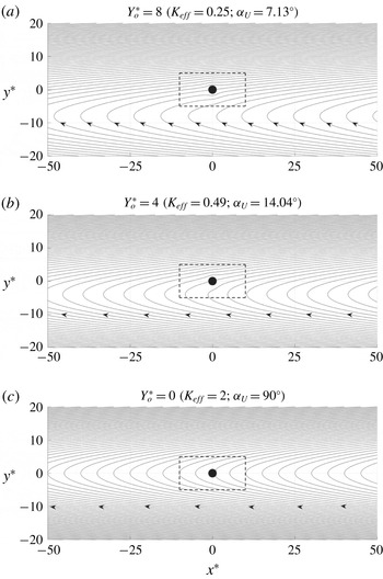
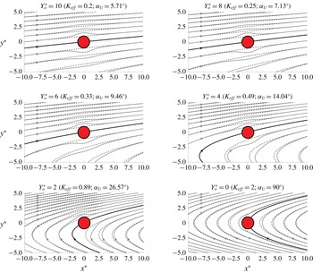
Figures 4 and 5 display snapshots of the streamlines of the flow around the cylinder in the GT reference frame, based on (2.9) and (2.10), as the cylinder traverses across the approach shear flow from
 $Y_{o}^{\ast }=10$
to 0, for
 $K_{eff,max}=2$
. The plots in figure 4 provide a global view of the flow to depict the character of the approach undisturbed stream at three time instants where the cylinder is located at
 $Y_{o}^{\ast }=8,4$
and 0. A close-up view of the streamlines in proximity of the cylinder (within the window delineated by the broken line in figure 4) is given in figure 5 at the same locations, as well as at
 $Y_{o}^{\ast }=10$
, 6 and 2. For these plots, the thick black line highlights the stagnation streamline, and the solid grey and broken black lines depict the streamlines with and without the cylinder presence, respectively.
Figure 4 shows that, in the GT frame of reference, the approach stream originates from the bottom half of the domain
 $(x^{\ast }\rightarrow \infty ,y^{\ast }<0)$
regardless of the position of the cylinder. The undisturbed-flow streamlines are parabolic (which can be shown by considering the stream function in the limit
 $r^{\ast }\rightarrow \infty$
), making the approach stream conditions fundamentally different from those for a stationary cylinder at the same instantaneous
 $Y_{o}^{\ast }$
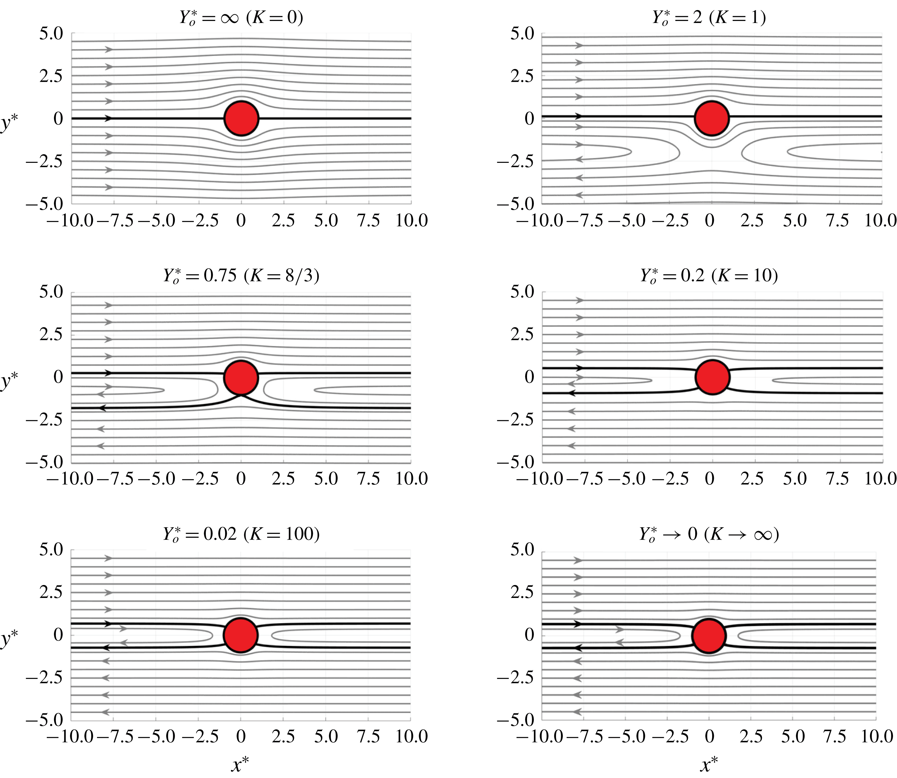
of the moving cylinder (see the streamlines far away from the non-moving cylinder in figure 6). This shows that, generally speaking, the problem of a moving cylinder in uniform-shear free stream cannot simply be addressed via a rotation of the approach stream of the static cylinder. However, inspection of figure 5 shows that when the cylinder is sufficiently far from the shear centre (
 $Y_{o}^{\ast }=8$
and 10), undisturbed approach stream conditions with approximately parallel and straight streamlines can be found to the left of the cylinder. Hence, one may define the approach flow at a short distance upstream of the cylinder in the
 $y^{\ast }>0$
half-plane; rather than based on tracking the approach stream to its origin in the
 $y^{\ast }<0$
half-plane. Under these conditions (large
 $Y_{o}^{\ast }$
; and small
 $K_{eff}$
and
 $\unicode[STIX]{x1D6FC}_{U}$
), the static-cylinder results may be usable in solving the moving-cylinder problem (this point is addressed more generally in §§ 3.1 and 3.2). As
 $Y_{o}^{\ast }$
decreases (and
 $K_{eff}$
and
 $\unicode[STIX]{x1D6FC}_{U}$
increase), the approach streamlines become more curved and the fore (left) stagnation point progressively moves along the bottom surface away from the cylinder’s leading edge, eventually switching to the rear side of the surface, as exemplified at the terminal location
 $Y_{o}^{\ast }=0$
.
Streamlines of the flow around a cylinder traversing across positive uniform-shear approach flow in the GT frame of reference (
 $K_{eff,max}=2$
). Plots correspond to cylinder locations of (a)
 $Y_{o}^{\ast }=8$
, (b) 4 and (c) 0. The corresponding effective non-dimensional shear rate and uniform-flow angle of incidence, as given by (2.14) and (2.15), respectively, are indicated in parenthesis.

Streamlines in the GT reference frame of the flow around a cylinder traversing across positive uniform-shear approach flow from
 $Y_{o}^{\ast }=10$
to 0 in steps of
 $-2$
(
 $K_{eff,max}=2$
). Different subplots depict the flow at different instants of the cylinder motion, as given by the cylinder cross-stream position on top of the plot. The corresponding effective non-dimensional shear rate and uniform-flow angle of incidence, as given by (2.14) and (2.15), respectively, are indicated in parenthesis. Broken lines show the streamlines if the cylinder were absent, and the thick line depicts the stagnation streamline.

Streamlines of the flow around a stationary cylinder in a positive uniform-shear approach flow. Different subplots depict the flow for different values of the non-dimensional shear rate
 $K$
. The corresponding non-dimensional cross-stream location of the cylinder, as given by (1.2), is also indicated. The thick line depicts the stagnation streamline.

2.2 Surface pressure and force
For 2-D unsteady incompressible inviscid flow, the pressure and the velocity fields are connected through the unsteady Bernoulli equation. Following Milne-Thomson (Reference Milne-Thomson1996, p. 115, equation (2)), the equation may be written as follows:
 $$\begin{eqnarray}\displaystyle & \displaystyle \frac{p}{\unicode[STIX]{x1D70C}}+\frac{1}{2}Q^{2}+gz-\int _{AP}\unicode[STIX]{x1D6FB}^{2}\unicode[STIX]{x1D713}\,\text{d}\unicode[STIX]{x1D713}+\int _{AP}\frac{\unicode[STIX]{x2202}Q_{s}}{\unicode[STIX]{x2202}t}\,\text{d}s=f(t), & \displaystyle\end{eqnarray}$$
where,
 $AP$
is a fixed arbitrary path within the flow field,
 $p$
is pressure,
 $Q$
is velocity vector magnitude,
 $gz$
is gravity force potential per unit mass, s is coordinate measured along
 $AP$
,
 $Q_{s}$
is the velocity component tangent to
 $AP$
and f is an arbitrary function of time. Equation (2.16) may be written as a definite integral between points 1 and 2 on curve
 $AP$
as follows (ignoring gravity),
 $$\begin{eqnarray}\displaystyle & \displaystyle \frac{p_{2}}{\unicode[STIX]{x1D70C}}-\frac{p_{1}}{\unicode[STIX]{x1D70C}}+\frac{1}{2}(Q_{2}^{2}-Q_{1}^{2})-\int _{1}^{2}\unicode[STIX]{x1D6FB}^{2}\unicode[STIX]{x1D713}\,\text{d}\unicode[STIX]{x1D713}+\int _{1}^{2}\frac{\unicode[STIX]{x2202}Q_{s}}{\unicode[STIX]{x2202}t}\,\text{d}s=0. & \displaystyle\end{eqnarray}$$
Normalizing (2.17) using
 $d/2$
and
 $U_{o,eff}$
as length and velocity scales, respectively, leads to (see appendix A),
 $$\begin{eqnarray}\displaystyle \displaystyle C_{p} & = & \displaystyle \frac{p_{2}-p_{1}}{\frac{1}{2}\unicode[STIX]{x1D70C}U_{o,eff}^{2}}=(Q_{1}^{\ast 2}-Q_{2}^{\ast 2})+2\int _{1}^{2}\unicode[STIX]{x1D6FB}^{\ast 2}\unicode[STIX]{x1D713}^{\ast }\,\text{d}\unicode[STIX]{x1D713}^{\ast }-\frac{d}{U_{o,eff}}\int _{1}^{2}\frac{\unicode[STIX]{x2202}Q_{s}^{\ast }}{\unicode[STIX]{x2202}t}\,\text{d}s^{\ast }\nonumber\\ \displaystyle & & \displaystyle +\,K_{eff}\cos (\unicode[STIX]{x1D6FC}_{U})\sin (\unicode[STIX]{x1D6FC}_{U})\int _{1}^{2}Q_{s}^{\ast }\,\text{d}s^{\ast },\end{eqnarray}$$
where,
 $C_{p}$
is a pressure coefficient. For steady flow, points 1 and 2 in (2.17) are usually taken on a streamline (i.e.
 $d\unicode[STIX]{x1D713}=0$
), which eliminates the integral terms in the equation, simplifying its use. However, this approach is more complicated for the moving cylinder in uniform-shear flow since the streamlines are unsteady, as seen in figure 5. Therefore, to simplify the calculation, a fixed integration path, depicted in figure 1(b), is utilized. This path consists of two different segments: (i) a straight line coincident with the negative x axis connecting the pressure at a far upstream point
 $\infty$
to that at the cylinder’s leading edge
 $le$
, and (ii) a circular-arc path coincident with the cylinder’s surface, connecting
 $le$
to an arbitrary point c on the cylinder’s surface. This process leads to the overall surface pressure coefficient, given by,
 $$\begin{eqnarray}\displaystyle C_{pc}(\unicode[STIX]{x1D703})=C_{ple}+C_{pc,le}(\unicode[STIX]{x1D703}), & & \displaystyle\end{eqnarray}$$
where, the first and second terms on the right-hand side of (2.19) are obtained by applying (2.18) between points
 $\infty$
and
 $le$
, and
 $le$
and c, respectively. Dropping the subscript c, with the understanding that
 $C_{p}$
is only computed on the cylinder surface in the present work, evaluating (2.18) for each of the two terms on the right-hand side of (2.19), and adding the results leads to,
 $$\begin{eqnarray}\displaystyle \displaystyle C_{p}(\unicode[STIX]{x1D703},t) & = & \displaystyle \frac{p(\unicode[STIX]{x1D703},t)-p_{\infty }}{\frac{1}{2}\unicode[STIX]{x1D70C}U_{o,eff}^{2}(t)}=[1-4\,\sin ^{2}(\unicode[STIX]{x1D703}-\unicode[STIX]{x1D6FC}_{U}(t))]+2K_{eff}(t)\nonumber\\ \displaystyle & & \displaystyle \left[\sin (\unicode[STIX]{x1D6FC}_{U}(t))\cos (\unicode[STIX]{x1D703})-\sin (\unicode[STIX]{x1D703}-\unicode[STIX]{x1D6FC}_{U}(t))\left({\textstyle \frac{1}{2}}-\cos (2\unicode[STIX]{x1D703})\right)\right]\nonumber\\ \displaystyle & & \displaystyle +\,\displaystyle \frac{K_{eff}^{2}(t)}{16}[1+4\cos (2\unicode[STIX]{x1D703})-4\cos ^{2}(2\unicode[STIX]{x1D703})].\end{eqnarray}$$
The form of equation (2.20) is checked in two different ways. First, by verifying that the form simplifies to the correct form of the simpler cases of a static cylinder in shear flow and in uniform flow (these details are provided in appendix B). Second, by comparing the force acting on the moving cylinder in shear when computed using (2.20), see below, with that obtained using a different approach (see § 3.2).
Given the parabolic streamlines of the approach flow, as revealed in figure 4, it is not possible to define a unique direction of the approach stream relative to the moving cylinder; i.e. in the GT frame of reference. In turn, this makes it infeasible to define the directions of the lift and the drag components of the force acting on the moving cylinder based on free stream direction. However, for the purpose of the present discussion, we will define the lift and the drag in a time-invariant coordinate system in the directions perpendicular and parallel, respectively, to the approach stream in the laboratory frame of reference. With this in mind, the
 $x$
(drag) and
 $y$
(lift) force coefficients are computed from integration of the pressure coefficient around the cylinder as follows:
 $$\begin{eqnarray}\displaystyle & \displaystyle C_{D}=C_{x}=\frac{F_{x}}{\frac{1}{2}\unicode[STIX]{x1D70C}U_{o,eff}^{2}d}=-\frac{1}{2}\int _{0}^{2\unicode[STIX]{x03C0}}\frac{p-p_{\infty }}{\frac{1}{2}\unicode[STIX]{x1D70C}U_{o,eff}^{2}}\cos (\unicode[STIX]{x1D703})\,\text{d}\unicode[STIX]{x1D703}=-\frac{1}{2}\int _{0}^{2\unicode[STIX]{x03C0}}C_{p}\cos (\unicode[STIX]{x1D703})\,\text{d}\unicode[STIX]{x1D703},\quad & \displaystyle\end{eqnarray}$$
 $$\begin{eqnarray}\displaystyle & \displaystyle C_{L}=C_{y}=\frac{F_{y}}{\frac{1}{2}\unicode[STIX]{x1D70C}U_{o,eff}^{2}d}=-\frac{1}{2}\int _{0}^{2\unicode[STIX]{x03C0}}\frac{p-p_{\infty }}{\frac{1}{2}\unicode[STIX]{x1D70C}U_{o,eff}^{2}}\sin (\unicode[STIX]{x1D703})\,\text{d}\unicode[STIX]{x1D703}=-\frac{1}{2}\int _{0}^{2\unicode[STIX]{x03C0}}C_{p}\sin (\unicode[STIX]{x1D703})\,\text{d}\unicode[STIX]{x1D703}.\quad & \displaystyle\end{eqnarray}$$
Substitution of (2.20) in (2.21) and (2.22), yields,
 $$\begin{eqnarray}\displaystyle & \displaystyle C_{D}=C_{x}=-\unicode[STIX]{x03C0}K_{eff}\sin (\unicode[STIX]{x1D6FC}_{U}), & \displaystyle\end{eqnarray}$$
 $$\begin{eqnarray}\displaystyle & \displaystyle C_{L}=C_{y}=\unicode[STIX]{x03C0}K_{eff}\cos (\unicode[STIX]{x1D6FC}_{U}). & \displaystyle\end{eqnarray}$$
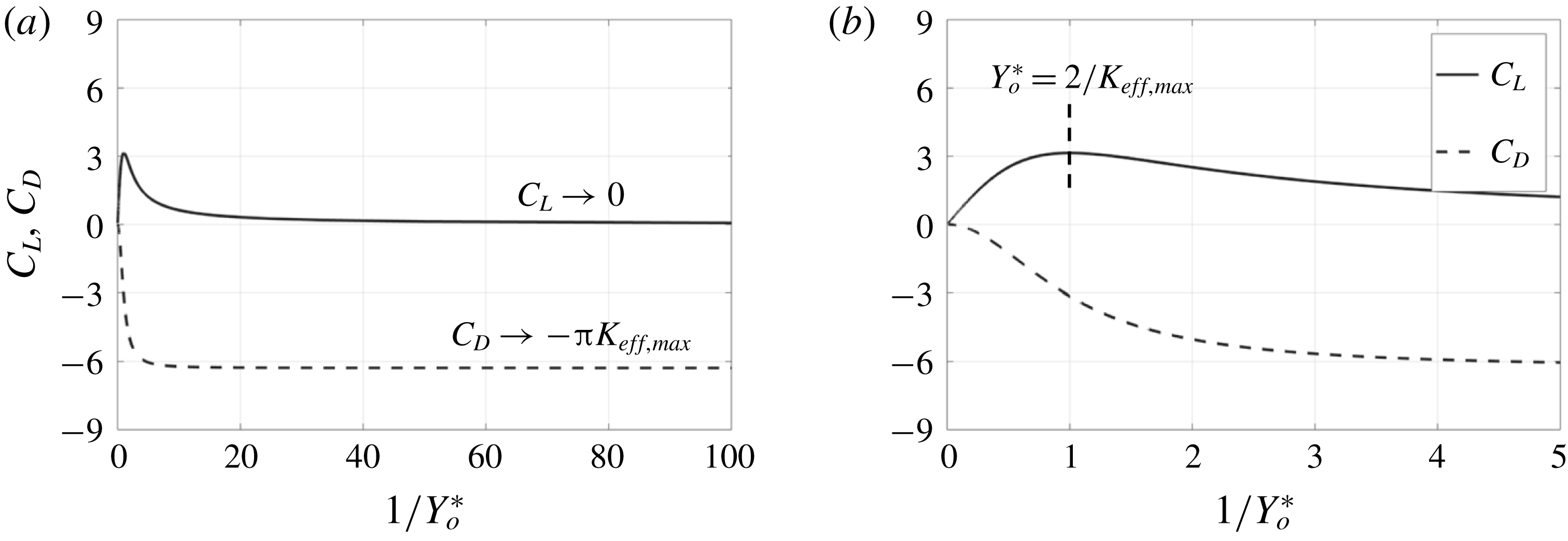
Equations (2.23) and (2.24) are evaluated for the moving cylinder case considered in figures 4 and 5 (
 $K_{eff,max}=2$
). The results are displayed in figure 7 versus the cross-stream position of the cylinder, plotted as
 $Y_{o}^{\ast -1}$
so that the increase of the abscissa variable also indicates time increase. The figure contains two plots, one showing the evolution of the force coefficients as the cylinder traverses across the shear from infinity to zero. This plot is truncated at
 $Y_{o}^{\ast -1}=100$
(
 $Y_{o}^{\ast }=0.01$
), since the force coefficients have practically reached an asymptotic state by then. The other plot provides a magnified view of the time period over which most of the force variation takes place.
History of the
 $x$
and
 $y$
force coefficients for a moving cylinder in uniform-shear flow (
 $K_{eff,max}=2$
). During the motion, the cylinder cross-stream location
 $Y_{o}^{\ast }$
decreases from
 $\infty$
to 0, while the abscissa
 $Y_{o}^{\ast -1}$
increases monotonically with time. (a) Motion history truncated at
 $Y_{o}^{\ast }=0.01$
, (b) a magnified view of the history in (a).

As seen from figure 7, initially
 $C_{L}$
increases with time, reaching a maximum value at
 $Y_{o}^{\ast }=2/K_{eff,max}$
, which in this figure occurs one radius away (
 $Y_{o}^{\ast }=1$
) from the shear centre, before decaying towards zero as the cylinder approaches
 $Y_{o}^{\ast }=0$
. The presence of maximum lift coefficient is due to the competing effects of
 $K_{eff}$
and
 $\unicode[STIX]{x1D6FC}_{U}$
. Specifically, as time progresses,
 $Y_{o}^{\ast }$
decreases, causing
 $\unicode[STIX]{x1D6FC}_{U}$
to increase (from
 $0^{\circ }$
to
 $90^{\circ }$
; per equation (2.15)) with corresponding decrease in
 $\cos (\unicode[STIX]{x1D6FC}_{U})$
and
 $C_{L}$
(2.24). This decrease is opposed by the monotonic increase in
 $K_{eff}$
from 0 to
 $K_{eff,max}$
(2.14), which increases
 $C_{L}$
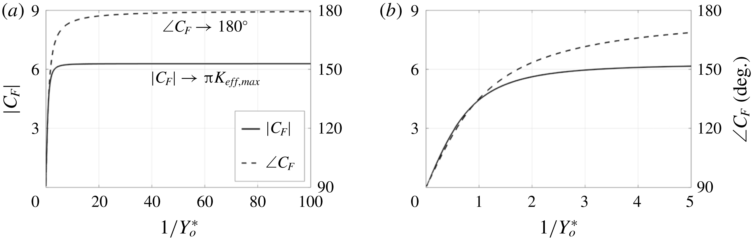
. The nature of these variations may be understood more clearly by considering the magnitude and angle of the overall force vector coefficient; given by, respectively,
 $$\begin{eqnarray}\displaystyle & \displaystyle |C_{F}|=\sqrt{C_{D}^{2}+C_{L}^{2}}=\unicode[STIX]{x03C0}K_{eff}, & \displaystyle\end{eqnarray}$$
 $$\begin{eqnarray}\displaystyle & \displaystyle \angle C_{F}=\tan ^{-1}\left(\frac{C_{L}}{C_{D}}\right)=\frac{\unicode[STIX]{x03C0}}{2}+\unicode[STIX]{x1D6FC}_{U}. & \displaystyle\end{eqnarray}$$
Equations (2.25) and (2.26) are evaluated and plotted in figure 8. As seen from the figure, and the equations, the magnitude of the force increases monotonically with time due to the monotonic increase of
 $|C_{F}|$
with
 $K_{eff}$
. However, since the force angle is initially aligned with the lift direction (
 $\angle C_{F}=\unicode[STIX]{x03C0}/2$
), all of the force is directed towards lift. As time progresses, the force vector rotates to eventually point in the negative x direction at the end of the motion. Thus, though the force magnitude increases with time, the fraction of the force producing lift becomes smaller and smaller with increasing time. Initially, the force increase due to the rise in the non-dimensional shear rate dominates, resulting in the initial rise in
 $C_{L}$
. Eventually, the turning of the force vector becomes more important, resulting in the observed maximum
 $C_{L}$
in figure 7. The turnaround point can be shown to happen at
 $Y_{o}^{\ast }=2/K_{eff,max}$
, which equals unity in the particular example considered here, where
 $K_{eff,max}=2$
.
History of the force coefficient magnitude (
 $|C_{F}|$
) and angle (
 $\angle C_{F}$
) for a moving cylinder in uniform-shear flow (
 $K_{eff,max}=2$
). During the motion, the cylinder cross-stream location
 $Y_{o}^{\ast }$
decreases from
 $\infty$
to 0. The abscissa
 $Y_{o}^{\ast -1}$
increases monotonically with time. (a) Motion history truncated at
 $Y_{o}^{\ast }=0.01$
, (b) a magnified view of the history in (a).

Unlike
 $C_{L}$
, the magnitude of
 $C_{D}$
increases monotonically from zero at the start of the motion
 $(Y_{o}^{\ast }=\infty )$
, to a finite value at the end of the motion (figure 7). Remarkably, the drag coefficient has a negative sign throughout the motion, indicating the development of thrust. Initially, this thrust is zero since
 $K_{eff}\rightarrow 0$
as
 $Y_{o}^{\ast }\rightarrow \infty$
, corresponding to uniform flow. However, as time progresses and
 $K_{eff}$
increases, the thrust becomes increasingly significant, reaching its maximum value at the end of the motion, where
 $K_{eff}$
has its peak value, and hence
 $|C_{F}|$
is largest (2.25), and all of the force is directed towards thrust (2.26). The physics underlying the observed force behaviour is discussed in the following section.
3 Discussion
3.1 Physics of force generation
Though it may not be immediately evident, the force results, (2.25) and (2.26), are rather surprising. Specifically, the magnitude and the direction of the force are exactly the same as those acting on a static cylinder placed in uniform-shear approach flow with angle of incidence
 $\unicode[STIX]{x1D6FC}=\unicode[STIX]{x1D6FC}_{U}$
and non-dimensional shear rate
 $K=K_{eff}$
. More specifically, the results of Tsien (Reference Tsien1943) show that such a cylinder exhibits no drag (
 $C_{D}=0$
), while experiencing a lift coefficient
 $C_{L}=\unicode[STIX]{x03C0}K$
. Taking into account the approach stream’s angle of incidence and the non-dimensional shear rate based on the total reference velocity magnitude (
 $U_{o,eff}$
), the static cylinder’s lift coefficient is identical to
 $C_{F}$
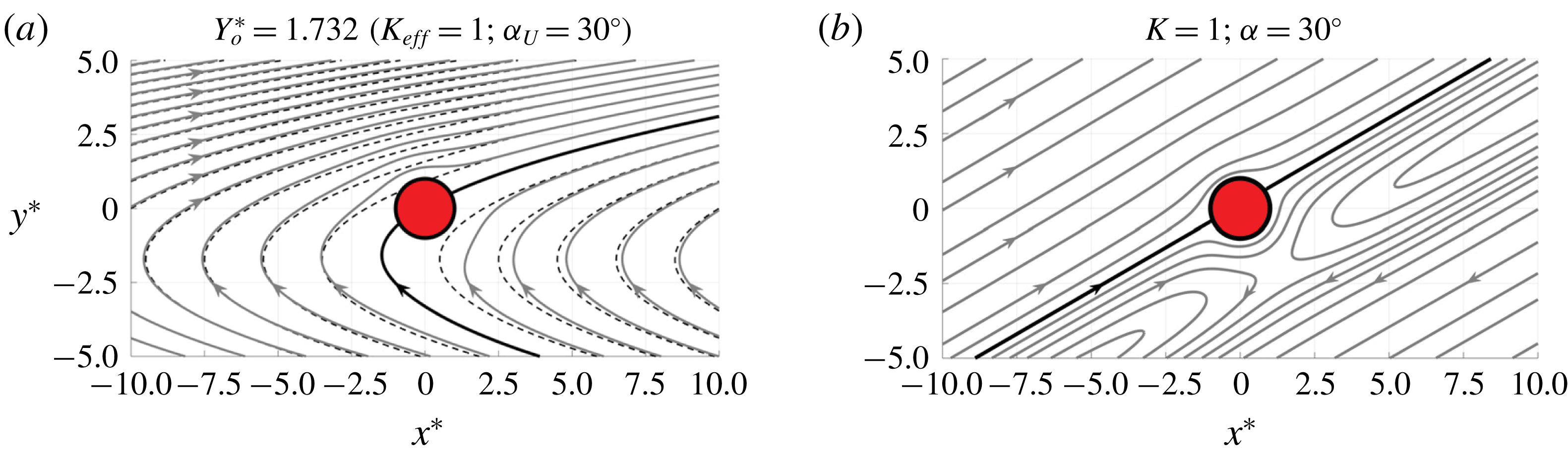
in (2.25) and (2.26). This outcome is not expected since the comparison of the streamlines for the moving cylinder, in a Galilean-transformed frame of reference (figures 4 and 5), to the stationary-cylinder’s streamlines (figure 6) demonstrates two flow fields that cannot be made the same by changing the angle of incidence and the velocity magnitude of the static-cylinder’s approach stream. To give a more specific example, the streamlines for the moving cylinder when
 $K_{eff}=1$
and
 $\unicode[STIX]{x1D6FC}_{U}=30^{\circ }$
are shown in figure 9(a), compared to those obtained from rotating the static-cylinder’s flow field for
 $K=1$
by an angle of incidence of
 $30^{\circ }$
in figure 9(b). While the force acting on the cylinder is the same for both cases, the flow fields are significantly different.
Comparison between the streamlines around the moving cylinder (a) when located at
 $Y_{o}^{\ast }=1.732$
(
 $K_{eff,max}=2$
) with those around a static cylinder, (b) having the same approach stream’s non-dimensional shear rate and angle of incidence as the instantaneous
 $K_{eff}$
and
 $\unicode[STIX]{x1D6FC}_{U}$
values for the moving cylinder. Broken lines show the streamlines if the cylinder were absent, and the dark line depicts the stagnation streamline.

The surface-pressure coefficient distributions corresponding to the two flow fields in figure 9 are compared in figure 10. For the moving cylinder, the distribution is obtained using (2.20), while for the static cylinder (B1) is used after replacing
 $\unicode[STIX]{x1D703}$
with
 $\unicode[STIX]{x1D703}-\unicode[STIX]{x1D6FC}_{U}$
to account for the incidence angle of the flow. In figure 10, two different plots of the
 $C_{p}$
distributions are given: (a) one versus
 $x^{\ast }$
and (b) the other versus
 $y^{\ast }$
. As explained in the caption, the area encircled by the
 $C_{p}$
distribution equals
 $C_{y}$
and
 $C_{x}$
, for the left and right figures, respectively. Visual inspection of the encircled areas for the moving- and static-cylinder cases confirms that
 $C_{y}>0$
and
 $C_{x}<0$
; in agreement with the results in figure 7 (where for the moving cylinder
 $C_{x}=C_{D}$
and
 $C_{y}=C_{L}$
).
Comparison of the surface
 $C_{p}$
distributions of the moving- and static-cylinder cases considered in figure 9. The distribution is plotted versus (a)
 $x^{\ast }$
and (b)
 $y^{\ast }$
. Solid and broken lines, respectively, depict the
 $C_{p}$
distribution on (a) the upper and lower surface and (b) downstream and upstream surface. The area encircled by the distributions, which is filled for the moving cylinder case, equal to (a)
 $C_{y}$
and (b)
 $C_{x}$
, with the contribution to the force coefficient from an encircled area is positive if the area is bounded by a broken line on top and a solid one on bottom. The circle symbols indicate the location of the front stagnation point.

Figure 10 shows that indeed, consistent with the different flow patterns in figure 9, the surface pressure distribution is different for the moving and the static cylinder. This difference manifests itself not only in different values of
 $C_{p}$
at the same location on the cylinder’s surface but also in the location of the front stagnation point. Figure 10 also gives a visual clue for the reason why the different
 $C_{p}$
distributions yield the same
 $C_{x}$
and
 $C_{y}$
. In particular, notwithstanding the shape difference of the two distributions, the net area encircled by the different distributions does not change. This finding suggests that the mechanisms for force generation may not be the same for the two cases. To gain a deeper insight into these mechanisms in the case of the moving cylinder, the force calculation is revisited using an alternative approach.
For simplification,
 $C_{p}$
is redefined using a reference pressure at the cylinder’s leading edge
 $le$
rather than the upstream undisturbed-flow pressure
 $p_{\infty }$
. The reference pressure value does not influence the computed force at a given time instant, but the magnitude of
 $C_{p}$
is different than that defined in (2.20), which is used throughout the document for plotting the
 $C_{p}$
distribution. With this understanding,
 $C_{p}$
is used to denote the pressure coefficient regardless of the reference pressure value. Applying (2.18) on the surface of the cylinder with point 1 corresponding to
 $le$
(see figure 1
b), point 2 is at a general azimuthal location
 $\unicode[STIX]{x1D703}$
, and denoting the terms associated with the temporal derivative of the velocity (the last two integral terms on the right-hand side of (2.18))
 $C_{p}^{^{\prime }}$
,
 $$\begin{eqnarray}\displaystyle & \displaystyle C_{p}=\frac{p(\unicode[STIX]{x1D703})-p_{le}}{\frac{1}{2}\unicode[STIX]{x1D70C}U_{o,eff}^{2}}=[Q_{le}^{\ast 2}-Q^{\ast 2}(\unicode[STIX]{x1D703})]+C_{p}^{^{\prime }}, & \displaystyle\end{eqnarray}$$
where the integral term involving the stream function vanishes since the cylinder surface is a streamline. Recognizing that only the azimuthal component of velocity
 $U_{\unicode[STIX]{x1D703}}$
is non-zero on the cylinder’s surface, (3.1) becomes,
 $$\begin{eqnarray}\displaystyle & \displaystyle C_{p}=\frac{p(\unicode[STIX]{x1D703})-p_{le}}{\frac{1}{2}\unicode[STIX]{x1D70C}U_{o,eff}^{2}}=[U_{\unicode[STIX]{x1D703}le}^{\ast 2}-U_{\unicode[STIX]{x1D703}}^{\ast 2}(\unicode[STIX]{x1D703})]+C_{p}^{^{\prime }}. & \displaystyle\end{eqnarray}$$
To proceed further, and differently from before, the flow is decomposed into two flow problems around a stationary cylinder (in a Galilean frame): one that arises from a streamwise (x) approach stream consisting of uniform flow
 $U_{o}$
superposed on uniform-shear (Tsien’s problem), and the other associated with a cross-stream (y) uniform approach stream
 $V_{o}$
. Though this way of decomposition (see figure 11) is different from that followed so far (figure 3), the two decompositions clearly correspond to the same overall velocity field. The new superposition leads to,
 $$\begin{eqnarray}\displaystyle U_{\unicode[STIX]{x1D703}}^{\ast }=U_{T\unicode[STIX]{x1D703}}^{\ast }+U_{V\unicode[STIX]{x1D703}}^{\ast }, & & \displaystyle\end{eqnarray}$$
where subscripts
 $T$
and
 $V$
denote Tsien’s and the cross-stream uniform flow, respectively. Substituting (3.3) in (3.2) and rearranging terms gives
 $$\begin{eqnarray}\displaystyle C_{p}=[U_{T\unicode[STIX]{x1D703}le}^{\ast 2}-U_{T\unicode[STIX]{x1D703}}^{\ast 2}(\unicode[STIX]{x1D703})]+[U_{V\unicode[STIX]{x1D703}le}^{\ast 2}-U_{V\unicode[STIX]{x1D703}}^{\ast 2}(\unicode[STIX]{x1D703})]+2\ast [U_{T\unicode[STIX]{x1D703}le}^{\ast }U_{V\unicode[STIX]{x1D703}le}^{\ast }-U_{T\unicode[STIX]{x1D703}}^{\ast }U_{V\unicode[STIX]{x1D703}}^{\ast }]+C_{p}^{^{\prime }}. & & \displaystyle\end{eqnarray}$$
Superposition of elemental flows leading to: (a) uniform potential flow with
 $90^{\circ }$
angle of incidence around a circular cylinder, and (b) uniform-shear inviscid flow around a circular cylinder (the cylinder is located off the shear centre: Tsien’s (Reference Tsien1943) problem).

As given by (3.2),
 $U_{o,eff}$
is the velocity scale used for normalizing the pressure. To connect the different terms in (3.4) to the
 $C_{p}$
distribution of the ‘component problems’, the velocity scale should be changed to
 $U_{o}$
for Tsien’s flow, and
 $V_{o}$
for the cross-stream uniform flow. This changes (3.4) to the following:
 $$\begin{eqnarray}\displaystyle C_{p} & = & \displaystyle \displaystyle \frac{U_{o}^{2}}{U_{o,eff}^{2}}\left[\left(\frac{U_{T\unicode[STIX]{x1D703}le}}{U_{o}}\right)^{2}-\left(\frac{U_{T\unicode[STIX]{x1D703}}}{U_{o}}\right)^{2}\right]+\frac{V_{o}^{2}}{U_{o_{eff}}^{2}}\left[\left(\frac{U_{V\unicode[STIX]{x1D703}le}}{V_{o}}\right)^{2}-\left(\frac{U_{V\unicode[STIX]{x1D703}}}{V_{o}}\right)^{2}\right]\nonumber\\ \displaystyle & & \displaystyle +\,2\ast \frac{U_{o}}{U_{o,eff}}\frac{V_{o}}{U_{o,eff}}\left[\frac{U_{T\unicode[STIX]{x1D703}le}}{U_{o}}\frac{U_{V\unicode[STIX]{x1D703}le}}{V_{o}}-\frac{U_{T\unicode[STIX]{x1D703}}}{U_{o}}\frac{U_{V\unicode[STIX]{x1D703}}}{V_{o}}\right]+C_{p}^{^{\prime }}.\end{eqnarray}$$
Recognizing that
 $U_{o}/U_{o,eff}=\cos (\unicode[STIX]{x1D6FC}_{U})$
and
 $V_{o}/U_{o,eff}=\sin (\unicode[STIX]{x1D6FC}_{U})$
,
 $$\begin{eqnarray}\displaystyle C_{p}=\cos ^{2}(\unicode[STIX]{x1D6FC}_{U})C_{pT}+\sin ^{2}(\unicode[STIX]{x1D6FC}_{U})C_{pV}+2\cos (\unicode[STIX]{x1D6FC}_{U})\sin (\unicode[STIX]{x1D6FC}_{U})C_{pTV}+C_{p}^{^{\prime }}, & & \displaystyle\end{eqnarray}$$
where,
 $C_{pT}$
,
 $C_{pV}$
and
 $C_{pTV}$
correspond to the respective quantities in square brackets in (3.5). Physically,
 $C_{pT}$
and
 $C_{pV}$
are, respectively, the pressure coefficients for Tsien’s flow and uniform flow over a cylinder at
 $90^{\circ }$
incidence, both of which are known. On the other hand,
 $C_{pTV}$
is an unknown pressure coefficient that involves terms from both flow fields. Also recall that
 $C_{p}^{^{\prime }}$
represents terms due to the temporal derivative of the flow field.
To obtain the force coefficients, (3.6) may be substituted in integrals (2.21) and (2.22), respectively. Since it is well known that steady, inviscid uniform flow around a circular cylinder does not result in any forces, the term involving
 $C_{pV}$
in (3.6) does not contribute to
 $C_{x}$
and
 $C_{y}$
. Similarly, substituting
 $C_{pTV}$
in (2.21) and (2.22) results in zero force coefficients. Thus, one may express
 $C_{x}$
and
 $C_{y}$
as follows:
 $$\begin{eqnarray}\displaystyle & \displaystyle C_{x}=-\frac{1}{2}\left[\cos ^{2}(\unicode[STIX]{x1D6FC}_{U})\int _{0}^{2\unicode[STIX]{x03C0}}C_{pT}\cos (\unicode[STIX]{x1D703})\,\text{d}\unicode[STIX]{x1D703}+\int _{0}^{2\unicode[STIX]{x03C0}}{C^{^{\prime }}}_{p}\cos (\unicode[STIX]{x1D703})\,\text{d}\unicode[STIX]{x1D703}\right]=\cos ^{2}(\unicode[STIX]{x1D6FC}_{U})C_{xT}+C_{x}^{^{\prime }},\quad & \displaystyle\end{eqnarray}$$
 $$\begin{eqnarray}\displaystyle & \displaystyle C_{y}=-\frac{1}{2}\left[\cos ^{2}(\unicode[STIX]{x1D6FC}_{U})\int _{0}^{2\unicode[STIX]{x03C0}}C_{pT}\sin (\unicode[STIX]{x1D703})\,\text{d}\unicode[STIX]{x1D703}+\int _{0}^{2\unicode[STIX]{x03C0}}{C^{^{\prime }}}_{p}\sin (\unicode[STIX]{x1D703})\,\text{d}\unicode[STIX]{x1D703}\right]=\cos ^{2}(\unicode[STIX]{x1D6FC}_{U})C_{yT}+C_{y}^{^{\prime }}.\qquad & \displaystyle\end{eqnarray}$$
That is, the force coefficients are due to the superposition of those arising from Tsien’s flow and the temporal derivative of the velocity. Following Tsien (Reference Tsien1943) we have,
 $$\begin{eqnarray}\displaystyle & \displaystyle C_{xT}=0, & \displaystyle\end{eqnarray}$$
 $$\begin{eqnarray}\displaystyle & \displaystyle C_{yT}=\unicode[STIX]{x03C0}K. & \displaystyle\end{eqnarray}$$
On the other hand, to find the force coefficients
 $C_{x}^{^{\prime }}$
and
 $C_{y}^{^{\prime }}$
, it is recognized that the only approach flow component contributing to the unsteady force is that due to the uniform flow
 $U_{o}(t)$
. This is a classical problem in unsteady fluid dynamics, where the flow unsteadiness results in the development of drag (
 $C_{x}$
) but no lift. The drag force is known to arise from, and to act in the direction of, fluid acceleration. The specific form of the forces in this case is given by (e.g. see equation (2)–(33) in Blevins (Reference Blevins2001)),
 $$\begin{eqnarray}\displaystyle & \displaystyle F_{x}=2\unicode[STIX]{x1D70C}\unicode[STIX]{x03C0}\left(\frac{d}{2}\right)^{2}\frac{\text{d}U_{o}}{\text{d}t}, & \displaystyle\end{eqnarray}$$
 $$\begin{eqnarray}\displaystyle & \displaystyle F_{y}=0, & \displaystyle\end{eqnarray}$$
which lead to,
 $$\begin{eqnarray}\displaystyle & \displaystyle C_{x}^{\prime }=\frac{F_{x}}{\frac{1}{2}\unicode[STIX]{x1D70C}U_{o,eff}^{2}d}=\frac{\unicode[STIX]{x03C0}d(-mV_{o})}{U_{o,eff}^{2}}=-\unicode[STIX]{x03C0}\left(\frac{md}{U_{o,eff}}\right)\left(\frac{V_{o}}{U_{o,eff}}\right)=-\unicode[STIX]{x03C0}K_{eff}\sin (\unicode[STIX]{x1D6FC}_{U}), & \displaystyle\end{eqnarray}$$
 $$\begin{eqnarray}\displaystyle & \displaystyle C_{y}^{\prime }=0. & \displaystyle\end{eqnarray}$$
Substituting (3.9), (3.10), (3.13) and (3.14) into (3.7) and (3.8),
 $$\begin{eqnarray}\displaystyle & \displaystyle C_{x}=-\unicode[STIX]{x03C0}K_{eff}\sin (\unicode[STIX]{x1D6FC}_{U}), & \displaystyle\end{eqnarray}$$
 $$\begin{eqnarray}\displaystyle & \displaystyle C_{y}=\unicode[STIX]{x03C0}K\cos ^{2}(\unicode[STIX]{x1D6FC}_{U})=\unicode[STIX]{x03C0}K_{eff}\cos (\unicode[STIX]{x1D6FC}_{U}). & \displaystyle\end{eqnarray}$$
Equations (3.15) and (3.16) are precisely the same as (2.23) and (2.24), which are derived from a relatively lengthy process in which the cylinder’s pressure distribution is first obtained and then integrated around the cylinder to arrive at the net force. As such, the present succinct approach provides an independent confirmation of the earlier results. More importantly, however, the approach clarifies the physics of force generation for the moving-cylinder problem. Specifically, it is now clear that the cross-stream force component is generated via the presence of shear in the approach stream, akin to how the same force component is generated on the static cylinder. However, for the moving cylinder, the streamwise force component is generated purely via the perceived fluid acceleration (
 $\text{d}U_{o}/\text{d}t$
) as the cylinder continuously traverses across a stream of changing approach velocity. Since the cylinder moves in the direction of decreasing
 $U_{o}$
, the acceleration is negative and the net streamwise force acts in the thrust direction (i.e. that opposing the approach stream). This mechanism of force generation is completely different from the shear mechanism, responsible for
 $F_{x}$
on the static cylinder in angled approach stream (e.g. as depicted on the right part of figure 9), yet both mechanisms lead to the same force coefficient! This agreement is believed to be serendipitous and only represents the special case when the shear in the approach flow is uniform and the cylinder is traversing across the stream at constant velocity. Both of these features cause the fluid acceleration to be constant and linearly proportional to
 $m$
and
 $V_{o}$
, in a similar way to the streamwise component of the shear-generated force in the static cylinder case.
3.2 Limits of quasi-uniformity and quasi-steadiness
The previous section demonstrates that, in a Galilean frame of reference, the flow, the surface pressure distribution, and the physical nature of the net force for the moving cylinder across uniform shear are fundamentally different from that of the static cylinder. However, the two flows should become the same in the QUS limit. As discussed in connection with equations (2.6) and (2.7), QU holds when
 $K_{eff}\rightarrow 0$
. On the other hand, the QS limit may be expressed using the non-dimensional rate of change of the reference velocity
 $\dot{U}_{o}^{+}$
,
 $$\begin{eqnarray}\displaystyle & \displaystyle \dot{U}_{o}^{+}\equiv 2\left|\frac{\text{d}U_{o}}{\text{d}t}\right|\frac{d/2}{U_{o,eff}^{2}}=\frac{mV_{o}d}{U_{o,eff}^{2}}=K_{eff}\sin \left(\unicode[STIX]{x1D6FC}_{U}\right). & \displaystyle\end{eqnarray}$$
In the limit
 $\dot{U}_{o}^{+}\rightarrow 0$
, the flow should become quasi-steady. As
 $Y_{o}^{\ast }\rightarrow \infty$
, both of these parameters approach zero; thus, at sufficiently large
 $Y_{o}^{\ast }$
, one would expect the flow to be both quasi-uniform and quasi-steady. An example of this situation is shown in figure 12(a), where the streamlines for the moving cylinder in GT frame (
 $Y_{o}^{\ast }=8,K_{eff}=0.25$
, and
 $\unicode[STIX]{x1D6FC}_{U}=7.13^{\circ }$
) are compared with those for the static cylinder (b) when
 $K=0.25$
and the approach stream is rotated by an incidence angle of
 $7.13^{\circ }$
. The figure demonstrates that the streamlines are approximately similar, particularly in the immediate vicinity of the cylinder, distinctly different from the case of
 $K_{eff}=1$
and
 $\unicode[STIX]{x1D6FC}_{U}=30^{\circ }$
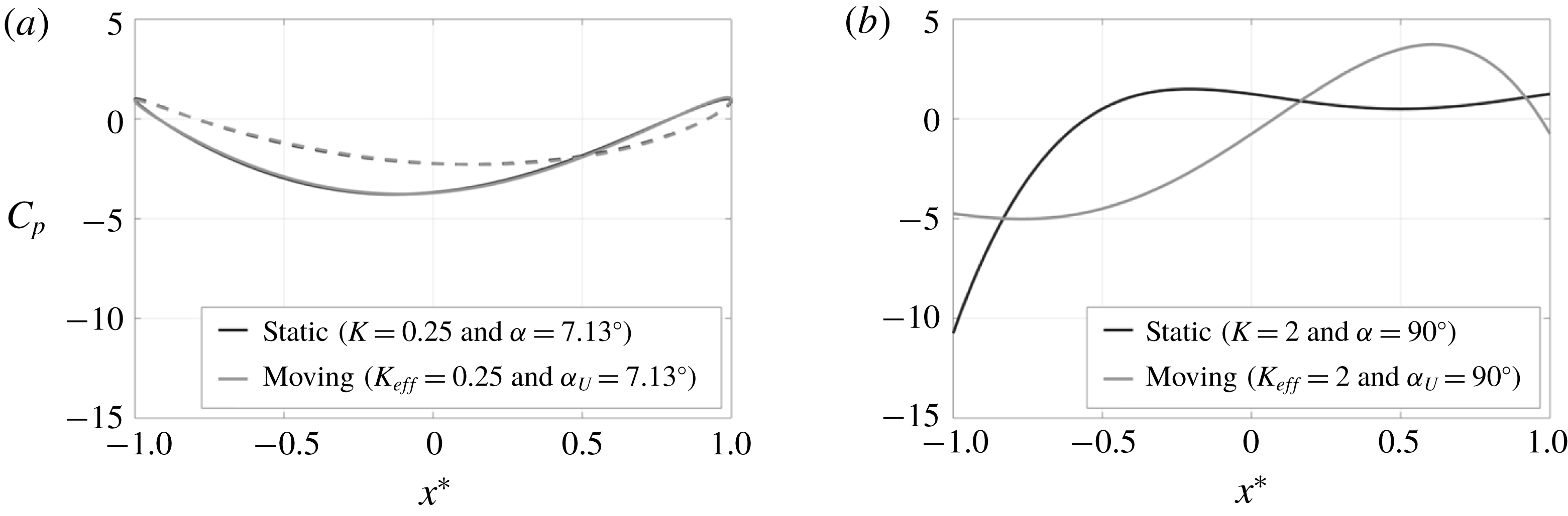
(figure 9). Moreover, considering the corresponding
 $C_{p}$
distribution (figure 13
a), it is evident that both flows have practically identical surface pressure distribution. This is to be contrasted, for example, with the case when both
 $K_{eff}$
and
 $\unicode[STIX]{x1D6FC}_{U}$
reach their maximum values at shear centre (
 $Y_{0}^{\ast }=0$
), and both QU and QS conditions are not expected to hold. The
 $C_{p}$
profile for the latter case is shown in figure 13(b), which demonstrates the drastic difference in the
 $C_{p}$
distribution between the two flows.
Comparison between the streamlines around the moving cylinder (a) when located at
 $Y_{o}^{\ast }=8$
(
 $K_{eff,max}=2$
) with those around a static cylinder, (b) having the same approach stream’s non-dimensional shear rate and angle of incidence as the instantaneous
 $K_{eff}$
and
 $\unicode[STIX]{x1D6FC}_{U}$
for the moving cylinder. Broken lines show the streamlines if the cylinder were absent.

Comparison of the surface
 $C_{p}$
distributions of the moving- and static-cylinder cases in the limit of (a) low and (b) high
 $K_{eff}$
and
 $\unicode[STIX]{x1D6FC}_{U}$
values. Solid and broken lines, respectively, depict the
 $C_{p}$
distribution on the upper and lower surface. At the shear centre (b), the solid and broken lines are indistinguishable since the pressure distribution is symmetric between the top and bottom surfaces.

Since the force expressions for the moving and the static cylinders are serendipitously identical regardless of the problem parameters, force cannot be used in characterizing QUS limits. As an alternative, the difference in the
 $C_{p}$
distribution (
 $\unicode[STIX]{x0394}C_{p}$
) may be used to quantify the deviation from QUS flow conditions. Here, it is important to emphasize the distinction between ‘quasi-steadiness’, ‘quasi-uniformity’ and ‘quasi-steadiness and quasi-uniformity’. Referring to figure 3, since only the uniform flow is unsteady (with its magnitude and angle of incidence changing with time), a QS version of this flow involves replacing the unsteady uniform flow with a steady equivalent while maintaining the same centred-shear flow component. The
 $C_{p}$
for this flow is obtained from that of the static cylinder (B 1) by replacing
 $K$
with
 $K_{eff}$
, and
 $\unicode[STIX]{x1D703}$
with
 $\unicode[STIX]{x1D703}-\unicode[STIX]{x1D6FC}_{U}$
in the uniform-flow term only. Subtracting the resulting
 $C_{p}$
from that of the moving cylinder (2.20),
 $$\begin{eqnarray}\displaystyle \unicode[STIX]{x0394}C_{p,QS}=C_{p}-C_{p,QS}=2K_{eff}\sin (\unicode[STIX]{x1D6FC}_{U})\cos (\unicode[STIX]{x1D703})=2\dot{U}_{o}^{+}\cos (\unicode[STIX]{x1D703}). & & \displaystyle\end{eqnarray}$$
As reasoned using (3.17), (3.18) explicitly shows that as
 $\dot{U}_{o}^{+}\rightarrow 0$
, the pressure distribution becomes the same as that of the static cylinder; i.e. the flow becomes quasi-steady.
In practice, the quasi-steady problem is not of direct interest by itself since connecting the static- and the moving-cylinder flows is only useful if one rotates the entire approach stream; i.e. both the uniform- and the shear-flow components. However, as discussed in connection with equation (2.7), in the presence of shear, it is not possible to define a unique angle of incidence of the approach stream, except in the quasi-uniform flow limit. Thus, rotating the entire approach stream by
 $\unicode[STIX]{x1D6FC}_{U}$
and replacing the uniform flow component with a steady equivalent, implies both quasi-uniformity and quasi-steadiness. With this important proviso,
 $C_{p}$
for QUS conditions is obtained by replacing
 $K$
with
 $K_{eff}$
and
 $\unicode[STIX]{x1D703}$
with
 $\unicode[STIX]{x1D703}-\unicode[STIX]{x1D6FC}_{U}$
in all terms of equation (B 1) of the static cylinder, and the result is subtracted from the complete pressure distribution (2.20) to produce the following:
 $$\begin{eqnarray}\displaystyle \unicode[STIX]{x0394}C_{p,QUS} & = & \displaystyle C_{p}-C_{p,QUS}=2K_{eff}\sin (\unicode[STIX]{x1D6FC}_{U})\cos (\unicode[STIX]{x1D703})\nonumber\\ \displaystyle & & \displaystyle +\,2K_{eff}\sin (\unicode[STIX]{x1D703}-\unicode[STIX]{x1D6FC}_{U})[\cos (2\unicode[STIX]{x1D703})-\cos (2(\unicode[STIX]{x1D703}-\unicode[STIX]{x1D6FC}_{U}))]\nonumber\\ \displaystyle & & \displaystyle +\,\frac{1}{4}K_{eff}^{2}\big\{[\cos (2\unicode[STIX]{x1D703})-\cos (2(\unicode[STIX]{x1D703}-\unicode[STIX]{x1D6FC}_{U}))]\nonumber\\ \displaystyle & & \displaystyle -[\cos ^{2}(2\unicode[STIX]{x1D703})-\cos ^{2}(2(\unicode[STIX]{x1D703}-\unicode[STIX]{x1D6FC}_{U}))]\big\}.\end{eqnarray}$$
The last equation can be rewritten as a Fourier series in
 $\unicode[STIX]{x1D703}$
, which after maintaining the terms organization based on the exponent of
 $K_{eff}$
, yields,
 $$\begin{eqnarray}\displaystyle \unicode[STIX]{x0394}C_{p,QUS} & = & \displaystyle 2K_{eff}\sin (\unicode[STIX]{x1D6FC}_{U})\cos (3\unicode[STIX]{x1D703}-2\unicode[STIX]{x1D6FC}_{U})\nonumber\\ \displaystyle & & \displaystyle -\,\frac{1}{4}K_{eff}^{2}\left[2\sin (\unicode[STIX]{x1D6FC}_{U})\sin \left(2\unicode[STIX]{x1D703}-\unicode[STIX]{x1D6FC}_{U}\right)-\sin (2\unicode[STIX]{x1D6FC}_{U})\sin (4\unicode[STIX]{x1D703}-2\unicode[STIX]{x1D6FC}_{U})\right].\end{eqnarray}$$
If the flow is quasi-uniform,
 $K_{eff}\rightarrow 0$
and the quadratic term in equation (3.20) may then be neglected, leading to the following:
 $$\begin{eqnarray}\displaystyle \unicode[STIX]{x0394}C_{p,QU}=2K_{eff}\sin (\unicode[STIX]{x1D6FC}_{U})\cos (3\unicode[STIX]{x1D703}-2\unicode[STIX]{x1D6FC}_{U})=2\dot{U}_{o}^{+}\cos (3\unicode[STIX]{x1D703}-2\unicode[STIX]{x1D6FC}_{U}). & & \displaystyle\end{eqnarray}$$
It is interesting to see that the maximum deviation
 $\unicode[STIX]{x0394}C_{p,max}$
between the moving cylinder and the QS (3.18) and QU (3.21) cases is the same:
 $\unicode[STIX]{x0394}C_{p,max}=2\dot{U}_{o}^{+}$
. This demonstrates that when the flow is quasi-uniform, it is also quasi-steady, and vice versa. In other words, though fundamentally, these two concepts describe different physics (uniformity in space versus invariance with time), it is not possible to achieve one of these conditions without the other in this flow problem. Accordingly, for an object translating across a uniform shear zone, the only possible simplification is that of a quasi-uniform and quasi-steady flow.
The maximum of equation (3.19) is plotted versus
 $\dot{U}_{o}^{+}$
for two different values of
 $K_{eff,max}$
in figure 14. It is helpful to note that for a given
 $K_{eff,max}$
, the parameters
 $K_{eff}$
and
 $\dot{U}_{o}^{+}$
change from zero to
 $K_{eff,max}$
as the cylinder translates from
 $+\infty$
to
 $Y_{o}^{\ast }=0$
(see (2.14), (2.15) and (3.17)). Thus, the curve corresponding to
 $K_{eff,max}=0.1$
is only plotted up to
 $\dot{U}_{o}^{+}=0.1$
in figure 14. As seen from the figure, the maximum deviation from the QUS approximation increases monotonically with the shear rate
 $K_{eff,max}$
for the same
 $\dot{U}_{o}^{+}$
; i.e. the deviation is not a function of
 $\dot{U}_{o}^{+}$
only. However, as
 $\unicode[STIX]{x0394}C_{p,max}\rightarrow 0$
, the results in figure 14 converge towards the quasi-uniform (or quasi-steady) flow behaviour where
 $\unicode[STIX]{x0394}C_{p,max}=2\dot{U}_{o}^{+}$
. Using this equation, and assuming, for example, that
 $\unicode[STIX]{x0394}C_{p,max}$
of 0.05 is a sufficiently negligible deviation, then
 $\dot{U}_{o}^{+}$
should be less than 0.025 for QUS to be a reasonable approximation of the flow. Moreover, if the cylinder velocity is sufficiently small, then
 $\sin (\unicode[STIX]{x1D6FC}_{U})\approx V_{r}$
, leading to a corresponding QUS flow criterion expressed directly in terms of the effective shear rate and the velocity ratio:
 $K_{eff}V_{r}<0.025$
. This value, though based on an arbitrary threshold, helps to give a physical sense of the order of magnitude of
 $\dot{U}_{o}^{+}$
over which quasi-uniformity and quasi-steadiness is a reasonable approximation.
Maximum deviation in the surface-pressure-coefficient distribution of the moving cylinder from that arising under quasi-uniform and quasi-steady flow conditions.

4 Conclusions
In this paper, we find the inviscid solution of the flow around a circular cylinder traversing at constant velocity across an infinitely wide, uniform-shear free stream. The solution is obtained in a Galilean frame of reference, fixed to the translating cylinder. With this transformation, the approach stream becomes unsteady, exhibiting a change in the stream’s reference velocity at the cross-stream location of the cylinder’s centre.
The results show that, far from the cylinder, the undisturbed approach flow has parabolic streamlines, which makes it impossible to define an angle of incidence for the free stream; as commonly done when a cylinder traverses across uniform flow. As the cylinder traverses from infinity, on the high-speed side, towards the shear centre (where the free stream velocity is zero), the magnitude of the force acting on the cylinder increases monotonically. The corresponding force direction changes from being normal to the approach stream (in the lift direction) to being against the stream (in the thrust direction). These variations cause a non-monotonic change in lift, with a maximum observed during the motion history, while the thrust increases monotonically during the cylinder’s motion. The lift force is found to be generated by a shearing mechanism, exactly similar to that on a static cylinder in uniform-shear flow (Tsien Reference Tsien1943). In contrast, the thrust is produced by the perceived deceleration of the free stream relative to the cylinder, as the latter traverses in a direction of decreasing free stream velocity.
An effort is made to connect the moving-cylinder solution to the static-cylinder counterpart. This is motivated by the equivalent problem in uniform free stream, where the moving-cylinder solution can be obtained directly from the static-cylinder case with a simple change in the magnitude and incidence angle of the free stream velocity. To connect the moving and the static cylinder problems, a new terminology of ‘quasi-uniform’ flow is introduced. This idea, which describes the flow state in the limit of weak shear, is the spatial equivalent of the temporal concept of QS flow. It is found that, in the present flow problem, quasi-uniformity and quasi-steadiness are not independent; i.e. when the flow is QU it is also QS and vice versa. In the limit of this QUS flow condition, a physically meaningful free stream incidence angle
 $\unicode[STIX]{x1D6FC}$
could be defined for the moving cylinder, and the effect of flow unsteadiness is solely determined by a single parameter
 $(\dot{U}_{o}^{+})$
characterizing the non-dimensional rate of change of the approach stream velocity as the cylinder traverses across the shear flow. As
 $\dot{U}_{o}^{+}\rightarrow 0$
, the flow is QUS, and the moving-cylinder problem approaches that of a static cylinder in uniform-shear flow with a shear rate equal to the instantaneous non-dimensional shear rate
 $K_{eff}$
of the moving cylinder, and an angle of incidence determined from
 $\tan ^{-1}(V_{r})$
; where
 $V_{r}$
is the instantaneous cylinder-to-reference velocity ratio. For small
 $V_{r}$
,
 $\dot{U}_{o}^{+}$
is approximately equal to
 $K_{eff}V_{r}$
.
A surprising result is that, notwithstanding the differences between the static- and moving-cylinder problems, the force magnitude and direction is found to be the same in both cases, when the static-cylinder’s non-dimensional shear rate is set to
 $K_{eff}$
, and the approach-stream’s angle of incidence is set to
 $\tan ^{-1}(V_{r})$
. This finding holds regardless of the values of
 $K_{eff}$
and
 $V_{r}$
. The force equality is achieved despite differences in the surface pressure distribution since the change in the latter occurs without change in its integrated effect around the cylinder. Further analysis shows that the streamwise component of the force acting on the moving cylinder has a different physical nature than that acting on the static cylinder. Specifically, this component is produced via an inertia mechanism for the former, in contrast to a shearing effect for the latter. It is shown that the inertia mechanism for the specific situation considered, where the shear is uniform and the cylinder’s velocity is constant, produces a similar force-component magnitude. It is hypothesized that this result is serendipitous, and will likely not hold for more general free stream shear profiles and/or cylinder motion. Moreover, in real flow problems, where viscous effects are present, the difference in surface pressure distribution would lead to different boundary layer development history and separation characteristics, which should lead to force inequality.
Beyond addressing a fundamental flow problem; i.e. a circular cylinder traversing across uniform shear region, the present study lays the theoretical framework for analysing moving objects in shear flows. Future effort will extend the present work to an airfoil moving across uniform shear.
Acknowledgements
The authors would like to acknowledge the support of this work by ONR grant number N00014-16-2760. The views and conclusions contained in this document are those of the authors and should not be interpreted as representing the official policies, either expressed or implied, of ONR or the US Government.
Appendix A.
Starting with making (2.17) non-dimensional,
 $$\begin{eqnarray}\displaystyle \displaystyle C_{p} & = & \displaystyle \frac{p_{2}-p_{1}}{\frac{1}{2}\unicode[STIX]{x1D70C}U_{o,eff}^{2}}=\frac{1}{\frac{1}{2}U_{o,eff}^{2}}(Q_{1}^{2}-Q_{2}^{2})+\frac{1}{\frac{1}{2}U_{o,eff}^{2}}\int _{1}^{2}\!\left[\frac{U_{o,eff}(d/2)}{(d/2)^{2}}\unicode[STIX]{x1D6FB}^{\ast 2}\unicode[STIX]{x1D713}^{\ast }\right]\!\left[U_{o,eff}\left(\frac{d}{2}\right)\,\text{d}\unicode[STIX]{x1D713}^{\ast }\right]\nonumber\\ \displaystyle & & \displaystyle -\,\frac{1}{\frac{1}{2}U_{o,eff}^{2}}\int _{1}^{2}\frac{\unicode[STIX]{x2202}Q_{s}}{\unicode[STIX]{x2202}t}\,\text{d}s=0,\end{eqnarray}$$
which simplifies to
 $$\begin{eqnarray}\displaystyle C_{p}=\frac{p_{2}-p_{1}}{\frac{1}{2}\unicode[STIX]{x1D70C}U_{o,eff}^{2}}=(Q_{1}^{\ast 2}-Q_{2}^{\ast 2})+2\int _{1}^{2}\unicode[STIX]{x1D6FB}^{\ast 2}\unicode[STIX]{x1D713}^{\ast }\,\text{d}\unicode[STIX]{x1D713}^{\ast }-\frac{1}{\frac{1}{2}U_{o,eff}^{2}}\int _{1}^{2}\frac{\unicode[STIX]{x2202}Q_{s}}{\unicode[STIX]{x2202}t}\,\text{d}s. & & \displaystyle\end{eqnarray}$$
Considering the integrand in the third term on the right-hand side by itself
 $$\begin{eqnarray}\displaystyle & \displaystyle \frac{\unicode[STIX]{x2202}Q_{s}}{\unicode[STIX]{x2202}t}=\frac{\unicode[STIX]{x2202}(U_{o,eff}Q_{s}^{\ast })}{\unicode[STIX]{x2202}t}=U_{o,eff}\frac{\unicode[STIX]{x2202}Q_{s}^{\ast }}{\unicode[STIX]{x2202}t}+Q_{s}^{\ast }\frac{\text{d}U_{o,eff}}{\text{d}t}=U_{o,eff}\frac{\unicode[STIX]{x2202}Q_{s}^{\ast }}{\unicode[STIX]{x2202}t}+Q_{s}^{\ast }\frac{\text{d}}{\text{d}t}\!\!\left(\sqrt{U_{o}^{2}+V_{o}^{2}}\right)\!,\quad & \displaystyle\end{eqnarray}$$
 $$\begin{eqnarray}\displaystyle & \displaystyle \frac{\unicode[STIX]{x2202}Q_{s}}{\unicode[STIX]{x2202}t}=U_{o,eff}\frac{\unicode[STIX]{x2202}Q_{s}^{\ast }}{\unicode[STIX]{x2202}t}+Q_{s}^{\ast }\frac{1}{2}(U_{o}^{2}+V_{o}^{2})^{-1/2}2U_{o}\frac{\text{d}U_{o}}{\text{d}t}. & \displaystyle\end{eqnarray}$$
Using
 $\text{d}U_{o}/\text{d}t=-mV_{o}$
, leads to
 $$\begin{eqnarray}\displaystyle & \displaystyle \frac{\unicode[STIX]{x2202}Q_{s}}{\unicode[STIX]{x2202}t}=U_{o,eff}\frac{\unicode[STIX]{x2202}Q_{s}^{\ast }}{\unicode[STIX]{x2202}t}-Q_{s}^{\ast }\frac{U_{o}}{(U_{o}^{2}+V_{o}^{2})^{1/2}}mV_{o}. & \displaystyle\end{eqnarray}$$
Using
 $V_{o}/(U_{o}^{2}+V_{o}^{2})^{1/2}=V_{o}/U_{o,eff}=\sin (\unicode[STIX]{x1D6FC}_{U})$
,
 $$\begin{eqnarray}\displaystyle & \displaystyle \frac{\unicode[STIX]{x2202}Q_{s}}{\unicode[STIX]{x2202}t}=U_{o,eff}\frac{\unicode[STIX]{x2202}Q_{s}^{\ast }}{\unicode[STIX]{x2202}t}-mU_{o}\sin (\unicode[STIX]{x1D6FC}_{U})Q_{s}^{\ast }. & \displaystyle\end{eqnarray}$$
Substituting (A 6) in (A 2) and normalizing
 $s$
using
 $d/2$
,
 $$\begin{eqnarray}\displaystyle \displaystyle C_{p} & = & \displaystyle \frac{p_{2}-p_{1}}{\frac{1}{2}\unicode[STIX]{x1D70C}U_{o,eff}^{2}}=(Q_{1}^{\ast 2}-Q_{2}^{\ast 2})+2\int _{1}^{2}\unicode[STIX]{x1D6FB}^{\ast 2}\unicode[STIX]{x1D713}^{\ast }d\unicode[STIX]{x1D713}^{\ast }-\frac{1}{\frac{1}{2}U_{o,eff}^{2}}\nonumber\\ \displaystyle & & \displaystyle \int _{1}^{2}\left(U_{o,eff}\frac{\unicode[STIX]{x2202}Q_{s}^{\ast }}{\unicode[STIX]{x2202}t}-mU_{o}\sin (\unicode[STIX]{x1D6FC}_{U})Q_{s}^{\ast }\right)\left(\frac{d}{2}\text{d}s^{\ast }\right),\end{eqnarray}$$
which, upon recognizing that
 $K_{eff}=md/U_{o,eff}$
, and
 $U_{o}/U_{eff}=\cos (\unicode[STIX]{x1D6FC}_{U})$
, leads to the form of (2.18),
 $$\begin{eqnarray}\displaystyle \displaystyle C_{p} & = & \displaystyle \frac{p_{2}-p_{1}}{\frac{1}{2}\unicode[STIX]{x1D70C}U_{o,eff}^{2}}=(Q_{1}^{\ast 2}-Q_{2}^{\ast 2})+2\int _{1}^{2}\unicode[STIX]{x1D6FB}^{\ast 2}\unicode[STIX]{x1D713}^{\ast }\,\text{d}\unicode[STIX]{x1D713}^{\ast }-\frac{d}{U_{o,eff}}\int _{1}^{2}\frac{\unicode[STIX]{x2202}Q_{s}^{\ast }}{\unicode[STIX]{x2202}t}\,\text{d}s^{\ast }\nonumber\\ \displaystyle & & \displaystyle +\,K_{eff}\cos (\unicode[STIX]{x1D6FC}_{U})\sin (\unicode[STIX]{x1D6FC}_{U})\int _{1}^{2}Q_{s}^{\ast }\,\text{d}s^{\ast }.\end{eqnarray}$$
Appendix B.
One useful check on the form of equation (2.20) is to simplify it to the form for the static cylinder in shear. This result has not been derived elsewhere, including in Tsien (Reference Tsien1943), who obtained the lift force on the cylinder using a control volume approach, rather than using the surface pressure distribution. To get the pressure coefficient for the static cylinder, let
 $\unicode[STIX]{x1D6FC}_{U}\rightarrow 0$
(i.e.
 $V_{o}=0$
),
 $U_{o,eff}\rightarrow U_{o}$
and
 $K_{eff}\rightarrow K$
in (2.20), leading to,
 $$\begin{eqnarray}\displaystyle \displaystyle C_{p}(\unicode[STIX]{x1D703}) & = & \displaystyle \frac{p(\unicode[STIX]{x1D703})-p_{\infty }}{\frac{1}{2}\unicode[STIX]{x1D70C}U_{o}^{2}}=[1-4\,\sin ^{2}(\unicode[STIX]{x1D703})]-2K\sin (\unicode[STIX]{x1D703})\left[\frac{1}{2}-\cos (2\unicode[STIX]{x1D703})\right]\nonumber\\ \displaystyle & & \displaystyle +\,\frac{K^{2}}{16}[1+4\cos (2\unicode[STIX]{x1D703})-4\cos ^{2}(2\unicode[STIX]{x1D703})].\end{eqnarray}$$
The analytical form (B 1), which also correctly reduces to the well known uniform-approach-flow form in the limit
 $K\rightarrow 0$
, may be verified by re-deriving (B 1) using the usual approach of choosing points 1 and 2 in (2.18) along a streamline for Tsien’s steady problem. In this case, the stagnation streamline is selected for evaluating (2.18) with point 1 far upstream along the streamline (denoted as
 $s\infty$
), and point 2 is on the surface of the cylinder. The combination of a streamline integration path and flow steadiness eliminates the integral terms in (2.18), yielding the simple form,
 $$\begin{eqnarray}\displaystyle & \displaystyle C_{p}(\unicode[STIX]{x1D703})=\frac{p(\unicode[STIX]{x1D703})-p_{\infty }}{\frac{1}{2}\unicode[STIX]{x1D70C}U_{o}^{2}}=\left(U_{s\infty }^{\ast 2}-U_{\unicode[STIX]{x1D703}}^{\ast 2}\right), & \displaystyle\end{eqnarray}$$
where,
 $U_{s\infty }^{\ast }$
is the approach stream velocity on the stagnation streamline far upstream of the cylinder (i.e.
 $x_{1}^{\ast }\rightarrow -\infty$
) and
 $U_{\unicode[STIX]{x1D703}}^{\ast }$
is the azimuthal slip velocity on the cylinder surface.
To obtain
 $U_{s\infty }^{\ast }$
, we consider the asymptotic cross-stream coordinate
 $y_{s\infty }^{\ast }$
of the upper stagnation streamline far upstream from the cylinder. As seen in figure 6, this coordinate increases in the positive direction with increasing
 $K$
. To find
 $y_{s\infty }^{\ast }$
, the stagnation streamline stream function magnitude is found by evaluating (2.1) on the cylinder surface. Once this value is known, (2.1) is evaluated in the limit
 $r^{\ast }\rightarrow \infty$
, yielding,
 $$\begin{eqnarray}\displaystyle & \displaystyle y_{s\infty }^{\ast }=-\frac{2}{K}\left(1-\sqrt{1+\frac{K^{2}}{8}}\right). & \displaystyle\end{eqnarray}$$
Substitution of (B 3) in the approach stream linear velocity profile, gives the approach velocity on the stagnation streamline,
 $$\begin{eqnarray}\displaystyle U_{s\infty }^{\ast }=\sqrt{1+\frac{K^{2}}{8}}. & & \displaystyle\end{eqnarray}$$
Also, using (2.5) with
 $r^{\ast }=1$
to obtain
 $U_{\unicode[STIX]{x1D703}}^{\ast }$
on the cylinder’s surface,
 $$\begin{eqnarray}\displaystyle U_{\unicode[STIX]{x1D703}}^{\ast 2}=\left[2\sin (\unicode[STIX]{x1D703})+\frac{K}{2}\left(\sin ^{2}(\unicode[STIX]{x1D703})-\frac{1}{2}\cos (2\unicode[STIX]{x1D703})\right)\right]^{2}. & & \displaystyle\end{eqnarray}$$
Substituting (B 4) and (B 5) in (B 2) gives the same form as (B 1).