1 Introduction
The flow of a Newtonian fluid over a smooth-wall cylinder is interesting not only for its wide engineering application but also because it is a canonical problem in bluff-body aerodynamics. Research on flow over a cylinder has been active since the early twentieth century, when the boundary-layer theory was established. Interest in this flow intensified during the 1961–1990 period, stimulated by the signature experiment by Roshko (Reference Roshko1961), which demonstrated the reappearance of vortex shedding at Reynolds numbers larger than
 $Re_{D}=U_{\infty }\,D/\unicode[STIX]{x1D708}=3\times 10^{6}$
, with
 $D$
the diameter of the cylinder,
 $U_{\infty }$
the free-stream flow speed and
 $\unicode[STIX]{x1D708}$
the constant kinematic fluid viscosity. In these two periods, several well-conceived experiments contributed further to our understanding of cylinder flow. However, as pointed out in reviews by Roshko (Reference Roshko1993) and Williamson (Reference Williamson1996), the cumulative experimental results have yet to provide a consistent general theory of cylinder flow at very large Reynolds numbers. Even for the drag coefficient
 $C_{D}$
, the experimental data collected by Cantwell & Coles (Reference Cantwell and Coles1983) at high Reynolds number show considerable scatter over, for example, the
 $Re_{D}$
range typical of the drag crisis.
Flow over a cylinder is known to exhibit an interesting range of physical phenomena. With increasing
 $Re_{D}$
, the flow develops from a steady and stable state with a closed wake to two-dimensional and then three-dimensional unsteady flow following wake transition, shear-layer transition and possibly boundary-layer transition. Beyond a critical Reynolds number, in the range
 $Re_{D}=1000{-}2000$
, the flow is observed to first become turbulent, due to incipient Kelvin–Helmholtz instability of the two shear layers separating from the cylinder surface. Prasad & Williamson (Reference Prasad and Williamson1997) found that the shear-layer instability is affected by the primary vortex shedding. In their results, instability begins at
 $Re_{D}\approx 1200$
for parallel primary shedding and
 $Re_{D}\approx 2600$
for oblique primary shedding. Above this critical transition region, turbulence in the wake flow increases in strength and moves upstream with increasing Reynolds number. A general tendency for shear-layer transition can be observed for increasing
 $Re_{D}$
, accompanied by increasing drag coefficient
 $C_{D}$
and shrinking of the recirculation length. Weidman (Reference Weidman1968) studied the flow in this
 $Re_{D}$
range, finding that the cylinder-surface pressure minima between
 $Re_{D}=10^{4}$
and
 $10^{5}$
show little variation with
 $Re_{D}$
.
When, with increasing
 $Re_{D}$
, the shear-layer turbulence approaches the cylinder surface, transition takes place on the top of a small separation bubble. This produces a reattached turbulent boundary layer, which in turn leads to deferred large-scale separation around the cylinder surface. Owing to the resulting contraction of the portion of the cylinder surface over which the boundary layer has suffered large-scale separation, a decrease of
 $C_{D}$
then occurs over a relatively small band of
 $Re_{D}$
. This is known as the ‘drag crisis’. In the literature, the terms sub-critical and super-critical refer to
 $Re_{D}$
below and above the drag-crisis band respectively.
Experimental evidence indicates some irregular phenomena in the drag-crisis regime. Asymmetric flow, where one-sided transition occurs on the separation bubble, was observed by Bearman (Reference Bearman1969) and Achenbach & Heinecke (Reference Achenbach and Heinecke1981), and studied in detail by Schewe (Reference Schewe1983), where one-sided bubble and bifurcation transitions were confirmed. Schewe (Reference Schewe1983) reported that the asymmetric state is stable for a small range of
 $Re_{D}$
, and that only for sufficiently high
 $Re_{D}$
do perturbations on both sides of the cylinder stimulate a nearly symmetric state with two-sided transition. If
 $Re_{D}$
is increased past the drag crisis, direct boundary-layer transition is observed and the flow is said to move into the trans-critical regime. Here,
 $C_{D}$
again increases with
 $Re_{D}$
. One well-known difficulty with experiments is that cylinder flow at high Reynolds number is sensitive to many effects, including wind tunnel blockage, surface roughness, free-stream turbulence levels and the presence of either controlled or uncontrolled flow perturbations. It can be plausibly hypothesized that, in principle, numerical simulation can avoid some aspects of experimental uncertainty and thus could provide constructive insights elucidating the physics of flow over a cylinder.
Numerical simulation has demonstrated both the potential and capability for accurate calculation of the Reynolds-number dependence of turbulent flows, including flow over bluff bodies. As for many wall-bounded turbulent flows, the numerical simulation of cylinder flow can be separated into three main categories. The most accurate approach is direct numerical simulation (DNS), for which much work has focused on
 $Re_{D}=3.9\times 10^{3}$
; e.g. Beaudan & Moin (Reference Beaudan and Moin1994). Important issues have included domain influence, the particular numerical method, and boundary conditions; see, for example, Kravchenko & Moin (Reference Kravchenko and Moin2000) and Ma, Karamanos & Karniadakis (Reference Ma, Karamanos and Karniadakis2000). Direct numerical simulation, which is restricted by its rapidly increasing computational requirement with increasing
 $Re_{D}$
, has been extended to
 $Re_{D}=10^{4}$
by Dong et al. (Reference Dong, Karniadakis, Ekmekci and Rockwell2006), but this remains well below the drag-crisis regime.
At larger
 $Re_{D}$
, either wall-resolved or some form of wall-modelled large-eddy simulation (LES), such as that of Catalano et al. (Reference Catalano, Wang, Iaccarino and Moin2003) at
 $Re_{D}=3.6\times 10^{5}$
, or detached-eddy simulation (DES) (Travin et al.
Reference Travin, Shur, Strelets and Spalart1999) at
 $Re_{D}=3\times 10^{6}$
is required in order to make contact with high-Reynolds-number experiments. With a few exceptions, such as Travin et al. (Reference Travin, Shur, Strelets and Spalart1999), there has been little emphasis on numerical simulation in the gap separating these values of
 $Re_{D}$
and the range presently accessible to DNS. The major aims of the present work are to perform LES over a range of
 $Re_{D}$
that bridges this gap, with particular focus on the behaviour of the skin-friction,
 $C_{f}$
, distribution along the cylinder surface insofar as this is related to the mechanics of separation, and the near-wall properties of the separated flow. As will be seen in the present study, at least up to
 $Re_{D}=8.5\times 10^{5}$
in the super-critical regime, the cylinder boundary layer remains either laminar or else in transition to turbulence at moderate
 $Re_{\unicode[STIX]{x1D70F}}=\unicode[STIX]{x1D6FF}\,u_{\unicode[STIX]{x1D70F}}/\unicode[STIX]{x1D708}$
, where
 $\unicode[STIX]{x1D6FF}$
is a local boundary-layer thickness and
 $u_{\unicode[STIX]{x1D70F}}$
is some measure of local surface skin-friction velocity. Here, it is reasonable to expect that a wall-modelled approach may not be needed and that wall-resolved LES is appropriate.
In wall-resolved LES, subgrid-scale (SGS) modelling is applied to the outer flow away from the wall, while the near-wall flow is resolved at least in the wall-normal direction. While, for the present cylinder flow, wall-resolved LES will be adequate for
 $Re_{D}$
in the super-critical and up to the early trans-critical regime, it may not be practical for
 $Re_{D}=O(10^{7}{-}10^{8})$
and larger. An example of the wall-resolved approach is given by Lehmkuhl et al. (Reference Lehmkuhl, Rodríguez, Borrell, Chiva and Oliva2014), who implemented wall-resolved LES from
 $2.5\times 10^{5}$
to
 $6.5\times 10^{5}$
, with emphasis on the pressure distribution during vortex shedding. They reported results on separation behaviour but showed limited
 $C_{f}$
distributions.
We report on wall-resolved LES of flow past a smooth-wall cylinder for
 $Re_{D}$
in the range from
 $Re_{D}=3.9\times 10^{3}$
to
 $Re_{D}=8.5\times 10^{5}$
. In what follows, brief descriptions of the numerical code and the SGS model used are given in § 2. The skin-friction vector field, which is the main topic of the present study, is then defined, with three different averaged forms and two different ways to compute the skin friction from LES data. Results from wall-resolved LES over an
 $Re_{D}$
range in the sub-critical regime, beginning from
 $Re_{D}=3.9\times 10^{3}$
, are described in § 3, and results are compared with skin-friction data from experiments by Son & Hanratty (Reference Son and Hanratty1969). Several LES in the super-critical regime are discussed in § 4, where comparison with corresponding experiments is made. Other properties of the flow are discussed, including the boundary-layer development in § 5, the behaviour of separation in § 6 and the patterns of the surface skin-friction vector fields in § 7. Conclusions are given in § 8.
2 Numerical method and physical model
We denote by
 $(x_{1},x_{2},x_{3})$
or
 $(x,y,z)$
Cartesian coordinates with corresponding velocity components (
 $u_{x},u_{y},u_{z}$
);
 $(\unicode[STIX]{x1D709}_{1},\unicode[STIX]{x1D709}_{2},\unicode[STIX]{x1D709}_{3})$
or
 $(\unicode[STIX]{x1D709},y,\unicode[STIX]{x1D702})$
are curvilinear coordinates with velocity components (
 $u^{\unicode[STIX]{x1D709}},u^{y},u^{\unicode[STIX]{x1D702}}$
). We also employ cylindrical coordinates
 $(r,\unicode[STIX]{x1D703},y)$
with
 $-\unicode[STIX]{x03C0}<\unicode[STIX]{x1D703}\leqslant \unicode[STIX]{x03C0}$
, with velocity components (
 $u_{r},u_{\unicode[STIX]{x1D703}},u_{y}$
), with
 $x=-r\cos \unicode[STIX]{x1D703}$
,
 $z=r\sin \unicode[STIX]{x1D703}$
and with
 $y$
the spanwise direction.
We consider flow past a cylinder of dimensionless diameter
 $D=1$
. In
 $(r,\unicode[STIX]{x1D703},y)$
coordinates, the cylinder axis lies along the
 $y$
-axis and the cylinder surface is
 $r=0.5$
. The flow at infinity is uniform in the positive
 $x$
direction with speed
 $U_{\infty }=1$
. Along the surface of the cylinder cut by the
 $x{-}z$
-plane,
 $\unicode[STIX]{x1D703}=0$
at the nominal windward stagnation point and
 $\unicode[STIX]{x1D703}=\unicode[STIX]{x03C0}$
at the nominal rear stagnation point. The kinematic viscosity is
 $\unicode[STIX]{x1D708}$
and
 $Re_{D}=U_{\infty }\,D/\unicode[STIX]{x1D708}$
.
2.1 Numerical method
The governing equations for LES are obtained by formally filtering the incompressible Navier–Stokes equations with filter size or cutoff length
 $\unicode[STIX]{x1D6E5}_{c}$
, which is here related directly to the mesh resolution. Utilizing a collocated mesh strategy in a general curvilinear coordinate (Zang, Street & Koseff Reference Zang, Street and Koseff1994), the filtered governing equations in conservation-law form can be written as
 $$\begin{eqnarray}\frac{\unicode[STIX]{x2202}U^{m}}{\unicode[STIX]{x2202}\unicode[STIX]{x1D709}^{m}}=0,\quad \frac{J^{-1}\unicode[STIX]{x2202}\tilde{u_{i}}}{\unicode[STIX]{x2202}t}+\frac{\unicode[STIX]{x2202}F_{i}^{m}}{\unicode[STIX]{x2202}\unicode[STIX]{x1D709}^{m}}=0,\end{eqnarray}$$
where
 $U^{m}$
and
 $F^{m}$
are given as
 $$\begin{eqnarray}U^{m}=J^{-1}\frac{\unicode[STIX]{x2202}\unicode[STIX]{x1D709}^{m}}{\unicode[STIX]{x2202}x_{i}}\widetilde{u_{i}}\quad \text{and}\quad F_{i}^{m}=U^{m}\widetilde{u_{i}}+J^{-1}\frac{\unicode[STIX]{x2202}\unicode[STIX]{x1D709}^{m}}{\unicode[STIX]{x2202}x_{j}}\unicode[STIX]{x1D61B}_{ij}+J^{-1}\frac{\unicode[STIX]{x2202}\unicode[STIX]{x1D709}^{m}}{\unicode[STIX]{x2202}x_{i}}\tilde{p}-\unicode[STIX]{x1D708}\unicode[STIX]{x1D60E}^{mn}\frac{\unicode[STIX]{x2202}\widetilde{u_{i}}}{\unicode[STIX]{x2202}\unicode[STIX]{x1D709}^{n}}\end{eqnarray}$$
respectively. The SGS tensor
 $\unicode[STIX]{x1D61B}_{ij}=\widetilde{u_{i}u_{j}}-\widetilde{u_{i}}\widetilde{u_{j}}$
is the unresolved nonlinear term that is modelled in LES. Here,
 $J^{-1}$
is the inverse of the Jacobian and
 $\unicode[STIX]{x1D60E}^{mn}$
is the mesh skewness tensor. These mesh properties are defined as
 $$\begin{eqnarray}J^{-1}=\det \left(\frac{\unicode[STIX]{x2202}x_{i}}{\unicode[STIX]{x2202}\unicode[STIX]{x1D709}^{j}}\right),\quad \unicode[STIX]{x1D60E}^{mn}=J^{-1}\frac{\unicode[STIX]{x2202}\unicode[STIX]{x1D709}^{m}}{\unicode[STIX]{x2202}x_{j}}\frac{\unicode[STIX]{x2202}\unicode[STIX]{x1D709}^{n}}{\unicode[STIX]{x2202}x_{j}}.\end{eqnarray}$$
The governing equations are solved using a semi-implicit fractional step method, where the modified Helmholtz equation stemming from an implicit treatment of the viscous terms, the pressure Poisson equation and the velocity correction step are solved successively. Time integration is implemented using the Adams–Bashforth method for the explicit terms and the Crank–Nicolson method for the implicit terms. The Poisson equation is solved using a parallel multigrid solver with a line-relaxed Gauss–Seidel iteration method. For the spatial discretization of the nonlinear term, a fourth-order energy-conservative scheme of the skew-symmetric form is adapted from the method by Morinishi et al. (Reference Morinishi, Lund, Vasilyev and Moin1998). For all other terms, a fourth-order central difference scheme is used. The present code framework has been verified and validated using several test cases including DNS of flow over both an airfoil (Zhang et al. Reference Zhang, Cheng, Gao, Qamar and Samtaney2015) and a square cylinder with rounded corners (Zhang & Samtaney Reference Zhang and Samtaney2016). All of the present simulations were performed on the Cray XC40 supercomputer Shaheen at KAUST.
2.2 Stretched-vortex SGS model
For wall-resolved LES, we utilize the stretched-vortex (SV) SGS model (Misra & Pullin Reference Misra and Pullin1997; Voelkl, Pullin & Chan Reference Voelkl, Pullin and Chan2000; Chung & Pullin Reference Chung and Pullin2009), where the subgrid flow is given by tube-like structures that are modelled as spiral vortices (Lundgren Reference Lundgren1982) stretched by the eddies comprising the local resolved-scale flow. Specifically, in a numerical cell, there exists an SGS vortex with direction vector
 $\boldsymbol{e}^{v}$
, resulting in the subgrid stress
 $$\begin{eqnarray}\unicode[STIX]{x1D61B}_{ij}=(\unicode[STIX]{x1D6FF}_{ij}-\boldsymbol{e}_{i}^{v}\boldsymbol{e}_{j}^{v})K,\end{eqnarray}$$
where
 $K$
is the subgrid kinetic energy. This is computed from an integral of the SGS energy spectrum as
 $$\begin{eqnarray}K=\int _{k_{c}}^{\infty }E(k)\,\text{d}k=\frac{{\mathcal{K}}_{0}^{\prime }}{2}\unicode[STIX]{x1D6E4}\left[-1/3,\frac{2\unicode[STIX]{x1D708}k_{c}^{2}}{3|\tilde{a}|}\right].\end{eqnarray}$$
Here,
 $k_{c}=\unicode[STIX]{x03C0}/\unicode[STIX]{x1D6E5}_{c}$
is the cutoff wavenumber and
 $\tilde{a}=\boldsymbol{e}_{i}^{v}\boldsymbol{e}_{j}^{v}\widetilde{\unicode[STIX]{x1D61A}}_{ij}$
is the stretching along the subgrid vortex, with
 $\widetilde{\unicode[STIX]{x1D61A}}_{ij}$
the resolved-scale rate-of-strain tensor. In the present implementation, the
 $\boldsymbol{e}_{j}^{v}$
are aligned with the principal extensional eigenvector of
 $\widetilde{\unicode[STIX]{x1D61A}}_{ij}$
. The grouped constant
 ${\mathcal{K}}_{0}^{\prime }$
can be calculated from the resolved-scale velocity using a matching procedure as
 ${\mathcal{K}}_{0}^{\prime }=\langle F_{2}\rangle /\langle Q(\unicode[STIX]{x1D705}_{c},d)\rangle$
, where
 $\langle \rangle$
denotes the averaging strategy, computed as the arithmetic mean of 26 neighbouring points, and
 $\unicode[STIX]{x1D705}_{c}=k_{c}\,(2\,\unicode[STIX]{x1D708}/3|\tilde{a}|)^{1/2}$
(Chung & Pullin Reference Chung and Pullin2009). The quantity
 $F_{2}$
is the second-order velocity structure function of the resolved-scale velocity field and
 $Q(\unicode[STIX]{x1D705}_{c},d)$
is calculated using an asymptotic approximation with
 $d=r/\unicode[STIX]{x1D6E5}_{c}$
and
 $r$
the distance from neighbour point to the vortex axis. For details see Misra & Pullin (Reference Misra and Pullin1997), Voelkl et al. (Reference Voelkl, Pullin and Chan2000) and Chung & Pullin (Reference Chung and Pullin2009).
2.3 Analysis of the skin-friction coefficient
In flow over a bluff body, it is known that the contribution of the skin-friction force to the total drag force is quite small, and generally approximately 2 % for high-
 $Re_{D}$
cylinder flow. Nonetheless, the skin friction remains an important indicator of the character of the near-wall flow. For any arbitrary surface, the wall-parallel velocity arbitrarily close to the solid surface can be decomposed into two components in a defined orthogonal coordinate system. For the present cylinder geometry, these are instantaneously
 $\widetilde{u_{\unicode[STIX]{x1D703}}}(\unicode[STIX]{x1D703},y,t)$
and
 $\widetilde{u_{y}}(\unicode[STIX]{x1D703},y,t)$
.
The skin-friction coefficient vector is defined as
 $$\begin{eqnarray}\boldsymbol{C}_{\boldsymbol{f}}\equiv C_{f}(\unicode[STIX]{x1D703},y,t)\boldsymbol{e}=C_{f\unicode[STIX]{x1D703}}(\unicode[STIX]{x1D703},y,t)\boldsymbol{e}_{\unicode[STIX]{x1D73D}}+C_{fy}(\unicode[STIX]{x1D703},y,t)\boldsymbol{e}_{\boldsymbol{y}},\end{eqnarray}$$
with
 $C_{f}$
,
 $C_{f\unicode[STIX]{x1D703}}$
and
 $C_{fy}$
respectively the magnitude and components in the unit-vector directions
 $\boldsymbol{e}$
,
 $\boldsymbol{e}_{\unicode[STIX]{x1D73D}}$
and
 $\boldsymbol{e}_{\boldsymbol{y}}$
. To connect
 $\boldsymbol{C}_{\boldsymbol{f}}$
with the near-wall velocity components, we define the resultant near-wall speed
 $\widetilde{q}$
and its angle
 $\widetilde{\unicode[STIX]{x1D719}}$
,
 $$\begin{eqnarray}\tilde{q}=(\widetilde{u_{\unicode[STIX]{x1D703}}}^{2}+\widetilde{u_{y}}^{2})^{1/2},\quad \tilde{\unicode[STIX]{x1D719}}=\tan ^{-1}\left(\frac{\widetilde{u_{y}}}{\widetilde{u_{\unicode[STIX]{x1D703}}}}\right),\end{eqnarray}$$
with
 $\widetilde{q}\geqslant 0$
and
 $-\unicode[STIX]{x03C0}<\widetilde{\unicode[STIX]{x1D719}}\leqslant \unicode[STIX]{x03C0}$
.
In the limit
 $r\rightarrow R$
where
 $R\equiv D/2$
, we define
 $$\begin{eqnarray}\unicode[STIX]{x1D702}_{0}\equiv \left.\frac{\unicode[STIX]{x2202}\tilde{q}}{\unicode[STIX]{x2202}r}\right|_{w},\quad \unicode[STIX]{x1D719}_{0}\equiv \left.\tilde{\unicode[STIX]{x1D719}}\right|_{w},\end{eqnarray}$$
with ‘
 $w$
’ denoting the surface of the cylinder. The components of
 $\boldsymbol{C}_{\boldsymbol{f}}$
can then be written as
 $$\begin{eqnarray}C_{f}={\displaystyle \frac{2\,\unicode[STIX]{x1D708}}{U_{\infty }^{2}}}\,\left.\frac{\unicode[STIX]{x2202}\tilde{q}}{\unicode[STIX]{x2202}r}\right|_{w},\quad C_{f\unicode[STIX]{x1D703}}={\displaystyle \frac{2\,\unicode[STIX]{x1D708}}{U_{\infty }^{2}}}\,\left.\frac{\unicode[STIX]{x2202}\widetilde{u_{\unicode[STIX]{x1D703}}}}{\unicode[STIX]{x2202}r}\right|_{w},\quad C_{fy}={\displaystyle \frac{2\,\unicode[STIX]{x1D708}}{U_{\infty }^{2}}}\,\left.\frac{\unicode[STIX]{x2202}\widetilde{u_{y}}}{\unicode[STIX]{x2202}r}\right|_{w},\end{eqnarray}$$
with
 $$\begin{eqnarray}C_{f}=(C_{f\unicode[STIX]{x1D703}}^{2}+C_{fy}^{2})^{1/2}\end{eqnarray}$$
and
 $$\begin{eqnarray}C_{f\unicode[STIX]{x1D703}}=C_{f}\cos \unicode[STIX]{x1D719}_{0},\quad C_{fy}=C_{f}\sin \unicode[STIX]{x1D719}_{0}.\end{eqnarray}$$
Different experimental methods have been utilized to study
 $\boldsymbol{C}_{\boldsymbol{f}}$
and its components, including direct measurement and subsequent differentiation of the wall-parallel velocity component, or alternative measurement techniques to obtain velocity derivatives by indirect analogue methods. We use two different techniques. The first employs the wall-normal derivative of wall-parallel velocity components. This is referred to as the velocity-derivative method. It would seem to be the obvious method of choice for numerical simulation, but in fact can suffer from the presence of small discretization errors. The second method requires solution of a set of ordinary differential equations (ODEs) for
 $\unicode[STIX]{x1D702}_{0}$
and
 $\unicode[STIX]{x1D719}_{0}$
. It will be seen that for some cases, this second approach provides better comparison with experimental data than the direct method.
2.3.1 Velocity-derivative method
For the velocity derivative at the wall, we use a one-sided four-point stencil at wall-normal locations
 $r=R,r=R+(2\,k-1)\,\unicode[STIX]{x0394}r/2,k=1,2,3$
. Using a Taylor series about
 $r=R$
(wall point) and using
 $u_{w}=0$
, we obtain
 $$\begin{eqnarray}\left.\frac{\unicode[STIX]{x2202}u}{\unicode[STIX]{x2202}r}\right|_{w}=\frac{1}{a\unicode[STIX]{x0394}r}(bu^{w+1}+cu^{w+2}+du^{w+3}),\end{eqnarray}$$
with
 $a=120$
,
 $b=225$
,
 $c=-50$
and
 $d=9$
. Here,
 $u^{w+k}$
is the component
 $\widetilde{u_{\unicode[STIX]{x1D703}}}$
or
 $u_{y}$
at the
 $k$
th mesh above the wall. The above formula implies a fourth-order-accurate velocity field, and results in third-order accuracy for the velocity derivative, consistent with the numerical scheme used for spatial discretization.
2.3.2 Solution of ODEs
This approach adapts the virtual-wall model (VWM), first developed for wall-modelled LES (Chung & Pullin Reference Chung and Pullin2009; Cheng, Pullin & Samtaney Reference Cheng, Pullin and Samtaney2015), but used here strictly passively, to compute
 $\boldsymbol{C}_{\boldsymbol{f}}$
. We utilize a recent version of the VWM (Cheng et al.
Reference Cheng, Pullin and Samtaney2015), where two ODEs are formulated to calculate the time evolution of the instantaneous
 $\unicode[STIX]{x1D702}_{0}(\unicode[STIX]{x1D703},y,t)$
and
 $\unicode[STIX]{x1D719}_{0}(\unicode[STIX]{x1D703},y,t)$
at each point on the body surface. We provide a brief account of the basic equations used in cylindrical coordinates. For full details see Cheng et al. (Reference Cheng, Pullin and Samtaney2015). The starting point is the wall-parallel filtered momentum equations,
 $$\begin{eqnarray}\displaystyle \frac{\unicode[STIX]{x2202}\widetilde{u_{\unicode[STIX]{x1D703}}}}{\unicode[STIX]{x2202}t}+\frac{1}{r}\frac{\unicode[STIX]{x2202}\widetilde{u_{\unicode[STIX]{x1D703}}u_{\unicode[STIX]{x1D703}}}}{\unicode[STIX]{x2202}\unicode[STIX]{x1D703}}+\frac{\unicode[STIX]{x2202}\widetilde{u_{r}u_{\unicode[STIX]{x1D703}}}}{\unicode[STIX]{x2202}r}+\frac{\unicode[STIX]{x2202}\widetilde{u_{y}u_{\unicode[STIX]{x1D703}}}}{\unicode[STIX]{x2202}y}+\frac{2\widetilde{u_{r}u_{\unicode[STIX]{x1D703}}}}{r} & = & \displaystyle -\frac{1}{r}\frac{\unicode[STIX]{x2202}\widetilde{p}}{\unicode[STIX]{x2202}\unicode[STIX]{x1D703}}+\unicode[STIX]{x1D708}\left(\frac{1}{r}\frac{\unicode[STIX]{x2202}}{\unicode[STIX]{x2202}r}\left(r\frac{\unicode[STIX]{x2202}\widetilde{u_{\unicode[STIX]{x1D703}}}}{\unicode[STIX]{x2202}r}\right)-\frac{\widetilde{u_{\unicode[STIX]{x1D703}}}}{r^{2}}\right),\nonumber\\ \displaystyle & & \displaystyle\end{eqnarray}$$
 $$\begin{eqnarray}\displaystyle \frac{\unicode[STIX]{x2202}\widetilde{u_{y}}}{\unicode[STIX]{x2202}t}+\frac{1}{r}\frac{\unicode[STIX]{x2202}\widetilde{u_{\unicode[STIX]{x1D703}}u_{y}}}{\unicode[STIX]{x2202}\unicode[STIX]{x1D703}}+\frac{\unicode[STIX]{x2202}\widetilde{u_{r}u_{y}}}{\unicode[STIX]{x2202}r}+\frac{\unicode[STIX]{x2202}\widetilde{u_{y}u_{y}}}{\unicode[STIX]{x2202}y}+\frac{\widetilde{u_{r}u_{y}}}{r} & = & \displaystyle -\frac{\unicode[STIX]{x2202}\widetilde{p}}{\unicode[STIX]{x2202}y}+\unicode[STIX]{x1D708}\left(\frac{1}{r}\frac{\unicode[STIX]{x2202}}{\unicode[STIX]{x2202}r}\left(r\frac{\unicode[STIX]{x2202}\widetilde{u_{y}}}{\unicode[STIX]{x2202}r}\right)\right),\end{eqnarray}$$
 $\tilde{q}$
and
 $\tilde{\unicode[STIX]{x1D719}}$
,
 $$\begin{eqnarray}\displaystyle \frac{\unicode[STIX]{x2202}\tilde{q}}{\unicode[STIX]{x2202}t}=\cos \tilde{\unicode[STIX]{x1D719}}\frac{\unicode[STIX]{x2202}\widetilde{u_{\unicode[STIX]{x1D703}}}}{\unicode[STIX]{x2202}t}+\sin \tilde{\unicode[STIX]{x1D719}}\frac{\unicode[STIX]{x2202}\widetilde{u_{y}}}{\unicode[STIX]{x2202}t},\quad \frac{\unicode[STIX]{x2202}\tilde{\unicode[STIX]{x1D719}}}{\unicode[STIX]{x2202}t}=-\frac{\sin \tilde{\unicode[STIX]{x1D719}}}{\tilde{q}}\,\frac{\unicode[STIX]{x2202}\widetilde{u_{\unicode[STIX]{x1D703}}}}{\unicode[STIX]{x2202}t}+\frac{\cos \tilde{\unicode[STIX]{x1D719}}}{\tilde{q}}\,\frac{\unicode[STIX]{x2202}\widetilde{u_{y}}}{\unicode[STIX]{x2202}t}. & & \displaystyle\end{eqnarray}$$
The method proceeds by averaging these in the wall-normal direction over a wall-normal scale
 $h$
that is much smaller than the local wall-layer thickness and is typically the local cell size. The main assumption is that instantaneously
 $\tilde{q}$
is a function of the local inner-scaled wall-normal coordinate
 $r^{+}$
,
 $$\begin{eqnarray}\frac{\tilde{q}}{u_{\unicode[STIX]{x1D70F}}}=G(r^{+}),\quad r^{+}\equiv \frac{r-R}{l^{+}}=\frac{(r-R)\,u_{\unicode[STIX]{x1D70F}}}{\unicode[STIX]{x1D708}},\end{eqnarray}$$
where
 $l^{+}$
is the wall viscous scale and
 $u_{\unicode[STIX]{x1D70F}}^{2}\equiv \unicode[STIX]{x1D708}\,\unicode[STIX]{x1D702}_{0}$
is the square of the local instantaneous wall-friction velocity. The specific form of the function
 $G(r^{+})$
is not required. This inner-scaling ansatz is assumed to be valid in the near-wall region
 $h>r-R\geqslant 0$
. It is noted that (2.15) becomes asymptotically accurate sufficiently close to the wall for all Navier–Stokes flows with no-slip boundary conditions except at critical points of the surface shear-stress field.
Application of the wall-normal average to the time derivative of
 $\tilde{q}$
in (2.14) and use of (2.15) lead to the identity
 $$\begin{eqnarray}\displaystyle \frac{\tilde{q}|_{h}}{2\unicode[STIX]{x1D702}_{0}}\frac{\unicode[STIX]{x2202}\unicode[STIX]{x1D702}_{0}}{\unicode[STIX]{x2202}t}=\frac{1}{h}\int _{0}^{h}\left(\cos \unicode[STIX]{x1D719}\frac{\unicode[STIX]{x2202}\widetilde{u_{\unicode[STIX]{x1D703}}}}{\unicode[STIX]{x2202}t}+\sin \unicode[STIX]{x1D719}\frac{\unicode[STIX]{x2202}\widetilde{u_{y}}}{\unicode[STIX]{x2202}t}\right)\text{d}z. & & \displaystyle\end{eqnarray}$$
Use of (2.13) in (2.16), expanding as a Taylor series about
 $r=R$
and retaining leading-order terms, then leads to an ODE for describing the evolution of
 $\unicode[STIX]{x1D702}_{0}$
,
 $$\begin{eqnarray}\frac{\tilde{q}|_{h}}{2\unicode[STIX]{x1D702}_{0}}\frac{\unicode[STIX]{x2202}\unicode[STIX]{x1D702}_{0}}{\unicode[STIX]{x2202}t}=\cos \tilde{\unicode[STIX]{x1D719}}\widetilde{F}_{\unicode[STIX]{x1D703}}+\sin \tilde{\unicode[STIX]{x1D719}}\widetilde{F}_{y}-\frac{\unicode[STIX]{x1D708}}{h}\unicode[STIX]{x1D702}_{0},\end{eqnarray}$$
where
 $$\begin{eqnarray}\displaystyle & \displaystyle \widetilde{F}_{\unicode[STIX]{x1D703}}=-\frac{1}{R}\frac{\unicode[STIX]{x2202}\widetilde{u_{\unicode[STIX]{x1D703}}u_{\unicode[STIX]{x1D703}}}|_{h}}{\unicode[STIX]{x2202}\unicode[STIX]{x1D703}}-\frac{\unicode[STIX]{x2202}\widetilde{u_{\unicode[STIX]{x1D703}}u_{y}}|_{h}}{\unicode[STIX]{x2202}y}-\frac{R+2h}{hR}\widetilde{u_{\unicode[STIX]{x1D703}}u_{r}}|_{h}-\left.\frac{1}{R}\frac{\unicode[STIX]{x2202}\widetilde{p}}{\unicode[STIX]{x2202}\unicode[STIX]{x1D703}}\right|_{h}+\frac{\unicode[STIX]{x1D708}}{h}\left(\frac{1}{R}\left.\widetilde{u_{\unicode[STIX]{x1D703}}}\right|_{h}+\frac{\unicode[STIX]{x2202}\widetilde{u_{\unicode[STIX]{x1D703}}}|_{h}}{\unicode[STIX]{x2202}r}\right), & \displaystyle\end{eqnarray}$$
 $$\begin{eqnarray}\displaystyle & \displaystyle \widetilde{F}_{y}=-\frac{1}{R}\frac{\unicode[STIX]{x2202}\widetilde{u_{\unicode[STIX]{x1D703}}u_{y}}|_{h}}{\unicode[STIX]{x2202}\unicode[STIX]{x1D703}}-\frac{\unicode[STIX]{x2202}\widetilde{u_{y}u_{y}}|_{h}}{\unicode[STIX]{x2202}y}-\frac{R+h}{hR}\widetilde{u_{y}u_{r}}|_{h}-\left.\frac{\unicode[STIX]{x2202}\widetilde{p}}{\unicode[STIX]{x2202}y}\right|_{h}+\frac{\unicode[STIX]{x1D708}}{h}\left(\frac{1}{R}\left.\widetilde{u_{y}}\right|_{h}+\frac{\unicode[STIX]{x2202}\widetilde{u_{y}}|_{h}}{\unicode[STIX]{x2202}r}\right). & \displaystyle\end{eqnarray}$$
To obtain an equation for
 $\unicode[STIX]{x1D719}_{0}$
, we start from (2.14). Taking the limit
 $r\rightarrow R$
and using L’Hôpital’s rule, we can obtain an ODE for
 $\unicode[STIX]{x1D719}_{0}$
,
 $$\begin{eqnarray}\frac{\tilde{q}|_{h}}{2}\frac{\unicode[STIX]{x2202}\unicode[STIX]{x1D719}_{0}}{\unicode[STIX]{x2202}t}=-\sin \,\tilde{\unicode[STIX]{x1D719}}\widetilde{F}_{\unicode[STIX]{x1D703}}+\cos \tilde{\unicode[STIX]{x1D719}}\widetilde{F}_{y}.\end{eqnarray}$$
In the above, all tilde quantities are evaluated at the first grid point from the wall using the instantaneous resolved-scale LES field and some corresponding subgrid terms. Equations (2.17) and (2.20) are integrated using the second-order Runge–Kutta scheme at each wall point. Once these quantities are known, the skin friction can be evaluated from (2.9a–c ). The velocity-derivative method is used to supply initial conditions for the ODE method.
The above is the first part of the VWM. The second component, not required presently, calculates two components of a slip velocity (a wall-tangential component and a wall-normal component obtained using continuity) at a raised ‘virtual wall’. The overall VWM has been used as an active-wall model for the LES of zero-pressure-gradient flat-plate (Inoue & Pullin Reference Inoue and Pullin2011) and also adverse-pressure-gradient turbulent boundary layers (Inoue et al. Reference Inoue, Pullin, Harun and Marusic2013) at large Reynolds numbers. It was shown to work well for wall-pressure-induced separating/reattaching turbulent boundary-layer flow both in the actual separation zone and also in the separated flow region (Cheng et al. Reference Cheng, Pullin and Samtaney2015). Here, that part of the composite VWM described above is used strictly passively.
2.3.3 Mean skin-friction coefficient
When comparing the skin-friction coefficient between different cases, or between LES and reference experiments, all of the quantities shown are averaged in both time and spanwise directions, denoted as ‘
 $\bar{~}$
’. We refer to three different skin-friction coefficients. The first is the
 $\unicode[STIX]{x1D703}$
component
 $\overline{C_{f\unicode[STIX]{x1D703}}}$
, which is generally positive in attached flow while negative in separated flow, and thus can show evidence of mean-flow separation. The second is
 $\overline{|C_{f\unicode[STIX]{x1D703}}|}$
. This is the averaged absolute value of
 $C_{f\unicode[STIX]{x1D703}}$
as measured by Son & Hanratty (Reference Son and Hanratty1969) for a wide range of
 $Re_{D}$
. The third is the absolute value
 $\overline{C_{f}}$
, which includes contributions from both
 $\unicode[STIX]{x1D703}$
and
 $y$
components. We now discuss LES results in both the sub-critical and super-critical regimes.
Large-eddy simulations performed in the sub-critical regime.

Large-eddy simulations performed in the super-critical regime.

2.4 Summary of LES performed
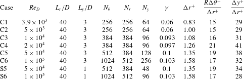
A summary of the LES runs performed is given in tables 1 and 2. We cover six different values of
 $Re_{D}$
in the sub-critical regime and three different values of
 $Re_{D}$
in the super-critical regime. For each case, we list the computational domain size defined by
 $L_{r}$
and
 $L_{y}$
and the mesh resolution in three directions,
 $N_{\unicode[STIX]{x1D703}}$
,
 $N_{r}$
and
 $N_{y}$
. We use a standard O-grid for all cases to ensure mesh orthogonality. The meshes are uniform in the circumferential and spanwise directions, while stretching is used in the wall-normal direction. The latter employs a tanh function, from which the wall-normal coordinate
 $r$
at index
 $k$
can be written as
 $$\begin{eqnarray}r(k)=R+L_{r}\frac{1-\tanh (\unicode[STIX]{x1D6FE}(L_{r}-\hat{r}(k)))}{\tanh (\unicode[STIX]{x1D6FE}L_{r})}.\end{eqnarray}$$
Here,
 $r=R$
defines the inner boundary and
 $r=L_{r}$
the outer boundary of the computational domain. The parameter
 $\hat{r}(k)$
is uniformly distributed from
 $r=R$
to
 $r=L_{r}$
, which means that
 $\hat{r}(k)=k(L_{r}-R)/N_{r}$
, while
 $\unicode[STIX]{x1D6FE}$
is the only stretching-control parameter and is also listed in both tables. The first five points above the cylinder surface were uniformly spaced to simplify implementation of the no-slip solid-wall boundary condition.
In most reported wall-resolved LES, the near-wall mesh resolution in the wall-parallel direction has not conformed to strict DNS standards. Generally, the cell spacing in wall-parallel directions is too coarse to accurately resolve the energy scales but is sufficient to provide a physical mean profile (Cabot & Moin Reference Cabot and Moin1999). The non-dimensional cell dimension based on the wall unit length
 $l^{+}\equiv \unicode[STIX]{x1D708}/u_{\unicode[STIX]{x1D70F}}$
can be extended up to approximately
 $130$
in the streamwise direction and to
 $30$
in the spanwise direction (Chapman Reference Chapman1979; Choi & Moin Reference Choi and Moin2012). For example, the turbulent channel-flow LES of Voelkl et al. (Reference Voelkl, Pullin and Chan2000) used cell sizes of
 $166\,l^{+}$
streamwise and
 $50\,l^{+}$
spanwise. For LES of flow over a cylinder, similar resolution has been utilized, such as in Lehmkuhl et al. (Reference Lehmkuhl, Rodríguez, Borrell, Chiva and Oliva2014), where 128 points represented the cylinder span.
Our relevant non-dimensional lengths are
 $\unicode[STIX]{x0394}r^{+}=\unicode[STIX]{x0394}r_{1}/l^{+}$
, with the subscript ‘1’ denoting the near-wall mesh, which is also the minimum in the domain,
 $\unicode[STIX]{x0394}y^{+}=\unicode[STIX]{x0394}y/l^{+}$
and
 $R\unicode[STIX]{x0394}\unicode[STIX]{x1D703}^{+}=R\unicode[STIX]{x0394}\unicode[STIX]{x1D703}/l^{+}$
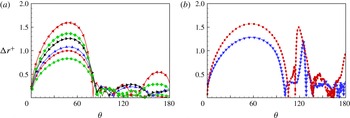
. These are shown in tables 1 and 2 for sub-critical and super-critical LES respectively. In figure 1(a), we plot
 $\unicode[STIX]{x0394}r^{+}$
versus
 $\unicode[STIX]{x1D703}$
for sub-critical flows, while 1(b) shows the same plot for super-critical LES. For all cases,
 $\unicode[STIX]{x0394}r^{+}$
is less than
 $1$
along most of the wall, except for regions around
 $\unicode[STIX]{x1D703}=50^{\circ }$
. This resolution is similar to other wall-resolved LES, for example Lehmkuhl et al. (Reference Lehmkuhl, Rodríguez, Borrell, Chiva and Oliva2014) and the periodic hill flow (Fröhlich et al.
Reference Fröhlich, Mellen, Rodi, Temmerman and Leschziner2005).
Plots of
 $\unicode[STIX]{x0394}r^{+}$
for (a) sub-critical cases and (b) super-critical cases.
 $Re_{D}$
value: (a) ●,
 $3900$
; ▪,
 $5000$
; ▴,
 $10^{4}$
; ▸,
 $2\times 10^{4}$
; ♦,
 $5\times 10^{4}$
; ◂,
 $10^{5}$
; (b) ▾,
 $3.5\times 10^{5}$
; ▪,
 $8.5\times 10^{5}$
.

3 The sub-critical regime
In the sub-critical region, the boundary-layer flow around the cylinder is laminar while transition to turbulence takes place in the free-shear layer. With increasing
 $Re_{D}$
, the transition region is found to gradually approach the cylinder surface near the separation region. In the experiment of Cantwell & Coles (Reference Cantwell and Coles1983), the flow with
 $Re_{D}=1.95\times 10^{5}$
already shows a clear transition behaviour near the cylinder surface. They chose
 $Re_{D}=1.4\times 10^{5}$
as a benchmark case to study the upper range of shear-layer transition. Similarly, we describe results with
 $Re_{D}$
from
 $3.9\times 10^{3}$
to
 $10^{5}$
. In this
 $Re_{D}$
range, Weidman (Reference Weidman1968) confirmed that the minimum pressure coefficient, Strouhal number and drag coefficient are approximately constant. The skin-friction measurement by Son & Hanratty (Reference Son and Hanratty1969) shows a uniform scaling using
 $Re_{D}^{1/2}$
in the attached part while exhibiting large variance in the separated region up to
 $Re_{D}=10^{5}$
. In this regime, we implement eight cases with the parameters listed in table 1.
3.1 Low Reynolds number:
 $Re_{D}=3.9\times 10^{3}$
to
$2\times 10^{4}$


3.1.1
$Re_{D}=3.9\times 10^{3}$

We begin with
 $Re=3.9\times 10^{3}$
, which is perhaps the most documented benchmark case in the literature. This will also serve as a validation case for the present wall-resolved LES code. Some experimental studies at this value of
 $Re_{D}$
focus on the character of the near-wall flow, including Norberg (Reference Norberg1993), who documents pressure-coefficient measurements, while others, for example Lourenco & Shih (Reference Lourenco and Shih1994), report results for mean velocity and turbulent intensity profiles in the near-wake region. In numerical simulation, Beaudan & Moin (Reference Beaudan and Moin1994) first emphasized this specific case. Subsequent work by Kravchenko & Moin (Reference Kravchenko and Moin2000) and You & Moin (Reference You and Moin2007) found a U-shaped mean velocity profile inside the recirculation bubble rather than a V-shape profile as measured in experiment by Lourenco & Shih (Reference Lourenco and Shih1994). Ma et al. (Reference Ma, Karamanos and Karniadakis2000) discussed this contradiction by performing simulation using different spanwise domains. Their mean velocity converges to a U-shape when using
 $L_{z}=\unicode[STIX]{x03C0}D$
, but to a V-shape for
 $L_{z}=2\unicode[STIX]{x03C0}D$
. Recently, Parnaudeau et al. (Reference Parnaudeau, Carlier, Heitz and Lamballais2008) performed both experiments and numerical simulation that supported the U-shaped mean velocity profile.
In comparison of the present LES results with available references, we choose the experimental data by Parnaudeau et al. (Reference Parnaudeau, Carlier, Heitz and Lamballais2008), the LES result by Beaudan & Moin (Reference Beaudan and Moin1994) and the DNS result (case II) in Ma et al. (Reference Ma, Karamanos and Karniadakis2000). Although the issue of V-shape versus U-shape of the mean streamwise velocity remains unresolved, we note that both the cited experiment and the simulations with
 $L_{z}=\unicode[STIX]{x03C0}D$
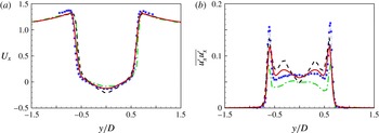
find a U-shaped profile. In figure 2(a), we plot the mean streamwise velocity along the
 $z$
direction at
 $x=1.06$
. We can conclude that the differences between different simulation results and experiment are small and at approximately the same level. The present LES agrees quite well with Kravchenko & Moin (Reference Kravchenko and Moin2000) except at around
 $y/D=0$
. Near the centreline
 $y/D=0$
, the present LES matches the valley value from experiments. In figure 2(b), we compare the streamwise turbulent intensity
 $\overline{u_{x}^{\prime }u_{x}^{\prime }}$
profiles of experiment and numerical simulations. All simulation results deviate substantially from the measurements in the region
 $y/d\in (-0.5,0.5)$
. The present LES agrees in the profile shape with the simulation result of Kravchenko & Moin (Reference Kravchenko and Moin2000).
Streamwise mean velocity profile (a) and turbulent intensity (b) at
 $x=1.06$
: ▪, experiments by Parnaudeau et al. (Reference Parnaudeau, Carlier, Heitz and Lamballais2008); ——, present LES; – – – –, LES by Kravchenko & Moin (Reference Kravchenko and Moin2000); — ⋅ —, DNS by Ma et al. (Reference Ma, Karamanos and Karniadakis2000).

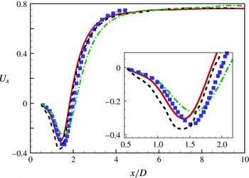
Streamwise mean velocity profile along the wake centreline,
 $Re_{D}=3900$
: ▪, experiments by Parnaudeau et al. (Reference Parnaudeau, Carlier, Heitz and Lamballais2008); ——, present LES; – – – –, LES by Kravchenko & Moin (Reference Kravchenko and Moin2000); — ⋅ —, LES by Parnaudeau et al. (Reference Parnaudeau, Carlier, Heitz and Lamballais2008).

We also compare the streamwise mean velocity in the wake centreline, as shown in figure 3. All simulation results can generally capture the behaviour of the
 $U_{x}$
distribution, which first decreases to a minimum value then recovers monotonically in the far-wake region. We note that in the region of decrease, the present LES agrees well with the experimental data, while in the recovery region, the present LES and the LES result by Kravchenko & Moin (Reference Kravchenko and Moin2000) are in reasonable agreement with each other and with the experiment by Parnaudeau et al. (Reference Parnaudeau, Carlier, Heitz and Lamballais2008).
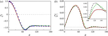
Variation of (a) the pressure coefficient
 $C_{p}(\unicode[STIX]{x1D703})$
and (b) the skin-friction coefficient
 $\overline{C_{f\unicode[STIX]{x1D703}}}(\unicode[STIX]{x1D703})$
along the cylinder surface: ——, present LES; ▫, experiments by Norberg (Reference Norberg1993); — ⋅ —, LES by Beaudan & Moin (Reference Beaudan and Moin1994); – – – –, DNS by Ma et al. (Reference Ma, Karamanos and Karniadakis2000).

The pressure coefficient
 $C_{p}$
is shown in figure 4(a). It can be seen that all data are in reasonable agreement with each other. The relative error of the present LES compared with experimental data is roughly 3 % at approximately
 $\unicode[STIX]{x1D703}=70^{\circ }$
and 5 % at
 $\unicode[STIX]{x1D703}=130^{\circ }$
. Furthermore, we show the skin-friction coefficient
 $\overline{C_{f\unicode[STIX]{x1D703}}}$
along the cylinder surface in figure 4(b), where the three skin-friction distributions agree reasonably with each other. In the inset of 4(b), we find that all three simulation results show a mean-flow secondary separation bubble, characterized by a region where
 $\overline{C}_{f\unicode[STIX]{x1D703}}$
becomes positive and then negative as
 $\unicode[STIX]{x1D703}$
increases. It can be seen that all results give a somewhat similar separation point and
 $\unicode[STIX]{x1D703}$
extent for this secondary bubble. Son & Hanratty (Reference Son and Hanratty1969) found that the separation angle for the secondary bubble decreases with increasing
 $Re_{D}$
. At
 $Re_{D}=5\times 10^{3}$
, their experimentally measured separation angle is approximately
 $120^{\circ }$
. Extrapolation of their results suggests a separation angle slightly larger than
 $120^{\circ }$
at
 $Re_{D}=3.9\times 10^{3}$
. In the present LES, the separation of the secondary bubble agrees well with this experiment, and takes place at an angle of
 $121^{\circ }$
, which is larger than the value of
 $110^{\circ }$
seen in other simulation results.
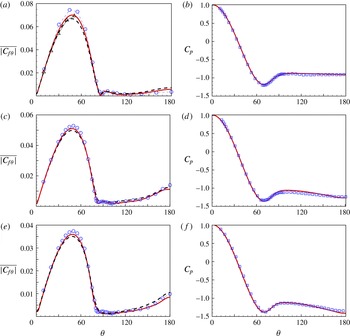
(a,c,e) Skin-friction coefficient
 $\overline{|C_{f\unicode[STIX]{x1D703}}|}$
and (b,d,f) pressure coefficient
 $C_{p}$
at different values of
 $Re_{D}$
. In (a,b),
 $Re_{D}=5\times 10^{3}$
; in (c,d),
 $Re_{D}=10^{4}$
; in (e,f),
 $Re_{D}=2\times 10^{4}$
. In (a,c,e): ——, solution of ODEs; – – – –, velocity-derivative method; ○, experiments by Son & Hanratty (Reference Son and Hanratty1969); ▵, theoretical estimate by Thom (Reference Thom1928). In (b,d,f): ——, LES; ▫, experiments by Weidman (Reference Weidman1968);

3.1.2
$Re_{D}=5\times 10^{3}\sim 2\times 10^{4}$

Next, we discuss LES at
 $Re_{D}=5\times 10^{3}$
,
 $10^{4}$
and
 $2\times 10^{4}$
, with emphasis on comparison of
 $\overline{|C_{f\unicode[STIX]{x1D703}}|}$
LES results with experiments by Son & Hanratty (Reference Son and Hanratty1969). Their experiment employed the technique of mass transfer measurement, in which the velocity gradient at the surface is related to the averaged mass transfer rate of a test chemical species. In the experiment, the mass transfer rate in the wall-parallel plane is derived from the rate of reaction and thus can be directly computed from the measured electrical current output. This enables measurement of the time-averaged absolute value of the velocity gradient at the wall, which corresponds to
 $\overline{|C_{f\unicode[STIX]{x1D703}}|}$
in the present LES.
Comparison of LES results for
 $\overline{|C_{f\unicode[STIX]{x1D703}}|}$
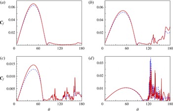
with these data is shown in figure 5. Large-eddy simulation results using both the direct velocity-derivative method and the ODE method are shown. Both methods show good agreement with the data except near the region of
 $\unicode[STIX]{x1D703}=50^{\circ }$
. Near the peak value, the ODE
 $\overline{|C_{f\unicode[STIX]{x1D703}}|}$
is generally larger than values using the velocity derivative, while still approximately 3 % lower than the experimental data. Additionally, we can also estimate
 $\overline{|C_{f\unicode[STIX]{x1D703}}|}$
on the front part of the cylinder by theoretically coupling the pressure distribution to
 $\overline{|C_{f\unicode[STIX]{x1D703}}|}$
using the method of Thom (Reference Thom1928). A pressure distribution is needed, and here it is obtained from the experiment of Weidman (Reference Weidman1968). The peak of this theoretical estimate generally agrees with the result from the ODE method, which provides a form of validation of this approach. For the other two cases,
 $Re_{D}=10^{4}$
and
 $2\times 10^{4}$
, both LES results are in reasonable agreement with experiments.
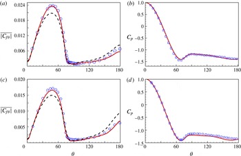
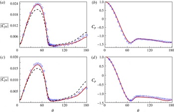
(a,c) Skin-friction coefficient
 $\overline{|C_{f\unicode[STIX]{x1D703}}|}$
and (b,d) pressure coefficient
 $C_{p}$
at different values of
 $Re_{D}$
. In (a,b),
 $Re_{D}=5\times 10^{4}$
; in (c,d),
 $Re_{D}=10^{5}$
. In (a,c): ——, solution of ODEs; – – – –, velocity-derivative method; ○, experiments by Son & Hanratty (Reference Son and Hanratty1969). In (b,d): ——, LES; ▫, experiments by Weidman (Reference Weidman1968).
3.2
$Re_{D}=5\times 10^{4}$
and
$10^{5}$


At these higher values of
 $Re_{D}$
, the boundary layer becomes sufficiently thin so as to require a fine near-wall mesh. Two coefficients,
 $\overline{|C_{f\unicode[STIX]{x1D703}}|}$
and
 $C_{p}$
, are shown in figure 6. It is notable that, for these two cases, the value of
 $\overline{|C_{f\unicode[STIX]{x1D703}}|}$
estimated using the ODE method shows better comparison with experiments than the velocity-derivative method, especially in the region around
 $\unicode[STIX]{x1D703}=50^{\circ }$
.
3.2.1
$\overline{|C_{f\unicode[STIX]{x1D703}}|}$
at
$Re_{D}=10^{5}$


We further compare the skin friction with other experiments with emphasis on the peak region; see figure 7(a). Here, we cite four experimental data sets and one theoretical estimate based on the experimental data. These four experiments used different methods for skin-friction measurement. Both Giedt (Reference Giedt1951) and Achenbach (Reference Achenbach1968) calibrated the skin friction from the measured pressure distribution. Son & Hanratty (Reference Son and Hanratty1969) employed a mass transfer analogue, where the velocity gradient is derived from measurement of a mass transfer coefficient, while Fage & Falkner (Reference Fage and Falkner1931) directly measured the velocity component around the cylinder using a Pitot tube. Thus, in the first three experiments, the skin-friction coefficients were measured by using some form of momentum conservation, not unlike our ODE method, while Fage & Falkner (Reference Fage and Falkner1931) instead used the velocity components directly. Fage & Falkner (Reference Fage and Falkner1931) claimed that the use of velocity directly to measure the velocity gradient gives non-negligible errors. Following careful examination of results at this specific value of
 $Re_{D}$
with the theoretical method of Thom (Reference Thom1928), they estimated it to be in error by a factor of approximately
 $1.16$
. This theoretical estimate is one that we refer to presently.
We observe that the three experimental measurements inferred from momentum conservation and the theoretical estimate by Fage & Falkner (Reference Fage and Falkner1931) agree well near the peak region, although results vary between experiments from the 1920s and the 1960s. These results also match our LES results using the passive ODE method quite well. The experiment by Fage & Falkner (Reference Fage and Falkner1931), which provided the only experimental data obtained by direct measurement of velocity components, is quite close to the result in the present LES using the velocity-derivative method. Our tentative conclusion is that, while for the present LES, values of
 $\overline{|C_{f\unicode[STIX]{x1D703}}|}$
calculated using the direct velocity-gradient and ODE methods differ from each other, they both reasonably match the experimental data from corresponding experiments.
Comparison of
 $\overline{|C_{f\unicode[STIX]{x1D703}}|}$
at
 $Re_{D}=10^{5}$
. Experiments: ▫, by Achenbach (Reference Achenbach1968); ○, by Son & Hanratty (Reference Son and Hanratty1969); ♢, by Giedt (Reference Giedt1951); ▵, modification from Fage & Falkner (Reference Fage and Falkner1931); ▿, by Fage & Falkner (Reference Fage and Falkner1931), direct derivation of velocity. Large-eddy simulations: ——, using ODE; – – – –, using velocity components; — ⋅ —, using mean ODE, (b).

The above suggests a question concerning the source of discrepancy between the two classes of skin-friction coefficient measurements/LES results. To explain this, we revisit our two methods used. In (2.12), the velocity derivative is a linear function of the velocity components, which implies that any strong fluctuations in the instantaneous flow velocity will finally be cancelled out in favour of the averaged value. In contrast, in using the ODE approach, the nonlinear convective term in (2.17) gives a strong instantaneous contribution. To examine this, we introduce another way to measure the skin-friction coefficient, which is a steady version of the ODE, referred to as the mean-ODE method. In this version, the unsteady term is not present, and so a simple formula can be obtained as
 $\unicode[STIX]{x1D702}_{0}=h\widetilde{F_{\unicode[STIX]{x1D703}}}/\unicode[STIX]{x1D708}$
. This result is plotted in figure 7(b), together with results using the other two methods. Interestingly, the mean-ODE results generally are similar to the direct velocity-derivative method, and both are somewhat different from the results using the full ODE. This comparison provides evidence that the difference between the velocity-derivative and ODE methods is due to contributions of the averaged instantaneous fluctuations of the velocity. We note in passing that these differences are a result of insufficient resolution at the wall. For an extremely fine mesh at the wall, finer than is presently practicable, we would expect all three methods to agree.
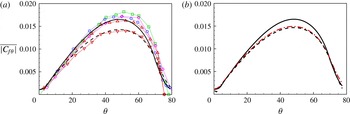
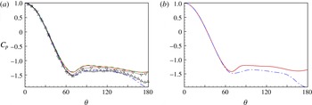
Comparison of the pressure coefficient
 $C_{p}$
using different spanwise domains. In (a),
 $Re_{D}=5\times 10^{4}$
. Experiments by Szepessy & Bearman (Reference Szepessy and Bearman1992) at
 $Re_{D}=4\times 10^{4}$
: ▵,
 $L_{y}/D=1$
; ▿,
 $L_{y}/D=6.7$
. Present LES at
 $Re_{D}=5\times 10^{4}$
: – – – –,
 $L_{y}/D=6$
; ——,
 $L_{y}/D=3$
; — ⋅ —,
 $L_{y}/D=1$
. In (b),
 $Re_{D}=10^{5}$
: ——,
 $L_{y}/D=3$
; — ⋅ —,
 $L_{y}/D=1$
.

3.2.2 Effect of the spanwise domain
In the previous cases, all LES employ the same spanwise domain
 $L_{y}/D=3$
. This parameter, when used for
 $Re_{D}=3.9\times 10^{3}$
, has been found to be sufficient for many previous simulations. With increasing
 $Re_{D}$
, it is generally believed that the required spanwise domain will decrease because the largest flow structure in the spanwise direction should decrease with shrinking boundary-layer thickness. There is, however, no real consensus on a necessary domain size at a given
 $Re_{D}$
. Some simulations with
 $Re_{D}$
values of approximately
 $10^{5}$
, for example by Breuer (Reference Breuer2000), prefer
 $L_{y}/D=1$
. Experiments by Szepessy & Bearman (Reference Szepessy and Bearman1992) show that for
 $Re_{D}=4\times 10^{4}$
,
 $L_{y}/D=1$
gives quite different results from
 $L_{y}/D=10$
, even for the
 $C_{p}$
distribution. Although results with
 $L_{y}/D=1$
used in experiment cannot perhaps be directly related to LES using a different domain extent, it is still interesting to compare these experiments with the present LES at
 $Re_{D}=5\times 10^{4}$
; see figure 8(a). Our LES with
 $L_{y}/D=6$
and
 $L_{y}/D=3$
gives reasonably close results to the experimental data at
 $L_{y}/D=6.7$
in the attached-flow region. The case with
 $L_{y}/D=1$
shows a sharp drop after flow separation, which is qualitatively similar to the experiments. We also show results for
 $Re_{D}=10^{5}$
with
 $L_{y}/D=3$
and
 $L_{y}/D=1$
in figure 8(b), where similar performance is found. This indicates that for the present LES,
 $L_{y}/D=1$
is still not sufficient in this
 $Re_{D}$
range. This suggests that, with increasing
 $Re_{D}$
in the sub-critical regime, accurate LES requires a wide spanwise domain such as
 $L_{y}/D=3$
. It is only when turbulence inside the shear layer reaches the cylinder surface that the spanwise domain requirement will decrease substantially due to the presence of smaller turbulent structures attached within the separated region.
3.3 Notes on the sub-critical regime
3.3.1 Skin-friction coefficients:
$\overline{C_{f}}$
and
$\overline{|C_{f\unicode[STIX]{x1D703}}|}$


It is of interest to compare different skin-friction coefficients. Here, we focus on
 $\overline{C_{f}}$
and
 $\overline{|C_{f\unicode[STIX]{x1D703}}|}$
. These are always positive, with
 $\overline{C_{f}}$
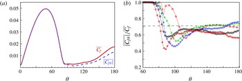
including the contribution from spanwise fluctuations. In figure 9(a), we compare the two coefficients at
 $Re_{D}=10^{4}$
. From the forward stagnation point until
 $\unicode[STIX]{x1D703}\approx 80^{\circ }$
, the two coefficients are almost the same, indicating that the near-wall spanwise velocity component and its wall-normal derivative are negligible in this region. For
 $\unicode[STIX]{x1D703}>80^{\circ }$
,
 $\overline{C_{f}}$
is always larger than
 $\overline{|C_{f\unicode[STIX]{x1D703}}|}$
owing to non-negligible
 $C_{fy}$
in this region. Figure 9(b) shows the ratio
 $\overline{|C_{f\unicode[STIX]{x1D703}}|}/\overline{C_{f}}$
for LES at five different values of
 $Re_{D}$
. For
 $Re_{D}=10^{4},\,2\times 10^{4}$
, it can be observed that the ratio tends to approximately
 $1/\sqrt{2}$
for
 $\unicode[STIX]{x1D703}>120$
, which implies that the magnitude of
 $C_{fy}$
is similar to that of
 $C_{f\unicode[STIX]{x1D703}}$
. For
 $Re_{D}=5\times 10^{4}$
and
 $10^{5}$
, the ratio decreases below
 $1/\sqrt{2}$
, showing the importance of spanwise velocity gradients in the large-scale separated region.
(a) Comparison of
 $\overline{|C_{f\unicode[STIX]{x1D703}}|}$
and
 $\overline{C_{f}}$
at
 $Re_{D}=10^{4}$
. (b) Ratio of
 $\overline{|C_{f\unicode[STIX]{x1D703}}|}$
to
 $\overline{C_{f}}$
, for the following values of
 $Re_{D}$
: ▫,
 $5\times 10^{3}$
; ▵,
 $10^{4}$
; ▿,
 $2\times 10^{4}$
; ♢,
 $5\times 10^{4}$
; ◃,
 $10^{5}$
.

3.3.2 Comparison with flat-plate boundary-layer flow
If we consider the stagnation point as the leading edge of a flat plate (FP), the boundary-layer flow around the cylinder away from the stagnation point can be compared with the FP boundary-layer flow based on a definition of length scale that is an analogue of
 $Re_{x}=U_{\infty }/x\unicode[STIX]{x1D708}$
, with
 $x$
measured from the leading edge in the FP case. Here, we define a Reynolds number
 $Re_{s}=U_{\infty }\,s/\unicode[STIX]{x1D708}$
based on the arclength
 $s$
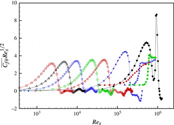
from the forward stagnation point. We also cite three DNS results for FP turbulent boundary-layer flow. One is from Wu & Moin (Reference Wu and Moin2009), where a turbulent perturbation is introduced at the inflow, while the other two are H-type and K-type transition (Sayadi, Hamman & Moin Reference Sayadi, Hamman and Moin2013), where a perturbation is generated by providing a blowing and suction boundary condition for the wall-normal velocity along a spanwise strip. In figure 10, we plot
 $\overline{C_{f\unicode[STIX]{x1D703}}}\,Re_{s}^{1/2}$
versus
 $Re_{s}$
for different cases, including five
 $Re_{D}$
values from the present LES and another two results from experimental data by Achenbach (Reference Achenbach1968). Three DNS of FP boundary-layer transition are also shown. It can be seen that only the cylinder flow at
 $Re_{D}=8.5\times 10^{5}$
lies beyond the region of equivalent FP boundary-layer transition, while all other cases, including
 $Re_{D}=2.6\times 10^{5}$
, are not within the region of equivalent FP boundary-layer transition. It should be emphasized that the case
 $Re_{D}=2.6\times 10^{5}$
has some overlap with DNS by Wu & Moin (Reference Wu and Moin2009). Because the FP and cylinder flows are rather different in both geometry and surface pressure-gradient distribution, the present comparison is not strictly appropriate quantitatively. We argue that it does, however, indicate the potential importance of the presence of a boundary-layer perturbation on boundary-layer transition in cylinder flow at a given
 $Re_{D}$
.
4 The super-critical regime
Since the beginning of the last century, there have been many experiments at values of
 $Re_{D}$
within and beyond the drag-crisis (or so-called critical) regime. While different experimental measurements of the same quantity that depend on
 $Re_{D}$
do not always agree, the cumulative trend of measurements has clarified many factors that might influence the flow, including the aspect ratio, turbulent intensity in the inflow, compressibility effects and surface roughness. Schewe (Reference Schewe1986) concluded that in the super-critical regime, the flow is very sensitive to even a small perturbation, which may be natural or artificial.
In terms of numerical simulation, we note that a weak numerical-type instability might be sufficient to alias as a natural perturbation for some forms of flow transitions. However, numerical perturbation can often be decreased in intensity by using finer and more regular meshes. For a case where some form of numerical perturbation is not sufficient to result in a natural transition, an artificial perturbation may be required.
With this in mind, we performed a series of LES in the super-critical regime, as shown in table 2. Two cases with a relatively coarse mesh at
 $Re_{D}=2.6\times 10^{5}$
and
 $Re_{D}=8.5\times 10^{5}$
were first implemented. These two are presented as LES with no externally applied flow disturbance but with possible grid or small-scale inherent numerical perturbation resulting from, for example, fluctuating discretization error. Two other LES with finer meshes were performed for
 $Re_{D}=3.5\times 10^{5}$
and
 $8.5\times 10^{5}$
. In these two cases, the expected numerical perturbation was found to be so small that an artificial perturbation was required to trip the transition. The artificial perturbation used was a blowing–suction-type boundary condition, described in detail in appendix A. In the following discussion of these and other LES, unless specified otherwise, the ODE method is used to calculate skin friction due to its better agreement with experimental data for low-
 $Re_{D}$
cases.
Plot of
 $\overline{C_{f\unicode[STIX]{x1D703}}}Re_{s}^{1/2}$
versus
 $Re_{s}$
, where
 $Re_{s}=s\,U_{\infty }/\unicode[STIX]{x1D708}$
: comparison between flow over cylinder and flat-plate boundary-layer flow. Present LES: ▫,
 $5\times 10^{3}$
; ▵,
 $10^{4}$
; ▿,
 $2\times 10^{4}$
; ♢,
 $5\times 10^{4}$
; ◃,
 $10^{5}$
. Experiment by Achenbach (Reference Achenbach1968): ▾,
 $3.5\times 10^{5}$
; ♦,
 $8.5\times 10^{5}$
. Direct numerical simulation of zero-pressure-gradient turbulent boundary layer (ZPGTBL): ▪, by Wu & Moin (Reference Wu and Moin2009); ▴, K-transition by Sayadi et al. (Reference Sayadi, Hamman and Moin2013); ●, H-transition by Sayadi et al. (Reference Sayadi, Hamman and Moin2013).

Plots of (a)
 $\overline{C_{f\unicode[STIX]{x1D703}}}$
and (b)
 $C_{p}$
for
 $Re_{D}=2.6\times 10^{5}$
: ▫, experiments by Achenbach (Reference Achenbach1968); ○, experiments by Fage & Falkner (Reference Fage and Falkner1931); ▵, experiments by Giedt (Reference Giedt1951); ——, present LES.

Plots at
 $Re_{D}=3.5\times 10^{5}$
. (a) Plots of
 $\overline{C_{f\unicode[STIX]{x1D703}}}$
(– – – –) and
 $\overline{|C_{f\unicode[STIX]{x1D703}}|}$
(——). (b) Plots of
 $C_{p}$
: ○, experiments by Bursnall & Loftin (Reference Bursnall and Loftin1951); ▫, LES by Lehmkuhl et al. (Reference Lehmkuhl, Rodríguez, Borrell, Chiva and Oliva2014); ——, present LES.

Plots at
 $Re_{D}=3.5\times 10^{5}$
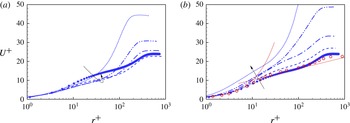
. Evolution of the scaled mean streamwise velocity
 $U^{+}$
along the cylinder surface in the range of
 $127.5^{\circ }\leqslant \unicode[STIX]{x1D703}\leqslant 144^{\circ }$
. In (a):
 $\cdots \cdots$
,
 $127.5^{\circ }$
; — ⋅ ⋅ —,
 $128^{\circ }$
; — ⋅ —,
 $128.5^{\circ }$
; – – – –,
 $129.5^{\circ }$
; ♦,
 $132.5^{\circ }$
. In (b): ♦,
 $132.5^{\circ }$
; – – – –,
 $134^{\circ }$
; — ⋅ —,
 $136^{\circ }$
; — ⋅ ⋅ —,
 $140.5^{\circ }$
,
 $\cdots \cdots$
,
 $143.5^{\circ }$
; ○, ZPGTBL DNS by Sayadi et al. (Reference Sayadi, Hamman and Moin2013). Log line:
 $U^{+}=\log (r^{+})/0.384+4.127$
.

4.1
$Re_{D}=2.6\times 10^{5}$
and
$3.5\times 10^{5}$


We first discuss
 $Re_{D}=2.6\times 10^{5}$
, for which results are shown in figure 11. For this low-resolution case, both skin-friction pressure coefficients obtained from the LES agree reasonably with experimental data by Achenbach (Reference Achenbach1968).
Next, we consider
 $Re_{D}=3.5\times 10^{5}$
with fine resolution. In this case, without artificial perturbation, the flow remains in a sub-critical state. Once the perturbation is applied, the boundary-layer flow quickly undergoes transition to turbulence accompanied by a sharp decrease of the drag coefficient. The skin-friction and pressure coefficients are shown in figure 12. Here,
 $C_{p}$
is found to agree reasonably with existing experiments. The coefficient
 $\overline{C_{f\unicode[STIX]{x1D703}}}$
becomes negative at approximately
 $\unicode[STIX]{x1D703}=106^{\circ }$
, which implies a separation. This separation bubble is found to reattach downstream at approximately
 $\unicode[STIX]{x1D703}=127^{\circ }$
followed by a spike of
 $\overline{C_{f\unicode[STIX]{x1D703}}}$
. This indicates that the transition takes place within the shear layer atop the small separation bubble. After the flow, now in a turbulent state, reattaches, it develops further until separation again occurs at approximately
 $\unicode[STIX]{x1D703}=150^{\circ }$
. This separation then forms the large-scale separation region downstream of the cylinder.
To show the flow transition into turbulence, we choose several slices in the range
 $127^{\circ }<\unicode[STIX]{x1D703}<150^{\circ }$
to examine the streamwise velocity profile
 $U^{+}(r^{+})$
. Figure 13 plots seven velocity profiles with the local wall-normal coordinate scaled using the viscous unit
 $\unicode[STIX]{x1D708}/u_{\unicode[STIX]{x1D70F}}$
and
 $U^{+}=U/u_{\unicode[STIX]{x1D70F}}$
, where
 $U$
is the local mean velocity component tangential to the cylinder surface. In figure 13(a), the transition into turbulence can be observed by first the decrease of
 $U^{+}$
and then the formation of a log-like zone. A turbulent velocity profile can be found at
 $\unicode[STIX]{x1D703}=132.5^{\circ }$
, which agrees well with the DNS of the ZPGTBL case by Sayadi et al. (Reference Sayadi, Hamman and Moin2013), as shown in figure 13(b). Also in figure 13(b), we plot several velocity profiles at other downstream locations. Since the flow is further developed due to the effect of the adverse pressure gradient, it can be seen that the velocity profile is gradually lifted towards a form typical of an adverse-pressure-gradient flow with a large wake factor; see, for example, Monty, Harun & Marusic (Reference Monty, Harun and Marusic2011). At
 $\unicode[STIX]{x1D703}=143.5^{\circ }$
, the flow does not show a turbulent-boundary-layer-like velocity profile, and further downstream, turbulent flow separation takes place. In figure 14, we show similar plots, with
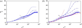
 $U^{+}$
scaled using the skin-friction coefficient from the velocity-derivative method. It can be found that scaling using the two methods gives no substantial difference in this turbulent flow region.
Plots at
 $Re_{D}=3.5\times 10^{5}$
. Here,
 $U^{+}$
is scaled using the skin-friction coefficient from the velocity-derivative method. The same symbols as in figure 13 are used.

Plots of (a)
 $\overline{C_{f\unicode[STIX]{x1D703}}}$
and (b)
 $C_{p}$
for
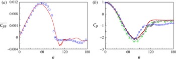
 $Re_{D}=8.5\times 10^{5}$
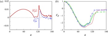
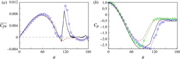
: ▫, experiments by Achenbach (Reference Achenbach1968); ▵, experiments by Shih et al. (Reference Shih, Wang, Coles and Roshko1993); – – – –, coarse-mesh LES; ——, fine-mesh LES.

4.2
$Re_{D}=8.5\times 10^{5}$

We extend the LES to
 $Re_{D}=8.5\times 10^{5}$
to compare the present LES with experiments by Achenbach (Reference Achenbach1968). In figure 15, we plot
 $\overline{C_{f\unicode[STIX]{x1D703}}}$
and
 $C_{p}$
for results from both the coarse-mesh and fine-mesh cases. It is interesting that for the low-resolution LES in figure 15, although
 $\overline{C_{f\unicode[STIX]{x1D703}}}$
shows the correct behaviour over the windward part of the cylinder, it does not show the spike seen in the experimental data of Achenbach (Reference Achenbach1968). Further, neither does the
 $C_{p}$
surface distribution follow the data of Achenbach (Reference Achenbach1968), but instead agrees better with the measurements of Shih et al. (Reference Shih, Wang, Coles and Roshko1993). This can perhaps be interpreted as that the numerical perturbation introduced on the coarse mesh is not equivalent to a physical disturbance, and is difficult to quantify.
For the fine-resolution case, we are able to reproduce the boundary-layer transition. The plot of
 $\overline{C_{f\unicode[STIX]{x1D703}}}$
in figure 15 shows that the present LES accurately captures the spike in the experimental data by Achenbach (Reference Achenbach1968). The difference between the fine-resolution case and Achenbach’s experiment is the existence of a mean-flow separation bubble. As shown in figure 15(a), the LES shows negative values of
 $\overline{C_{f\unicode[STIX]{x1D703}}}$
in the range
 $105^{\circ }<\unicode[STIX]{x1D703}<115^{\circ }$
, which implies the existence of a small separation bubble. This is not seen in experimental data. The explanation for this discrepancy is perhaps that
 $Re_{D}=8.5\times 10^{5}$
is near the upper edge of the super-critical regime, which means that the small prior separation bubble, if it exists, should be very thin. This difference from experiment might then be ascribed to the difficulty of experimental measurement in capturing the small prior separation bubble. The separation bubble is discussed in more detail in § 6.
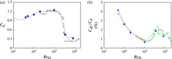
4.3 Drag coefficient
From the distribution of
 $C_{p}(\unicode[STIX]{x1D703})$
and
 $\overline{C_{f\unicode[STIX]{x1D703}}}(\unicode[STIX]{x1D703})$
, the total drag coefficient
 $C_{d}$
for the cylinder can be obtained. This is plotted in figure 16(a). Figure 16(b) plots the percentage of friction drag coefficient
 $C_{df}$
to the total drag coefficient
 $C_{d}$
as a function of
 $Re_{D}$
. It can be seen that the present LES generally agrees with the experiments of Son & Hanratty (Reference Son and Hanratty1969) and Achenbach (Reference Achenbach1968). For low
 $Re_{D}$
, the skin-friction contribution can be up to 4 %, while for higher
 $Re_{D}$
within the sub-critical range, skin friction accounts for approximately 1 % of the total drag. Interestingly, this doubles during the drag crisis and then rapidly declines at larger
 $Re_{D}$
. We emphasize again that although the contribution of
 $\overline{C_{f\unicode[STIX]{x1D703}}}$
to
 $C_{d}$
is small, the skin-friction behaviour remains quite important since it is the principal indication of near-wall dynamics including flow separation.
(a) Drag coefficient
 $C_{d}$
and (b) the percentage of friction drag coefficient
 $C_{df}$
to total drag coefficient
 $C_{d}$
: ●, present LES; ▵, experiment by Schewe (Reference Schewe1983); ▫, experiment by Son & Hanratty (Reference Son and Hanratty1969); ▿, experiment by Achenbach (Reference Achenbach1968).

5 Boundary-layer development
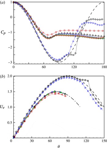
In the study of Achenbach (Reference Achenbach1968), the pressure distribution on the cylinder surface in the super-critical regime is close to that for potential flow but very different from potential flow in the sub-critical regime. The
 $C_{p}(\unicode[STIX]{x1D703})$
variations in the present LES are collected here in figure 17(a) to illustrate this difference. We can see that
 $C_{p}$
generally shows two different types; the first up to and including
 $Re_{D}=10^{5}$
has a small minimal value followed by a plateau, while the second for
 $Re_{D}>10^{5}$
is reasonably close to the potential result
 $C_{p}=2\cos 2\unicode[STIX]{x1D703}-1$
up to
 $\unicode[STIX]{x1D703}=150^{\circ }$
.
This difference suggests a classification of boundary-layer behaviour. Since there is not an outer uniform flow, the definition of the boundary layer requires some care. A reasonable metric is to use the radial location of the first maximum value of
 $u_{\unicode[STIX]{x1D703}}$
along the radial direction from the wall as the outer edge of the boundary layer. This maximum velocity is denoted as
 $U_{e}$
. In figure 18, we plot the mean
 $U_{e}$
along the
 $\unicode[STIX]{x1D703}$
direction for both the sub-critical and super-critical cases. The super-critical cases collapse onto the potential result
 $U_{e}=2\sin \unicode[STIX]{x1D703}$
, while all of the sub-critical cases also generally collapse onto one curve obtained empirically as
 $U_{e}=1.5\sin (1.25\unicode[STIX]{x1D703})$
, which is significantly different from the potential flow result. We note that for the sub-critical cases, the near-surface flow does not exhibit an identifiable near-wall first maximum value of
 $u_{\unicode[STIX]{x1D703}}$
in the separation region, and so
 $U_{e}$
is plotted only up to approximately
 $\unicode[STIX]{x1D703}=90^{\circ }$
.
(a) Pressure distribution
 $C_{p}$
; – – – –, potential flow
 $C_{p}=2\cos 2\unicode[STIX]{x1D703}-1$
. (b) External velocity
 $U_{e}$
; – – – –, potential flow
 $U_{e}=2\sin \unicode[STIX]{x1D703}$
; — ⋅ —,
 $U_{e}=1.5\sin (1.25\unicode[STIX]{x1D703})$
. Value of
 $Re_{D}$
: ▫,
 $5000$
; ▵,
 $10^{4}$
; ▿,
 $2\times 10^{4}$
; ♢,
 $5\times 10^{4}$
; ◃,
 $10^{5}$
; ○,
 $3.5\times 10^{5}$
; ▹,
 $8.5\times 10^{5}$
.

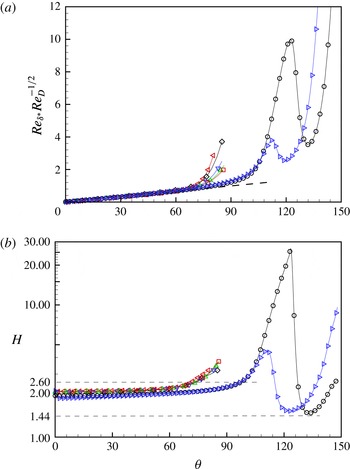
(a) Distribution of
 $Re_{\unicode[STIX]{x1D6FF}^{\ast }}Re_{D}^{-1/2}$
and (b) shape factor
 $H$
along the cylinder surface. In (a): – – – –,
 $Re_{\unicode[STIX]{x1D6FF}^{\ast }}Re_{D}^{-1/2}=0.011\unicode[STIX]{x1D703}$
. Value of
 $Re_{D}$
: ▫,
 $5000$
; ▵,
 $10^{4}$
; ▿,
 $2\times 10^{4}$
; ♢,
 $5\times 10^{4}$
; ◃,
 $10^{5}$
; ○,
 $3.5\times 10^{5}$
; ▹,
 $8.5\times 10^{5}$
.

With increasing
 $Re_{D}$
, the boundary-layer thickness at a given
 $\unicode[STIX]{x1D703}$
will reduce gradually and the maximum
 $u_{\unicode[STIX]{x1D703}}$
boundary-layer thickness remains a good measure. Using
 $U_{e}(\unicode[STIX]{x1D703})$
as an outer reference speed, we can calculate Reynolds numbers based on different measures of boundary-layer thickness. These are
 $$\begin{eqnarray}Re_{\unicode[STIX]{x1D6FF}^{\ast }}\equiv \frac{U_{e}\unicode[STIX]{x1D6FF}^{\ast }}{\unicode[STIX]{x1D708}}=\frac{u_{\unicode[STIX]{x1D70F}}\unicode[STIX]{x1D6E5}}{\unicode[STIX]{x1D708}}\equiv Re_{\unicode[STIX]{x1D70F}},\end{eqnarray}$$
with
 $\unicode[STIX]{x1D6FF}^{\ast }$
the local boundary-layer displacement thickness,
 $\unicode[STIX]{x1D6E5}\equiv \unicode[STIX]{x1D6FF}^{\ast }U_{e}/u_{\unicode[STIX]{x1D70F}}$
the Rotta–Clauser length scale and
 $Re_{\unicode[STIX]{x1D70F}}$
the Kármán number based on
 $\unicode[STIX]{x1D6E5}$
. It is expected that
 $Re_{\unicode[STIX]{x1D6FF}^{\ast }}$
at a given
 $\unicode[STIX]{x1D703}$
in the attached-flow region will increase with increasing
 $Re_{D}$
. In figure 18(a), we show the scaled quantity
 $Re_{\unicode[STIX]{x1D6FF}^{\ast }}Re_{D}^{-1/2}$
, which reasonably collapses onto the empirical fit
 $Re_{\unicode[STIX]{x1D6FF}^{\ast }}Re_{D}^{-1/2}\approx 0.011\,\unicode[STIX]{x1D703}$
up to
 $\unicode[STIX]{x1D703}=\unicode[STIX]{x1D703}_{c}$
. For the sub-critical cases,
 $\unicode[STIX]{x1D703}_{c}$
can be up to
 $60^{\circ }$
, while up to
 $80^{\circ }$
for the super-critical cases. Above this
 $\unicode[STIX]{x1D703}_{c}$
,
 $Re_{\unicode[STIX]{x1D6FF}^{\ast }}Re_{D}^{-1/2}$
shows an increasing tendency for all
 $Re_{D}$
. The two super-critical cases show an increase and subsequent decrease, due to the existence of a small separation bubble, and finally an increase again following transition and the reattached boundary layer.
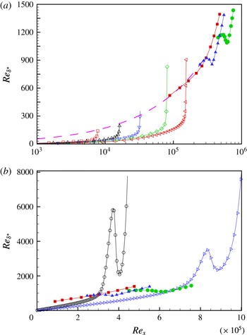
Plots of
 $Re_{\unicode[STIX]{x1D6FF}^{\ast }}$
versus
 $Re_{s}=s\,U_{\infty }/\unicode[STIX]{x1D708}$
for (a) sub-critical cases and (b) super-critical cases; – – – –, Blasius flow. Present LES,
 $Re_{D}$
value: ▫,
 $5000$
; ▵,
 $10^{4}$
; ▿,
 $2\times 10^{4}$
; ♢,
 $5\times 10^{4}$
; ◃,
 $10^{5}$
; ○,
 $3.5\times 10^{5}$
; ▹,
 $8.5\times 10^{5}$
. Direct numerical simulation of ZPGTBL: ▪, by Wu & Moin (Reference Wu and Moin2009); ▴, K-transition by Sayadi et al. (Reference Sayadi, Hamman and Moin2013); ●, H-transition by Sayadi et al. (Reference Sayadi, Hamman and Moin2013).

The shape factor
 $H$
, which is the ratio of the displacement boundary-layer thickness to the momentum boundary-layer thickness, is plotted in figure 18(b). It is seen that
 $H$
shows a modest increasing tendency extending from the stagnation point to
 $\unicode[STIX]{x1D703}_{c}$
. For the super-critical cases,
 $H$
rapidly increases above
 $\unicode[STIX]{x1D703}=\unicode[STIX]{x1D703}_{c}$
, reaches a value of
 $O(10)$
and decreases sharply to a valley value. This development of
 $H$
is quite similar to that seen in the FP boundary-layer transition with a laminar separation bubble, as shown by Simens (Reference Simens2008) in his figure 5.8(b). It should be emphasized that, in the transition of FP boundary-layer flow,
 $H$
in the turbulent part shows a slowly decreasing tendency around 1.44 within a finite development distance, as the flow is nominally zero pressure gradient. This kind of
 $H$
behaviour can be found in Simens (Reference Simens2008) and Sayadi et al. (Reference Sayadi, Hamman and Moin2013). It can be seen that the valley values of the present super-critical cases almost touch this value, which could provide evidence of the similarity between the present turbulent boundary-layer flow and the FP turbulent boundary-layer flow. The later development of
 $H$
above the location of the valley value is a response to the adverse-pressure-gradient effect and will not be further discussed. In figure 19(a,b), we show
 $Re_{\unicode[STIX]{x1D6FF}^{\ast }}$
versus
 $Re_{s}$
for sub-critical cases and super-critical cases respectively together with three DNS results for the FP turbulent boundary-layer flow. It can be seen that, for the sub-critical cases,
 $Re_{\unicode[STIX]{x1D6FF}^{\ast }}$
does not reach sufficiently high values to indicate transition prior to the onset of laminar separation. For
 $Re=3.5\times 10^{5}$
, the values of
 $Re_{s}$
reached lie within the
 $Re_{x}$
region where transition takes place in the FP boundary-layer flow.
Skin-friction coefficient
 $\overline{C_{f\unicode[STIX]{x1D703}}}$
for increasing sub-critical
 $Re_{D}$
: ▫,
 $5000$
; ▵,
 $10^{4}$
; ▿,
 $2\times 10^{4}$
; ♢,
 $5\times 10^{4}$
; ◃,
 $10^{5}$
.

6 Separation
6.1 The sub-critical regime
The skin-friction behaviour reveals the detailed properties of separation. Generally, in two-dimensional flow, it is considered that the zero crossing of
 $\overline{C_{f\unicode[STIX]{x1D703}}}$
represents the location of separation or reattachment. Presently, this can refer only to the nominally two-dimensional mean flow. In figure 20, we plot
 $\overline{C_{f\unicode[STIX]{x1D703}}}$
for all present LES in the sub-critical regime. In all LES with different values of
 $Re_{D}$
,
 $\overline{C_{f\unicode[STIX]{x1D703}}}$
is of almost the same magnitude following separation, which is generally close to zero. The closeup of the mean-flow separation region, given in the inset, clearly shows two zero crossings, which agrees broadly with the discussion by Son & Hanratty (Reference Son and Hanratty1969).
Son & Hanratty (Reference Son and Hanratty1969) claim two minima in
 $\overline{|C_{f\unicode[STIX]{x1D703}}|}$
within the separation region, which actually correspond to the two zero intersections in the plot of
 $\overline{C_{f\unicode[STIX]{x1D703}}}$
; see figure 21(a) for the comparison of these two skin-friction coefficients for
 $Re_{D}=10^{4}$
. Son & Hanratty (Reference Son and Hanratty1969) also discussed the existence of a second separation bubble clearly observed via a dye pattern. A sketch of the expected typical mean-flow separation in the sub-critical regime is illustrated in figure 21(b).
(a) Comparison of
 $\overline{C_{f\unicode[STIX]{x1D703}}}$
and
 $\overline{|C_{f\unicode[STIX]{x1D703}}|}$
at
 $Re_{D}=10^{4}$
. (b) Sketch of separation in the sub-critical case.

Comparison of separation angle: (a)
 $\unicode[STIX]{x0394}\unicode[STIX]{x1D703}_{s}$
, distance between
 $\unicode[STIX]{x1D703}_{ps}$
and
 $\unicode[STIX]{x1D703}_{sr}$
; (b)
 $\unicode[STIX]{x1D703}_{ps}$
; ▫, experiment by Son & Hanratty (Reference Son and Hanratty1969); ▵, experiment by Achenbach (Reference Achenbach1968); ●, present LES.

The large-scale separation region begins from the angle
 $\unicode[STIX]{x1D703}_{ps}$
, which corresponds to the first zero crossing in the plot of
 $\overline{C_{f\unicode[STIX]{x1D703}}}$
. There is a secondary separation in the form of a mean-flow bubble characterized by local separation and reattachment. The angle
 $\unicode[STIX]{x1D703}_{sr}$
, which is the local reattachment of the secondary separation, corresponds to the second zero crossing in the plot of
 $\overline{C_{f\unicode[STIX]{x1D703}}}$
. This secondary separation is also confirmed by experiments of Son & Hanratty (Reference Son and Hanratty1969) by tracking streamlines of injected dye.
Son & Hanratty (Reference Son and Hanratty1969) investigated
 $\unicode[STIX]{x0394}\unicode[STIX]{x1D703}_{s}$
by measuring the distance between two minima in
 $\overline{|C_{f\unicode[STIX]{x1D703}}|}$
. They found that
 $\unicode[STIX]{x0394}\unicode[STIX]{x1D703}_{s}$
reduces with increasing
 $Re_{D}$
up to
 $10^{5}$
. Comparison between their experiments and the present LES is shown in figure 22(a).
In figure 22(b), we plot
 $\unicode[STIX]{x1D703}_{ps}$
, the angle of the primary or large-scale separation for all cases up to
 $Re_{D}=8.5\times 10^{5}$
. The present LES, in the sub-critical region, agrees well with experimental data by both Son & Hanratty (Reference Son and Hanratty1969) and Achenbach (Reference Achenbach1968), especially at
 $Re_{D}=10^{5}$
, where the two experiments and the present LES all show a separation angle of
 $77^{\circ }$
. Achenbach’s experiment shows a minimum value of
 $72^{\circ }$
, just before the drag crisis. A similar value was found by Shih et al. (Reference Shih, Wang, Coles and Roshko1993) at approximately
 $Re_{D}=3\times 10^{5}$
, which corresponds to the critical
 $Re_{D}$
in their experiments. In the super-critical region, the present LES also reasonably matches the data by Achenbach (Reference Achenbach1968).
Comparison of separation behaviour for the sub-critical and super-critical regimes: (a)
 $Re_{D}=10^{5}$
; (b)
 $Re_{D}=3.5\times 10^{5}$
; (c)
 $Re_{D}=8.5\times 10^{5}$
.

6.2 The super-critical regime
From the previous section, we know that the flow in the sub-critical regime first shows a large-scale separation, followed at larger
 $Re_{D}$
by the appearance of a secondary separation inside the large-scale separation region. This is shown in the sketch of figure 21(b). With increasing
 $Re_{D}$
, the secondary separation moves closer to the primary separation point. Figure 23(a) shows the mean-flow streamlines in the separation region at
 $Re_{D}=10^{5}$
, which indicates that the large-scale and secondary-flow separations are close to each other. In comparison, figure 23(b) plots a similar view for a super-critical case at
 $Re_{D}=3.5\times 10^{5}$
. Here, we can also observe two separation phenomena, but the small separation does not lie inside the large-scale separation region. In this super-critical case, the boundary-layer flow is uplifted and first shows a small separation which can be denoted as prior separation. After flow transition above this prior separation bubble, the flow reattaches and develops into a fully turbulent boundary-layer flow. With further development along the cylinder surface, the boundary-layer flow finally undergoes large-scale separation. In figure 23(c), we show the same view of the case at
 $Re_{D}=8.5\times 10^{5}$
. It can be seen that the prior separation bubble is extremely thin and flat.
7 Skin-friction vector fields C f
The mean-flow skin-friction behaviour at the wall provides much useful information for interpreting separation and reattachment in this complex flow. However, these mean-flow concepts do not seem to be useful for interpreting instantaneous near-surface flow patterns. We discuss the instantaneous skin-friction field, first on a spanwise slice for different values of
 $Re_{D}$
, and then show typical instantaneous surface skin-friction vector-trajectory fields.
Comparison of the instantaneous skin-friction coefficient for different values of
 $Re_{D}$
: (a)
 $Re_{D}=5000$
; (b)
 $Re_{D}=10^{4}$
; (c)
 $Re_{D}=10^{5}$
; (d)
 $Re_{D}=3.5\times 10^{5}$
; ——, solution of ODEs; – – – –, velocity-derivative method.

7.1 Instantaneous skin-friction fields
In figure 24, we show typical instantaneous
 $\boldsymbol{C}_{f}$
plots at the mid-spanwise slice for four different values of
 $Re_{D}$
, using both the velocity-derivative and the ODE methods. At
 $Re_{D}=5\times 10^{3}$
, the
 $\unicode[STIX]{x1D703}$
-variation of
 $\boldsymbol{C}_{f}$
in the separated flow region appears to be smooth. As
 $Re_{D}$
is increased, the intensity of spatial-fluctuating behaviour following separation increases. Pointwise agreement between the two methods is generally good within both the separating-flow zone and also the large-scale separated region itself for all cases except at
 $Re_{D}=3.5\times 10^{5}$
, where the methods differ pointwise but show similar-magnitude fluctuations and mean statistics.
(a) Skin-friction lines and (b) surface vorticity lines at
 $Re_{D}=10^{4}$
.

(a) Skin-friction lines and (b) surface vorticity lines at
 $Re_{D}=10^{5}$
.

7.2 Skin-friction trajectories
Since the separation metrics do not appear to exist in instantaneous flow, it is therefore of interest to investigate the surface trajectories of the skin-friction vector field, also referred to as skin-friction lines. These limit streamlines have proven quite useful for the study of flow patterns in complex three-dimensional separation; see Perry & Chong (Reference Perry and Chong1987) and Délery (Reference Délery2001) for a review.
We plot the surface trajectories of the instantaneous
 $\boldsymbol{C}_{\boldsymbol{f}}$
field and the surface vortex lines, which are orthogonal to the trajectories of
 $\boldsymbol{C}_{\boldsymbol{f}}$
, for
 $Re_{D}=10^{4}$
in figure 25 and
 $Re_{D}=10^{5}$
in figure 26. For these images, the cylindrical surface is unfolded on a flat surface with the windward or forward nominal separation point at
 $\unicode[STIX]{x1D703}=0^{\circ }$
on the left and
 $\unicode[STIX]{x1D703}=360^{\circ }$
on the right. The flow is then into the cylinder surface from both
 $\unicode[STIX]{x1D703}=0^{\circ }$
and
 $\unicode[STIX]{x1D703}=360^{\circ }$
. With
 $\unicode[STIX]{x1D703}$
in degrees, proportional length scales are used for
 $y/D$
and
 $\unicode[STIX]{x1D703}\unicode[STIX]{x03C0}/360$
, which ensures spatially convincing trajectories. In figure 25(a), the flow up to nominally 2D mean-flow separation shows almost straight skin-friction lines, corresponding to the well-attached boundary-layer flow on the front part of the cylinder. Separation can be observed at approximately
 $\unicode[STIX]{x1D703}=88^{\circ }$
and
 $\unicode[STIX]{x1D703}=278^{\circ }$
, where the skin-friction lines reveal several critical points, defined as zeroes of
 $\boldsymbol{C}_{\boldsymbol{f}}$
. In the separated region, many critical points can be observed. Figure 26(a) shows an example of surface skin-friction lines for the LES at
 $Re_{D}=10^{5}$
. This case shows a rather different pattern in the separated region. In the vicinity of the nominal rear stagnation point (approximately
 $150^{\circ }<\unicode[STIX]{x1D703}<195^{\circ }$
), clear separatrices, where neighbouring skin-friction lines converge, can be discerned. This is similar to separation and reattachment in an FP turbulent boundary-layer flow, as shown by Chong et al. (Reference Chong, Soria, Perry, Chacin, Cantwell and Na1998), where the ‘separation/reattachment’ points are ambiguous in the plot of skin-friction lines. In the vortex-line plots of figures 25(b) and 26(b), critical points can be clearly observed. Compared with the lower-
 $Re_{D}$
case, the critical points at
 $Re_{D}=10^{5}$
are more dense overall but at the same time appear to be absent around the rear region. For both values of
 $Re_{D}$
, the mean-flow secondary separation bubble cannot be easily identified in the surface
 $\boldsymbol{C}_{\boldsymbol{f}}$
plots of figures 25 and 26.
The instantaneous lift coefficient
 $C_{L}$
for (a)
 $Re_{D}=10^{4}$
and (b)
 $Re_{D}=10^{5}$
. The dots indicate the times at which we present
 $\boldsymbol{C}_{\boldsymbol{f}}$
plots.

Skin-friction trajectories for
 $Re_{D}=10^{4}$
: (a)
 $T=350.62$
; (b)
 $T=352.03$
; (c)
 $T=352.52$
; (d)
 $T=353.30$
; (e)
 $T=354.24$
; (f)
 $T=354.57$
.

Skin-friction trajectories for the
 $Re_{D}=10^{5}$
case: (a)
 $T=143.11$
; (b)
 $T=143.58$
; (c)
 $T=144.04$
; (d)
 $T=144.38$
.

7.3 Unsteady behaviour of skin-friction trajectories
In figure 27, we plot the instantaneous lift coefficient
 $C_{L}(t)$
for
 $Re_{D}=10^{4}$
and
 $10^{5}$
during a time window. The dots in each panel indicate the times at which we extract further instantaneous
 $\boldsymbol{C}_{\boldsymbol{f}}$
fields in order to observe their unsteady behaviour during a typical side-force (lift) cycle. For
 $Re_{D}=10^{4}$
, we use six data sets, and these plots are shown in figure 28, while for
 $Re_{D}=10^{5}$
, four data sets are used, with corresponding images shown in figure 29.
In figure 28(a), three distinct objects that correspond to diverging
 $\boldsymbol{C}_{\boldsymbol{f}}$
vector-trajectory bundles can be seen at
 $\unicode[STIX]{x1D703}\approx 260^{\circ }$
. Each emanates from an isolated critical point and is aligned approximately spanwise and nearly parallel to the large-scale separatrix at
 $\unicode[STIX]{x1D703}\approx 278^{\circ }$
. The diverging vector directions on each structure indicate local flow reattachment. Hence, we refer to these as instantaneous reattachment cells. Similar reattachment cells are evident in all six panels of figure 28, with varying degrees of intensity. For example, in figure 28(f), these are visible at
 $\unicode[STIX]{x1D703}\approx 95^{\circ }$
. On the basis of the samples observed, the spanwise length scale of these cells is of the order of the cylinder radius with gaps between neighbouring cells. The difference in the
 $\unicode[STIX]{x1D703}$
locations for these structures from their corresponding large-scale separatrices is generally approximately
 $12{-}15^{\circ }$
, which is somewhat less than
 $\unicode[STIX]{x0394}\unicode[STIX]{x1D703}_{s}=20^{\circ }$
for the mean flow at
 $Re_{D}=10^{4}$
in figure 22. The reason for this is that the span-time average that produces the mean-flow reattachment line includes the gaps where the reattachment cells are either not present or of low intensity. We can then reasonably conclude that the reattachment cells represent instantaneous realizations of local unsteady flow structures that, in the two-dimensional mean flow, correspond to the reattachment line of the secondary separation bubble. We speculate that the mean
 $\unicode[STIX]{x1D703}$
location of secondary-flow reattachment is then probably determined by the nonlinear interaction of these unsteady backward-flowing recirculation structures (which are possibly spanwise vortices near the cylinder surface), within the separated flow region, insofar as they are constrained by the forward momentum of the flow in the large-scale separation zone.
Local unsteady vector-trajectory bundles that might correspond in the averaged sense to the mean-flow secondary separation line can be seen in the
 $\boldsymbol{C}_{\boldsymbol{f}}$
surface plots, but these are somewhat less coherent and more randomly oriented than their reattaching counterparts. This is perhaps because local flow separation within the interior portion of the large-scale separation region is less influenced by proximity to the large-scale flow separation zone.
For the case
 $Re_{D}=10^{5}$
in figure 29, local reattachment cells can also be identified, for example in both panels (a) and (b), near
 $\unicode[STIX]{x1D703}\approx 80^{\circ }$
. These are much closer to the main-flow separation line than for
 $Re_{D}=10^{4}$
, which is consistent with the movement
 $\unicode[STIX]{x0394}\unicode[STIX]{x1D703}_{s}$
with increasing
 $Re_{D}$
shown in figure 22. One feature of the
 $Re=10^{5}$
plots is the clear wash-out flow in a wide
 $\unicode[STIX]{x1D703}$
range generally located around the rear stagnation point. For example, two snapshots, figures 29(a) and 29(d), show opposing velocity directionality within this subregion of the separated flow. This correlates with the variation of
 $C_{L}$
, which, as shown in figure 27, is negative for the time corresponding to figure 29(a) but positive for the time corresponding to figure 29(d).
8 Conclusion
The present study provides a discussion of the skin-friction vector field
 $\boldsymbol{C}_{\boldsymbol{f}}$
for flow over a circular cylinder over a range of
 $Re_{D}$
from
 $3.9\times 10^{3}$
to
 $8.5\times 10^{5}$
. The numerical method is a fourth-order finite difference scheme that utilizes an energy-conservative form for the skew-symmetric convective term. The stretched spiral vortex SGS model is used for all wall-resolved LES. A standard O-grid is used to minimize grid quality issues for near-wall simulation.
In the analysis of skin friction, three different coefficients,
 $\overline{C_{f}}$
,
 $\overline{|C_{f\unicode[STIX]{x1D703}}|}$
and
 $\overline{C_{f\unicode[STIX]{x1D703}}}$
, are introduced. Two methods of evaluating the skin friction are used: one is to measure the velocity gradient directly from the resolved-scale velocity components while the other is based on a wall-normal averaged momentum equation leading to a local ODE that describes the local evolution of the velocity gradient as informed by the local LES. This ODE, which has been used as a wall model for LES elsewhere, is implemented only passively in simulation.
The LES were carried out cover a range of
 $Re_{D}$
. We begin from the classical case
 $Re_{D}=3.9\times 10^{3}$
for the purpose of comparison with existing DNS results. For the sub-critical regime, several cases were implemented, including
 $Re_{D}=5000$
,
 $10^{4}$
,
 $2\times 10^{4}$
,
 $5\times 10^{4}$
and
 $10^{5}$
. For the first three values, the two methods for determining the skin friction both give good comparison with experiment. However, for the latter two cases, due perhaps to not having a sufficiently fine mesh to adequately resolve strong vortex shedding, the skin-friction evaluation by the direct derivative method fails to capture the peak near
 $\unicode[STIX]{x1D703}=50^{\circ }$
, while good results in comparison with experiments are obtained using the ODE method.
For the super-critical regime, LES were implemented at
 $Re_{D}=2.6\times 10^{5}$
,
 $3.5\times 10^{5}$
and
 $8.5\times 10^{5}$
using different resolutions. For the low-resolution cases, the numerical error itself provided a sufficient perturbation for the flow transition, while for higher resolution, a specific blowing perturbation was required in order to stimulate flow transition. With this forcing, it was found that the present LES can capture shear-layer transition on the top of a prior separation bubble.
The behaviour of the boundary-layer development on the cylinder surface, the character of flow separation and measures of the instantaneous skin-friction field were studied in detail. Despite the difference in pressure-gradient environments, the turbulent transition at
 $Re_{D}=3.5\times 10^{5}$
was found to be somewhat comparable to the transition of an FP turbulent boundary layer when
 $Re_{s}$
based on the arclength from the stagnation point is compared with
 $Re_{x}$
in an FP. The boundary-layer development generally shows different behaviour for the sub-critical and super-critical flows.
Flow in the sub-critical regime was found to be characterized by the presence of large-scale laminar separation together with a mean-flow secondary separation–reattachment bubble embedded inside the large-scale separation region. This bubble was found to move forward towards the mean-flow separation line as
 $Re_{D}$
increased towards values associated with the drag crisis. This is in agreement with the experimental finding of Son & Hanratty (Reference Son and Hanratty1969). Local flow-reattachment cells, observed in instantaneous surface skin-friction portraits, appear to correspond to unsteady counterparts of the mean-flow secondary separation bubble.
In contrast, for super-critical flow, the separation bubble contains a small prior mean-flow separation bubble followed by downstream large-scale separation. Here, the main flow inside this prior separation bubble moves in the opposite sense to the corresponding interior flow in the sub-critical cases. It is generally considered that the interaction of the secondary separation with the primary separation takes place during the drag crisis, which defines the transition from the sub-critical regime to the super-critical regime.
Acknowledgements
W.C. and R.S. were supported by the KAUST Office of Competitive Research Funds (OCRF) under award no. URF/1/1394-01. D.I.P. was partially supported under KAUST OCRF award no. URF/1/1394-01 and partially by NSF award CBET 1235605. The Cray XC40, Shaheen, at KAUST was utilized for all of the reported LES.
Appendix A. Boundary-layer perturbation
The artificial perturbations are introduced by prescribing a blowing and suction wall-normal velocity boundary condition within a spanwise disturbance strip. We follow the perturbation form introduced by Huai, Joslin & Piomelli (Reference Huai, Joslin and Piomelli1997) and used by Sayadi et al. (Reference Sayadi, Hamman and Moin2013) in the FP H-type transition simulations. This is given as
 $$\begin{eqnarray}u_{r}(\unicode[STIX]{x1D703},y,t)=A_{1}\,f(\unicode[STIX]{x1D703})\sin (\unicode[STIX]{x1D714}_{1}t)+A_{1/2}\,f(\unicode[STIX]{x1D703})g(y)\sin (\unicode[STIX]{x1D714}_{1/2}t),\end{eqnarray}$$
with
 $\unicode[STIX]{x1D714}_{1}$
and
 $\unicode[STIX]{x1D714}_{1/2}$
the frequencies, and
 $A_{1}$
and
 $A_{1/2}$
the amplitudes. The functions
 $f(x)$
and
 $g(x)$
are given as
 $$\begin{eqnarray}f(\unicode[STIX]{x1D703})=15.1875\unicode[STIX]{x1D701}^{5}-35.4375\unicode[STIX]{x1D701}^{4}+20.25\unicode[STIX]{x1D701}^{3},\quad g(y)=\cos (z\unicode[STIX]{x03C0}y/\unicode[STIX]{x1D706}_{0}),\end{eqnarray}$$
with
 $\unicode[STIX]{x1D701}$
defined by
 $$\begin{eqnarray}\displaystyle \unicode[STIX]{x1D701}=\left\{\begin{array}{@{}ll@{}}\displaystyle \frac{\unicode[STIX]{x1D703}-\unicode[STIX]{x1D703}_{1}}{\unicode[STIX]{x1D703}_{m}-\unicode[STIX]{x1D703}_{1}},\quad & \unicode[STIX]{x1D703}_{1}\leqslant \unicode[STIX]{x1D703}\leqslant \unicode[STIX]{x1D703}_{m},\\ \displaystyle \frac{\unicode[STIX]{x1D703}_{2}-\unicode[STIX]{x1D703}}{\unicode[STIX]{x1D703}_{2}-\unicode[STIX]{x1D703}_{m}},\quad & \unicode[STIX]{x1D703}_{m}\leqslant \unicode[STIX]{x1D703}\leqslant \unicode[STIX]{x1D703}_{2},\end{array}\right. & & \displaystyle\end{eqnarray}$$
where
 $\unicode[STIX]{x1D703}_{m}=(\unicode[STIX]{x1D703}_{1}+\unicode[STIX]{x1D703}_{2})/2$
. We use
 $$\begin{eqnarray}A_{1}=A_{1/2}=0.002,\quad \unicode[STIX]{x1D714}_{1}=\unicode[STIX]{x1D714}_{1/2}=40,\quad \unicode[STIX]{x1D706}_{0}=0.0625.\end{eqnarray}$$
The resonant interactions for such disturbances, including sensitivity, have been studied experimentally in an FP turbulent boundary-layer flow by Kachanov & Levchenko (Reference Kachanov and Levchenko1984). The frequency is chosen to be comparable to the experiment of Pfeil & Orth (Reference Pfeil and Orth1990). The non-dimensional frequency is
 $F=7\times 10^{-4}$
, which is larger than the value of
 $1.1\times 10^{-4}$
used in DNS by Sayadi et al. (Reference Sayadi, Hamman and Moin2013), but still in the unstable region for a Falkner–Skan profile with corresponding
 $\unicode[STIX]{x1D6FD}\leqslant -0.1$
according to the stability analysis of Saric & Nayfeh (Reference Saric and Nayfeh1975).