1 Introduction
Current sheets are ubiquitous in space plasmas, such as the slow and the fast solar winds, planetary magnetosheaths, etc., see . Muñoz et al. (Reference Muñoz, Chian, Miranda, Yamada, Kosovichev, Andrei and Rozelot2010), Lion, Alexandrova & Zaslavsky (Reference Lion, Alexandrova and Zaslavsky2016), Perrone et al. (Reference Perrone, Alexandrova, Mangeney, Maksimovic, Lacombe, Rakoto, Kasper and Jovanovic2016, Reference Perrone, Alexandrova, Roberts, Lion, Lacombe, Walsh, Maksimovic and Zouganelis2017) and references therein. In and around thin current sheets, energy dissipation and particle heating usually occur. The presence of planar structures (current sheets, rotational discontinuities and shocks) is thought to be the main source of intermittency in the solar wind at ion scales, i.e. of the non-Gaussian and bursty occurrences in the turbulent fluctuations that are inhomogeneous and non-uniform in space. One-dimensional current sheets have been identified in different regimes of the turbulent cascade. The current sheets are aligned with the local magnetic field. Recent analyses of the Wind and Cluster data (Lion et al.
Reference Lion, Alexandrova and Zaslavsky2016; Perrone et al.
Reference Perrone, Alexandrova, Roberts, Lion, Lacombe, Walsh, Maksimovic and Zouganelis2017) have revealed a variety of magnetic structures in the fast solar wind, most frequently Afvénic vortices with
 $|\unicode[STIX]{x1D6FF}\boldsymbol{B}_{\bot }|\gg |\unicode[STIX]{x1D6FF}\boldsymbol{B}_{\Vert }|$
(where
 $\unicode[STIX]{x1D6FF}\boldsymbol{B}$
is the perturbation of the magnetic field and the subscripts
 $\bot$
and
 $\Vert$
denote the vector components that are perpendicular and parallel to the background magnetic field
 $\boldsymbol{B}_{0}$
, respectively), but the presence of current sheets aligned with the local magnetic field has also been recorded. While in the fast solar wind they are pressure balanced and almost incompressible, the structures in the slow solar wind are moderately,
 $|\unicode[STIX]{x1D6FF}\boldsymbol{B}_{\bot }|\sim |\unicode[STIX]{x1D6FF}\boldsymbol{B}_{\Vert }|$
, or even strongly compressible,
 $|\unicode[STIX]{x1D6FF}\boldsymbol{B}_{\bot }|\ll |\unicode[STIX]{x1D6FF}\boldsymbol{B}_{\Vert }|$
, implying that the natures of the slow and fast winds are different.
Sheared magnetic fields supported by current sheets contain free energy which makes them prone to the reconnection instability. In resistive magnetohydrodynamic (MHD) turbulence, the absence of characteristic scales produces a well-defined power-law behaviour of the spectrum of turbulent fluctuations, while the scale of the coherent structures responsible for intermittency, notably the thickness of the current sheets, is of the order of the dissipation length
 $\ell _{d}$
. However, in the solar wind the collision mean free path is of the order of the radius of the Earth’s orbit and its resistivity and the viscosity are extremely low. This permits the solar wind turbulence to develop all the way down to characteristic plasma scales, allowing the onset of coherent structures such as current sheets, within a broad range of spatial scales. The smallest characteristic size of the structures appears to be a few ion inertial lengths
 $\unicode[STIX]{x1D706}_{i}$
or ion Larmor radii
 $\unicode[STIX]{x1D70C}_{i}$
, where
 $\unicode[STIX]{x1D706}_{i}=c/\unicode[STIX]{x1D714}_{pi}$
and
 $\unicode[STIX]{x1D70C}_{i}=v_{T,i}/\unicode[STIX]{x1D6FA}_{i}$
. Here
 $\unicode[STIX]{x1D6FA}_{i}=eB_{0}/m_{i}$
is the ion gyrofrequency and
 $\unicode[STIX]{x1D714}_{pi}=\sqrt{n_{0}e^{2}/m_{i}\unicode[STIX]{x1D716}_{0}}$
is the ion plasma frequency, while
 $e$
,
 $m_{i}$
and
 $v_{T,i}$
are the ion charge, mass and thermal speed, respectively.
Particle in cell (PIC) simulations (Cerri & Califano Reference Cerri and Califano2017) have shown that large-scale turbulent motions establish a
 $-5/3$
spectrum at scales bigger than
 $\unicode[STIX]{x1D706}_{i}$
and simultaneously feed the formation of current sheets at places where magnetic reconnection turns out. As a result, coherent magnetic structures are generated that together with the associated small-scale non-ideal electric field mediate the transition between the inertial and the subproton-scale spectra. The signature of a collisionless reconnection event has been recognized in the pair of large-scale currents sheets with characteristic features of the magnetic reconnection exhausts, observed by the Cluster mission in the solar wind upstream of the Earth’s bow shock (Muñoz et al.
Reference Muñoz, Chian, Miranda, Yamada, Kosovichev, Andrei and Rozelot2010). Likewise, the chains of magnetic vortices (or islands) with the spatial scale of several ion lengths observed by Cluster, see figure 13 of Perrone et al. (Reference Perrone, Alexandrova, Roberts, Lion, Lacombe, Walsh, Maksimovic and Zouganelis2017) (chain of three adjacent vortices) and figure 5 of Perrone et al. (Reference Perrone, Alexandrova, Mangeney, Maksimovic, Lacombe, Rakoto, Kasper and Jovanovic2016) (linearly polarized compressive chain of magnetic holes), could be the results of past reconnection events, but they might have been created also in the turbulence cascade simultaneously with the current sheets in which they are imbedded, since such configuration is energetically favourable compared to the current sheet alone.
Two decades ago, a simple hydrodynamic theory (Jovanovic & Vranjes Reference Jovanovic and Vranjes1994; Jovanović & Pegoraro Reference Jovanović and Pegoraro1998) was developed that recovered the general features of the magnetic structures (chains) in low-
 $\unicode[STIX]{x1D6FD}$
plasma,
 $\unicode[STIX]{x1D6FD}\ll m_{e}/m_{i}$
[where
 $\unicode[STIX]{x1D6FD}$
is the ratio of the thermodynamic and magnetic pressures,
 $\unicode[STIX]{x1D6FD}\equiv 2\,(n_{e}T_{e}+n_{i}T_{i})/(c^{2}\unicode[STIX]{x1D716}_{0}B^{2})$
] and on the electron scale,
 $\unicode[STIX]{x1D706}_{e}=c/\unicode[STIX]{x1D714}_{pe}$
, created in the fast reconnection, as found in simulations (Cafaro et al.
Reference Cafaro, Grasso, Pegoraro, Porcelli and Saluzzi1998; del Sarto, Califano & Pegoraro Reference del Sarto, Califano and Pegoraro2003; Porcelli et al.
Reference Porcelli, Borgogno, Califano, Grasso and Pegoraro2004). However, the reconnection is an inherently multi-scale process that involves both kinetic phenomena, on electron scales, and magnetohydrodynamic phenomena. The energy conversion and dissipation processes (anomalous resistivity, Hall effect, gyro-viscosity, resonant electrons) that lead to the magnetic field line break occurs on microscopic (electron) scales, while the energy is stored and the plasma responds on global (bigger than ion) scales (Hesse et al.
Reference Hesse, Neukirch, Schindler, Kuznetsova and Zenitani2011; Zweibel & Yamada Reference Zweibel and Yamada2016). In this paper, we develop an analytic theory of nonlinear magnetic structures in large-
 $\unicode[STIX]{x1D6FD}$
plasmas,
 $\unicode[STIX]{x1D6FD}\sim 1$
, using the reduced MHD model (Kadomtsev & Pogutse Reference Kadomtsev and Pogutse1973, Reference Kadomtsev and Pogutse1974; Strauss Reference Strauss1976, Reference Strauss1977) and construct a vortex chain solution that possesses a compressional magnetic field and a finite perturbation of plasma density. In contrast to the low-
 $\unicode[STIX]{x1D6FD}$
shear-Alfvén vortex chain (Jovanovic & Vranjes Reference Jovanovic and Vranjes1994; Jovanović & Pegoraro Reference Jovanović and Pegoraro1998) that is governed by the nonlinearity coming from the equilibrium sheared field profile, our solution is of the ‘cat’s eyes’-type and determined by the nonlinearity associated with the trapping of the plasma inside the magnetic islands. Its scale length is (much) bigger than the ion scale and its macroscopic profile is in qualitative agreement with the coherent structures observed by the Cluster spacecraft in the solar wind, close to Earth.
2 Reduced MHD model and stationary states
We study electromagnetic perturbations of a warm plasma with the unperturbed density
 $n_{0}$
, immersed in a background magnetic field that consists of a strong homogeneous guide field
 $\boldsymbol{B}_{0}=B_{0}\boldsymbol{e}_{z}$
and a small sheared component
 $\unicode[STIX]{x1D6FF}\boldsymbol{B}_{\bot }(x,y)$
with
 $|\unicode[STIX]{x1D6FF}\boldsymbol{B}_{\bot }|\ll B_{0}$
. Perturbations that are slow compared to the ion gyrofrequency
 $\text{d}/\text{d}t\ll \unicode[STIX]{x1D6FA}_{i}$
, weakly
 $z$
-dependent
 $\unicode[STIX]{x2202}/\unicode[STIX]{x2202}z\ll \unicode[STIX]{x1D735}_{\bot }$
and whose perpendicular characteristic length exceeds the ion length and the ion Larmor radius
 $\unicode[STIX]{x1D6FB}_{\bot }^{-1}\gg \text{max}(c/\unicode[STIX]{x1D714}_{pi},v_{T,i}/\unicode[STIX]{x1D6FA}_{i})$
, are described by the standard Kadomtsev–Pogutse–Strauss equations of reduced MHD (Kadomtsev & Pogutse Reference Kadomtsev and Pogutse1973, Reference Kadomtsev and Pogutse1974; Strauss Reference Strauss1976, Reference Strauss1977).
 $$\begin{eqnarray}\displaystyle & \displaystyle \left[\frac{\unicode[STIX]{x2202}}{\unicode[STIX]{x2202}t}+\frac{1}{B_{0}}(\boldsymbol{e}_{z}\times \unicode[STIX]{x1D735}\unicode[STIX]{x1D719})\boldsymbol{\cdot }\unicode[STIX]{x1D735}\right]\unicode[STIX]{x1D6FB}_{\bot }^{2}\unicode[STIX]{x1D719}+c_{A}^{2}\left[\frac{\unicode[STIX]{x2202}}{\unicode[STIX]{x2202}z}-\frac{1}{B_{0}}(\boldsymbol{e}_{z}\times \unicode[STIX]{x1D735}A_{z})\boldsymbol{\cdot }\unicode[STIX]{x1D735}\right]\unicode[STIX]{x1D6FB}_{\bot }^{2}A_{z}=0, & \displaystyle\end{eqnarray}$$
 $$\begin{eqnarray}\displaystyle & \displaystyle \frac{\unicode[STIX]{x2202}A_{z}}{\unicode[STIX]{x2202}t}+\left[\frac{\unicode[STIX]{x2202}}{\unicode[STIX]{x2202}z}-\frac{1}{B_{0}}(\boldsymbol{e}_{z}\times \unicode[STIX]{x1D735}A_{z})\boldsymbol{\cdot }\unicode[STIX]{x1D735}\right]\unicode[STIX]{x1D719}=0. & \displaystyle\end{eqnarray}$$
Placing the reduced MHD equations in perspective relative to other reduced fluid models, Schekochihin et al. (Reference Schekochihin, Cowley, Dorland, Hammett, Howes, Quataert and Tatsuno2009) showed that they are valid for Alfvénic fluctuations (which decouple from density fluctuations) in a collisionless plasma at scales that are large compared to the ion scales, while their appropriateness for the study of magnetic reconnection at large scales was demonstrated in Eyink, Lazarian & Vishniac (Reference Eyink, Lazarian and Vishniac2011).
In (2.1), (2.2)
 $\unicode[STIX]{x1D719}$
is the streamfunction (i.e. the electrostatic potential) and
 $A_{z}$
is the
 $z$
-component of the vector potential. The compressional component of the magnetic field perturbation,
 $\unicode[STIX]{x1D6FF}B_{z}\equiv B_{z}-B_{0}$
, is governed by the pressure balance,
 $n_{e}T_{e}+n_{i}T_{i}+c^{2}\unicode[STIX]{x1D716}_{0}B^{2}/2=\text{constant}$
, where
 $n_{j}$
and
 $T_{j}$
are the density and the temperature of the particle species
 $j$
(
 $j=e,i$
). We study nonlinear processes whose characteristic perpendicular velocity of propagation is smaller than the ion thermal velocity,
 $\text{d}/\text{d}t\ll v_{Ti}\unicode[STIX]{x1D735}_{\bot }$
. For simplicity, they can be regarded as essentially isothermal and we set
 $T_{e}=T_{i}\equiv T=\text{constant}$
. As the characteristic length is much bigger than the Debye length,
 $\unicode[STIX]{x1D6FB}_{\bot }^{-1}\gg v_{Te}/\unicode[STIX]{x1D714}_{pe}$
, we can neglect the charge separation and set
 $n_{e}=n_{i}\equiv n$
. Then, for small perturbation of the plasma density and of the magnetic field intensity,
 $\unicode[STIX]{x1D6FF}n\ll n_{0}$
and
 $\unicode[STIX]{x1D6FF}B_{z}\ll B_{0}$
, the pressure balance reduces to
 $$\begin{eqnarray}\displaystyle 2\unicode[STIX]{x1D6FD}\,\unicode[STIX]{x1D6FF}n/n_{0}+\unicode[STIX]{x1D6FF}B_{z}/B_{0}=0. & & \displaystyle\end{eqnarray}$$
Basic equations (2.1)–(2.3) are valid if
 $(v_{T_{i}}^{2}/\unicode[STIX]{x1D6FA}_{i}^{2})\unicode[STIX]{x1D6FB}_{\bot }^{2}=(\unicode[STIX]{x1D6FD}/2)$
 $(c^{2}/\unicode[STIX]{x1D714}_{pi}^{2})\unicode[STIX]{x1D6FB}_{\bot }^{2}\ll 1$
, that is satisfied if either plasma
 $\unicode[STIX]{x1D6FD}$
is sufficiently small or the spatial scale sufficiently exceeds the ion inertial length
 $c/\unicode[STIX]{x1D714}_{pi}$
. In the solar wind, typical
 $\unicode[STIX]{x1D6FD}$
-values lie in the range
 $1\gtrsim \unicode[STIX]{x1D6FD}\gtrsim 0.1$
and we can set
 $(v_{T_{i}}^{2}/\unicode[STIX]{x1D6FA}_{i}^{2})\unicode[STIX]{x1D6FB}_{\bot }^{2}\rightarrow 0$
on a scale just 3–5 times bigger than the ion inertial length. Under such conditions we can neglect all thermal terms in ion fluid equations [for details see e.g. Jovanovic et al. (Reference Jovanovic, Alexandrova, Maksimovic and Belic2017)] and the ion continuity reduces to
 $$\begin{eqnarray}\displaystyle \left[\frac{\unicode[STIX]{x2202}}{\unicode[STIX]{x2202}t}+\frac{1}{B_{0}}(\boldsymbol{e}_{z}\times \unicode[STIX]{x1D735}\unicode[STIX]{x1D719})\boldsymbol{\cdot }\unicode[STIX]{x1D735}\right]\left(\frac{\unicode[STIX]{x1D6FF}n}{n_{0}}-\frac{\unicode[STIX]{x1D6FF}B_{z}}{B_{0}}-\frac{\unicode[STIX]{x1D6FB}_{\bot }^{2}\unicode[STIX]{x1D719}}{\unicode[STIX]{x1D6FA}_{i}B_{0}}\right)=0, & & \displaystyle\end{eqnarray}$$
where the second and the last terms come from the divergence of the
 $\boldsymbol{E}\times \boldsymbol{B}$
and the ion polarization drift, respectively. Equation (2.4) is solved as
 $\unicode[STIX]{x1D6FF}n/n_{0}=\unicode[STIX]{x1D6FF}B_{z}/B_{0}+\unicode[STIX]{x1D6FB}_{\bot }^{2}\unicode[STIX]{x1D719}/\unicode[STIX]{x1D6FA}_{i}B_{0}$
, which together with (2.3) yields
 $$\begin{eqnarray}\displaystyle \frac{\unicode[STIX]{x1D6FF}B_{z}}{B_{0}}=-\frac{2\unicode[STIX]{x1D6FD}}{2\unicode[STIX]{x1D6FD}+1}\frac{\unicode[STIX]{x1D6FB}_{\bot }^{2}\unicode[STIX]{x1D719}}{\unicode[STIX]{x1D6FA}_{i}B_{0}}. & & \displaystyle\end{eqnarray}$$
In low-
 $\unicode[STIX]{x1D6FD}$
plasmas with
 $\unicode[STIX]{x1D6FD}\ll m_{e}/m_{i}$
and
 $\unicode[STIX]{x1D6FD}\ll 1$
, the two-fluid version of (2.1), (2.2) were derived in Jovanovic et al. (Reference Jovanovic, Pecseli, Rasmussen and Thomsen1987), Schep, Pegoraro & Kuvshinov (Reference Schep, Pegoraro and Kuvshinov1994) that included the shear-Alfvén phenomena on the electron inertial scale
 $c/\unicode[STIX]{x1D714}_{p,e}$
. Their numerical solutions in configurations with magnetic shear and strong guide magnetic field (Cafaro et al.
Reference Cafaro, Grasso, Pegoraro, Porcelli and Saluzzi1998; del Sarto et al.
Reference del Sarto, Califano and Pegoraro2003; Porcelli et al.
Reference Porcelli, Borgogno, Califano, Grasso and Pegoraro2004), revealed the unfolding of collisionless (or fast) magnetic reconnection. The resulting growth of magnetic islands is followed by a very fast development of thin current sheets parallel to the guide field, whose thickness is comparable to or smaller than the electron plasma length
 $c/\unicode[STIX]{x1D714}_{p,e}$
. A possible stationary state, associated with the fast reconnection, was studied analytically in Jovanovic & Vranjes (Reference Jovanovic and Vranjes1994), Jovanović & Pegoraro (Reference Jovanović and Pegoraro1998). It featured the usual chain of magnetic islands imbedded in the sheared magnetic field, coupled with a double chain of hydrodynamic vortices that fed the plasma into the regions around
 $x$
-points, where the plasma had been depleted as the result of reconnection. Two-fluid equations for shear-Alfvén phenomena in low-
 $\unicode[STIX]{x1D6FD}$
plasmas (Jovanovic et al.
Reference Jovanovic, Pecseli, Rasmussen and Thomsen1987; Jovanovic & Vranjes Reference Jovanovic and Vranjes1994) are very similar to the reduced MHD equations (2.1) and (2.2). The difference comes from a dispersive term due to the electron inertia in the parallel electron momentum equation that is neglected in (2.2) in the MHD scaling. The absence of dispersion prevents the appearance of a simple vortex chain (Jovanović & Pegoraro Reference Jovanović and Pegoraro1998) on the MHD spatial scale.
The Poisson bracket form of its nonlinear terms permits the reduced MHD system (2.1), (2.2) to be expressed in Hamiltonian form to which the Hamiltonian mechanics methodology was applied (Morrison & Greene Reference Morrison and Greene1980) and a number of invariants were found. The existence of these Casimir invariants can be used for the derivation of stability criteria for nonlinear solutions, see e.g. Jovanović & Horton (Reference Jovanović and Horton1994) for the stability study of electron scale shear Alfvén structures. As proposed by Morrison & Hazeltine (Reference Morrison and Hazeltine1984), Morrison, Caldas & Tasso (Reference Morrison, Caldas and Tasso1984), the Hamiltonian formalism is also helpful in the construction of exact nonlinear reduced MHD equilibria using Casimirs, via the variational principle.
In this paper, using the method of Jovanovic & Vranjes (Reference Jovanovic and Vranjes1994), we construct exact stationary reduced MHD stationary solutions whose characteristic length in the transverse direction exceeds the ion spatial scale. The stability study of these structures requires extensive three-dimensional numerical calculations an is outside of the scope of the present work. We seek a solution that is stationary in the Galilean frame travelling with the velocity
 $\boldsymbol{e}_{y}u_{y}$
, which is strictly two-dimensional and tilted relative to the unperturbed magnetic field. We assume that the potentials depend only on two variables, viz.
 $\unicode[STIX]{x1D719}=\unicode[STIX]{x1D719}[x,y+(u_{y}/u_{z})\,z-u_{y}\,t]$
and the same expression for
 $A_{z}$
. In other words, we seek a solution that is moving in the direction of the
 $y$
axis with the velocity
 $u_{y}$
, which is strictly two-dimensional in a plane that contains the
 $x$
-axis, and is tilted to the
 $z$
axis by the small angle
 $\arctan (u_{y}/u_{z})\,\ll 1$
. Using
 $\unicode[STIX]{x2202}/\unicode[STIX]{x2202}t=-u_{z}\unicode[STIX]{x2202}/\unicode[STIX]{x2202}z=-u_{y}\unicode[STIX]{x2202}/\unicode[STIX]{x2202}y=-(\boldsymbol{e}_{z}\times \unicode[STIX]{x1D735}u_{y}x)\boldsymbol{\cdot }\unicode[STIX]{x1D735}$
equations (2.1) and (2.2) take the form
 $$\begin{eqnarray}\displaystyle & \displaystyle [\boldsymbol{e}_{z}\times \unicode[STIX]{x1D735}(\unicode[STIX]{x1D719}-B_{0}u_{y}x)]\boldsymbol{\cdot }\unicode[STIX]{x1D735}\unicode[STIX]{x1D6FB}_{\bot }^{2}\unicode[STIX]{x1D719}-c_{A}^{2}\{\boldsymbol{e}_{z}\times \unicode[STIX]{x1D735}[A_{z}-B_{0}(u_{y}/u_{z})x]\}\boldsymbol{\cdot }\unicode[STIX]{x1D735}\unicode[STIX]{x1D6FB}_{\bot }^{2}A_{z}=0, & \displaystyle\end{eqnarray}$$
 $$\begin{eqnarray}\displaystyle & \displaystyle (\boldsymbol{e}_{z}\times \unicode[STIX]{x1D735}B_{0}u_{y}x)\boldsymbol{\cdot }\unicode[STIX]{x1D735}A_{z}+\{\boldsymbol{e}_{z}\times \unicode[STIX]{x1D735}[A_{z}-B_{0}(u_{y}/u_{z})x]\}\boldsymbol{\cdot }\unicode[STIX]{x1D735}\unicode[STIX]{x1D719}=0. & \displaystyle\end{eqnarray}$$
Conveniently introducing the dimensionless quantities
 $$\begin{eqnarray}\displaystyle \boldsymbol{r}^{\prime }=\boldsymbol{r}/l,\quad u_{z}^{\prime }=u_{z}/c_{A},\quad \unicode[STIX]{x1D711}=\unicode[STIX]{x1D719}/(B_{0}u_{y}l)-x/l, & & \displaystyle\end{eqnarray}$$
 $$\begin{eqnarray}\displaystyle \unicode[STIX]{x1D713}=c_{A}A_{z}/(B_{0}u_{y}l)-x\,c_{A}/(u_{z}l)+\unicode[STIX]{x1D713}_{0},\quad \unicode[STIX]{x1D6FF}B_{z}^{\prime }=c_{A}\unicode[STIX]{x1D6FF}B_{z}/(B_{0}u_{y}), & & \displaystyle\end{eqnarray}$$
where
 $l$
is an arbitrary length and
 $\unicode[STIX]{x1D713}_{0}$
is an arbitrary constant, equations (2.5)–(2.7) are rewritten as
 $$\begin{eqnarray}\displaystyle & \displaystyle \unicode[STIX]{x1D6FF}B_{z}^{\prime }=-\unicode[STIX]{x1D70E}\,\unicode[STIX]{x1D6FB}_{\bot }^{\prime 2}\unicode[STIX]{x1D711},\quad \text{where}~\unicode[STIX]{x1D70E}=(l\,\unicode[STIX]{x1D714}_{p,i}/c)[2\unicode[STIX]{x1D6FD}/(2\unicode[STIX]{x1D6FD}+1)], & \displaystyle\end{eqnarray}$$
 $$\begin{eqnarray}\displaystyle & \displaystyle (\boldsymbol{e}_{z}\times \unicode[STIX]{x1D735}^{\prime }\unicode[STIX]{x1D711})\boldsymbol{\cdot }\unicode[STIX]{x1D735}^{\prime }\unicode[STIX]{x1D6FB}_{\bot }^{\prime 2}\unicode[STIX]{x1D711}-(\boldsymbol{e}_{z}\times \unicode[STIX]{x1D735}^{\prime }\unicode[STIX]{x1D713})\boldsymbol{\cdot }\unicode[STIX]{x1D735}^{\prime }\unicode[STIX]{x1D6FB}_{\bot }^{\prime 2}\unicode[STIX]{x1D713}=0, & \displaystyle\end{eqnarray}$$
 $$\begin{eqnarray}\displaystyle & \displaystyle (\boldsymbol{e}_{z}\times \unicode[STIX]{x1D735}^{\prime }\unicode[STIX]{x1D713})\boldsymbol{\cdot }\unicode[STIX]{x1D735}^{\prime }\unicode[STIX]{x1D711}=0. & \displaystyle\end{eqnarray}$$
In the rest of the text, we omit the primes for simplicity. Equation (2.12) is readily integrated as
 $$\begin{eqnarray}\displaystyle \unicode[STIX]{x1D711}=F(\unicode[STIX]{x1D713}), & & \displaystyle\end{eqnarray}$$
which after substitution into (2.11) gives
 $$\begin{eqnarray}\displaystyle F^{\prime }(\unicode[STIX]{x1D713})\,\unicode[STIX]{x1D6FB}_{\bot }^{2}\unicode[STIX]{x1D711}-\unicode[STIX]{x1D6FB}_{\bot }^{2}\unicode[STIX]{x1D713}=G(\unicode[STIX]{x1D713}), & & \displaystyle\end{eqnarray}$$
where
 $F$
and
 $G$
are arbitrary functions of their argument and
 $F^{\prime }$
is the first derivative. These functions will be determined below from the appropriate asymptotic conditions for the magnetic field and for the plasma flow. For simplicity, we will study only field-aligned structures and in the rest of the paper we take
 $u_{y}/u_{z}=0$
.
Finally, substituting (2.13) into (2.14), we arrive at the following equation for the vector potential
 $$\begin{eqnarray}\displaystyle \unicode[STIX]{x1D735}_{\bot }\boldsymbol{\cdot }[|F^{\prime 2}(\unicode[STIX]{x1D713})-1|^{1/2}\unicode[STIX]{x1D735}_{\bot }\unicode[STIX]{x1D713}]=-\frac{G(\unicode[STIX]{x1D713})}{|F^{\prime 2}(\unicode[STIX]{x1D713})-1|^{1/2}}, & & \displaystyle\end{eqnarray}$$
which can be interpreted as a stationary, Liouville-like equation of heat transport (Polyanin & Zaitsev Reference Polyanin and Zaitsev2012), with a nonlinear source
 $$\begin{eqnarray}\displaystyle \unicode[STIX]{x1D6FB}_{\bot }^{2}p(x,y)=g[p(x,y)], & & \displaystyle\end{eqnarray}$$
in which the functions
 $p$
and
 $g$
are defined as
 $$\begin{eqnarray}\displaystyle p(x,y)=P[\unicode[STIX]{x1D713}(x,y)],\quad g(p)=-\frac{G[P^{-1}(p)]}{|F^{\prime 2}[P^{-1}(p)]-1|^{1/2}}, & & \displaystyle\end{eqnarray}$$
with the function
 $P(\unicode[STIX]{x1D713})$
defined through
 $$\begin{eqnarray}\displaystyle P(\unicode[STIX]{x1D713})=\int \text{d}\unicode[STIX]{x1D713}|F^{\prime 2}(\unicode[STIX]{x1D713})-1|^{1/2}, & & \displaystyle\end{eqnarray}$$
and
 $P^{-1}$
being the inverse function. We note that, since the right-hand side of (2.15) is an arbitrary function of
 $\unicode[STIX]{x1D713}$
,
 $g(p)$
is also an arbitrary function of its argument.
3 Chain of magnetic islands
If the source term
 $g(p)$
in our Liouville-like equation is adopted as
 $g(p)=A\,\unicode[STIX]{x1D705}^{2}(1-\unicode[STIX]{x1D6FE}^{2})\times \exp (-2p/A)$
, equation (2.16) has the analytic solution in the form
 $$\begin{eqnarray}\displaystyle p(x,y)=A\log \left(\frac{\cosh \unicode[STIX]{x1D705}x+\unicode[STIX]{x1D6FE}\cos \unicode[STIX]{x1D705}y}{1+\unicode[STIX]{x1D6FE}}\right), & & \displaystyle\end{eqnarray}$$
where without a loss of generality we may adopt
 $A>0$
and
 $\unicode[STIX]{x1D705}>0$
. The Kelvin–Stuart cat’s eyes solution, equation (3.1), has the form of a chain of islands imbedded in the sheared field
 $p$
, which asymptotically, for
 $x\rightarrow \pm \infty$
, behaves as
 $p\rightarrow A\unicode[STIX]{x1D705}|x|$
. The isolines
 $p(x,y)=p_{C}=\text{constant}$
are open (i.e. they stretch to the infinity in the
 $x,y$
plane) for
 $p_{C}>0$
and close on themselves when
 $p_{C}<0$
. Here
 $\unicode[STIX]{x1D6FE}$
is a free parameter that determines the amplitude of the islands. The cat’s eyes (3.1) have the same characteristic lengths along the vortex chain and perpendicularly to it, but chains with different parallel and perpendicular characteristic lengths are also possible, see Jovanovic & Vranjes (Reference Jovanovic and Vranjes1994) for an elongated shear-Alfvén chain with small amplitude islands.
For a well-behaved function
 $P(\unicode[STIX]{x1D713})$
, the isolines of the vector potential,
 $\unicode[STIX]{x1D713}(x,y)=P^{-1}[p(x,y)]=\text{constant}$
, coincide with the isolines of
 $p(x,y)$
. Thus, the magnetic field resulting from the cat’s eyes solution, equation (3.1), features an inhomogeneous magnetic field which imbeds a chain of magnetic islands (possibly resulting from the saturation of a magnetic reconnection). We adopt an appropriate function
 $F(\unicode[STIX]{x1D713})$
(that from (2.18) determines also the function
 $P(\unicode[STIX]{x1D713})$
), such that the dimensionless magnetic field
 $\unicode[STIX]{x1D6FF}\boldsymbol{B}$
and the flow velocity
 $\boldsymbol{v}$
have the asymptotic behaviour that corresponds to a current sheet with a finite thickness and to the absence of large-scale plasma flows
 $$\begin{eqnarray}\displaystyle \left.\begin{array}{@{}c@{}}\displaystyle \unicode[STIX]{x1D6FF}\boldsymbol{B}=-\boldsymbol{e}_{z}\times \unicode[STIX]{x1D735}_{\bot }P^{-1}[p(x,y)]\rightarrow \boldsymbol{e}_{x}\,A\,\unicode[STIX]{x1D705}\tanh \unicode[STIX]{x1D705}x,\\ \displaystyle \boldsymbol{v}=\boldsymbol{e}_{z}\times \unicode[STIX]{x1D735}_{\bot }[x+F(\unicode[STIX]{x1D713})]\rightarrow 0.\end{array}\right\} & & \displaystyle\end{eqnarray}$$
Taking that the function
 $F(\unicode[STIX]{x1D713})$
tends to be linear when
 $\unicode[STIX]{x1D713}\rightarrow \infty$
, i.e. that
 $\boldsymbol{v}=0$
at
 $x\rightarrow \infty$
, we have the following asymptotic expressions
 $$\begin{eqnarray}\displaystyle \unicode[STIX]{x1D711}=F(\unicode[STIX]{x1D713})\sim F^{\prime }(\infty )\unicode[STIX]{x1D713}\sim F^{\prime }(\infty )|F^{\prime 2}(\infty )-1|^{-1/2}p, & & \displaystyle\end{eqnarray}$$
which, after substitutions
 $\unicode[STIX]{x1D711}\rightarrow -x$
and
 $p\rightarrow A\unicode[STIX]{x1D705}|x|$
gives
 $$\begin{eqnarray}\displaystyle F^{\prime }(\infty )\rightarrow -\frac{\text{sign}(x)}{\sqrt{1+A^{2}\unicode[STIX]{x1D705}^{2}}}. & & \displaystyle\end{eqnarray}$$
Obviously, the function
 $F(\unicode[STIX]{x1D713})$
is multivalued, with different asymptotic forms at
 $x\rightarrow \pm \infty$
. Transition between its branches occurs at the magnetic separatrix, determined by
 $P[\unicode[STIX]{x1D713}(x,y)]=0$
. The model function
 $F(\unicode[STIX]{x1D713})$
, featuring the appropriate asymptotic behaviour, can be adopted as
 $$\begin{eqnarray}\displaystyle F(\unicode[STIX]{x1D713})=F_{1}\unicode[STIX]{x1D6F9}\log \left(\cosh \frac{\unicode[STIX]{x1D713}}{\unicode[STIX]{x1D6F9}}\right),\quad F_{1}=\left\{\begin{array}{@{}ll@{}}F_{1}^{\text{out}}, & \unicode[STIX]{x1D713}>0,\\ F_{1}^{\text{in}}, & \unicode[STIX]{x1D713}<0,\end{array}\right. & & \displaystyle\end{eqnarray}$$
where
 $\unicode[STIX]{x1D6F9}>0$
is an arbitrary constant. In the above, we allow the coefficient
 $F_{1}$
to take different constant values outside and inside the magnetic islands (i.e. for
 $\unicode[STIX]{x1D713}>0$
and
 $\unicode[STIX]{x1D713}<0$
), respectively, denoted by the superscripts ‘out’ and ‘in’. These are given by
 $F_{1}^{\text{out}}=F^{\prime }(\infty )=-\text{sign}(x)/\sqrt{1\pm A^{2}\unicode[STIX]{x1D705}^{2}}$
and
 $F_{1}^{\text{in}}=0$
. One easily verifies that for
 $\unicode[STIX]{x1D6F9}\neq 0$
, the function
 $F(\unicode[STIX]{x1D713})$
is smooth, since it satisfies
 $F^{\prime }(0^{+})=F^{\prime }(0^{-})=0$
. Using (2.18), we obtain also the corresponding function
 $P(\unicode[STIX]{x1D713})$
, viz.
 $$\begin{eqnarray}\displaystyle P(\unicode[STIX]{x1D713}) & = & \displaystyle F_{1}\unicode[STIX]{x1D6F9}\arcsin \left(F_{1}\tanh \frac{\unicode[STIX]{x1D713}}{\unicode[STIX]{x1D6F9}}\right)\nonumber\\ \displaystyle & & \displaystyle +\,\frac{\unicode[STIX]{x1D6F9}}{2}\sqrt{1-F_{1}^{2}}\left[\frac{2\unicode[STIX]{x1D713}}{\unicode[STIX]{x1D6F9}}+\log \left(\frac{1-F_{1}^{2}\tanh {\displaystyle \frac{\unicode[STIX]{x1D713}}{\unicode[STIX]{x1D6F9}}}+\sqrt{1-F_{1}^{2}}\sqrt{1-F_{1}^{2}\tanh ^{2}{\displaystyle \frac{\unicode[STIX]{x1D713}}{\unicode[STIX]{x1D6F9}}}}}{1+F_{1}^{2}\tanh {\displaystyle \frac{\unicode[STIX]{x1D713}}{\unicode[STIX]{x1D6F9}}}+\sqrt{1-F_{1}^{2}}\sqrt{1-F_{1}^{2}\tanh ^{2}{\displaystyle \frac{\unicode[STIX]{x1D713}}{\unicode[STIX]{x1D6F9}}}}}\right)\right].\nonumber\\ \displaystyle & & \displaystyle\end{eqnarray}$$
This function is rather complicated and difficult to invert in the general case. To proceed analytically, we restrict ourselves to the limit
 $0<\unicode[STIX]{x1D6F9}\ll 1$
, when we have
 $\unicode[STIX]{x1D6F9}\log [\cosh (\unicode[STIX]{x1D713}/\unicode[STIX]{x1D6F9})]\rightarrow |\unicode[STIX]{x1D713}|$
and
 $F(\unicode[STIX]{x1D713})$
simplifies to a part-by-part linear function with the constant slopes
 $F_{1}^{\text{out}}$
and
 $F_{1}^{\text{in}}$
outside and inside the magnetic islands, respectively. Then, potentials
 $\unicode[STIX]{x1D713}$
and
 $\unicode[STIX]{x1D711}$
can be written in a simple form
 $$\begin{eqnarray}\displaystyle \unicode[STIX]{x1D713}(x,y)=p(x,y)|F_{1}^{2}-1|^{-1/2},\quad \unicode[STIX]{x1D711}(x,y)=F_{1}\,\unicode[STIX]{x1D713}(x,y), & & \displaystyle\end{eqnarray}$$
where
 $p$
is given by (3.1) and
 $F_{1}=F_{1}^{\text{in}}$
or
 $F_{1}^{\text{out}}$
. The above streamfunction
 $\unicode[STIX]{x1D711}$
corresponds to a localized plasma flow that is laminar, i.e. without closed isolines. Inside the magnetic separatrix we have
 $\unicode[STIX]{x1D711}=0$
, which implies that the fluid velocity is equal to the velocity of the coherent structure, i.e. plasma is trapped inside the magnetic islands and travels together with them.
The solution (3.7) is an approximation that provides a qualitative outline of the spatial profiles of the potentials
 $\unicode[STIX]{x1D713}$
and
 $\unicode[STIX]{x1D711}$
. However, our simple choice
 $\unicode[STIX]{x1D6F9}\rightarrow 0$
in (3.6), corresponding to a function
 $F(\unicode[STIX]{x1D713})$
that is not smooth, gives rise also to the potentials
 $\unicode[STIX]{x1D713}$
and
 $\unicode[STIX]{x1D711}$
that have discontinuous gradients at the magnetic separatrix, and to the presence of unphysical surface charges and surface currents at this location. Such apparent singularity vanishes if instead of
 $F(\unicode[STIX]{x1D713})=F_{1}|\unicode[STIX]{x1D713}|$
, we use a smooth model function (3.5) that at the magnetic separatrix produces a current sheath and/or a plasma jet with finite width, determined by the parameter
 $\unicode[STIX]{x1D6F9}$
. On the electron spatial scale such singularity is naturally resolved (Jovanovic et al.
Reference Jovanovic, Pecseli, Rasmussen and Thomsen1987; Jovanovic & Vranjes Reference Jovanovic and Vranjes1994), since the additional dispersion coming from the electron inertia permits the arbitrary function
 $F(\unicode[STIX]{x1D713})$
to have the same analytic expression on both sides of the separatrix.
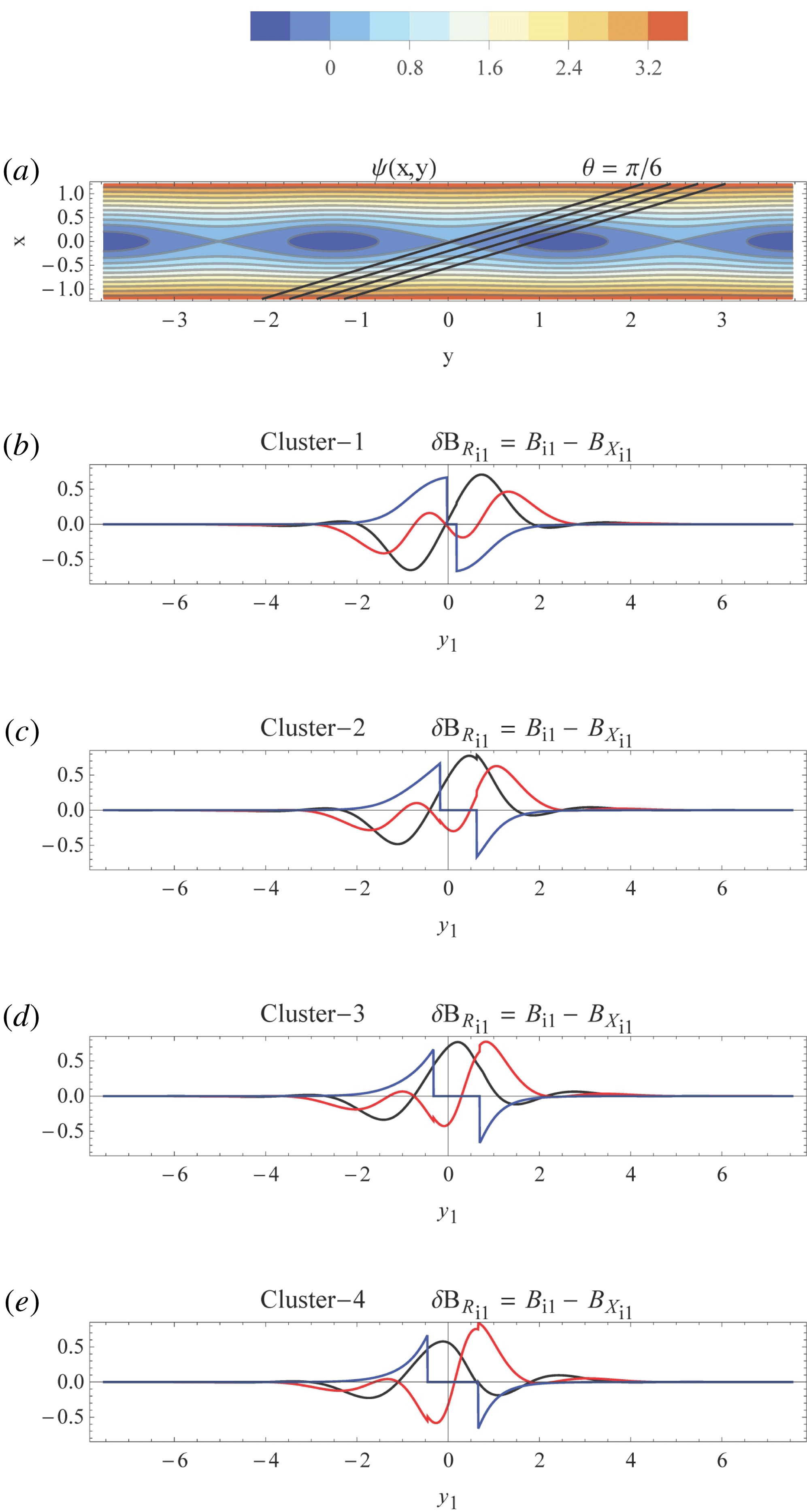
(a) “Cat’s eyes”. The contour plot (colour legend on top) of the vector potential
 $\unicode[STIX]{x1D713}$
, see (3.1) and (3.7). The parameters are chosen as
 $A=1.6$
,
 $\unicode[STIX]{x1D705}=2.5$
,
 $\unicode[STIX]{x1D6FE}=0.2$
and
 $\unicode[STIX]{x1D70E}=0.4$
. Four black parallel lines represent the trajectories of four spacecraft, C1–C4 (from left to right). (b–e) Rapid magnetic field
 $\unicode[STIX]{x1D6FF}\boldsymbol{B}_{R}=\unicode[STIX]{x1D735}\times \boldsymbol{e}_{z}(\unicode[STIX]{x1D713}-\unicode[STIX]{x1D713}_{X})+\boldsymbol{e}_{z}\unicode[STIX]{x1D6FF}B_{z}$
, as would be recorded by four observers (‘Cluster satellites’) travelling along the trajectories indicated by parallel black lines in the first panel, with the typical parameters: distance between trajectories
 $\unicode[STIX]{x0394}d=0.15$
; angle to the chain’s axis
 $\unicode[STIX]{x1D703}=\unicode[STIX]{x03C0}/6$
. The
 $x1$
,
 $y1$
, and
 $z$
components of the rapid magnetic field are displayed in black, red and blue, respectively. The normalizations are given in (2.9).

Our results can be used to explain the structures observed in and around the current sheets in space plasmas, e.g. in the slow and the fast solar winds, planetary magnetosheaths, etc. They are displayed in figure 1, in a form that mimics the measurements made by four observers moving along straight lines that intersect the magnetic chain at the angle
 $\unicode[STIX]{x1D703}$
. We used the following set of typical dimensionless parameters:
 $A=1.6$
,
 $\unicode[STIX]{x1D705}=2.5$
,
 $\unicode[STIX]{x1D6FE}=0.2$
,
 $\unicode[STIX]{x1D70E}=0.4$
. The distance between neighbouring satellite trajectories is taken as
 $\unicode[STIX]{x0394}d=0.15$
and their angle to the chain’s axis
 $\unicode[STIX]{x1D703}=\unicode[STIX]{x03C0}/6$
. Furthermore, for an easier comparison with the Cluster observations described in § 4 below, we plot our results in the ‘solar wind reference frame’ i.e. we decompose the magnetic field obtained from (3.1) and (3.7) into components that are parallel and perpendicular to an arbitrary vector
 $\boldsymbol{V}_{\bot }$
perpendicular to the background magnetic field
 $B_{0}\boldsymbol{e}_{z}$
, viz.
 $\unicode[STIX]{x1D6FF}B_{R_{y1}}=\boldsymbol{e}_{V_{\bot }}\boldsymbol{\cdot }[\unicode[STIX]{x1D735}\times \boldsymbol{e}_{z}(\unicode[STIX]{x1D713}-\unicode[STIX]{x1D713}_{X})]$
and
 $\unicode[STIX]{x1D6FF}B_{R_{x1}}=\boldsymbol{e}_{V_{\bot }}\boldsymbol{\cdot }\unicode[STIX]{x1D735}(\unicode[STIX]{x1D713}-\unicode[STIX]{x1D713}_{X})$
. Here
 $\boldsymbol{V}_{\bot }$
denotes the solar wind velocity component perpendicular to the background magnetic field,
 $\boldsymbol{e}_{V_{\bot }}$
is a unit vector
 $\boldsymbol{e}_{V_{\bot }}=\boldsymbol{V}_{\bot }/|\boldsymbol{V}_{\bot }|$
, and
 $\unicode[STIX]{x1D713}_{X}(x)$
is the background, or the envelope vector potential (denoted in § 4 as the ‘1 s average’), given by
 $\unicode[STIX]{x1D713}_{X}(x)=A\log [(\cosh \unicode[STIX]{x1D705}x+\unicode[STIX]{x1D6FE})/(1+\unicode[STIX]{x1D6FE})]$
(see (3.1)). Parallel magnetic field perturbation
 $\unicode[STIX]{x1D6FF}B_{z}$
is given by (2.10).
4 Cluster observations
As an illustrative example, we present results of satellite observations that are conformal with our structure (3.6)–(3.7), albeit not being of an exceedingly large size, viz.
 $c^{2}\unicode[STIX]{x1D6FB}_{\bot }^{2}/\unicode[STIX]{x1D714}_{pi}^{2}\sim 0.1{-}0.25$
. The measurements were done in the slow solar wind in the time interval analysed also in Perrone et al. (Reference Perrone, Alexandrova, Mangeney, Maksimovic, Lacombe, Rakoto, Kasper and Jovanovic2016), using the fluxgate magnetometer (FGM) and the Spatio Temporal Analysis of Field Fluctuations experiment (STAFF) on board the Cluster satellites, whose description is given in Balogh et al. (Reference Balogh, Carr, Acuña, Dunlop, Beek, Brown, Fornaçon, Georgescu, Glassmeier and Harris2001), Cornilleau-Wehrlin et al. (Reference Cornilleau-Wehrlin, Chanteur, Perraut, Rezeau, Robert, Roux, de Villedary, Canu, Maksimovic and de Conchy2003). A detailed explication of the measurements will be given in a separate publication, and here we present only those data that are relevant for our present study. The observed magnetic structures, detected as in Alexandrova et al. (Reference Alexandrova, Mangeney, Maksimovic, Cornilleau-Wehrlin, Bosqued and André2006), Alexandrova & Saur (Reference Alexandrova and Saur2008), are displayed in figures 2–4. They feature a gentle ramp in the magnetic field intensity
 $|\boldsymbol{B}|-\langle |\boldsymbol{B}|\rangle _{10\,\text{s}}$
, where
 $\langle \cdots \rangle _{\unicode[STIX]{x1D70F}}$
denotes the moving average over the period
 $\unicode[STIX]{x1D70F}$
, viz.
 $\langle f(t)\rangle _{\unicode[STIX]{x1D70F}}=\int _{t-\unicode[STIX]{x1D70F}/2}^{t+\unicode[STIX]{x1D70F}/2}\,\text{d}t^{\prime }\,f(t^{\prime })$
. The average strength of the magnetic field was evaluated adopting
 $\unicode[STIX]{x1D70F}=10~\text{s}$
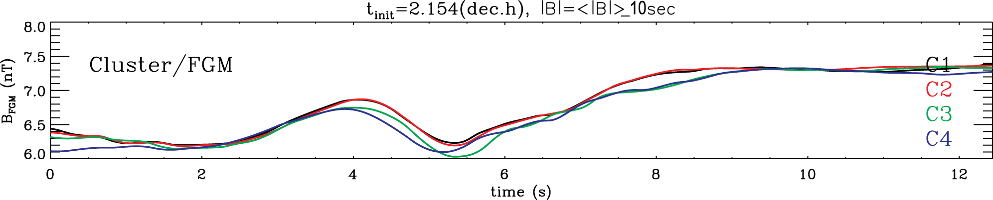
. An approximatively linear growth by 25 % (from
 ${\sim}6$
to
 ${\sim}7.5~\text{nT}$
) in the course of
 ${\sim}4~\text{s}$
was observed. The velocity of the slow solar wind was
 $V\sim 330~\text{km}~\text{s}^{-1}$
while the velocity of the structures was calculated from the time delay between the signals recorded on the four spacecraft. It was established that the structures were mostly carried by the solar wind, since using two different methods their velocity in the plasma frame was determined to be
 $18\pm 32~\text{km}~\text{s}^{-1}$
and
 $-3\pm 32~\text{km}~\text{s}^{-1}$
, respectively. Likewise, from the comparison between the signals, it was estimated that their characteristic length in the direction perpendicular to their propagation was considerably bigger than the distance between satellites. Taking that the average magnetic field
 $\langle \boldsymbol{B}\rangle _{10\,\text{s}}$
is frozen into the solar wind and carried by it with velocity
 $\boldsymbol{V}$
, where
 $|\boldsymbol{V}|\sim 330~\text{km}~\text{s}^{-1}$
, the length of the ramp is estimated to be
 ${\sim}1500~\text{km}$
, which corresponds to
 ${\sim}30$
ion plasma lengths (
 $c/\unicode[STIX]{x1D714}_{p,i}\sim 50~\text{km}$
). From the raw satellite data, the variations of the magnetic field were determined on the (relatively) short and long temporal scales of
 $\unicode[STIX]{x1D70F}=1~\text{s}$
and
 $\unicode[STIX]{x1D70F}=10~\text{s}$
, respectively. The rapid part of the magnetic field
 $\unicode[STIX]{x1D6FF}\boldsymbol{B}_{R}$
is defined as
 $\unicode[STIX]{x1D6FF}\boldsymbol{B}_{R}=\boldsymbol{B}-\langle \boldsymbol{B}\rangle _{1\,\text{s}}$
, and the slow part
 $\unicode[STIX]{x1D6FF}\boldsymbol{B}_{S}$
as
 $\unicode[STIX]{x1D6FF}\boldsymbol{B}_{S}=\boldsymbol{B}-\langle \boldsymbol{B}\rangle _{10\,\text{s}}$
.
The variation of the magnetic field intensity
 $|\boldsymbol{B}|$
. Data recorded by the four Cluster satellites C1–C4 are displayed as black, red, green and blue lines, respectively.

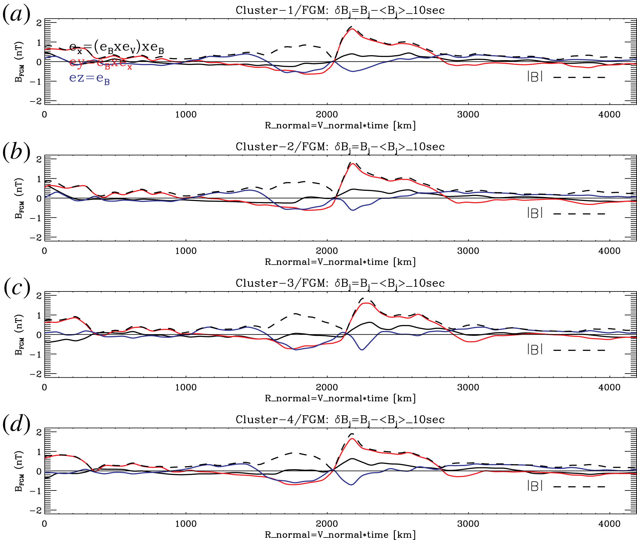
Slow variation of the magnetic field,
 $\unicode[STIX]{x1D6FF}\boldsymbol{B}_{S}$
, i.e. the deviation of the magnetic field from its 10 s average,
 $\unicode[STIX]{x1D6FF}\boldsymbol{B}_{S}=\boldsymbol{B}-\langle \boldsymbol{B}\rangle _{10~\text{s}}$
. The
 $x$
,
 $y$
and
 $z$
components are displayed in black, red and blue, respectively. From top to bottom: data from the Cluster spacecraft C1–C4.

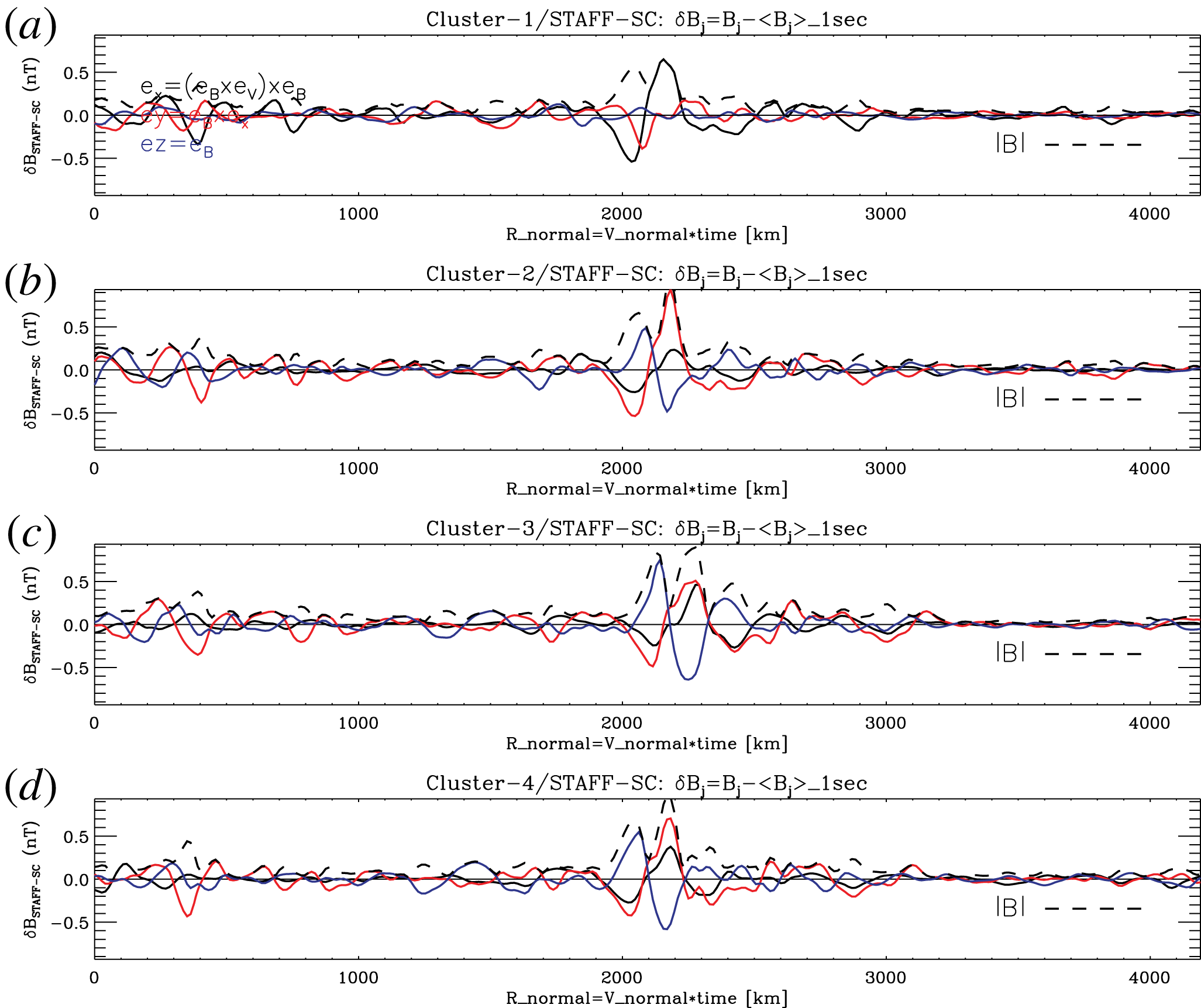
Rapid variation of the magnetic field,
 $\unicode[STIX]{x1D6FF}\boldsymbol{B}_{R}$
, i.e. the deviation of the magnetic field from its 1 s average,
 $\unicode[STIX]{x1D6FF}\boldsymbol{B}_{R}=\boldsymbol{B}-\langle \boldsymbol{B}\rangle _{1\,\text{s}}$
. The
 $x$
,
 $y$
and
 $z$
components are displayed in black, red and blue, respectively. (a–d) Data from the Cluster spacecraft C1–C4.

These data are displayed in figures 3 and 4, for each of the Cluster spacecraft. The local, time-independent, Cartesian reference frame used in these figures (the ‘solar wind frame’) is defined as follows. Its
 $z$
-axis is adopted to be parallel to the magnetic field, averaged over the entire period of observation that lasted 12 s, the
 $y$
-axis is taken to be perpendicular both to
 $\langle \boldsymbol{B}\rangle _{12\,\text{s}}$
and to the direction of the solar wind, while the
 $x$
-axis is oriented along the solar wind velocity component
 $\boldsymbol{V}_{\bot }$
that is perpendicular to the average magnetic field
 $\langle \boldsymbol{B}\rangle _{12\,\text{s}}$
, viz.
 $$\begin{eqnarray}\displaystyle \boldsymbol{e}_{z}=\langle \boldsymbol{B}\rangle _{12\,\text{s}}/|\langle \boldsymbol{B}\rangle _{12\,\text{s}}|,\quad \boldsymbol{e}_{y}=\boldsymbol{e}_{z}\times \boldsymbol{V}/|\boldsymbol{V}|,\quad \boldsymbol{e}_{x}=\boldsymbol{e}_{y}\times \boldsymbol{e}_{z}. & & \displaystyle\end{eqnarray}$$
We note from figures 3 and 4 that during the entire period of observations
 $0\leqslant t\leqslant 12~\text{s}$
, the slow magnetic field
 $\unicode[STIX]{x1D6FF}\boldsymbol{B}_{S}$
featured a very small (
 ${\lesssim}5\,\%$
) linear growth of its parallel component,
 $\unicode[STIX]{x1D6FF}B_{S_{z}}$
. Conversely, its perpendicular components
 $\unicode[STIX]{x1D6FF}B_{S_{x}}$
and
 $\unicode[STIX]{x1D6FF}B_{S_{y}}$
exhibited broad maxima and minima with mostly flat tops and bottoms and with a rather abrupt change of sign at
 $t\simeq 6~\text{s}$
. The slow magnetic field
 $\unicode[STIX]{x1D6FF}\boldsymbol{B}_{S}$
is mostly perpendicular to the solar wind, since
 $\unicode[STIX]{x1D6FF}B_{S_{y}}>\unicode[STIX]{x1D6FF}B_{S_{x}},\unicode[STIX]{x1D6FF}B_{S_{z}}$
. All three components of the rapid magnetic field
 $\unicode[STIX]{x1D6FF}\boldsymbol{B}_{R}$
exhibit similar profiles, with a relatively narrow minimum and maximum with the widths
 $\unicode[STIX]{x0394}t\sim 1~\text{s}$
(i.e.
 ${\sim}330~\text{km}$
), and a rapid change of sign at
 $t\simeq 6~\text{s}$
(2000 km). The magnitudes of the particular minima and maxima at various Cluster spacecraft are, to some degree, quantitatively different. We note that the perpendicular components of the slow and rapid magnetic fields are not parallel to each other, since
 $\unicode[STIX]{x1D6FF}B_{S_{x}}/\unicode[STIX]{x1D6FF}B_{S_{y}}\neq \unicode[STIX]{x1D6FF}B_{R_{x}}/\unicode[STIX]{x1D6FF}B_{R_{y}}$
, which suggests a two-dimensional geometry of the latter. Large-scale sheared flows were not observed, but the small resolution and small sampling rate of their instruments could not exclude the existence of undetected short-scale plasma flows.
As a reasonable model for these observations, in the preceding section we assumed that the background plasma flow was asymptotically equal to zero, while the shape of the perpendicular slow magnetic field
 $\unicode[STIX]{x1D6FF}B_{S_{x}}$
,
 $\unicode[STIX]{x1D6FF}B_{S_{y}}$
was modelled by infinitely stretching its broad maxima and minima to a
 ${\sim}\text{tanh}$
shape, see (3.2). A qualitative agreement of our theoretical predictions, displayed in figure 1, with the observations is apparent. Notably, the components
 $\unicode[STIX]{x1D6FF}B_{R_{x1}}$
and
 $\unicode[STIX]{x1D6FF}B_{R_{y1}}$
feature mostly asymmetric bipolar signals, very similar to the satellite observations in figure 4. For larger angles
 $\unicode[STIX]{x1D703}$
(
 $\unicode[STIX]{x1D703}\gtrsim \unicode[STIX]{x03C0}/4$
), the multiple maxima/minima vanish and we observe only asymmetric bipolar signals, which in a limited number of events degenerate into monopolar. However, many relevant parameters of the satellites’ encounters with the structure are not known, such as the angle between the structure and the solar wind, ratio of the chain’s longitudinal and perpendicular scale lengths, the relative position of the satellites to the structure’s
 $x$
-point, etc. Furthermore, a statistical analysis cannot be performed since only a small number of encounters have been recorded. Thus, an exact one-to-one quantitative matching between our theoretical predictions and the observational data is not possible to present here.
5 Concluding remarks
We have constructed a coherent stationary nonlinear solution of the Kadomtsev–Pogutse–Strauss equations of reduced MHD that satisfy the asymptotic boundary conditions observed by the Cluster spacecraft in the high-
 $\unicode[STIX]{x1D6FD}$
plasma of the slow solar wind close to the Earth. An analytic cat’s eyes-type solution is found in the form of a chain of magnetic vortices that is imbedded in a sheared magnetic field and in a localized laminar plasma flow. It possesses a significant compressional component of the magnetic field and traps the plasma fluid inside its magnetic separatrix. Such structure could have been created either in the turbulence cascade together with the current sheet in which it is imbedded, or it constitutes the signature of a past reconnection event. The apparent singularity of our solution is naturally resolved on the electron spatial scale, but it is also suppressed when a smooth nonlinear model function (3.5) is used instead of the applied simple part-by-part linear function suitable for analytic calculations. At the magnetic separatrix, the latter gives rise to a current sheet and/or a plasma jet whose widths are finite and determined by the parameter
 $\unicode[STIX]{x1D6F9}$
, which can be seen in (3.6). However, it should be noted that the measurements of the plasma flow from Cluster spacecraft were performed with a relatively low resolution. Based on such relatively poor observational data available at present time, we are able to assert only the absence of significant large-scale flows associated with the magnetic structures in figures 2–4. Since, due to the low resolution, it was not possible to resolve the short-scale plasma flows, it is quite likely that the anticipated current sheet and/or plasma jet located at the separatrix of our cat’s eyes solution would remain undetected.
An exact one-to-one quantitative matching between our theoretical predictions and the observational data is not possible to present here, because many relevant parameters of the satellites’ encounter with the structure are not known and only a small number of encounters are recorded which does not provide sufficient data for statistical analysis. However, a striking qualitative agreement between them is apparent. Notably, the components
 $\unicode[STIX]{x1D6FF}B_{x1}$
and
 $\unicode[STIX]{x1D6FF}B_{y1}$
feature mostly asymmetric bipolar signals, very similar to the satellite observations in figure 4. For larger angles
 $\unicode[STIX]{x1D703}$
(
 $\unicode[STIX]{x1D703}\gtrsim \unicode[STIX]{x03C0}/4$
), the multiple maxima/minima vanish and we observe only asymmetric bipolar signals, which in a limited number of events degenerate into monopolar. Their small but visible discontinuities in figure 1, occurring at the magnetic separatrix, result from our choice of a part-by-part linear function
 $F(\unicode[STIX]{x1D713})$
and are readily removed by the use of a smooth model function, equation (3.5). Notwithstanding its discontinuity (more pronounced than that of
 $\unicode[STIX]{x1D6FF}B_{x_{1}}$
and
 $\unicode[STIX]{x1D6FF}B_{y_{1}}$
because it involves higher derivatives of the potential) that definitely vanishes when a smooth function
 $F(\unicode[STIX]{x1D713})$
is used, our solution for
 $\unicode[STIX]{x1D6FF}B_{z}$
features the parity and the spatial scaling that are in good agreement with the observations.
Acknowledgements
This work was supported in part (D.J. and M.B.) by the MPNTR 171006 and NPRP 8-028-1-001 grants. D.J. acknowledges financial support from the Observatoire de Paris and of the French CNRS, and the hospitality of the LESIA laboratory in Meudon.