Introduction

Amid many efforts to better simulate 21st-century Arctic sea-ice decline, there is a growing impetus within the scientific community to resolve modeled polar oceanic and atmospheric physics that are contingent upon high spatial resolution land-atmosphere (˂50km) and ice-ocean (˂1/10°) models (Reference Maslowski, Clement Kinney, Higgins and RobertsMaslowski and others, 2012). Many Earth System Models cited in the latest Intergovernmental Panel on Climate Change (IPCC) Assessment Report (Reference Stocker and GroupStocker and others, 2013) do not resolve these scales and are therefore unable to simulate mesoscale Arctic storms, high-latitude oceanic eddies, narrow Arctic boundary currents, oceanic tides or linear kinematic features in sea ice. These are only a few examples from a long list of polar processes and physics contingent upon high spatial resolution, the importance of which remains to be fully investigated for their impact on simulated polar climate. Notwithstanding, evidence from stand-alone atmosphere and ice-ocean models, as well as observations, indicates that such processes increase local sub-daily variance within the polar environment, with expected energy cascades to climatic timescales (e.g. Reference Holloway and ProshutinskyHolloway and Proshutinsky, 2007; Reference Maslowski, Kinney, Marble, Jakacki, Hecht and HasumiMaslowski and others, 2008; Reference DuVivier and CassanoDuVivier and Cassano, 2013). Coupled processes that are primarily contingent upon high temporal resolution have often received less attention in Earth System Models, and in this paper we focus on one such physical interaction in the polar oceans: inertial oscillations in sea ice, which may be considered a proxy for transient Ekman transport in the ice-ocean boundary layer (Reference Heil and HiblerHeil and Hibler, 2002; Reference Hibler, Roberts, Heil, Proshutinsky, Simmons and LovickHibler and others, 2006).

There is a dearth of literature on the simulation of ice-ocean inertial oscillations in fully coupled Earth System Models, partly because they are difficult to evaluate in global climate models using only short buoy records. Simulating them requires frequent (^hourly) atmosphere-ice-ocean flux exchange, which can be computationally restrictive. For example, the Community Earth System Model (CESM; Reference HurrellHurrell and others, 2013) exchanges time-averaged oceanic fluxes at daily intervals (following Reference GentGent and others, 2011), which naturally filters semi-diurnal feedbacks between ice, ocean and the atmosphere, removing the oscillatory Ekman transport signal from interfacial ice-ocean stress. By contrast, some of the best sea-ice simulations in the recent Coupled Model Intercomparison Project (CMIP5) were from the ACCESS model (Reference Stocker and GroupStocker and others, 2013) which includes ice-ocean flux exchange at hourly or half-hourly intervals (Reference BiBi and others, 2013). A direct result of less frequent coupling is that ice-ocean Ekman transport is damped, even though the sea-ice and ocean models may represent inertial oscillations internally. In this paper, we aim to demonstrate the importance of frequent atmosphere-ice-ocean coupling in simulating polar Ekman transport using two fully coupled models. We evaluate established sea-ice and ocean codes in a fully coupled regional climate model against observations of inertial oscillations in sea ice. We then apply guidance from this work in a new CESM configuration to assess the effect of high-frequency coupling on simulated transient ice-ocean Ekman transport in the Arctic and Southern Ocean. To place this work in context, it is useful to first review prominent modeling and observational analysis that has heretofore advanced our understanding of this topic.

Transient Ice–Ocean Ekman Transport

Following Reference McPhee and NewMcPhee (1978), Reference Heil and HiblerHeil and Hibler (2002) and Reference Hibler, Roberts, Heil, Proshutinsky, Simmons and LovickHibler and others (2006), and neglecting advective acceleration, evolution of the combined, idealized ice-ocean Ekman transport, Me, may be described as

(1)

where テ_a is the surface wind stress vector, f is the Coriolis parameter, k is the unit vector normal to the sea surface and σ_{m n} is the internal sea-ice stress tensor (m,n = 1,2) resulting from sea-ice velocity in the absence of geostrophic flow for time t. Neglecting snow accumulated on the surface of sea ice, the combined ice-ocean Ekman transport can be expressed as the sum of ice and ocean components:

(2)

where p is density, _e is the Ekman component of the boundary layer ice-ocean velocity, hi is sea-ice thickness, z is ocean depth, and subscripts i and o denote sea ice and ocean, respectively. Equation (1) describes a forced harmonic oscillator damped by internal ice stress, which is dependent upon sea-ice concentration and thickness. As they decrease, σ_mn σ_mn declines nonlinearly (e.g. Reference Thorndike, Rothrock, Maykut and ColonyThorndike and others, 1975; Reference HiblerHibler, 1980; Reference Bitz, Holland, Weaver and EbyBitz and others, 2001). When internal ice stress is negligible, Eqn (1) reduces to a second-order inhomogeneous partial differential equation, for which the analytic solution demonstrates that M traces a clockwise perfect local circle with a period σ_mn ranging from approximately 11.96 to 17 hours in the Northern Hemisphere sea-ice zone, and 12.21 to 14.60 hours in the Southern Hemisphere sea-ice zone. By virtue of Eqn (2), the Ekman component of sea-ice velocity, ie, rotates in phase with and has a magnitude proportional to M, and may therefore be measured as a proxy for ice-ocean Ekman transport and used as an indicator of stress-induced mixing in the ice-ocean boundary layer.

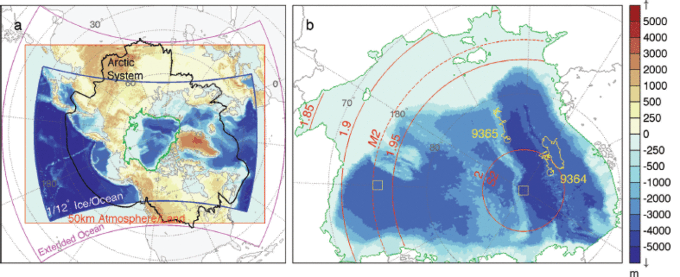
Inertial oscillations have been measured in Arctic and Southern Ocean sea ice using a variety of techniques. They are typically excited by impulsive wind forcing or internal ice stress (e.g. Reference HunkinsHunkins, 1967; Reference HiblerHibler and others, 1998; Reference KwokKwok and others, 2003; Reference Geiger and PerovichGeiger and Perovich, 2008; Reference MeierMcPhee, 2008; Leppäranta and others, 2012), especially during the passage of storms over polar oceans (e.g. Reference Lammert, Brummer and KaleschkeLammert and others, 2009). However, up until the routine use of GPS locations in the International Arctic Buoy Program (IABP) from ∼2005 onwards, the extent to which inertial oscillations affect basin-scale sea-ice deformation, growth and melt was unclear. However, evidence is emerging of climatic changes in inertial oscillations in sea ice attributable to mechanical weakening of the pack (Reference Gimbert, Jourdain, Weiss and BarnierGimbert and others, 2012a). Inertial oscillations in sea ice interfere with tidal waves in polar oceans at certain latitudes (e.g. Fig. 1), and provide a source of ocean surface stress for the generation of near-inertial waves that disperse downward and horizontally in the ocean (e.g. Reference Guthrie, Morison and FerGuthrie and others, 2013). This has important implications for our understanding of the seasonality of oceanic mixing in polar oceans.

Fig. 1.

Configuration of the Regional Arctic System Model and the central Arctic analysis region used in this study. (a) Boundaries of the ice-ocean domain (blue outline and resolved bathymetry), the atmosphere-land domain boundary (red) and the extended ocean domain (magenta). Topographic and bathymetric pixels (shading) represent single model gridcells on the 50 km atmosphere-land and ∼9 km ice-ocean domains, respectively. The Arctic System boundary indicates the area north of the 1990-99 mean 10°C sea surface and surface air 0°C isotherms that encircle the North Pole, and the southern limit of terrain that drains into the High Arctic as defined in Reference RobertsRoberts and others (2010). The area encircled by the green line represents the central analysis domain used for the RASM case study in this paper, which is enlarged in (b). (b) The yellow buoy tracks and end-point circles indicate the track of IABP drifters 9364 and 9365 for the year 1996 as used by Reference Heil and HiblerHeil and Hibler (2002). Yellow boxes show the location of time-series analysis for the Community Earth System Model in Figure 11. Red contours indicate the inertial frequency (d-¹), and the latitudes at which M2 and S2 tidal oscillations share the inertial frequency.

Global and hemispheric studies of the contribution of inertia to oceanic mixing have heretofore neglected polar areas (e.g. Reference Park, Kim and KingPark and others, 2005, Reference Park, Kim and Schmitt2009) or do not explicitly address complications relating to sea-ice cover (e.g. Reference Rath, Greatbatch and ZhaiRath and others, 2014), partly because of a lack of observations. However, some measurements of enhanced oceanic mixing resulting from Ekman pumping induced by sea-ice mechanics or from a reduced ice cover exist for the Beaufort Sea (e.g. Rainville and Woodgate, 2009; Reference Dosser, Rainville and TooleDosser and others, 2014). A number of modeling studies have investigated the impact of inertial oscillations on sea-ice drift and deformation in the Arctic, including Reference McPhee and NewMcPhee (1978), Reference Heil and HiblerHeil and Hibler (2002) and Reference Hibler, Roberts, Heil, Proshutinsky, Simmons and LovickHibler and others (2006). Related work to ‘embed’ sea ice in baroclinic ocean models has helped to improve the barotropic mode of which Ekman transport is a component (e.g. Reference Campin, Marshall and FerreiraCampin and others, 2008; Reference GriffiesGriffies, 2010). Much of the analysis of so called ‘high-frequency ice-ocean dynamics’ in models has been confined to stand-alone ice-ocean simulations and there are few studies addressing the relevant physics in fully coupled climate models. Previous stand-alone ice-ocean Arctic modeling studies have typically used 6 hourly interpolated wind forcing from reanalyses, which causes unavoidable complications: The driving wind stress contains an alias at the Nyquist frequency (v/ = 2 d-¹), artificially exciting the Ekman layer in a latitudinal band surrounding 85°N sin^-1(vπΩ), given Earth’s angular frequency of rotation Ω=6.3042 rad d-¹. Direct linear forcing of the Ekman layer north of this latitude is neglected, including a considerable tract of the Transpolar Drift. Use of an anti-alias filter to avert the aliasing only expands the region around the North Pole without linear forcing at the resonant frequency of the system, due to loss of wind stress power near and at the Nyquist frequency. As a result it has been difficult to assess the relative basin-wide contribution of nonlinear sea-ice mechanics and direct linear wind forcing of the ice-ocean boundary layer prior to the availability of 3 hourly reanalysis data. Use of 3 hourly reanalysis fields averts this problem but still neglects high-frequency feedbacks with the atmosphere (e.g. Reference Gimbert, Jourdain, Weiss and BarnierGimbert and others, 2012a), preventing a full assessment of the contribution of Ekman transport to variance within the atmosphere-ice-ocean boundary layer system.

In this paper, we present an inertial oscillation case study based on results from a fully coupled model that allows coupled feedbacks not present in stand-alone ice-ocean simulations, and also facilitates validation methods not possible in global models. The Regional Arctic System Model (RASM) used in this study is a fully coupled high-resolution climate model that comprehensively resolves the ice-ocean inertial period. Because RASM is fully coupled, it negates the aforementioned problems of aliasing and low-pass filtration of surface fluxes. In previous research in stand-alone ice-ocean models, high-frequency Arctic Ocean dynamics have addressed diurnal tidal interaction as well as inertial oscillations (e.g. Reference Hibler, Roberts, Heil, Proshutinsky, Simmons and LovickHibler and others, 2006; Reference ChenChen and others, 2009), but here we limit our fully coupled model analysis to the latter and confine our study prior to the onset of the rapid decline of perennial Arctic sea-ice volume in the past decade. The aim of our investigation is to isolate the ice-ocean Ekman transport signal in a single RASM realization and gain an understanding of its simulated basin-wide seasonal progression. Because RASM is regionally constrained, it facilitates model evaluation using daily observations for a specific year in the climate record. This is prohibitive in global coupled models because global internal variability restricts the minimum time window over which Earth System Models can be compared with observations, depending on ensemble size. But here we can use RASM as a fully coupled framework to evaluate ice-ocean Ekman transport. We then apply to CESM the methods evaluated in RASM to demonstrate how changes in ice-ocean coupling affect Ekman transport in one prominent global model cited in the latest IPCC (Reference Stocker and GroupStocker and others, 2013) report.

The Regional Arctic System Model

RASM is a limited-area, fully coupled atmosphere-ice-ocean-land model consisting of the Weather Research and Forecasting (WRF) model, Los Alamos National Laboratory (LANL) Parallel Ocean Program (POP) and Sea Ice Model (CICE) and the Variable Infiltration Capacity (VIC) land hydrology model. RASM is configured on the pan-Arctic domain displayed in Figure 1a, and covers the entire Northern Hemisphere marine cryosphere, terrestrial drainage to the Arctic Ocean, major inflow and outflow pathways, with extension into the North Pacific and Atlantic oceans to account for the passage of cyclones into the Arctic. WRF and VIC share a 50 km resolution polar stereographic mesh, and POP and CICE share a 1/12° rotated sphere grid with the equator passing through the North Pole. This provides a horizontal ice-ocean resolution of ∼9 km across the Arctic Ocean, which is eddy-permitting across the entire domain. An extended ocean domain surrounds the boundaries of the POP/CICE mesh to pass observed surface boundary conditions to WRF where the atmospheric mesh extends beyond the ocean model’s lateral boundaries, similar to the method used by Reference DornDorn and others (2007). A major advantage of this RASM configuration is that there are no native poles on any of the model grids, avoiding significant grid convergence that can arbitrarily filter waves in high-latitude simulations. Table 1 summarizes the discretization within each component model.

Table 1.

Spatial and temporal resolution of the Regional Arctic System Model as used in this study

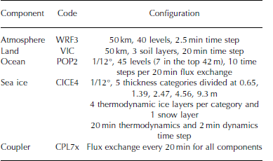
RASM in this study uses the same sea-ice and ocean models (CICE and POP) as CESM Version 1.1. Most relevant to this research is the sea-ice dynamics configuration, which uses the elastic-viscous-plastic (EVP) rheology as first described by Reference Hunke and DukowiczHunke and Dukowicz (1997) and subsequently updated, as summarized in Reference Hunke, Lipscomb and LosHunke and Lipscomb (2010). RASM uses five sea-ice thickness categories to represent compressive sea-ice strength as indicated in Table 1, assuming isostasy following Reference RothrockRothrock (1975) but with an exponential ridged ice thickness distribution (Reference Lipscomb, Hunke, Maslowski and JakackiLipscomb and others, 2007) and ∼94% of kinetic energy lost to friction during ridge building. A variable atmospheric drag coefficient is calculated over sea ice following Reference Brunke, Zhou, Zeng and AndreasBrunke and others (2006), in combination with a constant ice-ocean drag coefficient of C _o = 0.00536. Further details of this coupling are provided in Appendix A, which describes how the Polar Science Center Hydrographic Climatology (PHC) is used for prescribed oceanic boundary conditions.

Coupling of all RASM components is based on the same flux coupler as CESM Version 1.1, denoted as CPL7 (Reference Craig, Vertenstein and JacobCraig and others, 2012). However, for this study, CPL7 has undergone significant modifications especially relevant to high-frequency sea-ice motion. In particular, we have modified the coupling sequence to ensure there is no more than one coupling time-step lag between the sea-ice and ocean models. Coupled models inherently possess lags, which can cause instabilities if these lags become too great relative to the period of the signals within the coupled system. Therefore it is important to model ice-ocean Ekman transport so that the lag between i_e and _oe in Eqn (2) is as small as possible. Our new version of CPL7, which we denote CPL7x, ensures this is the case when using the standard RASM 20min coupler step. This satisfies idealized Kuramoto stability criteria (e.g. Reference Mirollo and StrogatzMirollo and Strogatz, 2005) for two coupled oscillators pulsing at the same inertial frequency within sea-ice zones. It also satisfies the Reference HallbergHallberg (2014) stability equations for ice-ocean models. The 20 min coupling in RASM ensures a coupling phase lag of ∼10° or less between _i e and _oe, and ∼15° or less for the 30min high-frequency CESM coupling used in this paper.

Details on the atmosphere and land model configurations in RASM may also be found in Appendix A. Most important to this work is that we spectrally nudge WRF to ERA-Interim reanalyses (Reference DeeDee and others, 2011) above 500 hPa up to wavenumbers 4 and 3 on the abscissa and ordinate axes, respectively, of the WRF domain (Fig. 1a). The limits of wavenumber nudging are proportional to the relative lengths of the axes. We nudge the temperature and wind with a strength of 0.0003 (see Reference SkamarockSkamarock and others, 2008, for information about the precise physical meaning of this parameter). This configuration allows the atmosphere-ice-ocean boundary layer system to freely evolve under the constraint of large-scale upper atmospheric circulation, including the polar vortex, consistent with the 6 hourly ERA-Interim lateral boundary conditions used in this study.

Ice-Ocean Ekman Transport in the Regional Arctic System Model

Regional coupled models provide a platform for detailed model evaluation against daily measurements while including coupled atmospheric feedbacks. Using RASM as a fully coupled climate evaluation platform, we focus here on its ability to simulate inertial oscillations in sea ice and compare the results with daily observations. We have confined our RASM case study to 1996 and our analysis to the central Arctic region shown in Figure 1b. The case-study year pre-dates the 21st-century rapid decline of summer Arctic sea-ice extent, and can be compared with previously published modeling results on Arctic inertial oscillations by Reference Heil and HiblerHeil and Hibler (2002). We initialized our RASM simulation, herein referred to as RASMe1, on 1 September 1989 and ran the model to the end of 1996. The land and ice-ocean components are initialized with spun-up states from their respective stand-alone versions forced respectively with ERA-Interim and CORE-2 reanalyses (Reference Large and YeagerLarge and Yeager, 2008). WRF was initialized with ERA-Interim at the start of September 1989.

To evaluate the domain-wide performance of RASMe1, we use a passive microwave climate data record (CDR) of sea-ice extent and area as described by Reference MeierMeier (2013). In comparing with the CDR, we have filtered for sea ice less than 0.3 m in the thinnest model category, reflecting the likely underestimation of ice concentration in the marginal ice zone when measured using passive microwave techniques (e.g. Reference KarvonenKarvonen, 2014). The model overestimates sea-ice extent in light of this uncertainty (Fig. 2), but this is of little consequence for the central Arctic analysis region.

Fig. 2.

Model-observation comparison of sea-ice (a) extent, (b) area and (c) thickness, for RASMe1 (red). Extent is limited to ice categories ˃0.3 m thick for comparison against the passive microwave climate data record. The ice area comparison avoids the gap in Special Sensor Microwave/Imager (SSM/I) retrievals surrounding the North Pole.

We also evaluated the surface geostrophic wind field against 3 monthly ERA-Interim averages. The model surface atmospheric circulation does not possess any substantial semi-decadal bias relative to ERA-Interim reanalyses (Fig. 3). As a result, we are able to isolate discrepancies in simulated sea-ice drift (Fig. 4) to factors other than surface wind field bias, something that is not readily possible in fully coupled global simulations. Increased cyclonic activity over the pack between July and September (Fig. 3) reflects in a disruption of the Beaufort Gyre and Transpolar Drift during summer (Fig. 4). During July-September, a mean cyclonic wind circulation pattern develops that is centered over the North Pole, corresponding to a greater number of low-pressure systems traversing the central Arctic in summer.

Fig. 3.

Mean seasonal surface geostrophic wind on the RASM atmospheric model domain, indicating low wind-forcing bias over sea ice. Red streamlines represent the RASMe1 surface flow for 1992-96, and blue streamlines represent the corresponding ERA-Interim circulation. Successive 3 month averages (a-d) correspond to the same time periods in Figure 4a-d. The black coastal boundary indicates the division along which the 1/12° POP/CICE grid projects a surface type of 50% land and 50% sea ice or ocean onto the lower-resolution 50 km WRF mesh.

Fig. 4.

Mean central Arctic sea-ice thickness (shading) and drift (vectors) for RASMe1 during 1992–96 (a–d) and 1996 only (e–h) wherever model concentration exceeds 15%. Each vector represents a mean of 256 model gridcell velocities, masked for land. The comparable climate data record sea-ice extent is shown in magenta. Navy-blue traces indicate the seasonal drift track of IABP buoys 9364 and 9365 as indicated in Figure 1b and corresponding to their respective times of operation. Boxes are positioned on the end buoy position for the 1996 3 month windows indicated for each frame.

Given these broad model statistics, RASM sea-ice velocity is evaluated against 3 hourly sea-ice drift derived from GPS locations of two 1996 IABP drifters in the Amundsen Basin. These Alfred Wegener Institute buoys, denoted IABP 9364 and 9365 (Fig. 1b), provide some of the best Arctic GPS surface drift records pre-dating 2000. Data from the same two buoys were used by Reference Heil and HiblerHeil and Hibler (2002), and have been processed identically in this study as in theirs. The IABP 9364 drift record used in this study spans all of 1996, while IABP 9365 begins on 23 August 1996 and is used for the remainder of that year. During 1996, both of these buoys were located close to the latitude at which the S2 tide imposes a weak, anticlockwise rotation and a weaker clockwise rotation at the inertial frequency (Fig. 1b) congruent with its Beaufort Sea amphidromic point as demonstrated by Reference Kowalik, Proshutinsky, Johannessen, Muench and OverlandKowalik and Proshutinsky (1994), Reference Hibler, Roberts, Heil, Proshutinsky, Simmons and LovickHibler and others (2006), Reference ChenChen and others (2009) and Reference Pnyushkov and PolyakovPnyushkov and Polyakov (2012).

A useful way to compare ice-ocean Ekman transport between buoys and models is with rotary spectral analysis (Appendix B). This method enables clockwise and anticlockwise sea-ice motion to be separated and placed into frequency bands, so that the semi-diurnal clockwise (anticlockwise) rotation of _ie in the Northern (Southern) Hemisphere can be evaluated separately from longer periods and counter-rotational sea-ice drift. Using this method, RASM simulates inertial oscillations in sea-ice drift that are statistically comparable with observed oscillations (Fig. 5).

Fig. 5.

Rotary power spectral density for observed drift (blue) calculated from IABP buoys 9364 and 9365 located in Figures 1 and 4, with corresponding spectra for RASMe1 (red). Negative (positive) frequencies indicate clockwise (anticlockwise) motion. The IABP 9364 spectrum in (a) represents all of 1996, while the IABP 9365 spectrum in (b) represents 23 August to 30 December 1996, and consequently has lower confidence bounds.

The rotary power spectral density (Fig. 5a) exhibits similar magnitudes for the model and buoys including secondary peaks at -2 d^-1which indicates close agreement between the observations and model for the annual mean inertial motion in sea ice at that location. This result by itself demonstrates the ability of RASM to simulate transient Ekman transport that is comparable to the real world. Perhaps the largest observation-model difference (Fig. 5) can be seen in the +2d^-1 peaks, which are most likely due to tides. As mentioned, IABP 9364 and 9365 are located close to the S2 tidal interference latitude (Fig. 1b) so that tides and inertia cannot be differentiated based solely on the frequency modulus of spectral peaks. Even so, using rotary spectra with signed frequency, there is a trade-off between frequency resolution (0.0623 d^-1; Fig. 5) and statistical significance. Consequently, north of 78.8° N one cannot distinguish S2 tidal peaks from inertial peaks solely on the frequency modulus. However, the frequency sign (rotation sense) does provide evidence of inertial oscillations of greater magnitude than tidal waves. This is because the small observed semidiurnal anticlockwise peaks in power spectral density (Fig. 5; blue lines, +2d^-1) are suggestive of the S2 tidal signal, in accordance with Reference Kowalik, Proshutinsky, Johannessen, Muench and OverlandKowalik and Proshutinsky (1994) and Reference Pnyushkov and PolyakovPnyushkov and Polyakov (2012). Their work suggests that the dominant S2 and M2 tidal signals are anticlockwise in the vicinity of IABP 9365. In other words, the dominant tidal signal (anticlockwise) rotates in the opposite direction to the dominant inertial signal (clockwise).

There is a further complication in analyzing sea-ice dynamics using rotary spectra, in that this technique gives no indication of how inertial oscillations manifest when internal stress (▽.σ_mn) is not negligible in Eqn (1). Reference Geiger and PerovichGeiger and Perovich (2008) provide specific measurements of inertial oscillations west of the Antarctic Peninsula, and demonstrate that sea ice does not always trace recognizable inertial loops along the drift track in compact ice. Instead, the sea ice may drift along a straighter path, and accelerate or decelerate at the inertial frequency along that path. In rotary spectra, this behavior manifests as both clockwise and anticlockwise inertial peaks, in the same way that a tidal ellipse manifests as clockwise and anticlockwise spectral peaks (see Reference Emery, Thomson and FerEmery and Thomson, 2004, for details). Therefore, it cannot be presumed from our analysis so far that ∼+2 d-¹ anticlockwise peaks solely indicate M2 and S2 tidal motion free from interference by inertial oscillations.

We apply rotary wavelet analysis, which can isolate signals by their period at a point in time (Reference Liu and MillerLiu and Miller, 1996). Rotary wavelet analysis has previously been used to identify physical causes and their timing in ocean currents (e.g. Reference Hormazabal, Shaffer and LethHormazabal and others, 2004), and we use it here to isolate tidal and inertial signals in sea-ice drift (see Appendix B). It is an ideal tool to differentiate between forcing from ever-present tidal constituents, and forcing from sea-ice inertial oscillations that are excited by intermittent storms. This is because individual storm events can be depicted from constant tidal forcing in rotary-filtered time series, something that rotary spectra do not allow. We have constructed time-evolving wavelet rotary spectral power of sea-ice drift (Fig. 6). The wavelet spectra reveal a rich record of clockwise and anticlockwise drift, which enables the identification of synoptic storm activity passing over the IABP 9364 location in the real world and in the model. For the weaker semi-diurnal signal of interest in this study, the dominant observed signal is clearly inertial, not tidal, as indicated by the strong semi-diurnal power in the clockwise mode (Fig. 6a) versus less semi-diurnal power in the anticlockwise mode (Fig. 6b). The tidal component will necessarily have stronger anticlockwise rotation relative to the clockwise direction, which is the converse of what can be seen here.

Fig. 6.

Observed (a) clockwise and (b) anticlockwise rotary wavelet power of sea-ice drift for IABP buoy 9364, and the corresponding modeled (c) clockwise and (d) anticlockwise rotary wavelet power corresponding to spectra in Figure 5a. The modeled and observed wavelet cross-coherence squared statistic (R ²) is shown for (e) clockwise and (f) anticlockwise motion. Black contours indicate 95% confidence against red noise, and white hatching indicates the cone of influence subject to edge effects. Time series used to construct this figure are summarized in Figure 7.

Fig. 7.

(a) IABP 9364 sea-ice drift speed and (b) corresponding RASMe1 drift for the complete time series (blue) and 1.5–2.5 d–1 clockwise drift magnitude, also shown in (c) for direct comparison between the observed (green) and modeled (red) results on a smaller scale. The co-located RASMe1 (d) total deformation and (e) combined dynamic and thermodynamic thickness change indicate the 1.5–2.5 d–1 signal (red) as against the unfiltered hourly time series (blue).

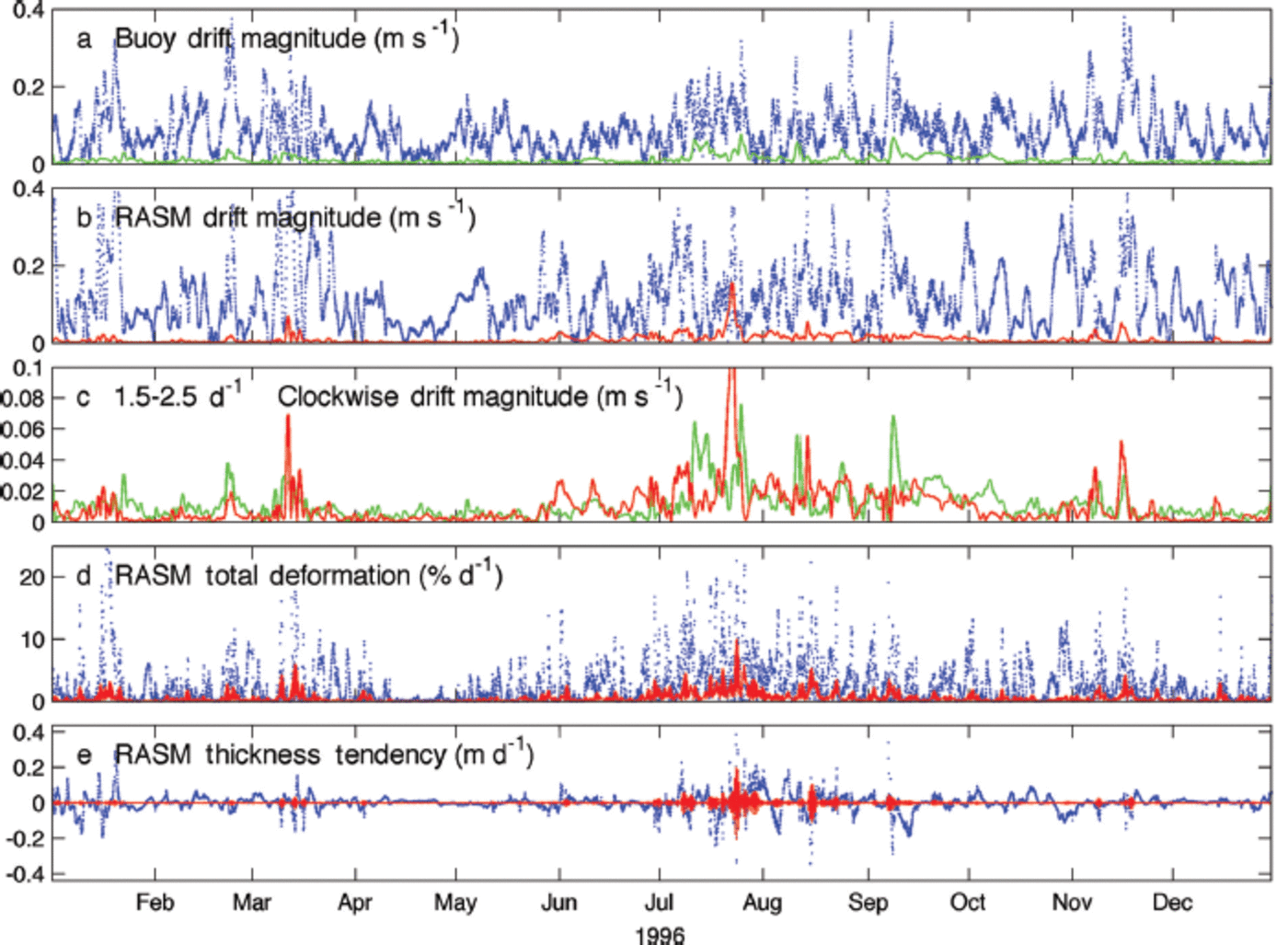
A further advantage of rotary wavelet analysis is that it provides a measure of the relative agreement of both power and periodicity of two signals at a specific point in time. This is achieved via the wavelet coherence squared statistic (R ²), which can be thought of as a frequency space analogue to correlation in time. However, the most important property of the R ² statistic is that relatively small differences between time series can result in poor coherence squared values. This is further explained in Appendix B, but the key point here is that statistically significant R ² values exceeding 0.9 indicate very close agreement between a model and observations, in this case for sea-ice drift magnitude at a given frequency and rotation sense. There is strong coherence of ice motion between RASMe1 and IABP 9364 near or at the clockwise half-day period during summer, when inertial oscillations were most pronounced (Fig. 6e). However, for the remainder of the year, there is less agreement except in the case of rare, statistically significant inertial oscillation events. A similar result exists in the wavelet comparison of IABP 9365 with RASMe1 (not shown). However, that comparison is less straightforward because IABP 9365 was deployed after much of the 1996 summer had passed.

The corresponding time series illustrate the observed (Fig. 7a) and modeled (Fig. 7b) broadband (all-frequency) drift corresponding to IABP 9364. The corresponding inertial drift magnitude is isolated using a clockwise 1.5-2.5 d ^-1 rotary filter, shown in green for IABP 9364 (Fig. 7a), and in red for the collocated RASMe1 time series (Fig. 7b). Methods used to prepare Figure 7 are described in Appendix B. When interpreting the direct comparison between inertial oscillation magnitude in the model and that of buoy IABP 9364 (Fig. 7c), it is important to take into account that RASM is fully coupled. Therefore the precise timing and strength of inertial oscillations will rarely line up exactly, because RASM is subject to internal variability in the same way as global fully coupled models are, except here this variability is only regional. Still, in some cases the timing of modeled and observed extreme events closely matches, especially where weather systems passing over the ice are driven by longwave atmospheric circulation, to which RASM is closely constrained by boundary conditions.

One should expect similar seasonality and non-stationary high-frequency sea-ice drift in the model to that in the observations, which we submit is the case when assessing Figures 5-7 together. The key outcome of these results is that overall RASMe1 and IABP 9364 inertial sea-ice drift speeds are comparable within the bounds of differences stemming from seasonal variability. This is also evident in the close agreement between the major peaks in modeled and observed rotary spectral drift (Fig. 5, within the -1.5 to +1.5 d ^-1 frequency range). Although inertial oscillations typically constitute a small fraction of total speed in both the modeled and buoy drift (Fig. 7), they contribute more substantially to total deformation and thickness in RASM. This can be seen by comparing the red trace with the blue time series in Figure 7d and e where total deformation and thickness tendency includes both dynamics and thermodynamics. It is evident that for the most part, inertial oscillations contribute background noise to the sea-ice drift solution, interspersed with non-stationary pulses significant in the complete deformation signal. These pulses predominantly occur during summer.

Seasonality and Spatial Distribution of Inertial Oscillations in RASMe1 During 1996

While high-frequency drift and deformation is statistically dominated by small values, there are comparatively rare yet extreme inertial oscillations and associated sea-ice fracture in the modeled and observed drift records presented in the previous section. Such extreme events are evident at the 2 d ^{- 1} wavelet power (Fig. 7). To further analyze these statistical characteristics in the model, we filtered clockwise 1.8-2.1 d ^{- 1} drift and deformation from hourly RASMe1 output. These filtered data were then used to construct probability density curves for January-March and July-September 1996 over the Arctic Ocean. The probability density curves have been divided into four categories based upon the mean thickness of the drifting ice: ˂ 1, 1-2, 2-3 and ˃3 m (Fig. 8). Mean thickness, as defined here, is the thickness of each sea-ice category in CICE, weighted by their individual concentration. It is therefore a measure of both the mass and compactness of the ice cover. The derived distributions more closely resemble a log-normal distribution in summer than in winter, pointing to extreme values being most prevalent in summer. This is, to our knowledge, the first presentation of a basin-wide direct statistic of the sea-ice inertial oscillation speed for a coupled model.

Fig. 8.

RASMe1 normalized probability density of (a) 1.8-2.1 d-¹ clockwise inertial drift and (b) corresponding divergence magnitude for model gridcells in the central Arctic analysis region. Individual histograms are filtered to include only the mean gridcell thickness and 3 month period as denoted in the legend (January-March and July-September). Hourly samples with sea-ice concentration ˂15% are excluded. N indicates the total number of hourly samples used to construct each histogram after applying the mask, using 2.5 x 10^-3 ms-¹ and 2.5 x 10^-8ms-¹ bin sizes for drift and deformation, respectively.

For the RASMe1 case-study year, inertial oscillation speed and associated deformation are negligible during January-March relative to July-September, even in their extreme values (Fig. 8). They indicate that between winter and summer the pattern shifts toward much stronger oscillations across the central Arctic. Perhaps more importantly, the results from RASM also indicate that the summer shift observed in this case study is not solely attributable to the state of the pack, as demonstrated by the closely clustered curves of each thickness division (Fig. 8). This is evidence that the most significant reason for seasonal differences between summer and winter inertial oscillations is storm activity, rather than factors associated with sea-ice thickness or concentration, as indicated by seasonal differences in surface circulation (Fig. 3). We concede that the RASMe1 realization possesses slightly heightened seasonality in inertial oscillation relative to the buoy record, as indicated by the wavelet analysis (Fig. 6). However, this does not detract from the important point that a change in cyclonic activity, including frequency of occurrence and seasonal shifts, could equally contribute to change in 21st-century summer inertial oscillations as could Arctic sea-ice thickness decline. The relationship between climatic changes in sea-ice thickness and storm activity is not easily separated in the complex adaptive Arctic system.

To further demonstrate the seasonal shift in high-frequency drift and divergence magnitude, we analyze spatial distribution of the median inertial oscillation speed for January-March and July-September (Fig. 9), and corresponding root-mean-square (rms) divergence calculated from the clockwise signal (Fig. 10). Note that rms divergence is the most appropriate divergence statistic in this case, since the high-frequency divergence signal oscillates around zero. These have been calculated using methods described in Appendix B and are, to our knowledge, the first direct basin-wide statistics of inertial speed and deformation shown for a coupled model. Overlaid on these maps are mean sea-level pressure (Fig. 9) and mean thickness (Fig. 10). Comparing these overlaid statistics between Figures 8 and 10, a thickness bias clearly exists in inertial oscillation and deformation magnitude, but it is also evident that the magnitude of inertial oscillations is influenced by the location of Arctic cyclonic activity. In particular, rms divergence during July-September (Fig. 10) shows strong deformation in ice ˂2m thick in the Canada Basin, but comparatively quiescent conditions across much of the Amundsen and Nansen basins with ice of similar thickness. A difference between the two regions is that a seasonal depression extends over the areas with greater inertial motion in sea ice, seen in the surface pressure for July-September (Fig. 9).

Fig. 9.

(a) January-March and (b) July-September 1996 median clockwise 1.8-2.1 m d ^{- 1} sea-ice drift magnitude. This indicates the inertial speed on a logarithmic color scale for RASMe1 within the central Arctic analysis domain defined in Figure 1 . Black contours indicate the corresponding surface air pressure at 1hPa spacing (solid ˃1015 hPa; bold 1015 hPa; dashed ˂1015hPa). Areas where the sea-ice concentration is ˂15% at any time in the analysis period are excluded. Corresponding sea-ice thickness and divergence are provided in Figure 10. These spatial medians correspond to the histogram of hourly instantaneous values in Figure 8a.

Fig. 10.

(a) January-March and (b) July-September 1996 rms divergence (s^-1) for clockwise 1.8-2.1 d ^{- 1} sea-ice drift. Black contours indicate the mean sea-ice thickness at 1m spacing (solid ˃2m; bold 2m; dashed 1m). Areas where the sea-ice concentration is ˂15% at any time in the analysis period are excluded. Corresponding sea-ice inertial speed and surface air pressure are provided in Figure 9. The rms statistic shown here may be compared with the divergence magnitude histogram in Figure 8b.

These results suggest a more subtle connection between sea-ice thickness and inertial oscillations in the pack than may have previously been understood. Cyclones over the ice-ocean boundary layer result in surface divergence in their wake, and associated Ekman transport and pumping, which is indicated by sea-ice inertial oscillations. These dynamics themselves are associated with near-surface mixing and may result in changes in sea-ice thickness stemming from changes in the oceanic heat flux. Therefore, the strength and prevalence of low-pressure systems traversing the central Arctic in summer needs to be considered when investigating climatic changes in ice-ocean Ekman transport in the Arctic as part of the same coupled system. This is the reason for the strong seasonal shift in inertial speed and deformation (Fig. 8), irrespective of the mean sea-ice thickness sampled. This is especially relevant in light of recent extreme events, such as the ‘Great Arctic Cyclone’, which resulted in the 2012 record September minimum sea-ice extent in the satellite era (Reference Simmonds and RudevaSimmonds and Rudeva, 2012).

Applying Rasm Coupling Methods in the Community Earth System Model

To place the RASM case study in context and to demonstrate the consequence of frequent atmosphere-ice-ocean coupling in a global Earth System Model, we have applied the RASM ice-ocean coupling configuration to CESM. The standard version of CESM uses a 30min ‘fast’ coupler time step to exchange fluxes between the atmosphere, land and sea-ice models, and a ‘slow’ coupler time step to exchange the ocean model daily fluxes with other components via CPL7. In this configuration the ocean model completes twenty-four 1 hour oceanic time steps within each coupler period. A natural consequence of this configuration is that even though the ocean model’s internal time step and physics sufficiently resolve Ekman mass transport, the coupling paradigm does not. In this configuration the Nyquist coupling frequency is 0.5 d^-1which exceeds all inertial frequencies within sea-ice zones. To demonstrate the impact this has on ice-ocean Ekman transport, we completed two CESM integrations, one using CPL7 and another using CPL7x, the latter with the ocean model in the ‘fast’ 30min coupling mode. This also required the modification of ocean model time step to allow 17 steps per 30 min to ensure a non-diffusive ratio of leapfrog to forward time steps in POP. All other aspects of the ocean configuration conform to the public release of CESM Version 1.1, and a summary of the CESM discretization used in this test is provided in Table 2 . In this study, the CESM sea-ice model configuration uses the same Reference Brunke, Zhou, Zeng and AndreasBrunke and others (2006) variable sea-ice roughness length additions as described for RASM in Appendix A.

Table 2.

Configuration of the Community Earth System Model used in this paper, including changes made to incorporate high-frequency oceanic coupling in italics

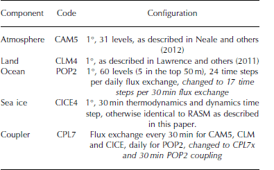
A comparison between the two coupling methods was conducted by initializing CESM with pre-industrial initial conditions, spun up over many centuries, then integrating the model forward for one simulated year, with and without the RASM coupling changes. Even though this spawns two different realizations over which climate model comparisons would normally be invalid, the high-frequency nature of the inertial signal allows meaningful comparison between the two short simulations for the physics of interest.

The change in CESM coupling has a substantial impact on the high-frequency component of the ice motion in the Arctic Ocean (Fig. 11). Whereas the standard configuration of CESM possesses little, if any, inertial signal (at -2 d^-1) in sea-ice drift (Fig. 11, blue line), the configuration using the CPL7x coupler with 30 min oceanic flux exchange does exhibit the inertial signal (Fig. 1 1, red line). The significance of this difference is not that a relatively minor long-term drift signal has been added to CESM’s sea-ice solution. Rather, the red peaks at -2 d ^{- 1} (Fig. 11) represent the inclusion of a process previously neglected: ice-ocean Ekman layer dynamics, including transient transport and pumping. This has important implications for oceanic mixing under sea ice during the passage of storms. A minor point to note is that small anticlockwise peaks are also added to the drift signal at +2d^-1indicating that internal sea-ice stress is smearing inertial loops into ellipses, as discussed earlier. We suggest that this is an artifact of lower resolution used in CESM, as compared to RASM.

Fig. 11.

Rotary power spectral density of sea-ice drift for a 1 year pre-industrial simulation of CESM with (red) and without (blue) high-frequency ocean coupling (CPL7x 30 min ocean coupling and CPL7 daily ocean coupling respectively). The locations of the model gridpoints for which the spectra were calculated in (a) and (b) are indicated in Figure 1.

Modifying the coupling in CESM has a large impact on the median inertial sea-ice speed in both the Arctic (Fig. 12) and Antarctic (Fig. 13). These figures were generated by rotary filtering CESM sea-ice velocity at each model gridpoint within ±0.1 d-¹ of the local inertial frequency wherever the mean sea-ice concentration exceeded 15% for each 3 month period shown. In both the Arctic and Antarctic, but particularly the Southern Ocean, improved modeling of ice-ocean Ekman transport can result in an order-of-magnitude increase in the median seasonal magnitude of inertial oscillations across vast tracts of the pack (Fig. 12 and 13). Note that the vertical ocean resolution of CESM is considerably less than in RASM, and one may expect an even stronger response in CESM if the number of vertical POP layers is increased close to the surface. The importance of the relative roles of sea-ice strength and storm location, frequency and intensity in determining the magnitude of ice-ocean Ekman transport remains to be determined and is a question we intend to pursue using RASM and CESM in a follow-on study.

Fig. 12.

Arctic median inertial sea-ice speed for a 1 year pre-industrial simulation of CESM without and with high-frequency ocean coupling. (a, b) A standard CESM case with daily ocean coupler steps in combination with 30 min coupler steps for the atmosphere, land and sea-ice components during (a) January-March and (b) July-September. (c, d) The equivalent values for 30 min coupler steps for all of the atmosphere, land, sea ice and ocean for the same periods: (c) January-March and (d) July-September. The color scale is logarithmic and identical to that in Figure 9.

Fig. 13.

Same as Figure 12, but for the Antarctic and showing anticlockwise inertial speed.

Discussion

Perhaps the most important outcome of this investigation is evidence of the significant impact of the coupling time step used in Earth System Models. This point is seldom discussed in the literature, but is important near the poles, where the inertial oscillation period is smallest. By comparing CESM coupling methods with a regionally constrained counterpart (RASM), we have addressed a question that has not been adequately answered in the literature.

Previously it has been suggested that coupled ice-ocean models that do not embed sea ice in the ocean may not adequately simulate inertial oscillations (Reference Hibler, Roberts, Heil, Proshutinsky, Simmons and LovickHibler and others, 2006). By ‘embed sea ice’, we mean using an ocean coordinate system that allows Archimedes’ principle to apply so that sea ice ‘floats’ in the ocean model, with the resultant pressure force affecting the ocean’s barotropic mode (Reference Hibler, Roberts, Heil, Proshutinsky, Simmons and LovickHibler and others, 2006). Within the versions of RASM and CESM used in this study, sea ice is ‘levitated’, meaning that ice-ocean dynamical coupling is driven purely by their interfacial stresses, and the ocean is not influenced by sea-ice buoyancy. We have demonstrated that this levitated coupling mechanism, while not physically perfect, can model inertial oscillations of similar magnitude to those observed in the pack, as indicated by wavelet coherence. This is not to say that the sea-ice embedding would not improve ice-ocean boundary layer physics. Rather, a z* coordinate system, which is a way of embedding sea ice in the ocean (Reference Campin, Marshall and FerreiraCampin and others, 2008), is probably more important for improving the barotropic mode for oceanic tides, a component not addressed in this study. Instead, we suggest that a coupling configuration that tightly synchronizes the ice-ocean, atmosphere-ice and atmosphere-ocean interfacial stress terms is the most important model mechanism required to simulate high-frequency sea-ice mechanics. This addresses our main aims stated in the introduction, and lays open the use of CESM for investigations to understand the climatic influence of storm passage over sea ice in both the Arctic and Southern Ocean.

Both RASM and CESM use five sea-ice thickness categories to approximate sea-ice strength based upon the work of Reference RothrockRothrock (1975). This approach is more sophisticated than the two-category compressive strength approximation of Reference Hibler, Heil and LytleHibler (1979) used in several present-day global models (IPCC, 2013), and produces a markedly different result in high-resolution models (Reference Maslowski and LipscombMaslowski and Lipscomb, 2003). With this in mind, the RASMe1 case study indicates that both the state of the pack and cyclonic activity are important factors that need to be assessed together in understanding inertial motion in sea ice. Therefore it is important that inertial motion is not considered a metric for just thickness and concentration changes, owing to dependence of the strength of Ekman transport on storm activity. For this reason we suggest that it is premature to attribute climatic changes in Arctic inertial oscillations to thickness changes alone. However, there is clear observational evidence that near-inertial waves in the Arctic Ocean are larger and more prevalent in less concentrated sea ice (Fer, 2014; Reference Maraun and KurthsMartini and others, 2014), which corresponds to thinner ice using our mean thickness statistic.

Both RASM and CESM use five sea-ice thickness categories to approximate sea-ice strength based upon the work of Reference RothrockRothrock (1975). This approach is more sophisticated than the two-category compressive strength approximation of Reference Hibler, Heil and LytleHibler (1979) used in several present-day global models (IPCC, 2013), and produces a markedly different result in high-resolution models (Reference Maslowski and LipscombMaslowski and Lipscomb, 2003). With this in mind, the RASMe1 case study indicates that both the state of the pack and cyclonic activity are important factors that need to be assessed together in understanding inertial motion in sea ice. Therefore it is important that inertial motion is not considered a metric for just thickness and concentration changes, owing to dependence of the strength of Ekman transport on storm activity. For this reason we suggest that it is premature to attribute climatic changes in Arctic inertial oscillations to thickness changes alone. However, there is clear observational evidence that near-inertial waves in the Arctic Ocean are larger and more prevalent in less concentrated sea ice (Fer, 2014; Reference Maraun and KurthsMartini and others, 2014), which corresponds to thinner ice using our mean thickness statistic.

Aside from the particular focus of this research on inertial oscillations, we have demonstrated the utility of a coupled regional model as a tool for model evaluation. We reemphasize that direct comparisons between global coupled models and observations typically require long data records, but for the physics of interest, few buoy records last more than 3 years, often much less, and can be disparately located in the Arctic at any point in time. We have employed a method of constructing the required modeling infrastructure in an Arctic regional model, evaluating it against daily observations in a fully coupled framework, and then applied it to a global coupled model to understand the global significance. In so doing, we have confidence that ice-ocean inertial oscillations and processes associated with them are realistic in CESM when using the coupler improvements engineered in RASM.

Conclusion

The main aim of this work is to demonstrate the impact of the temporal resolution of flux exchanges on integrated ice-ocean dynamics in Earth System Models. By combining Ekman theory with rotary signal-processing techniques, we have used high-frequency sea-ice velocity as a proxy for the strength of Ekman transport, and thereby of high-frequency ice-ocean dynamics important for the exchange of heat and momentum between polar oceans and the atmosphere. Whereas previous studies on this topic have focused primarily on the impact of ice-ocean Ekman transport on sea-ice drift and deformation, we have framed our investigation in terms of the broader question of whether or not sufficient mixing is being stimulated in the ice-ocean system during the passage of storms. Results in RASM agree with previous studies (e.g. Reference Heil and HiblerHeil and Hibler, 2002) suggesting a significant contribution of high-frequency inertial oscillations to total deformation and thickness change in sea ice (Fig. 7).

By applying a rotary wavelet filter to RASM and CESM sea-ice velocities, we have calculated the hourly inertial speed of three model realizations and provided statistics that address missing physics in some present-day Earth system models related to oceanic mixing in response to passage of storms. By resolving ice-ocean inertia in CESM, there is an order-of-magnitude increase in the median speed of inertial oscillations across large areas of the Southern Ocean pack in winter and summer. The speed increase is more modest in Northern Hemisphere sea ice, but still remains elevated relative to daily oceanic coupling in CESM. This result indicates a need to analyze sea-ice inertial speed, storm tracks and oceanic mixing together in a fully coupled system, in which sea-ice thickness is but one variable subject to coupled feedbacks. To our knowledge, this is the first time the global distribution of rotational-sense sea-ice motion has been calculated and presented in this way for an Earth System Model.