1. INTRODUCTION
Experiments such as LIGHT (Schollmeier et al., Reference Schollmeier, Becker, Geissel, Flippo, Blaević, Gaillard, Gautier, Grüner, Harres, Kimmel, Nürnberg, Rambo, Schramm, Schreiber, Schütrumpf, Schwarz, Tahir, Atherton, Habs, Hegelich and Roth2008; Bagnoud et al., Reference Bagnoud, Aurand, Blazevic, Borneis, Bruske, Ecker, Eisenbarth, Fils, Frank, Gaul, Goette, Haefner, Hahn, Harres, Heuck, Hochhaus, Hoffmann, Javorková, Kluge, Kuehl, Kunzer, Kreutz, Merz-Mantwill, Neumayer, Onkels, Reemts, Rosmej, Roth, Stoehlker, Tauschwitz, Zielbauer, Zimmer and Witte2010; Busold et al., Reference Busold, Schumacher, Deppert, Brabetz, Frydrych, Kroll, Joost, Al-Omari, Blažević, Zielbauer, Hofmann, Bagnoud, Cowan and Roth2013; Reference Busold, Almomani, Bagnoud, Barth, Bedacht, Blažević, Boine-Frankenheim, Brabetz, Burris-Mog, Cowan, Deppert, Droba, Eickhoff, Eisenbarth, Harres, Hoffmeister, Hofmann, Jaeckel, Jaeger, Joost, Kraft, Kroll, Kaluza, Kester, Lecz, Merz, Nürnberg, Al-Omari, Orzhekhovskaya, Paulus, Polz, Ratzinger, Roth, Schaumann, Schmidt, Schramm, Schreiber, Schumacher, Stoehlker, Tauschwitz, Vinzenz, Wagner, Yaramyshev and Zielbauer2014a; Reference Busold, Schumacher, Deppert, Brabetz, Kroll, Blažević, Bagnoud and Roth2014b) have proven the possibility of producing and manipulating intense ion beams with the use of high-power lasers. The acceleration process occurring in these experiments is the target normal sheath acceleration (TNSA) (Snavely et al., Reference Snavely, Key, Hatchett, Cowan, Roth, Phillips, Stoyer, Henry, Sangster, Singh, Wilks, MacKinnon, Offenberger, Pennington, Yasuike, Langdon, Lasinski, Johnson, Perry and Campbell2000; Wilks et al., Reference Wilks, Langdon, Cowan, Roth, Singh, Hatchett, Key, Pennington, MacKinnon and Snavely2001; Mora, Reference Mora2006; Ceccotti et al., Reference Ceccotti, Lévy, Réau, Popescu, Monot, Lefebvre and Martin2008; Passoni et al., Reference Passoni, Bertagna and Zani2010; Lécz et al., Reference Lécz, Boine-Frankenheim and Kornilov2013). Light ion beams (e.g., protons) are accelerated to energies in the range of 3–50 MeV with an exponentially density distribution. Due to the advance in laser technology and target production, a new laser ion acceleration mechanism has become of interest: The radiation pressure acceleration (RPA). As simulation show (Esirkepov et al., Reference Esirkepov, Borghesi, Bulanov, Mourou and Tajima2004; Macchi et al., Reference Macchi, Cattani, Liseykina and Cornolti2005; Reference Macchi, Veghini and Pegoraro2009; Reference Macchi, Veghini, Liseykina and Pegoraro2010; Robinson et al., Reference Robinson, Zepf, Kar, Evans and Bellei2008; Rykovanov et al., Reference Rykovanov, Schreiber, Meyer-ter Vehn, Bellei, Henig, Wu and Geissler2008; Shoucri Reference Shoucri2012; Shoucri et al., Reference Shoucri, Lavocat-Dubuis, Matte and Vidal2011; Reference Shoucri, Matte and Vidal2013; Reference Shoucri, Matte and Vidal2014; Henig et al., Reference Henig, Steinke, Schnürer, Sokollik, Hörlein, Kiefer, Jung, Schreiber, Hegelich, Yan, Meyer-Ter-Vehn, Tajima, Nickles, Sandner and Habs2009; Schlegel et al., Reference Schlegel, Naumova, Tikhonchuk, Labaune, Sokolov and Mourou2009; Kar et al., Reference Kar, Kakolee, Qiao, Macchi, Cerchez, Doria, Geissler, Mckenna, Neely, Osterholz, Prasad, Quinn, Ramakrishna, Sarri, Willi, Yuan, Zepf and Borghesi2012; Korzhimanov et al., Reference Korzhimanov, Efimenko, Golubev and Kim2012), this mechanism produces heavy-ion (e.g., Gold, Titanium, Carbon etc.) beams with intensities orders of magnitude larger than in the case of the TNSA. Typically, narrow band energies in the range of GeV are observed, wherein the ions show nearly solid body densities. This opens a wide field of new applications, such as medical applications (tumor therapy), neutron sources, diagnostic tools, etc. (Roth et al., Reference Roth, Cowan, Key, Hatchett, Brown, Fountain, Johnson, Pennington, Snavely, Wilks, Yasuike, Ruhl, Pegoraro, Bulanov, Campbell, Perry and Powell2001; Reference Roth, Jung, Falk, Guler, Deppert, Devlin, Favalli, Fernandez, Gautier, Geissel, Haight, Hamilton, Hegelich, Johnson, Merrill, Schaumann, Schoenberg, Schollmeier, Shimada, Taddeucci, Tybo, Wagner, Wender, Wilde and Wurden2013). Therefore many upcoming experiments aim at this acceleration mechanism. The first experimental success was shown in (Aurand et al., Reference Aurand, Kuschel, Jäckel, Rödel, Zhao, Herzer, Paz, Bierbach, Polz, Elkin, Paulus, Karmakar, Gibbon, Kuehl and Kaluza2013; Kim et al., Reference Kim, Pae, Kim, Kim, Lee, Choi, Singhal, Sung, Lee, Lee, Nickles and Nam2014). To obtain the RPA mechanism, target thicknesses in the range of d = 10–100 nm and particle densities of n ≈ 1000n c as well as circular polarized lasers with intensities of I 0 = 5 × 10²⁰−5 × 10²² W cm−2 and pulse lengths of τ = 20−150 fs, are required. The circular polarization of the laser prevents electron heating effects, usually obtained in connection with the TNSA mechanism. This work faces on the optimization of the RPA beam quality in dependence of the laser and target parameters. In the first stage, a relativistic two fluid model of the laser plasma interaction is derived. From this analytical model, two important perceptions are obtained: First, an approximation to the maximum achievable kinetic energy is derived. Within this, a termination criterion for the RPA mechanism is achieved, above which the acceleration process collapses. In addition to that, a minimum requirement for the target thickness is observed. The second part of this paper faces on the question of the optimization of the RPA. An analytical prediction is supported by a one-dimensional (1D) Particle in Cell (PIC) simulation, to work out the optimum working point for the acceleration process.
2. THE TWO FLUID MODEL FOR PLASMA
The target is modeled as a relativistic two-fluid mixture, consisting of ions (i) of mass m i and charge number Z and the corresponding electrons (e) (mass m e, charge −e). Both species are assumed to be ideal gases with densities n i and n e, respectively (Dendy, Reference Dendy1990; Kegel, Reference Kegel1998; Boyd et al., Reference Boyd, Sanderson and Zita2006). These assumptions could be justified by claiming that the pre-pulse of the laser has ionized the target by multiple-stage ionization, just before the main acceleration takes place. The thermal drift of the plasma is of minor importance on the time scale of the laser pulse.
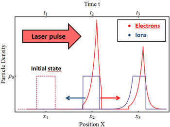
Figure 1 shows the principle course of a radiation pressure acceleration: The incident laser pulse compresses the electron gas due to the radiation pressure, while the much more inert heavy ions are unaffected. The resulting charge separation leads to a polarization field which causes an electron flow into the positive x-direction and an ion flow into the opposite direction. By that, the amount of particles in the plasma center is continuously reduced. The central part of the ions is accelerated in this polarization field and thereby dragged by the electrons. Since the plasma is overdense initially, the laser wave is evanescent in the plasma. If the initial plasma has a thickness d and a refractive index N, the evanescent signal of the laser wave propagates through the plasma with a velocity c′ = c/N and is partly reflected at the rear surface of the plasma. This back and forth propagation of the signal takes the time τEM = 2d/c′. Usually the laser pulse length is much longer than this propagation time: τL ≫ τEM. Therefore an evanescent equilibrium state forms in the plasma slab, on a time scale at which the laser amplitude undergoes no significant change. A measure for that would be the number N R:
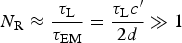 $$N_{\rm R} \approx \displaystyle{{{\rm \tau} _{\rm L}} \over {{\rm \tau} _{{\rm EM}}}} = \displaystyle{{{\rm \tau} _{\rm L} c^{\prime}} \over {2d}} \gg 1 $$
In addition to that, the electron relaxation time  ${\rm \tau} _{{\rm relax}}^{\rm e} \propto 1/{\rm \omega} _{{\rm pe}} $ is much smaller than the propagation time:
 $${\rm \tau} _{{\rm relax}}^{\rm e} \ll {\rm \tau} _{{\rm EM}}$$
Sketch of the RPA mechanism: The laser compresses the electron gas (red). The resulting polarization field drags the ions (blue).

Under these conditions, a quasi-static equilibrium state in the plasma slab builds up, which only slowly varies on the time scale of the laser.
3. DERIVATION OF THE MODEL
The easiest way to deal with this model is to transform the equations into a moving reference frame.
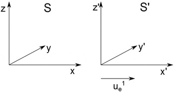
Consider a system S′ which moves with velocity  $u_{\rm e}^{\rm 1} $ in the positive x-direction (see Fig. 2). Here we introduced the four-vector style, where
 $U_{{\rm e,i}}^{\rm \alpha} = {\rm \gamma} _{{\rm e,i}} (c,\vec u_{{\rm e,i}} )^{\rm T} $ is the electrons (e) or ions (i) four-velocity. The notation then reads:
 $u_{{\rm e,i}}^0 = {\rm \gamma} _{{\rm e,i}} c$,
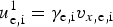 $u_{{\rm e,i}}^{\rm 1} = {\rm \gamma} _{{\rm e,i}} v_{x{\rm, e,i}} $,
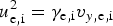 $u_{{\rm e,i}}^{\rm 2} = {\rm \gamma} _{{\rm e,i}} v_{y{\rm, e,i}} $,
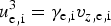 $u_{{\rm e,i}}^{\rm 3} = {\rm \gamma} _{{\rm e,i}} v_{z{\rm, e,i}} $. Furthermore, we will label a quantity with a prime if it is treated in the co-moving reference frame and without, if it is determined in the laboratory frame S. This means, that S′ is a system, perfectly co-moving with the electrons. Even if
 $u_{\rm e}^{\rm 1} (x,t)$ is a function of space and time (x,t), there will always be a system, where the electron velocity vanishes locally. As shown in literature (Rebhan, Reference Rebhan2012), this leads to a geodesic equation for the metrical tensor and the Lorentz-transformation does not remain linearFootnote 1. But as justified in Mulser and Bauer (Reference Mulser and Bauer2010), the deviations from the linear Lorentz-transformation (with a constant velocity, v) are of higher order and small and can thus be neglected. A proof of this assumption is given in the Appendix. For the moment we perform a linear Lorentz-transformation, keeping in mind that this assumption may only be valid locallyFootnote 2. This Ansatz is typically used in relativistic hydrodynamics (Fliessbach, Reference Fliessbach2012; Rebhan, Reference Rebhan2012). From the conservation of angular momentum it follows ∑kLk = L e + L i = 0, since the angular momentum is zero initially. Electrons and ions both rotate with the Doppler shifted laser frequency ω′. Since
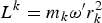 $L^k = m_k {\rm \omega} ^{\prime}r_k^{\rm 2} $, this reads (k = e, i):
 $r^{\rm i} /r^{\rm e} = \sqrt {m_{\rm e} /m_{\rm i}} $. We note that since S′ moves into the x-direction, the perpendicular lengths do not change:
 $r_k^{\rm ^{\prime}} = r_k $. Moreover the azimuthal velocity is given by:
 $\vec u_{k \bot} ^{\,\prime} = {\rm \omega} ^{\prime}r_k $. Hence, the ratio of the azimuthal velocities is given by:
 $\vec u_{{\rm i} \bot}^{\,\prime}/\vec u_{{\rm e} \bot} ^{\,\prime} = \sqrt {m_{\rm e} /m_{\rm i}} \ll 1$. Therefore the ions contribution to the azimuthal current can be neglected (due to the larger mass of the ions). This assumption is useful, since it decouples the ions from the perpendicular part of the Maxwell equations. The relativistic equations of motion for the electrons then read:
 $${{\partial}} _{{t}^{\prime}} n_{\rm e}^{\prime} = 0$$
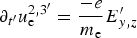 $${\partial}_{t^{\prime}} u_{\rm e}^{2,3^{\prime}} = \displaystyle{{ - e} \over {m_{\rm e}}} E_{y,z} ^{\prime} $$
 $${\partial}_{t^{\prime}t^{\prime}} E_{y,z} ^{\prime} - c^2 {\partial}_{x^{\prime}x^{\prime}} E_{y,z} ^{\prime} = \displaystyle{{en_{\rm e} ^{\prime}} \over {{\rm \varepsilon} _0}} {\partial}_{t^{\prime}} u_{\rm e}^{2,3^{\prime}} $$
In the co-moving system S′ the particle concentration  $n_{\rm e} ^{\prime} =$
 $n_{\rm e} ^{\prime}(x^{\prime})$ is a function of x′ onlyFootnote 3. Putting both systems of equations together yields:
 $${\partial}_{t^{\prime}t^{\prime}} E_{y,z} ^{\prime} - c^2 {\partial} _{x^{\prime}x^{\prime}} E_{y,z} ^{\prime} = - \displaystyle{{e^2 n_{\rm e} ^{\prime}} \over {{\rm \varepsilon} _0 m_{\rm e}}} E_{y,z} ^{\prime}$$
Standard configuration of a laboratory system S and a moving frame S′, which propagates in the positive x-direction.

This is a Klein–Gordon equation (Whitham, Reference Whitham1974) for the electrical field components perpendicular to the propagation direction. A similar result can be obtained in the laboratory frame by a perturbation theory, like it is shown in many textbooks. It should be noted, that the electromagnetic (EM) field components perpendicular to the propagation direction are solenoidal at the beginning and remain so over the entire time. In the following sections, we will derive some qualitative results from Eq. (6) and compare them with PIC simulations.
4. APPROXIMATION FOR THE VELOCITY LIMIT
If we chose a monochromatic wave Ansatz  $E^{\prime}_{y,z} \propto \exp (i(w^{\prime}t^{\prime} - $
 $ k^{\prime}x^{\prime}))$ and for the moment treat
 $n_{\rm e} ^{\prime}$ as a constant, we obtain the dispersion relation:
 $${\rm \omega}^{\prime 2} = k^{\prime 2} c^2 + {\rm \omega} _{{\rm pe}}^{\rm 2}$$
where  ${\rm \omega} _{{\rm pe}}^{\rm 2} = n_{\rm e} e^2 /{\rm \varepsilon} _0 m_{\rm e} $ is the plasma frequency of the electrons. In the region where
 $n_{\rm e} ^{\prime}(x^{\prime}) \gt 0$ holds, this equation means, that
 ${\rm \omega}^{\prime} \ge {\rm \omega} _{\rm pe} \;\forall k \in {\rm \opf R}$. In other words, if the laser frequency ω′ is lower than the electron plasmafrequency ωpe, there is no propagating wave possible in the plasma. From that follows, that
 $k^{\prime} \in {\rm \opf C}\forall {\rm \omega}^{\prime} \lt {\rm \omega} _{{\rm pe}} $. This means, that the EM wave is evanescent in the plasma. A Lorentz-transformation with respect to
 $v = - u_{\rm e}^{\rm 1} $ re-transforms Eq. (7) into the laboratory frame S (see Fig. 2). There it holds:
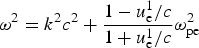 $${\rm \omega} ^2 = k^2 c^2 + \displaystyle{{1 - u_{\rm e}^{\rm 1} /c} \over {1 + u_{\rm e}^1 /c}}{\rm \omega} _{{\rm pe}}^{\rm 2}$$
From rearranging this formula one obtains:
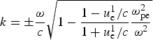 $$k = \pm \displaystyle{{\rm \omega} \over c}\sqrt {1 - \displaystyle{{1 - u_{\rm e}^{\rm 1} /c} \over {1 + u_{\rm e}^{\rm 1} /c}}\displaystyle{{{\rm \omega} _{{\rm pe}}^2} \over {{\rm \omega} ^2}}}$$
If the radicand of the square root gets greater than zero, k is the element of the reals and therefore the EM field transforms into a propagating wave. This effect is called Doppler transparency. For the plasma frequency in the rest-frame S,  ${\rm \omega} _{{\rm pe}}^{\rm 2} = e^2 n_{\rm e} /{\rm \gamma} _{\rm e} {\rm \varepsilon} _0 m_{\rm e} $ holds, with
 ${\rm \gamma} _{\rm e}^{\rm 2} = 1 + {\rm \alpha} _{\rm e}^{\rm 2} $ being the electrons relativistic factor. Since αe = eE 0/m eωc it depends on the laser amplitudeFootnote 4. By that the electron plasma frequency is decreased in the presence of high laser amplitudes. This clearly means, that the electron mass increases while oscillating in the laser field and thus the oscillation frequency decreases. In the region where n e < n c holds, the evanescent wave turns into a propagating wave again. If an adequate fraction of the laser wave penetrates the target, the RPA is disturbed, as explained in the previous section. As stated earlier, it is difficult to gain the exact distribution
 $n_{\rm e} ^{\prime}$ for the electrons, but we can change the geometry of the problem without loss of generality. Assume the electrons have a step-like distribution of thickness d, that is:
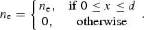 $$n_{\rm e} = \left\{\matrix{ {n_{\rm e},} & {{\rm if}\;0 \le x \le d} \cr {0,} & {{\rm otherwise}} \cr} \right..$$
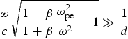
The continuity equation then transforms into: n e(t)d(t) = n e0d 0, where the zero denotes the initial values. If we introduce a compression factor ϰ e = n e(t)/n e0, this reads: d(t) = d 0/ϰ e. The penetration-depth of the EM wave is given by δe = 1/k, with k from Eq. (9). If the penetration-depth becomes larger than the effective thickness, the laser penetrates the plasma: δ/d ≫ 1. Rearranging Eq. (9) and keeping in mind that , we get:
 $$\displaystyle{{\rm \omega} \over c}\sqrt {\displaystyle{{1 - {\rm \beta}} \over {1 + {\rm \beta}}} \displaystyle{{{\rm \omega} _{{\rm pe}}^{\rm 2}} \over {{\rm \omega} ^2}} - 1} \gg \displaystyle{1 \over d} $$
Solving this equation for β leads to:
 $${\rm \beta} _{{\rm max}}^{\rm e} \le \displaystyle{{1 - \left( {1 + (c^2 \varkappa _{\rm e}^{\rm 2} /{\rm \omega} ^2 d_0^2 )} \right)({\rm \omega} ^2 /{\rm \omega} _{{\rm pe0}}^{\rm 2} \varkappa _{\rm e} )} \over {1 + \left( {1 + (c^2 \varkappa _{\rm e}^{\rm 2} /{\rm \omega} ^2 d_0^2 )} \right)({\rm \omega} ^2 /{\rm \omega} _{{\rm pe0}}^{\rm 2} \varkappa _{\rm e} )}} $$
Here, the compression factor ϰ e remains the only unknown quantity. According to Schlegel et al. (Reference Schlegel, Naumova, Tikhonchuk, Labaune, Sokolov and Mourou2009), ϰ e = ϰ e(I, n c) is a function of the laser parameters only and is thus accessible. Note that  ${\rm \beta} _{{\rm max}}^{\rm e} $ is also the upper limit for the ion speed, since the ion velocity cannot be above the electron velocity:
 ${\rm \beta} _{{\rm max}}^{\rm i} \le {\rm \beta} _{{\rm max}}^{\rm e} $. Above the limit
 ${\rm \beta} _{{\rm max}}^{\rm e} $ the plasma gets transparent to the laser field and thus the acceleration process collapses.
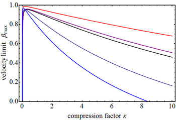
Figure 3 shows the maximum velocity  ${\rm \beta} _{{\rm max}}^{\rm e} (\varkappa _{\rm e} )$ from Eq. (12) exemplary for different materials. As one has an approximation of the compression while the acceleration, this map gives an overview over the maximum achievable velocity. For a better understanding, we will quantify this with a numerical example: Let us assume a laser with a pulse length of 65 fs, wavelength λ = 1 μm and an intensity of I 0 = 5 × 10²¹ W cm−2. The 25 nm-thick target consists of fully ionized titanium ions with Z = 22 and n i = 5.6 × 1028 m−3 and n e = 1.24 × 1030 m−3, n e ≈ 1100n c, respectively. Here, n c = ε0m eω2/e 2 is the critical electron density. If we postulate a compression of factor 2, this results in
 ${\rm \beta} _{{\rm max}}^{\rm e} \approx 0.75$ for the example above, which is in good agreement with simulation results. In the limit of high-compression (which can be expected), for example, ϰ e ≫ 1, Eq. (12) reduces to:
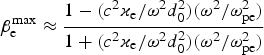 $${\rm \beta} _{\rm e}^{{\rm max}} \approx \displaystyle{{1 - (c^2 \varkappa _{\rm e} /{\rm \omega} ^2 d_0^2 )({\rm \omega} ^2 /{\rm \omega} _{{\rm pe}}^{\rm 2} )} \over {1 + (c^2 \varkappa_{\rm e} /{\rm \omega} ^2 d_0^2 )({\rm \omega} ^2 /{\rm \omega} _{{\rm pe}}^{\rm 2} )}}$$
If the laser propagation time decreases below the limit τEM ≤ 2τrelax/π, the maximum velocity drops below zero:  ${\rm \beta} _{{\rm max}}^{\rm e} \le 0$.
Shown is a map of  ${\rm \beta} _{{\rm max}}^{\rm e} $ [from Eq. (12)] as a function of the compression factor ϰ e for different materials: Hydrogen (black), carbon (purple), titanium (dark blue), gold 25 nm (red), and gold 10 nm (light blue).

One may understand this as follows: If we take the refractive index  $N^2 = 1 - {\rm \omega} _{{\rm pe}}^{\rm 2} /{\rm \omega} ^2 $, the velocity of light in the plasma is given by: c′ ≈ c/N. Under the condition ωpe ≫ ω, this reads: c′ ≈ cω/ωpe. Then τEM = 2d 0/c′ is the time, the laser pulse needs to propagate back and forth through the initial plasma. The above condition then states: If the penetration time τEM is of the order of the relaxation time of the electrons, Eq. (2) is violated and thus the quasi-static equilibrium can not establish. Descriptively this means, that if the penetration time of the laser pulse is much less than the relaxation time of the electron gas, the plasma is immediately transparent to the incident laser wave and the RPA mechanism will not start off. Therefore, one obtains from Eq. (2) a minimum target thickness required:
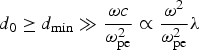 $$d_0 \ge d_{{\rm min}} \gg \displaystyle{{{\rm \omega} c} \over {{\rm \omega} _{{\rm pe}}^{\rm 2}}} \propto \displaystyle{{{\rm \omega} ^2} \over {{\rm \omega} _{{\rm pe}}^{\rm 2}}} {\rm \lambda}$$
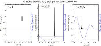
Note, the minimum target thickness depends on the target material and laser parameters (frequency and intensityFootnote 5). Figure 4 shows the plasma density distribution in the case, that the target got fully transparent while the acceleration process. From this we gain an important knowledge: The final kinetic energy of the plasma will not necessarily benefit from going to even higher laser intensities or thinner targets.
Spacial plasma distribution (full black line) for different times in the case, the target got fully transparent while the compression phase (left): After a phase of compression (middle), the incident laser wave (blue dashed line) penetrates the entire target and the plasma is rarefied (right). Note the axis scale! (From 1D PIC simulation, performed with VSim© Tech-X, 2015.)

5. MINIMIZATION OF THE ENERGY SPREAD
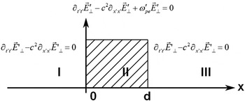
If one assumes the electron density to be initially a step function [see Eq. (10)], then it will remain such in an ideally co-moving system S′ for all timeFootnote 6. Therefore one has to treat the configuration shown in Figure 5: In the region of the electron density (II), the EM wave is described by Eq. (6), in the surrounding vacuum by the D'Alembert equation. Additional to that, it has to fulfill the continuity conditions:
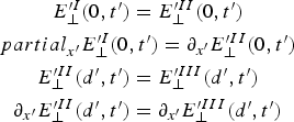 $$\displaylines{E_{\bot}^{\prime I} (0,t^{\prime}) = E_{\bot}^{\prime II} (0,t^{\prime}) \cr {partial} _{x^{\prime}} {E}_ \bot ^{\prime I} (0,t^{\prime}) = {\partial} _{x^{\prime}} E_ \bot ^{\prime II} (0,t^{\prime}) \cr E_ \bot ^{\prime II} (d{^\prime},t{^\prime}) = E_ \bot ^{\prime III} (d{^\prime},t{^\prime}) \cr {\partial} _{x^{\prime}} E_ \bot ^{\prime II} (d{^\prime},t{^\prime}) = {\partial} _{x^{\prime}} E_ \bot ^{\prime III} (d{^\prime},t{^\prime})}$$
To solve this problem, we make a Fourier transformation (Strauss, Reference Strauss1995) of the electrical field components and give the solution in the frequency domain. We introduce the wave numbers in the three regions as:  $k^{\prime}_{\rm I} (\Omega ^{\prime}) = \Omega ^{\prime}/c$,
 $k_{{\rm II}}^{^{\prime}2} (\Omega^{\prime})$
 $ = 1/c^2(\Omega ^{2^{\prime}} - {\rm \omega} _{{\rm pe}}^{{\rm 2^{\prime}}} ),$ and
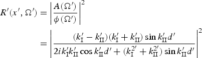
 $k^{\prime}_{{\rm III}} (\Omega^{\prime}) = \Omega ^{\prime}/c$. ϕ(Ω′) is the Fourier transformed of the incident laser wave and A(Ω′) is the amplitude of the reflected wave. We note that, since the EM signal propagates with c, the time between the three regions is shiftedFootnote 7. If we refer to the Fourier transformed of the electrical field, we will denote it with Fk(x′, Ω′), with k = I, II, III for the respective region. Solving the problem shown in Figure 5 for the reflection index R′(Ω′) = |A(Ω′)/ϕ(Ω′)| 2 givesFootnote 8:
 $$\eqalign{R^{\prime}(x^{\prime},\Omega^{\prime}) = & \left\vert {\displaystyle{{A(\Omega ^{\prime})} \over {{\rm \phi} (\Omega ^{\prime})}}} \right\vert^2 \cr = & \left\vert {\displaystyle{{(k^{\prime}_{\rm I} - k^{\prime}_{{\rm II}} )(k^{\prime}_{\rm I} + k^{\prime}_{{\rm II}} )\sin k^{\prime}_{{\rm II}} d^{\prime}} \over {2ik^{\prime}_{\rm I} k^{\prime}_{{\rm II}} \cos k^{\prime}_{{\rm II}} d^{\prime} + (k_{\rm I}^{2^{\prime}} + k_{{\rm II}}^{2^{\prime}} )\sin k^{\prime}_{{\rm II}} d^{\prime}}}} \right\vert^2}$$
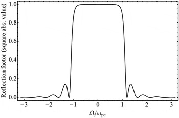
Figure 6 shows the reflection index as a function of the frequency R′(Ω′) = |A(Ω′)/ϕ(Ω′)| 2. In the range  $\left\vert {\Omega ^{\prime}} \right\vert \lt {\rm \omega} _{{\rm pe}}^{\rm ^{\prime}} $ it is nearly constant, R ≈ 1, but for
 $\left\vert {\Omega ^{\prime}} \right\vert \gt {\rm \omega} _{\rm pe}^{\prime} $ it decreases rapidly and behaves like a nonlinear Fabri–Peròt–Etalon. Moreover, the reflective index depends on the thickness of the plasma slab, R = R(d). Thus, if the thickness tends to zero, d→0, the reflective index will shrink to zero, too. This also validates the predictions of the first section.
Configuration of the model: The incident laser wave propagates from the left to the right through the vacuum region I. Region II is the plasma slab, which can be described by Eq. (6). After the penetration of the plasma, the EM wave enters vacuum again (region III)

Reflection index R = |A/φ| 2 as a function of Ω/ωpe for d = 5δ [from Eq. (16)].

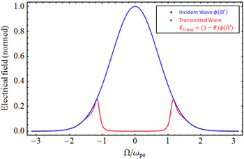
Since  $E_\bot^{\rm \prime II} = (1 - R){\rm \phi} (\Omega ^{\prime})$, the high-frequency parts of the incident laser pulse are transmitted through the plasma. This is qualitatively shown in Figure 7 for the case of a Gaussian-sine laser amplitude. From Eq. (4) follows:
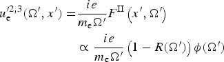 $$\eqalign{u_{\rm e}^{\prime 2,3} (\Omega ^{\prime},x^{\prime}) = & \displaystyle{{ie} \over {m_{\rm e} \Omega ^{\prime}}}F^{{\rm II}} \left( {x^{\prime },\Omega^{\prime }} \right) \cr & \propto \displaystyle{{ie} \over {m_{\rm e} \Omega ^{\prime}}}\left( {1 - R(\Omega ^{\prime})} \right){\rm \phi} (\Omega ^{\prime})}$$
Equation (17) together with the transmission coefficient T = 1–R can be understood as follows: For each frequency Ω′ of the incident laser pulse which is transmitted through the plasma slab, there exists a particular azimuthal velocity  $u_{\rm e}^{^{\prime}2,3} (\Omega ^{\prime})$. But since the longitudinal velocity depends on the product
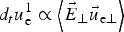 $d_t u_{\rm e}^{\rm 1} \propto \left\langle {\vec E_ \bot \vec u_{{\rm e} \bot}} \right\rangle $, for different transmitted frequencies there will be different longitudinal velocities. This effect leads to the velocity spread in the RPA mechanism. To minimize the velocity spread it is therefore necessary to minimize the amount of transmitted laser energy. One can achieve this goal by choosing an incident laser signal, which should be in the range −ωpe < Ω′ < ωpe, since in this range R ≈ 1 and the entire wave is reflected (compare with Fig. 6). Signals which have |Ω′| > |ω pe| will cause higher velocity spread.
Incident wave amplitude φ(Ω′) (blue line) and transmitted wave amplitude  $E_ \bot ^{\prime II} = (1 - R){\rm \phi} (\Omega ^{\prime})$ (full red line) as functions of Ω/ωpe. The high-frequency parts of the wave are entirely transmitted since R vanishes for those frequencies.

From the properties of the Fourier transformation it is known, that a signal short in time domain leads to a broad signal in frequency domain and a signal only, slowly varying in time leads to a narrow frequency band. For the optimization of the RPA process this means: If one lets the energy density
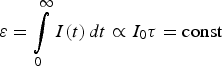 $${\rm \varepsilon} = \int\limits_0^\infty {I(t)\,dt \propto I_0 {\rm \tau} = {\rm const}}$$
of the entire laser pulse constant, but changes the intensity and pulse length such that I 0τ = const, then the signal with the longer pulse length will result in a smaller velocity spread. Precisely speaking this means: A longer laser pulse with a lower intensity results in a more narrow energy distribution than a shorter one with a higher intensity, while the mean kinetic energy  $\bar E_{{\rm kin}} $ of the plasma will remain nearly the same in both cases.
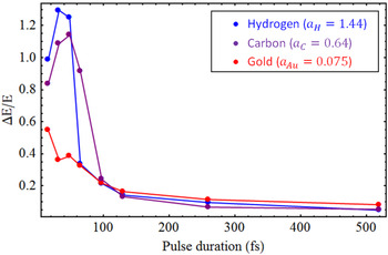
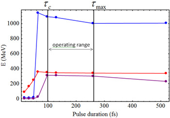
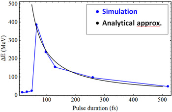
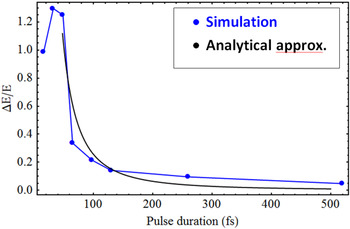
To validate these predictions, 1D PIC simulations are performed for different parameters. This also gives the opportunity to quantify the optimization. We chose three different materials for the targets: Gold (density ρAu = 19320 kg m−3) with a charge of Z = +15, fully ionized carbon (density ρC = 2260 kg m−3) and fully ionized hydrogen with a density of ρH = 1000 kg m−3. All targets have an initial thickness of d 0 = 25 nmFootnote 9. The laser pulse length is chosen in the range τ = 16−260 fs, the corresponding intensity I 0 = 1.25 × 10²¹−2 × 10²² W cm−2. Thereby the leading acceleration parameter a 0 = I 0τ/(ρd 0c 2) remains constant. This leads to the following acceleration parameters: a 0Au = 0.075, a 0C = 0.64, and a 0H = 1.44. Figure 8 shows the energy spread ΔE relative to the mean energy  $\bar E$ as a function of the pulse length. As predicted by theory [Eqs. (6) and (16)], the velocity spread decreases with increasing pulse length (for more details, see Appendix). The achieved mean kinetic energy of the plasma is shown in Figure 9: For a wide range of pulse length, the mean kinetic energy is nearly equal. Therefore the optimum working point for the RPA is at the right-hand side of the energy plateau, where the mean kinetic energy has a maximum, but the energy spread has a minimum (Figs. 8 and 9). One can obtain even more information from Figures 8 and 9: Below a certain threshold pulse length, τL < τc (see Fig. 9, τc ≈ 50−60 fs), the mean kinetic energy
 $\bar E$ decreases rapidly. In that case, τL ≅ 60 fs, the condition from Eq. (1) is violated and the RPA will not start at all. From the purple curve in Figure 9 one adopts, that the RPA will also break down in the case of too low laser intensities, even for long pulse lengths, since the mean kinetic energy decreases again from a certain point on.
Shown is the ratio of the energy spread and the mean kinetic energy  $\Delta E_{{\rm kin}} /\bar E_{{\rm kin}} $. As predicted by the theory [Eqs. (16) and (17)], it decreases rapidly with increasing laser pulse length. For the materials: Carbon (blue), gold (red), and hydrogen (purple). (From 1D PIC simulation, performed with VSim© Tech-X, 2015.)

Mean kinetic energy  $\bar E_{{\rm kin}} $ as a function of the laser pulse length. Below a threshold pulse length τc ≈ 50–60 fs,
 $\bar E_{{\rm kin}} $ decreases rapidly. For the materials: Carbon (blue), gold (red), and hydrogen (purple). As can be seen from the purple curve, above a certain pulse length of the mean kinetic energy decreases again, since the intensity gets too low to start a radiation pressure acceleration. This gives rise to the presumption, that there has to be an upper limitation. (From 1D PIC simulation, performed with VSim© Tech-X, 2015.)

6. CONCLUSIONS AND OUTLOOK
A relativistic two fluid model was derived for the coupling of the laser wave with a plasma slab. From this model two important principles have been obtained: A termination criterion for the acceleration process was worked out, stating that the plasma beam will not necessarily benefit from going to even higher laser intensities or thinner targets. Within this criterion, the maximum achievable kinetic energy of the plasma could be estimated. It was shown that for even higher laser intensities the RPA mechanism collapses. Furthermore, a formula for the minimum target thickness in terms of the target material and laser parameters (frequency and intensity) was calculated. In the second stage, the reflection index of the plasma was derived in the frequency domain. From that, we gain an important perception for the optimization of the RPA: Longer laser pulses with lower intensities cause smaller energy spread than short pulses of high-intensity. The analytical predictions have been validated by 1D PIC simulations. From these results, the optimum working point for the RPA was estimated. The operating range for the RPA is limited to a certain pulse length τL∈(τc, τmax) and a minimum intensity. For shorter pulse lengths τL < τc ≈ 60 fs, the RPA mechanism does not start off. The resulting energy spread could be assessed by an analytical scaling law that depends on the laser pulse length and intensity. All the results were generated for the case of a circular polarized laser. The radiation pressure acceleration also works for a linear polarized laser, but this will cause more electron heating. Thus the expected energy spectra will be more broadened. In Kim et al. (Reference Kim, Pae, Kim, Kim, Lee, Choi, Singhal, Sung, Lee, Lee, Nickles and Nam2014), experimental results for the RPA of ultra thin polymer targets were performed. The experimentally achieved results are in good agreement with the theoretical predictions and thus validate the model presented in this work. Especially the scaling laws observed in the experiment agree with those from the relativistic two fluid model. As a next step, a perturbation theory in the moving frame S′ will reveal more information about the two limits of the RPA. Additional to that, two-dimensional PIC simulations will be carried out to analyze the effect of higher dimensions. It can be predicted, that the curved laser profile will result in an outflow of mass from the plasma center toward the outer plasma wings. This outflow causes a rarefaction of the plasma center, which will in some cases result in a hole boring.
ACKNOWLEDGEMENTS
We thank Professor Dr. Wolfgang Ellermeier for his advisory help and for critical reading of this paper. The work was supported by HIC for FAIR and HGS HIRe.
APPENDIX
Statement: Consider a system moving with v(x, t) and a system moving with v = const. The deviations of both systems with respect to Lorentz transformation is of higher order and negligible.
Proof: For a system moving with v = const the Lorentz transformation satifies the metric:
 $$ds^2 = {\rm \eta} _{{\rm \alpha} {\rm \beta}} dx^{\rm \alpha} dx^{\rm \beta} = c^2 dt^2 - dx^2 = c^2 dt^{{\prime}2} - dx^{{\prime}2}$$
For simplicity we will only treat a 1D system, but this derivation can be generalized to three dimensions. In a system moving with v = v(x, t) (e.g., an accelerated system), the Lorentz-transformation does not remain linear. Instead, the differentials read:
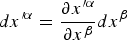 $$dx^{\prime {\rm \alpha}} = \displaystyle{{\partial x^{\prime{\rm \alpha}}} \over {\partial x^{\rm \beta}}} dx^{\rm \beta} $$
Thus, the metrical tensor itself depends on the variables xα. Furthermore it holds:
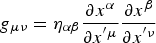 $$g_{{\rm \mu} {\rm \nu}} = {\rm \eta} _{{\rm \alpha} {\rm \beta}} \displaystyle{{\partial x^{\rm \alpha}} \over {\partial x^{^{\prime}{\rm \mu}}}} \displaystyle{{\partial x^{\rm \beta}} \over {\partial x^{^{\prime}{\rm \nu}}}}$$
and
 $$ds^2 = g_{{\rm \mu} {\rm \nu}} dx^{\prime {\rm \mu}} dx^{\prime {\rm \nu}}$$
Let us now explicitly derive the metric in one spacial dimension. The coordinates in the laboratory frame are given as:
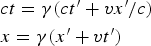 $$\eqalign{& ct = {\rm \gamma} (ct^{\prime} + vx^{\prime}/c) \cr & x = {\rm \gamma} (x^{\prime} + vt^{\prime})} $$
And let v = v(x′, t′) depend on the space-time variables. Then the entries of the metrical tensor are given by the partial derivatives of the coordinates, thus they read:
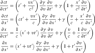 $$\eqalign{\displaystyle{\partial ct \over \partial ct^{\prime}} & = \left(t^{\prime} + \displaystyle{vx^{\prime} \over c^2} \right) \displaystyle{\partial {\rm \gamma} \over \partial v} \displaystyle{\partial v \over \partial t^{\prime}} + {\rm \gamma} \left(1 + \displaystyle{x^{\prime} \over c^2} \displaystyle{\partial v \over \partial t^{\prime}} \right) \cr \displaystyle{\partial ct \over \partial x^{\prime}} & = \left(ct^{\prime} + \displaystyle{vx^{\prime} \over c} \right) \displaystyle{\partial {\rm \gamma} \over \partial v} \displaystyle{\partial v \over \partial x^{\prime}} + {\rm \gamma} \left(\displaystyle{v \over c} + \displaystyle{x^{\prime} \over c} \displaystyle{\partial v \over \partial x^{\prime}} \right) \cr \displaystyle{\partial x \over \partial ct^{\prime}} &= \displaystyle{1 \over c}\left(x^{\prime} + vt^{\prime} \right)\displaystyle{\partial {\rm \gamma} \over \partial v} \displaystyle{\partial v \over \partial t^{\prime}} + {\rm \gamma} \left(\displaystyle{v \over c} + \displaystyle{1 \over c}\displaystyle{\partial v \over \partial t^{\prime}} t^{\prime} \right) \cr \displaystyle{\partial x \over \partial x^{\prime}} &= \left(x^{\prime} + vt^{\prime} \right) \displaystyle{\partial {\rm \gamma} \over \partial v} \displaystyle{\partial v \over \partial x^{\prime}} + {\rm \gamma} \left(1 + t^{\prime}\displaystyle{\partial v \over \partial x^{\prime}} \right)}$$
Let τ′∝1/ω be the long time scale of the laser pulse and t′∝1/ωpe be the time scale of the fast electron oscillations. Since τ′ ≫ t′ we may write t′ = ετ′, with a small number ε ≪ 1. Let us now split the velocity into two parts: v = β0c + εc. The barycentrically velocity v 0 = β0(τ′)c varies on the laser time scale and describes the movement of the plasma center. The second term ε(x′, t′)c varies on the short time scale of the plasma oscillations and describes the drifts. For the RPA we can assume, that ε ≪ β0 and therefore  ${\rm \gamma} \approx {\rm \gamma} _0 + {\rm \varepsilon} {\rm \gamma} _0^3 {\rm \beta} _0 $. Moreover, we know that the barycentric velocity does not change much on the time scale of plasma oscillations, meaning that
 $$\displaystyle{{\partial v} \over {\partial t^{\prime}}} \approx \varepsilon $$
holds. The RPA runs on the length scale of the laser wavelength λ. The velocity spread on the other hand is based on the scale of the penetration-depth δ ≈ c/ωpe ≪ λ. Therefore x′∝ελ is justified on the short time scale. Under compliance of the chain rule and the assumptions made, the derivatives re-write to:
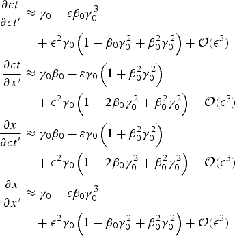 $$\eqalign{\displaystyle {\partial ct \over \partial ct^{\prime}} & \approx {\rm \gamma} _0 + {\rm \varepsilon} {\rm \beta} _0 {\rm \gamma} _0^3 \cr & \quad + {\rm \epsilon} ^2 {\rm \gamma} _0 \left( {1 + {\rm \beta} _0 {\rm \gamma} _0^2 + {\rm \beta} _0^2 {\rm \gamma} _0^2} \right) + {\rm \cal O}({\rm \epsilon} ^3 ) \cr \displaystyle{\partial ct \over \partial x^{\prime}} &\approx {\rm \gamma} _0 {\rm \beta} _0 + {\rm \varepsilon} {\rm \gamma} _0 \left( {1 + {\rm \beta} _0^2 {\rm \gamma} _0^2} \right) \cr & \quad + {\rm \epsilon} ^2 {\rm \gamma} _0 \left( {1 + 2{\rm \beta} _0 {\rm \gamma} _0^2 + {\rm \beta} _0^2 {\rm \gamma} _0^2} \right) + {\rm \cal O}({\rm \epsilon} ^3 ) \cr \displaystyle {\partial x \over \partial ct^{\prime}} &\approx {\rm \gamma} _0 {\rm \beta} _0 + {\rm \varepsilon} {\rm \gamma} _0 \left( {1 + {\rm \beta} _0^2 {\rm \gamma} _0^2} \right) \cr & \quad + {\rm \epsilon} ^2 {\rm \gamma} _0 \left( {1 + 2{\rm \beta} _0 {\rm \gamma} _0^2 + {\rm \beta} _0^2 {\rm \gamma} _0^2} \right) + {\rm \cal O} ({\rm \epsilon} ^3 ) \cr \displaystyle{\partial x \over \partial x^{\prime}} &\approx {\rm \gamma} _0 + {\rm \varepsilon} {\rm \beta} _0 {\rm \gamma} _0^3 \cr & \quad + {\rm \epsilon} ^2 {\rm \gamma} _0 \left( {1 + {\rm \beta} _0 {\rm \gamma} _0^2 + {\rm \beta} _0^2 {\rm \gamma} _0^2} \right) + {\rm \cal O}({\rm \epsilon} ^3 )}$$
The transformation matrix can be expanded to:
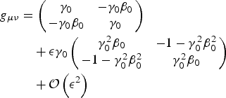 $$\eqalign{g_{{\rm \mu} {\rm \nu}} &= \left(\matrix{{\rm \gamma} _0 & - {\rm \gamma} _0 {\rm \beta} _0 \cr - {\rm \gamma} _0 {\rm \beta} _0 & {\rm \gamma} _0} \right) \cr & \quad+ {\rm \epsilon} {\rm \gamma} _0 \left(\matrix{{\rm \gamma} _0^2 {\rm \beta} _0 & - 1 - {\rm \gamma} _0^2 {\rm \beta} _0^2 \cr - 1 - {\rm \gamma} _0^2 {\rm \beta} _0^2 & {\rm \gamma} _0^2 {\rm \beta} _0} \right) \cr &\quad + {\cal O} \left({\rm \epsilon} ^2 \right)}$$
It follows that the deviations from the linear Lorentz transformation are of the order of  ${\rm \cal O}({\rm \epsilon} )$ and higher and thus negligible small. ■
Full solution of Section 2: A Fourier transformation of the electrical field components can be given as:
 $$F^k \left( {x^{\prime},\Omega^{\prime}} \right) = \displaystyle{1 \over {\sqrt {2{\rm \pi}}}} \int\limits_{ - \infty} ^\infty {E^k (x^{\prime},t^{\prime})e^{ - it^{\prime} \Omega ^{\prime}} dt^{\prime}}$$
With the typical exponential Ansatz we then get:
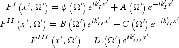 $$\displaylines{F^I \left( {x^{\prime},\Omega^{\prime}} \right) = {\rm \phi} \left( {\Omega ^{\prime}} \right)e^{ik^{\prime}_I x^{\prime}} + A\left( {\Omega ^{\prime}} \right)e^{ - ik^{\prime}_I x^{\prime}} \cr F^{II} \left( {x^{\prime},\Omega^{\prime}} \right) = B\left( {\Omega ^{\prime}} \right)e^{ik^{\prime}_{II} x^{\prime}} + C\left( {\Omega ^{\prime}} \right)e^{ - ik^{\prime}_{II} x^{\prime}} \cr F^{III} \left( {x^{\prime},\Omega^{\prime}} \right) = D\left( {\Omega ^{\prime}} \right)e^{ik^{\prime}_{III} x^{\prime}}} $$
The full solution of the problem is shown in Figure 5 and Eqs. (15) and (A11) in the frequency domain gives:
 $$\eqalign{F^I \left( {x^{\prime},\Omega^{\prime}} \right) = & {\rm \phi} \left( {\Omega ^{\prime}} \right)e^{ik^{\prime}_I x^{\prime}} \cr & + \displaystyle{{{\rm \phi} \left( {\Omega ^{\prime}} \right)\left( {k^{\prime}_I - k^{\prime}_{II}} \right)\left( {k^{\prime}_I + k^{\prime}_{II}} \right)\sin k^{\prime}_{II} d^{\prime}} \over {2ik^{\prime}_I k^{\prime}_{II} \cos k^{\prime}_{II} d^{\prime} + \left( {k_I^{2^{\prime}} + k_{II}^{2^{\prime}}} \right)\sin k^{\prime}_{II} d^{\prime}}}e^{ - ik^{\prime}_I x^{\prime}}}$$
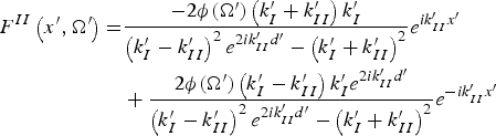 $$\eqalign{F^{II} \left( {x^{\prime},\Omega^{\prime}} \right) = & \displaystyle{{ - 2{\rm \phi} (\Omega ^{\prime})\left( {k^{\prime}_I + k^{\prime}_{II}} \right)k^{\prime}_I} \over {\left( {k^{\prime}_I - k^{\prime}_{II}} \right)^2 e^{2ik^{\prime}_{II} d^{\prime}} - \left( {k^{\prime}_I + k^{\prime}_{II}} \right)^2}} e^{ik^{\prime}_{II} x^{\prime}} \cr & + \displaystyle{{2{\rm \phi} (\Omega ^{\prime})\left( {k^{\prime}_I - k^{\prime}_{II}} \right)k^{\prime}_I e^{2ik^{\prime}_{II} d^{\prime}}} \over {\left( {k^{\prime}_I - k^{\prime}_{II}} \right)^2 e^{2ik^{\prime}_{II} d^{\prime}} - \left( {k^{\prime}_I + k^{\prime}_{II}} \right)^2}} e^{ - ik^{\prime}_{II} x^{\prime}}} $$
 $$F^{III} \left( {x^{\prime},\Omega^{\prime}} \right) = \displaystyle{{2i{\rm \phi} (\Omega ^{\prime})e^{ - ik^{\prime}_I d^{\prime}} k^{\prime}_I k^{\prime}_{II}} \over {2ik^{\prime}_I k^{\prime}_{II} \cos k^{\prime}_{II} d^{\prime} + \left( {k_I^{2^{\prime}} + k_{II}^{2^{\prime}}} \right)\sin k^{\prime}_{II} d^{\prime}}}e^{ik^{\prime}_I x^{\prime}} $$
Analytical scaling law for the plasma energy spread: For simplicity, let us assume a plasma half-space, that is: d→∞. Then, τEM→∞ holds and thus, the conditions 1 and 2 are satisfied. Furthermore we introduce a simple laser model:
 $$E_{\rm L} (t) = A_0 \displaystyle{{4t^2} \over {{\rm \tau} _{\rm L}^2}} \exp ( - 4t^2 /{\rm \tau} _{\rm L}^2 + 1)$$
Acoording to the Plancherel formula it holds:
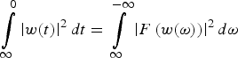 $$\int\limits_\infty ^0 {\left\vert {w(t)} \right\vert^2 dt} = \int\limits_\infty ^{ - \infty} {\left\vert {F\left( {w({\rm \omega} )} \right)} \right\vert^2 d{\rm \omega}}$$
where w(ω) = ε0T(ω)E 2(ω) is the transmitted energy density of the laser wave and T(ω) = 1−R(ω) is the frequency-depended transmission coefficient. From this we gain two interesting scaling laws for the plasma energy spread:
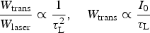 $$\displaystyle{{W_{{\rm trans}}} \over {W_{{\rm laser}}}} \propto \displaystyle{1 \over {{\rm \tau} _{\rm L}^2}}, \quad W_{{\rm trans}} \propto \displaystyle{{I_0} \over {{\rm \tau} _{\rm L}}}$$
Figures 10 and 11 show a comparison of this scaling laws with simulation results. In the range, where the assumptions hold, they are in well agreement.
(Colour online) Energy spread of the RPA plasma as a function of the laser pulse length.(From 1D PIC simulation, performed with VSim© Tech-X, 2015.)

(Colour online) Energy spread relative to the mean kinetic energy of an RPA plasma.(From 1D PIC simulation, performed with VSim© Tech-X, 2015.)