1. Introduction
In the last three decades, significant attention has been devoted to improving knowledge of the hydrodynamic processes that occur in the surf zone, and in particular the breaking of waves. It is generally accepted that breaker types can be classified as a continuous spectrum from spilling to surging, depending on the initial wave steepness and the bed slope. The general processes involved in wave steepening and subsequent breaking are now well known and have been fully described by numerous authors (Peregrine Reference Peregrine1983; Kiger & Duncan Reference Kiger and Duncan2012). Nevertheless, the wave breaking phenomenon remains a very challenging fluid mechanics problem, with turbulence and aeration interactions making it more difficult to investigate in detail.
Depending on the type of breaker, three types of large-scale coherent vortices can be found in breaking waves (Zhang & Sunamura Reference Zhang, Sunamura and Edge1994). The jet-splash cycles, occurring several times in a single plunging breaker, are responsible for the generation of a sequence of large-scale vortices with a horizontal axis of rotation (Bonmarin Reference Bonmarin1989; Kimmoun & Branger Reference Kimmoun and Branger2007). Some of these eddies have been shown to be co-rotating vortices and some counter-rotating vortices. In the case of spilling breakers, Nadaoka, Hino & Koyano (Reference Nadaoka, Hino and Koyano1989) detailed the flow field under a turbulent bore propagating towards the shoreline. Large dominant horizontal eddies are present in the bore front, while behind the wave crest the flow structure changes rapidly into obliquely downward stretched three-dimensional (3D) eddies, so-called ‘obliquely descending eddies’. More recently, Kubo & Sunamura (Reference Kubo and Sunamura2001) revealed that a new type of large-scale turbulence, named the ‘downburst’, is present in the breaker zone along with the previously observed oblique vortex. It is characterised by a descending water mass without marked rotational features, diverging at the bed and agitating sediment particles more vigorously than the oblique vortices. Ting (Reference Ting2006) also identified these downbursts of turbulence descending from the free surface. Very few numerical works have been dedicated to reproducing these 3D large features, which occur when waves break (Watanabe & Saeki Reference Watanabe and Saeki1999; Christensen & Deigaard Reference Christensen and Deigaard2001; Watanabe, Saeki & Hosking Reference Watanabe, Saeki and Hosking2005; Christensen Reference Christensen2006; Lubin et al. Reference Lubin, Vincent, Abadie and Caltagirone2006; Lakehal & Liovic Reference Lakehal and Liovic2011). Watanabe & Saeki (Reference Watanabe and Saeki1999) investigated the 3D distribution and time variation of rotating components of velocity induced by wave breaking. They showed that two-dimensional (2D) large eddy motions generated by wave breaking rapidly broke down to fully 3D flow structures during splash-up cycle as waves propagate on the sloping beach. Christensen & Deigaard (Reference Christensen and Deigaard2001) found similar results, showing that 3D flow structures spontaneously developed at the breaking point, and identified the formation of obliquely descending eddies. Nevertheless, these obliquely descending eddies were not always found to occur, longitudinal eddies with horizontal axes being observed instead.
Major discussion about the generation of turbulent structures and their interactions was continued by Watanabe et al. (Reference Watanabe, Saeki and Hosking2005). Spilling, plunging, strongly plunging and spilling/plunging breakers were simulated. The 2D structure of the flow was found to evolve in streamwise 3D vortices, owing to a local shear instability analogous to Kelvin–Helmholtz (KH) instability. Vorticity was shown to be unstable in a saddle region localised between the rebounding plunging jet and the primary spanwise vortex formed by the initial free-falling tongue of water ejected from the crest of the breaking wave. The first splash-up rebounded and induced another main spanwise vortex. Between the first primary spanwise vortex and this latest one, a vortex loop took place, undulated and wrapped the adjacent primary vortices to form a rib structure. Watanabe et al. (Reference Watanabe, Saeki and Hosking2005) speculated that this structure could be the obliquely descending eddies observed by Christensen & Deigaard (Reference Christensen and Deigaard2001). The impact of these various structures on the free-surface aspect was also illustrated. Finally, the formation of obliquely descending eddies and the subsequent air entrainment was investigated. Lakehal & Liovic (Reference Lakehal and Liovic2011) presented pictures showing surface deformations similar to those identified by Watanabe et al. (Reference Watanabe, Saeki and Hosking2005) for plunging breakers.
A limited number of researchers have also focused attention on smaller-scale processes, such as the degeneration of gravity-dominated jets (e.g. pre-impact plunging jets) to scars, droplets and spray (Longuet-Higgins Reference Longuet-Higgins1995; Watanabe et al. Reference Watanabe, Saeki and Hosking2005; Lakehal & Liovic Reference Lakehal and Liovic2011). Narayanaswamy & Dalrymple (Reference Narayanaswamy, Dalrymple and Smith2002) experimentally presented evidence of ‘fingers’ appearing at the tip of the plunging jet, prior to impact. More recently, Saruwatari, Watanabe & Ingram (Reference Saruwatari, Watanabe and Ingram2009) numerically studied the formation of fingers and scars on the surface of secondary planar jets and suggested that, as the influence of surface tension increases, the jet surface is prevented from being scarified and fingered. Handler, Savelyev & Lindsey (Reference Handler, Savelyev and Lindsey2012) experimentally investigated the generation of coherent elongated structures behind breaking waves. These streaks were shown to appear when the crest of a strong breaker interacts with pre-existing turbulence induced by weaker pre-breakers, suggesting that a wave–turbulence interaction process could be responsible for streak generation.
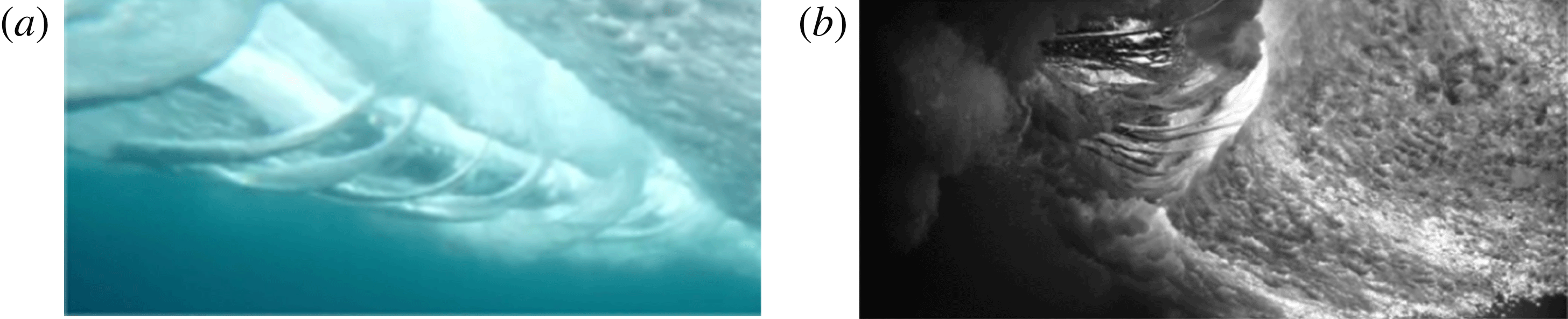
On 6 May 2009, BBC Worldwide released a short clip of a large breaking wave filmed in slow motion (BBC 2009). The high-definition film caught the attention and curiosity of the scientific community. The video has attracted extremely positive reactions on the video-sharing website YouTube (more than 4.8 million views at the time of writing). The beautiful breaking wave, filmed from underwater, revealed for the first time 3D coherent structures: some beautiful large aerated vortex filaments, bathtub-like or tornado-like vortices, elongated in the main flow direction, connecting the splash-up and the main tube of air (figure 1).
Plunging breaking waves filmed from underwater. As the waves break and move forwards, air is entrained and carried along, causing unusual underwater tornado-like vortical tubes wrapping around the tube. What you see in both pictures is the tube rolling towards the shoreline from left to right. On the far right is the white water caused by the impact of the lip. Pictures used with kind permission of underwater cinematographers (a) Chris Bryan and (b) Mark Tipple (http://www.theunderwaterproject.com).

Performing numerical simulations of 3D breaking waves requires a large number of mesh grid nodes, robust and accurate numerical methods, and long CPU time calculations in order to compute the hydrodynamics from the largest to the smallest length and time scales (Lubin et al. Reference Lubin, Glockner, Kimmoun and Branger2011). Recent progress in computational power has allowed us to run fine 3D simulations, which gave us the opportunity to study, for the first time, the fine vortex filaments generated during the early stage of the plunging wave breaking process, and the subsequent air entrainment. The aim of this paper is to present the first study of these coherent eddy structures. The numerical results will be detailed to educe and explain the formation and evolutionary dynamics of the vortex filaments, and to explore the role of eddies in the air entrainment process.
2. Numerical model
2.1. Governing equations and numerical methods
An incompressible multiphase flow between non-miscible fluids can be described by the Navier–Stokes equations in the single-fluid formulation (Kataoka Reference Kataoka1986). The governing equations for the large-eddy simulation (LES) are classically derived by applying a convolution filter to the unsteady Navier–Stokes equations. The resulting set of equations describes the entire hydrodynamic and geometrical processes involved in the motion of multiphase media (2.1)–(2.3):
 $$\begin{eqnarray}\displaystyle & \boldsymbol{{\rm\nabla}}\boldsymbol{\cdot }\boldsymbol{u}=0, & \displaystyle\end{eqnarray}$$
 $$\begin{eqnarray}\displaystyle & \displaystyle {\it\rho}\left(\frac{\partial \boldsymbol{u}}{\partial t}+\boldsymbol{u}\boldsymbol{\cdot }\boldsymbol{{\rm\nabla}}\boldsymbol{u}\right)=-\boldsymbol{{\rm\nabla}}p+{\it\rho}\boldsymbol{g}+\boldsymbol{{\rm\nabla}}\boldsymbol{\cdot }(({\it\mu}+{\it\mu}_{t})[\boldsymbol{{\rm\nabla}}\boldsymbol{u}+\boldsymbol{{\rm\nabla}}^{t}\boldsymbol{u}]) & \displaystyle\end{eqnarray}$$
 $$\begin{eqnarray}\frac{\partial C}{\partial t}+\boldsymbol{u}\boldsymbol{\cdot }\boldsymbol{{\rm\nabla}}C=0,\end{eqnarray}$$
where
 $\boldsymbol{u}$
is the velocity,
 $C$
the phase function,
 $t$
the time,
 $p$
the pressure,
 $\boldsymbol{g}$
the gravity vector,
 ${\it\rho}$
the density and
 ${\it\mu}$
the dynamic viscosity. The turbulent viscosity
 ${\it\mu}_{t}$
is calculated with the mixed scale model (Sagaut Reference Sagaut1998). Here
 $x$
,
 $z$
and
 $y$
are respectively the horizontal, vertical and transverse coordinates; and
 $u_{x}$
,
 $u_{z}$
and
 $u_{y}$
are the corresponding velocity components of the velocity vector
 $\boldsymbol{u}$
. Surface tension is not considered in this study, as discussed in § 3.5. The magnitude of the physical characteristics of the fluids depends on the local phase. They are defined according to
 $C$
in a continuous manner as
 $$\begin{eqnarray}\displaystyle \left.\begin{array}{@{}c@{}}{\it\rho}=C{\it\rho}_{w}+(1-C){\it\rho}_{a},\\ {\it\mu}=C{\it\mu}_{w}+(1-C){\it\mu}_{a},\end{array}\right\} & & \displaystyle\end{eqnarray}$$
where
 ${\it\rho}_{a}$
,
 ${\it\rho}_{w}$
,
 ${\it\mu}_{a}$
and
 ${\it\mu}_{w}$
are the densities and viscosities of air and water, respectively.
Time discretisation of the momentum equation is implicit and an Euler scheme is used. The velocity–pressure coupling under the incompressible flow constraint is solved with the time splitting pressure correction method (Goda Reference Goda1979). The equations are discretised on a staggered grid by means of the finite volume method. The space derivatives of the inertial term are discretised by a hybrid upwind-centred scheme, whereas the viscous term is approximated by a second order centred scheme.
The interface tracking is achieved by a volume-of-fluid (VOF) method and a piecewise linear interface calculation (PLIC) (Youngs Reference Youngs, Morton and Baines1982; Scardovelli & Zaleski Reference Scardovelli and Zaleski1999). This method has the advantage of building a sharp interface between air and water. A phase function
 $C$
is used to locate the different fluids. It is classically smoothed into
 $\widetilde{C}$
before the calculation of the physical properties (density and viscosity) is made, using an inverse distance weighting average. The variation of the fluid properties are then diffused over 2–6 cells, depending of the breaking wave type and meshes. Finally, since the phase function is not defined at each point where viscosities and densities are needed for the Navier–Stokes discretisation, the physical characteristics are interpolated on the staggered grid. We use a linear interpolation to calculate the density on the velocity nodes, whereas a harmonic interpolation is used for the viscosity.
The MPI library is used to parallelise the code. The mesh is partitioned into equal size subdomains to ensure load balancing. Communications between processors are also minimised (Ahusborde & Glockner Reference Ahusborde and Glockner2011). The HYPRE parallel solver and preconditioner library is used to solve the linear systems (Falgout, Jones & Yang Reference Falgout, Jones, Yang, Bruaset and Tveito2006). The numerical code has already been extensively verified and validated through numerous test cases, including mesh refinement analysis (Lubin et al. Reference Lubin, Vincent, Abadie and Caltagirone2006; Lubin, Chanson & Glockner Reference Lubin, Chanson and Glockner2010; Lubin et al. Reference Lubin, Glockner, Kimmoun and Branger2011; Poux, Glockner & Azaiez Reference Poux, Glockner and Azaiez2011; Brouilliot & Lubin Reference Brouilliot and Lubin2013). The accuracy of the numerical schemes and the conservation laws of mass and energy in the computational domain have been accurately verified.
2.2. Definition of the initial conditions and parameters
We use initial conditions corresponding to a single unstable periodic sinusoidal wave of large amplitude. This somewhat artificial wave breaking configuration has already been documented in several previous studies and proved to be effective at simulating all types of breaking waves (Abadie, Caltagirone & Watremez Reference Abadie, Caltagirone and Watremez1998; Chen et al. Reference Chen, Kharif, Zaleski and Li1999; Lubin et al. Reference Lubin, Vincent, Abadie and Caltagirone2006; Iafrati Reference Iafrati2009).
The rectangular calculation domain is periodic in the wave propagation direction and one wavelength long. A free-slip boundary condition is imposed at the lower limit, and an absorption boundary condition at the upper limit. The reference variables of the initial incident wave are the celerity
 $c~(\text{m}~\text{s}^{-1})$
, the period
 $T~(\text{s})$
, the wavelength
 $L~(\text{m})$
, the water depth
 $d~(\text{m})$
and the wave height
 $H~(\text{m})$
. In our specific case, the breaker type is controlled by only two initial parameters, the initial steepness
 $H/L$
and the dispersion parameter
 $d/L$
, which are chosen since the initial wave cannot remain steady as the initial velocity field in water is not in equilibrium with the initial wave profile (Lubin et al.
Reference Lubin, Vincent, Abadie and Caltagirone2006; Iafrati Reference Iafrati2009). On the basis of the previous works (Lubin Reference Lubin2004; Lubin et al.
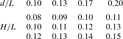
Reference Lubin, Vincent, Abadie and Caltagirone2006), we used the values presented in table 1 to generate plunging breaking waves, ranging from weak to energetic events. The real air and water physical properties are used. The physical parameters are summarised in table 2.
Initial values for the wave steepness
 $H/L$
and the dispersion parameter
 $d/L$
for the 12 different 3D plunging breaking waves simulated in this paper. According to previous numerical simulations (Lubin et al.
Reference Lubin, Vincent, Abadie and Caltagirone2006), for a given dispersion parameter value, the greater the wave steepness is, the stronger the plunging breaking event will be. The configuration with
 $H/L=0.13$
and
 $d/L=0.13$
is mainly discussed.

Physical parameters used for all the 3D numerical simulations.

The 3D numerical domains are discretised into
 $1024\times 500\times 200$
non-regular Cartesian cells (more than 100 million mesh grid cells), and partitioned into 1024 subdomains (one processor per subdomain). The grid is evenly distributed in longitudinal and transverse directions, giving a mesh grid resolution of
 ${\rm\Delta}x={\rm\Delta}y=10^{-4}~\text{m}$
. In the vertical direction, the grid is clustered with a constant grid size
 ${\rm\Delta}z=10^{-4}~\text{m}$
below
 $z=3\times 10^{-2}~\text{m}$
. A non-regular grid resolution is used above, with a maximum mesh grid size at the top of the numerical domain. This is further referred to as the L1 configuration (table 3) using the reference grid (RG) (table 4). At the initial time of the simulation, the interface and water velocity field from the wave are obtained from the linear theory and the air is at rest (Lubin et al.
Reference Lubin, Vincent, Abadie and Caltagirone2006). Hydrostatic pressure is initialised in the whole numerical domain. The computing time was approximately 24 h, with 1024 cores, for a simulated time of 0.88 s.
Numerical configurations used in the present work. The numerical domains are one wavelength long and the scale effects are discussed in § 3.5, with wavelength increasing from 0.10 to 0.20 m. The effect of the width of the numerical domain is also discussed by widening the configuration L1 to L1W.

Mesh grid densities used in the present work with the L1 configuration, from 1.28 to 0.819 billion mesh grid points.

Breaking waves are known to entrain a volume of air that evolves into a bubble size distribution, which ranges in size from tens of micrometres to centimetres. Deane & Stokes (Reference Deane and Stokes2002) studied the bubble distribution and the fragmentation process of the air cavity entrapped by breaking waves, from the jet impact to the collapse of the main air cavity. They showed that bubbles larger than 1 mm were subjected to fragmentation, whereas smaller bubbles were stabilised by surface tension forces and did not fragment. In order to be able to simulate air inclusions down to 1 mm size, we have to consider a mesh grid resolution of the order of
 $10^{-4}~\text{m}$
(L1 configuration detailed in table 3), keeping in mind that this is still not sufficient. In order to keep a reasonable time for the computations, we have to reduce the wavelength to
 $L=0.1~\text{m}$
. Numerical tests are shown in § 3.5 to evaluate the scale effects when increasing the wavelength, considering the numerical configurations given in table 3.
We further mainly detail the process of vortex filament generation and describe the plunging breaking wave simulated with
 $H/L=0.13$
and
 $d/L=0.13$
. In order to discuss the capacity of the numerical tool to describe accurately such fine details, we also present in § 3.5 a mesh grid analysis using four different mesh grid resolutions ranging from
 $4\times 10^{-4}$
to
 $0.5\times 10^{-4}~\text{m}$
, the latter requiring almost a billion mesh grid points. The number of processors used to perform this numerical analysis is given in table 4.
3. The mechanism of vortex filament generation
3.1. Preliminary analysis
As it approaches the beach, the propagating wave changes form, owing to the decrease in water depth, and its shape loses its symmetrical aspect. Once the front face of the wave steepens and becomes almost vertical, a jet of water is projected forwards from the crest of the wave. When the tongue of water free-falls forwards into a characteristic overturning motion, following a nearly ballistic trajectory, a tube of air is enveloped, generating a first large-scale aerated vortex. This pocket of air is entrapped and rotates at speed due to the high circulation flow of water surrounding it. The plunging jet closes over the air when it finally hits the wave face at the plunge point. The jet re-enters the water after impact, forcing up a second jet, called splash-up. This splash-up can rise higher than the original wave.
In rare documentary footage and in pictures showing breaking waves filmed from underwater, we identified some spinning aerated filaments under the impact zone. When analysing the existing films and pictures, some characteristic features of these well-defined hollow vortex filaments, also referred to as ‘coils’ by casual observers, could be detected. The fine coherent structures were fully 3D vortical tubes, like vortex filaments elongated in the main flow direction. The filaments were seen to occur only under plunging breaking waves, connecting the splash-up and the main tube of air. The generation mechanism and evolution of the vortex filaments is obviously a localised process remaining very close to the impact zone, and thus clearly seemed independent of water depth. We observed that these vortex filaments initiated when the tip of the jet touched the forward face of the wave. The filaments were then stretched from one end, following the rising splash-up, while the other end was wrapped around the main aerated cavity. The vortex filaments were observed to entrain large quantities of air funnelling inside the structures. The rotating structures appeared to start as large vortex tubes thinning with time and at times collapsing in bubbly filaments, while some of the detected structures could be very thin from the beginning. The vortex filaments often seemed to be regularly distributed and evenly spaced along the spanwise direction, while we found the downstream extremities of some vortex filaments to interact with each other and form larger vortex filaments. Sometimes, we had the chance to see some vortex filaments coiling, braiding or interlacing aesthetically. Even if no length nor time scales could be estimated from the existing materials, it was obvious that a large range of sizes and durations could be noticed. Nevertheless, the lifespan of the filament was closely linked to that of the main tube of air generated by the plunging crest of the wave. No preferred direction of rotation could also be identified. Some of the vortices were seen spinning in the same direction, while some neighbouring filaments rotated in the opposite direction.
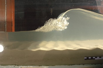
It was not clear from the pictures and film footage what the exact mechanisms responsible for the generation and evolution of the vortex filaments were. We could see the aerated filaments, but both extremities were often not visible owing to the chaotic motion of the flow in this highly aerated region, which was obscured by bubbly clouds. To date, very few experimental observations have been made in laboratories detailing these structures, though one photograph was found after we finished writing this article (figure 2). Some experimental works were also found to have been able to reproduce these vortex filaments, such as figure 3.11 of Lamarre (Reference Lamarre1993), figure 2(b) of Rojas & Loewen (Reference Rojas and Loewen2010) and figure 3(a) of Blenkinsopp & Chaplin (Reference Blenkinsopp and Chaplin2011).
Plunging breaking wave generated in the M2C Caen wave flume, revealing some tiny aerated vortex filaments. The black-and-white rule visible in the bottom right corner gives an idea of the dimensions (the large rectangles are 5 cm long and the small rectangles are 1 cm long). Picture used with kind permission of Dr Dominique Mouazé, University of Caen.

It is interesting to note that the vortices only appeared once in such detail (BBC 2009), despite filming more than 10 waves in Pohnpei (Micronesia) in April 2008 (Huw Cordey, personal communication). So how and where does it all start? What happens to the filaments clearly needs to be further investigated using high-resolution numerical simulations. An early citation of the BBC video can be found in Brucker et al. (Reference Brucker, O’Shea, Dommermuth and Adams2010), but no analysis was provided. Plunging breaking waves were numerically simulated to deduce the mechanisms responsible for the triggering of the swirling motion at the plunge point, their evolution and interactions, and the induced air entrainment.
3.2. Generation of the vortex filaments
Unless otherwise indicated, all length, time and velocity scales herein are normalised by the wavelength,
 $L$
, and characteristic time scale,
 $\sqrt{g/L}$
, respectively.
Usually, the most appropriate way to identify a vortex is to plot the instantaneous streamlines or vorticity contours. However, when the flow patterns are very complicated, vorticity contours alone cannot provide clear information. Thus, we choose to identify and trace the motions of vortex filaments and their evolutions in space and time using the
 $Q$
-criterion, introduced by Hunt, Wray & Moin (Reference Hunt, Wray and Moin1988) for coherent structure eduction, where
 $Q$
is the second invariant of the velocity gradient tensor (Jeong & Hussain Reference Jeong and Hussain1995). The
 $Q$
-criterion is defined as the balance between the rotation and strain rates. Having identified the aerated vortex filaments under the impact zone, it is expected that coherent hydrodynamical structures coincide with these areas. The distribution of positive values of the
 $Q$
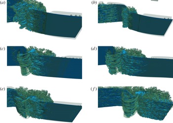
-criterion isolate areas where the strength of rotation overcomes the strain, thus identifying the location, direction and shape of the vortices. In figure 3, the vortex filaments are visualised under some plunging breaking waves. Two weak plungers are shown in figure 3(a,b). The overturning jets entrap a smaller tube of air, compared to stronger plunging breaking waves (figure 3
c–f). The lifespan of this aerated cavity is very short, as it appears to dislocate very rapidly in both cases. So, no vortex filament is observed, rather bubble plumes rotating in a large horizontal bore.
Examples of vortex filaments generated for some of the 3D breaking waves simulated in this paper (L1 configurations). (a,b) Two weak plunging breakers where no vortex filament is observed: (a)
 $H/L=0.10$
,
 $d/L=0.17$
; (b)
 $H/L=0.11$
,
 $d/L=0.20$
. (c–f) Plunging breakers where vortex filaments occur: (c)
 $H/L=0.10$
,
 $d/L=0.10$
; (d)
 $H/L=0.11$
,
 $d/L=0.13$
; (e)
 $H/L=0.12$
,
 $d/L=0.17$
; ( f)
 $H/L=0.13$
,
 $d/L=0.20$
.

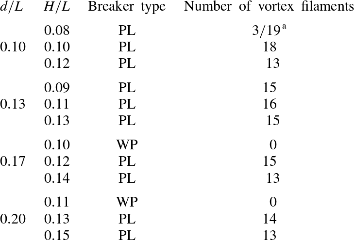
Table 5 summarises the number of vortex filaments that we observe from our simulations, as a function of the breaker type. Two breaking waves are identified as weak plunging breakers, which could be the limit between the plunging breaker and the spilling breaker. A small jet is still clearly visible from the crest of the breaking wave and impacts on the very upper part of the face of the wave. A spilling breaking wave involves a much more complex combination of wave propagation and vorticity generation based on perturbations appearing on the steepening face of the wave (Duncan et al.
Reference Duncan, Qiao, Philomin and Wenz1999). We consider that the grid refinement we use is not sufficient enough to be able to capture the mechanisms responsible for the generation of a ‘pure’ spilling breaking wave and surface tension is neglected in our simulations. It can be clearly deduced from table 5 that the vortex filaments are not a function of the breaker intensity. For a given dispersion parameter
 $d/L$
, the breaker intensity increases with the steepness of the wave
 $H/L$
. The most intense breakers are found at low dispersion parameter values and the steepest waves. One of the simulated waves (
 $H/L=0.08$
and
 $d/L=0.10$
) shows fewer vortex filaments. This less intense plunging breaker required a finer mesh grid density (FG) to display vortex filaments.
Counts of vortex filaments observed as a function of the breaker type: WP, weak plunging; PL, plunging breaker.
 $^{\text{a }}$
Using the RG grid, only three vortex filaments can be observed, while using the FG grid, more structures can be identified.

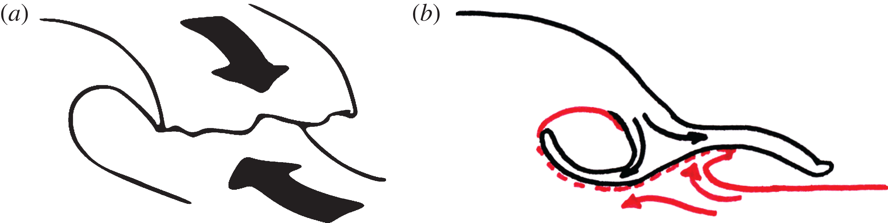
Many investigators (e.g. Kiger & Duncan Reference Kiger and Duncan2012) analysed in detail the splash-up generation and plunging jet re-entry in the forward face of the wave. It was shown that the jet does not penetrate, regardless of the position of the plunge point or the angle between the falling crest and the front face of the wave. It was also numerically confirmed that the jet of water was almost totally reflected when it hit the front face of the breaking wave (Abadie Reference Abadie1998; Yasuda et al. Reference Yasuda, Mutsuda, Mizutani and Matsuda1999; Dalrymple & Rogers Reference Dalrymple and Rogers2006; Lubin et al. Reference Lubin, Vincent, Abadie and Caltagirone2006; Landrini et al. Reference Landrini, Colagrossi, Greco and Tulin2007). Strong shear is generated due to the falling jet, moving forwards and downwards, impacting and entering the forward face of the wave, moving backwards and slightly upwards (figure 4 a). The tongue of water first hits the front face of the breaking wave and creates a notch. From this point, the tongue of water separates, as the two adverse flows of water meet. One part of the liquid forms the upper part of the splash-up, while the other goes backwards around the main pocket of entrapped air where a considerable topologically induced circulation takes place (Iafrati Reference Iafrati2011). Therefore, as sketched in figure 4(b), a line of discontinuity is found in the velocity field where the two opposing flows meet. This was discussed in detail by Peregrine (Reference Peregrine1981), who tried to develop a simple model of the flow after the plunging jet impact, and Watanabe et al. (Reference Watanabe, Saeki and Hosking2005).
(a) Sketch of the free-falling jet showing the adverse flows at the plunge point, prior to the impact. (b) Sketch of the colliding jet with the flow separation: downstream of the plunge point, the main tube of air is entrapped, while the splash-up is growing upstream. The arrows represent the opposing flows meeting and separating, creating a line of discontinuity.

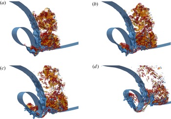
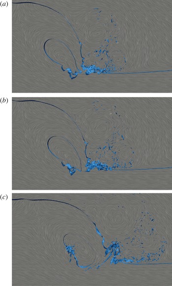
The vortex filament generation is a very transient phenomenon, occurring in less than a second. In figures 5 and 6 and supplementary movies 1 and 2 (available at http://dx.doi.org/10.1017/jfm.2015.62), a time-lapse sequence details the appearance of two vortex filaments.
Sequence of pictures presenting the evolution of two vortex filaments, from the touchdown of the plunger to the beginning of the splash-up generation, for
 $H/L=0.13$
and
 $d/L=0.13$
(L2 configuration). The vortex filaments are isolated in a 3D strip extracted from the whole numerical domain for a clearer identification of the structures. The free surface is identified with the isocontour of the phase function
 $C=0.5$
(in blue). The isocontours of the axial vorticity are calculated in an axis
 $x^{\prime }$
tilted
 $50^{\circ }$
from the horizontal axis
 $x$
(
 ${\it\omega}_{x^{\prime }}=700~\text{s}^{-1}$
in red and
 ${\it\omega}_{x^{\prime }}=-1000~\text{s}^{-1}$
in orange). The whole generation process is also shown in supplementary movies 1 and 2.

Sequence of pictures presenting the evolution of two vortex filaments, from the touchdown of the plunger to the beginning of the splash-up generation, for
 $H/L=0.13$
and
 $d/L=0.13$
(L2 configuration). The vortex filaments are isolated in a 3D strip extracted from the whole numerical domain for a clearer identification of the structures. The free surface is identified with the isocontour of the phase function
 $C=0.5$
(in blue). The line integral convolution, calculated in the 2D plane
 $(xz)$
, is displayed. The celerity of the initial wave is subtracted from the longitudinal velocity component to be in a frame of reference moving with the wave. The whole generation process is also shown in supplementary movies 1 and 2.

The tip shape of the plunger is neither a straight line nor a sharp edge (see figure 7 of Watanabe et al. (Reference Watanabe, Saeki and Hosking2005) and figure 4 a). It is commonly observed that the tongue of water ejected from the wave crest stretches and its tip fragments into droplets as it free-falls down, thereby exhibiting an irregular profile. When the jet of water collides with the wave face, the plunge location is not a thin line of contact but the tumultuous impact of a mass of water (figure 5 a). When the jet impinges on the face of the wave, it eventually creates a line of craters upstream from the plunge point, at the toe of the notch, which will further develop into the splash-up. The craters do not penetrate deeply, but expand due to the adverse flow from the forward face. The craters are deformed as they grow because of the increasing pressure between the colliding jet and the face of the wave. We observe an upward and forward motion of the lateral and upstream walls of the craters, while the bottoms move slightly backwards and downwards (figure 6 a) inclining the craters. Then, the craters begin to fold in on themselves, so the lateral walls begin a slanted backward motion creating wrinkles, initiating vorticity. The back of the plunging jet is observed to bend, so it now starts to move upwards and forwards at some point of the free surface to eventually close over the craters, creating cavities (figure 6 b). The lateral and downstream walls join together to entrap air. The walls of the craters are creased, with upward motion at the edges and downward motion at the bottoms. The folding-in motion of the craters on themselves is the seed of the vortical motion of the cavities.
Now, small aerated pockets are created. The obliqueness of these cavities is found to be determined in the very early stages of the process (approximately
 $50^{\circ }$
found from all the simulated configurations). The notch at the impact creates an angle responsible for the tilting of the nascent cavities (figure 5
b). As the liquid in the jet clearly separates, the splash projects forwards from the impact point. The upper parts of the aerated pockets are moving upwards, while the bottoms are pulled by the downdraught created along the line of discontinuity. This is clearly displayed in figure 6(c), where the streamlines delimit the saddle point. The vortex filaments appear from the cavities, which are then elongated, undergoing a stretching and intensification process in the strain region between the spanwise rotating tube of air and the developing splash-up (figure 5
b,c). The vortex filaments now develop into 3D streamwise coherent structures. The upstream ends remain attached to the generation points at the upper surface of the splash-ups, while the downstream ends are connected to the main tube of air (figure 5
d).
The rotating structures are thus clearly identified as soon as the jet enters the forward face of the wave. The vortex filaments are found to be located at the exact boundary between the water from the impacting jet and the water from the forward face of the wave, along the line of discontinuity in the strain region. During the splash-up evolution phase, a regular pattern can be observed with the development of the streamwise coherent vortices (figure 3). However, we do not identify any preferred direction of rotation from our numerical results, as already mentioned in the preliminary analysis. Indeed, at the early stage of the impact, vorticity is due to the development of the craters, whose shapes are highly irregular. Moreover, once the spiral motion of a developing filament has started in one direction, it tends to entrain and merge with the surrounding air pockets and bubbles, and interact with other neighbouring filaments. We could often see some structures combining to form one larger filament.
The plunging jet has a rough aspect on its back and under its extremity due to the small disturbances that grow during the fall (figure 5 a). Some longitudinal depressions are also observed on the back of the plunging jet, which correspond to the scars investigated by Watanabe et al. (Reference Watanabe, Saeki and Hosking2005) and Saruwatari et al. (Reference Saruwatari, Watanabe and Ingram2009). These local surface patterns are expected to be linked to the striations or the fingers detailed respectively by Longuet-Higgins (Reference Longuet-Higgins1995) and Narayanaswamy & Dalrymple (Reference Narayanaswamy, Dalrymple and Smith2002). The longitudinal distribution of the vortex filaments has been observed to be correlated with the striations visualised on the back of the impinging jet, the cavities being the main source of aeration of the vortex filaments when they first appear. The scars then lead to the formation of some bumps on the back of the plunging jet (figure 5 b,c), which is an early stage of disintegration of the free-falling jet (Longuet-Higgins Reference Longuet-Higgins1995). These bumps hit the water surface and cause some more pockets of air to be carried underwater and towards some vortex that is in formation (figure 5 d). When entrained in the water, these new pockets of air are flattened by the impact and are gradually stretched as they approach the line of discontinuity.
Figures 5(d) and 6(c) show that the upstream end of the vortex, or its ‘mouth’, is opened at the extremity of the developing splash-up. The downstream end is stretched, entrained towards the horizontal tube of air and wraps around it.
3.3. Comparison with shear flows
Some discussion should be provided about similar vortical structures encountered in shear flows. Some longitudinal vortices exist between 2D von Kármán vortices generated in the wake of a circular cylinder (Williamson Reference Williamson1996; Wu et al. Reference Wu, Sheridan, Welsh and Hourigan1996; Henderson Reference Henderson1997). A saddle point is induced by the stretching of two counter-rotating spanwise vortices, responsible for the occurrence of 3D vortex loops, similar to those found in a mixing layer.
What we find under breaking waves is very similar to the 3D streamwise vortices in a plane shear layer, as described by many authors (Neu Reference Neu1984; Bernal & Roshko Reference Bernal and Roshko1986; Lasheras, Cho & Maxworthy Reference Lasheras, Cho and Maxworthy1986; Ashurst & Meiburg Reference Ashurst and Meiburg1988; Lasheras & Choi Reference Lasheras and Choi1988; Fritts, Isler & Andreassen Reference Fritts, Isler and Andreassen1994; Andreassen et al. Reference Andreassen, Hvidsten, Fritts and Arendt1998; Fritts, Arendt & Andreassen Reference Fritts, Arendt and Andreassen1998). In a shear layer flow, the primary KH instability develops first, leading to the formation of an almost 2D array of spanwise vortex tubes, whose axes are perpendicular to the streamwise direction. The streamwise vortex structure has been proved, experimentally and numerically, to originate from an internal instability of the primary vortices. Then, in addition to the primary KH instability, a secondary instability appears. Owing to the strain field created between the evolving spanwise vortices, the perturbation grows as it is stretched, resulting in the formation of well-organised smaller vortex tubes whose axes are aligned with the principal direction of the positive strain field. The large spanwise rolls are connected to each other by the streamwise filaments (Neu Reference Neu1984; Fritts et al. Reference Fritts, Isler and Andreassen1994). Andreassen et al. (Reference Andreassen, Hvidsten, Fritts and Arendt1998) and Fritts et al. (Reference Fritts, Arendt and Andreassen1998) presented an analysis of the vorticity dynamics for a breaking internal gravity wave, based on a 3D high-resolution numerical model. Initial convective instability generates a series of intertwined vortex loops, linking continuously to the spanwise vortices due to stretch and intensification. Lasheras et al. (Reference Lasheras, Cho and Maxworthy1986), Lasheras & Choi (Reference Lasheras and Choi1988) proved that the plane turbulent shear layer is also composed of a secondary streamwise, coherent vortical structure, which superimposes onto a primary spanwise one.
Some differences can be highlighted between the vortex filaments observed under the breaking waves and the streamwise structures found in shear layer flows. In the latter case, the streamwise vortices are found to arise from a secondary instability between formed spanwise vortices. Then, the streamwise vortical structures are always observed first to form in the braids between the spanwise vortices and then to propagate into their cores (Lasheras et al. Reference Lasheras, Cho and Maxworthy1986). In our case, the triggering mechanism driving the transition to a 3D flow slightly differs. Each filament is individually generated from the plunge point, owing to the rotation of a cavity entrapped between the free-falling jet and the forward face of the wave. Then, the structure develops into a vortex filament through a stretch and intensification process in the strain region located between the main aerated cavity and the developing splash-up, analogous to what is observed in shear layer flows. We do not notice loops, or bending, or counter-rotating vortices. The extremities of the vortex filaments have been seen to be connected: one end is attached to the main tube of air and wraps around it, and the other end is opened at the free surface, at the upper part of the splash-up. Moreover, aeration of the vortex cores make the filaments hollow.
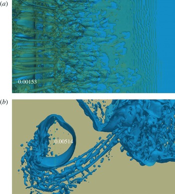
(a) The average diameter of the vortex filaments is
 $0.00153~\text{m}$
, while, for comparison, (b) the average diameter of the main aerated pocket of air is
 $0.00514~\text{m}$
. The vortex envelopes are visualised with
 $Q=1$
isosurfaces (in green) and the free surface is identified with the isocontour of the phase function
 $C=0.5$
(in blue). The wave is breaking from the left to the right (
 $H/L=0.13$
and
 $d/L=0.13$
, L2 configuration).

Our vortex filaments thus also differ from the vortex loops mentioned by Watanabe et al. (Reference Watanabe, Saeki and Hosking2005). Their results detail the formation of streamwise vortices occurring several times between consecutive co-rotating vortices generated by a sequence of splash-ups. Watanabe et al. (Reference Watanabe, Saeki and Hosking2005) assumed that the mechanisms responsible for the formation of the vortex loops are analogous to those described in KH instability. A continuous spanwise vortex sheet is identified at the plunge point and an instability in the saddle region leads to a rapid growth of spanwise perturbations. The vortex sheet is then stretched, and extremities are bent, forming the continuous streamwise counter-rotating vortices. This may be due to the coarse mesh grid resolution or to some assumptions made by Watanabe et al. (Reference Watanabe, Saeki and Hosking2005), such as single-phase flow simulations (no aeration taken into account) without strong surface distortions. We also simulated a single breaking event in a periodic domain, while Watanabe et al. (Reference Watanabe, Saeki and Hosking2005) simulated regular waves breaking one after another. So, each wave interacts with the remaining vorticity left by the previous breaking wave, which affects the overall vorticity field.
3.4. Temporal and spatial evolution of the vortex filaments
In this section, some quantitative descriptions and general trends are presented. The average diameter of the vortex filaments is not easy to determine, as it depends on the threshold used to define the vortex core. Whether we should measure the size of the air entrapped in the core of the filaments or the envelope for a given
 $Q$
-criterion isocontour is not an easy question. We show in figure 7 the measurement of an average vortex filament at a given time, which is
 $0.00153~\text{m}$
based on the
 $Q$
-criterion isocontour used to visualise the vortex filaments. The average diameter of the aerated core is one-third to one-quarter of the vortex diameter, which is approximately
 $4\times 10^{-4}~\text{m}$
. For comparison, we also give the average diameter of the main air pocket entrapped by the impinging jet when the wave breaks (
 $0.00514~\text{m}$
). The azimuthal velocity is approximately
 $0.3~\text{m}~\text{s}^{-1}$
for the large air pocket, while we find an azimuthal velocity of
 $0.275~\text{m}~\text{s}^{-1}$
for the vortex filament, the velocities being measured at the locations shown in figure 7.
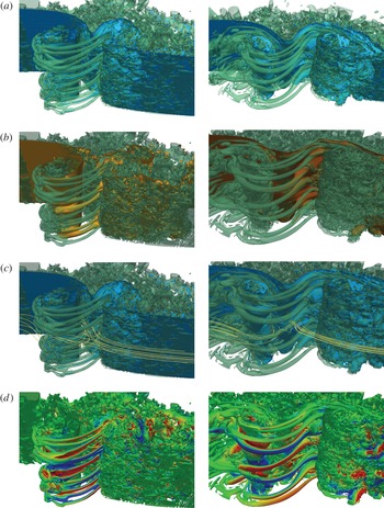
Figure 8 depicts the distribution of the vortex filaments in the flow, at
 $t=0.17~\text{s}$
and
 $t=0.24~\text{s}$
. The main concern, when using the
 $Q$
-criterion alone, is obviously the setting of the threshold. To investigate the dynamics of the coherent structures in more detail, the vortex filaments are shown in figure 8 using a rather loose criterion
 $Q=1$
combined with the free-surface topography, the streamlines and some scalar quantities, as they evolve in space and time. If higher
 $Q$
-criterion values are used, only few details disappear in the regions where the water flow is associated with weak local velocity fluctuations, while the vortex filaments remain distinctly delineated, indicating a strong vortical motion. Further discussion of coherent structures is therefore based on the use of
 $Q=1$
.
Evolution of the coherent vortical structures underneath the plunging breaking wave at
 $t=0.17~\text{s}$
(left column) and
 $t=0.24~\text{s}$
(right column), for
 $H/L=0.13$
and
 $d/L=0.13$
(L1 configuration). The coherent vortex filaments are educed using the
 $Q$
-criterion (Hunt et al.
Reference Hunt, Wray and Moin1988). The vortex envelopes are visualised with the positive
 $Q=1$
isosurfaces (in green). (a) The free surface is identified with the isocontour of the phase function (in blue), showing the air entrainment. (b) The pressure isocontour (
 $p=0.7~\text{N}~\text{m}^{-2}$
, with the reference
 $p=0$
located at the free surface) illustrates the low pressure inside the vortex filaments. (c) Streamlines show spiralling flow around and inside the fine elongated vortex filaments. (d) The colour scale on the isosurfaces of
 $Q=1$
refers to the local value of the spanwise velocity. Regions associated with positive spanwise velocity are in red, negative in blue. The whole dynamic is also shown for the free surface in supplementary movie 3.

The structures are observed to be persistent in time; they do not disappear nor do new ones appear as the wave breaks. A regular distribution of the vortex filaments can be seen in figure 8, with structures that are clearly distinct from adjacent ones and well organised. The fine elongated structures form a rib cage, linking the splash-up to the main pocket of air. Air entrainment does indeed coincide with the coherent structures educed from the
 $Q$
-criterion (figure 8
a), as it is drained inside the vortex filaments. The size of the filaments are observed to be linked to the size of the pockets of air entrapped at the beginning of the process (see supplementary movies 1 and 2).
It is evident from figure 8(b) that the vortex filaments are low-pressure regions. Once the vortex core forms, air is entrained and the pressure inside the filaments becomes lower than the value of the surrounding fluid. This is in accordance with the general observation that pressure has relatively low values in the centre of a region of strong rotational fluid motion. It can be mentioned that the pressure criterion corresponds with the
 $Q$
-criterion for each aerated vortex tube. The
 $Q$
-criterion that is chosen in the present study shares some properties with both the vorticity and the pressure criterion.
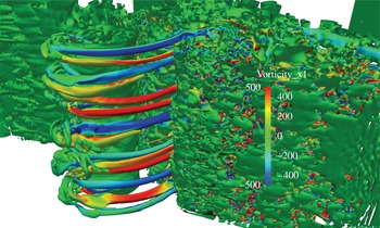
Evidence of the spiralling flow around the envelopes of the vortices is clearly shown in figure 8(c). The streamlines detail the swirling motion and the discontinuity, as the adverse upstream and downstream flows meet at impact. Figures 8(d) and 9 confirm the observations that the vortices exhibit no preferred direction for the swirling motion nor any specific alternating pattern.
Picture showing the axial vorticity to indicate the orientations of the rotating motions of the vortex filaments. The vortex envelopes are visualised with the positive
 $Q=1$
isosurfaces (in green), and coloured with the isocontours of the axial vorticity (
 ${\it\omega}_{x^{\prime }}=400~\text{s}^{-1}$
in red and
 ${\it\omega}_{x^{\prime }}=-400~\text{s}^{-1}$
in blue). Here
 $H/L=0.13$
and
 $d/L=0.13$
; L1 configuration.

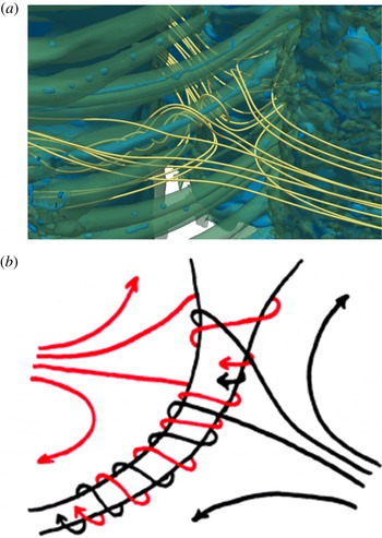
Figure 10 details how the adverse flows meet and wrap around the vortex filaments, rotating from the mouth towards the interior of the wave.
Streamlines detail spiralling around an aerated vortex filament: (a) close-up of figure 8(c) showing the intricate motion of the streamlines; (b) schematic depicting the swirling motion resulting from the impingement of the mass of water coming from the plunging jet (left) and the forward face of the wave (right) to form the vortex filament. The splitting of the bodies of water delimits a line of separation and creates the stretching of the filament.

The downstream ends of the vortex filaments are observed to be connected with the main tube of air. They are sometimes deformed and flattened, and often noticed to experience complicated entanglements. It has also been seen that the vortex filaments could be aerated as long as the mouth was still opened at the free surface. Some filaments have been observed to be gradually emptied of air, but the hydrodynamic coherent structures persisted in the flow and could sometimes suck air inside the core again, like a bathtub vortex. The numerical results presented in this paper can be easily compared to the underwater pictures shown in figure 1 and match all the observations detailed in § 3.1.
3.5. Scale effects and mesh grid sensitivity
Owing to the fact that all the previous analysis and description relies upon numerical results, some points should be addressed concerning the assumptions and choices made about wavelength, omission of surface tension and mesh grid resolutions.
Considering the smallest wavelength in our work (L1), our results could be affected by the absence of surface tension, which could have prevented the generation of the vortex filaments during the plunging jet impact. However, most recent studies neglected air entrainment and surface tension (Christensen & Deigaard Reference Christensen and Deigaard2001; Watanabe et al. Reference Watanabe, Saeki and Hosking2005; Christensen Reference Christensen2006; Landrini et al. Reference Landrini, Colagrossi, Greco and Tulin2007; Saruwatari et al. Reference Saruwatari, Watanabe and Ingram2009), and were limited to 2D numerical configurations (Iafrati Reference Iafrati2009, Reference Iafrati2011) or coarse 3D resolutions owing to the large numerical domains (Christensen & Deigaard Reference Christensen and Deigaard2001; Lakehal & Liovic Reference Lakehal and Liovic2011; Higuera, Lara & Losada Reference Higuera, Lara and Losada2013). In the present study, the mesh grid resolution is chosen to describe fine inclusions larger than 1 mm, to identify the main mechanisms involved in the generation of vortex filaments and to describe qualitatively their evolution in the flow. But running 3D numerical simulations at such a length scale, considering surface tension, is still a challenge. Indeed, several mesh grid points are necessary to compute precisely the free-surface curvature used to model surface tension. So considering the smallest inclusions encountered in our numerical simulations, taking surface tension into account, would lead to inaccurate behaviour and spurious velocities, even with almost one billion mesh grid points.
Deane & Stokes (Reference Deane and Stokes2002), considering experimental waves with a much larger wavelength (
 $L=2.3~\text{m}$
) than ours, showed that bubbles larger than the Hinze scale (1 mm radius) are subject to fragmentation by turbulent and sheared flow, whereas bubbles smaller than the Hinze scale are maintained by surface tension. So, at a scale smaller than the Hinze scale, where surface tension is large enough to prevent breaking up, the interfacial energy is balanced by the turbulent kinetic energy of the flow. Subsequently, the fragmentation process ceases.
Brochini & Peregrine (Reference Brochini and Peregrine2001) indicated that, at the shortest scales, the stabilising actions of gravity and surface tension dominate over the disrupting effect of turbulence. Song & Sirviente (Reference Song and Sirviente2004) also proved numerically the increasing role of surface tension, associated with a significant reduction in jet intensity and air entrapment. But using a wavelength
 $L=0.27~\text{m}$
, Iafrati (Reference Iafrati2009) noticed that, owing to the high Weber number of his numerical simulations, the surface tension contribution to the energy balance was found to be negligible, as also mentioned by Chen et al. (Reference Chen, Kharif, Zaleski and Li1999). Iafrati (Reference Iafrati2009) evaluated the energy associated with surface tension effects being less than 0.2 % of the initial energy content in his configuration (
 $\mathit{Re}=10^{4}$
,
 $\mathit{We}=100$
).
To evaluate the influence of the omission of surface tension, we show two configurations with doubled wavelengths from 0.1 to
 $0.2~\text{m}$
. We evaluate the Reynolds numbers of the initial waves, considering the initial quantities, and the Weber number as if surface tension was taken into account (
 $\mathit{Re}_{w}$
and
 $\mathit{We}_{w}$
), but assuming the effect of surface tension would be negligible. When we modify the initial wavelength and thus increase the numerical domain, the initial water depth and the initial wave height vary according to the wave steepness
 $H/L$
and dispersion parameter
 $d/L$
to achieve geometrical similarity. We do not satisfy kinematic similarity, as the Reynolds numbers are not constant. As Battjes (Reference Battjes1988) mentioned, the process of wave steepening, overturning and jet formation is essentially an irrotational motion. Even at the instant when the free-falling jet touches down on the lower face of the wave and forms a cavity, the motion is still irrotational (Battjes Reference Battjes1988). So the flow is expected to be driven by the Reynolds number only when the jet impingement induces the transition to strong rotational motions and turbulence is generated.
Gomez-Ledesma, Kiger & Duncan (Reference Gomez-Ledesma, Kiger and Duncan2011) presented an experimental study on the impact of a translating 2D transient jet on an initially quiescent liquid pool, mimicking a plunging breaker situation. The Reynolds numbers ranged between 6520 and 9754, whereas the Weber numbers considered were between 2.1 and 4.6. Some large volumes of air were shown to be entrained and a great number of bubbles were generated, owing to the collapse of the large air cavities. The jets were shown to penetrate into the pool, producing clouds of bubbles, entrained downstream and eventually observed to rise under the influence of buoyancy. Gomez-Ledesma et al. (Reference Gomez-Ledesma, Kiger and Duncan2011) indicated that higher translation speeds would have generated non-penetrating jet impacts, allowing the creation of larger upstream splash-ups as in a plunging breaker (Kiger & Duncan Reference Kiger and Duncan2012). We also considered the same Reynolds number (
 $\mathit{Re}_{j}$
) with respect to the subsequent plunging jet about to impact the forward face of the wave, leading to the generation of vortex filaments.
As presented in table 6, the Reynolds number of the plunging jet can be considered to be sufficiently large to assume that the process of air entrainment and vortex filament generation at the impact can be correctly described if surface tension is neglected in the L2 configuration. Looking at the two configurations, we checked that our results for the free-falling jets are in accordance with the approximation given by Drazen, Melville & Lenain (Reference Drazen, Melville and Lenain2008) for the vertical velocity of the toe at impact on the surface (
 $w_{j}=(2gh)^{1/2}$
, with
 $h$
defined as the height of the breaking region).
Initial and computed characteristics of the plunging breaking waves with the initial values of
 $H/L=0.13$
and
 $d/L=0.13$
, depending on the initial wavelength (left columns). The initial wave celerity
 $c_{w}$
, Reynolds number
 $\mathit{Re}_{w}={\it\rho}_{w}g^{1/2}L^{3/2}/{\it\mu}_{w}$
and Weber number
 $\mathit{We}_{w}=g^{1/2}L({\it\rho}_{w}/{\it\sigma})^{1/2}$
(as if surface tension were taken into account) are given. The simulated heights at breaking
 $H_{b}$
, plunging jet thicknesses
 $t_{j}$
before impacting the front face of the wave, the vertical velocities of the tips of the jets before impact
 $w_{j}$
, and the Reynolds number
 $\mathit{Re}_{j}={\it\rho}_{w}w_{j}t_{j}/{\it\mu}_{w}$
and Weber number of the plunging jets
 $\mathit{We}_{j}={\it\rho}_{w}w_{j}^{2}t_{j}/{\it\sigma}$
, with surface tension of water taken at
 ${\it\sigma}=0.075~\text{N}~\text{m}^{-1}$
, are shown in the right columns.

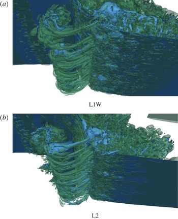
Figure 11 presents a qualitative comparison of the vortex generation obtained from the two numerical configurations presented in table 6. It can be clearly seen that approximately the same number of filaments is generated, their distribution and spacing along the spanwise direction being roughly the same. So, using the L2 configuration as a reference and assuming that surface tension can be neglected for this configuration, we can conclude that the configuration L1 with shorter wavelength is satisfactory compared to L2. If we can assume that surface tension would not have prevented the generation of the vortex filaments, we can however presume that surface tension would have prevented the fragmentation process of the aerated vortex filaments in both configurations.
Pictures showing the vortex filaments simulated with increasing initial wavelength from (a) to (b), for
 $H/L=0.13$
and
 $d/L=0.13$
. The vortex envelopes are visualised with the positive
 $Q=1$
isosurfaces (in green) and the free surface is identified with the isocontour of the phase function
 $C=0.5$
(in blue), showing the air entrainment.

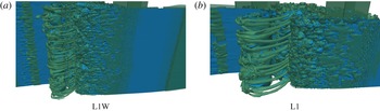
Keeping the width of the numerical domain constant and decreasing the initial wavelength from L2 to L1W does not affect the generation of vortex filaments, as observed in figure 11. To define the length scale, we then choose to focus attention on the Reynolds number. The study referred to a very large length scale (L3), at which surface tension is actually negligible. But in order to have a mesh grid resolution sufficient to describe correctly viscous and turbulent effects, the Reynolds number cannot be too high and this is why the fundamental wavelength is set to 10 cm. Moreover, in order to reduce the computational time, we thus choose to reduce the wavelength and neglect surface tension, so we can educe the formation of the vortex filaments with small-scale prototypical plunging breaking waves for different breaking intensities.
In order to verify the effect of the width of the numerical domain, we divide it by two from L1W to L1, as given in table 3. The pictures shown in figure 12 indicate that we approximately double the number of vortex filaments when doubling the width of the numerical domain. According to these comparisons, we can conclude that the mechanisms responsible for the vortex filaments are not a function of the wavelength, or of the width of the numerical domain.
Pictures showing the vortex filaments simulated with decreasing initial width of the numerical domain, from (a) to (b), for
 $H/L=0.13$
and
 $d/L=0.13$
. The vortex envelopes are visualised with the positive
 $Q=1$
isosurfaces (in green) and the free surface is identified with the isocontour of the phase function
 $C=0.5$
(in blue), showing the air entrainment.

A question arose when looking at previous work dedicated to exactly the same configuration (Lubin et al.
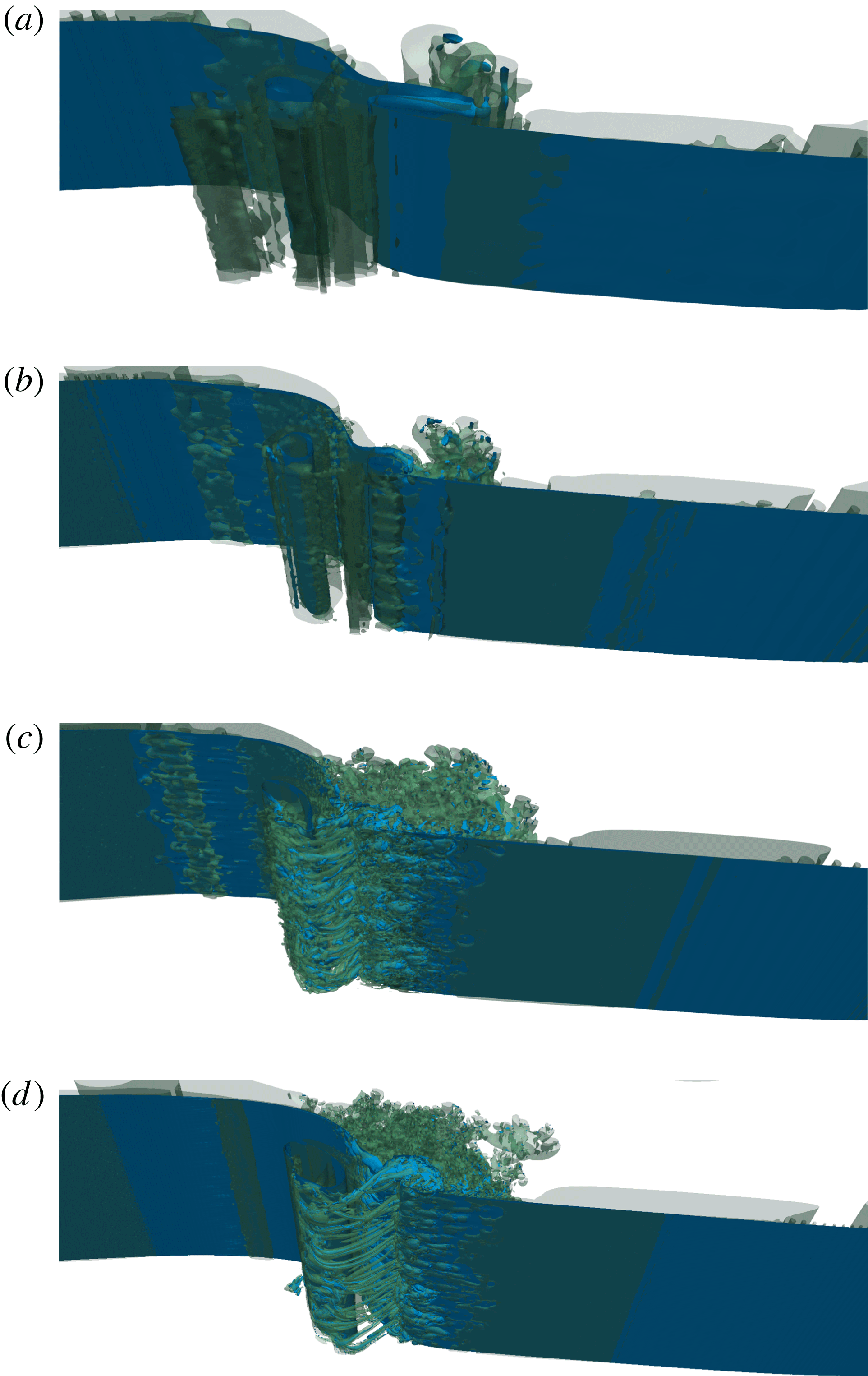
Reference Lubin, Vincent, Abadie and Caltagirone2006), where vortex filaments have never been observed. So, we also performed a mesh grid sensitivity, considering four mesh grid densities (table 2). To assess the convergence of our numerical results with grid resolution, we present in figure 13 a comparison of our simulations at a given time. This numerical test confirmed that the vortex filaments could not be seen by Lubin et al. (Reference Lubin, Vincent, Abadie and Caltagirone2006), considering the mesh grid density
 ${\rm\Delta}x\simeq {\rm\Delta}z={\rm\Delta}y=4\times 10^{-4}~\text{m}$
(CG grid). As expected, much less detail can be seen for air entrainment, and no vortex filaments are detected. The splash-up is much thicker and is projected much further as a long tongue of water. Fewer droplets are ejected in the air, the flow in the gas medium thus being less turbulent. Increasing the number of mesh grid points, to reduce the mesh grid density to
 ${\rm\Delta}x\simeq {\rm\Delta}z={\rm\Delta}y=2\times 10^{-4}~\text{m}$
(IG grid), did not allow a better description of the vortex filaments. Nevertheless, the splash-up is simulated with more details than previously, and is projected less far. Then, the finest mesh grid density (FG grid) allowed a better description of the aeration inside the vortex filaments. The structures are more clearly separated from each other and aeration has been observed to last longer in the core of the filaments, owing to a more accurate free-surface description. However, approximately the same number of filaments can be found when compared to the RG grid results. However, one case has been found to be sensitive to the mesh grid refinement, as identified in table 5.
Convergence study for four different mesh grid resolutions ((a) CG, coarse; (b) IG, intermediate; (c) RG, reference; (d) FG, fine (see table 4)) in the L1 configuration, with
 $H/L=0.13$
and
 $d/L=0.13$
. The vortex envelopes are visualised with the positive
 $Q=1$
isosurfaces (in green) and the free surface is identified with the isocontour of the phase function (in blue).

The interesting result of the CG and IG grids is the resulting flow, which is mainly 2D with two large spanwise vortical structures separated by a strain region, similarly to co-rotating vortices in a mixing layer. We do not observe any streamwise vortices or braids, as could be expected from what has been described concerning shear flows. So the numerical simulations do not capture any secondary hydrodynamic instability that could lead to the formation of well-organised streamwise counter-rotating vortices (Lasheras et al. Reference Lasheras, Cho and Maxworthy1986) or vortex loops (Watanabe et al. Reference Watanabe, Saeki and Hosking2005). The coarse grids used by Watanabe et al. (Reference Watanabe, Saeki and Hosking2005) should thus not be responsible for the differences observed between our observations.
3.6. Influence of the vortex filaments on the total energy dissipation
The total wave energy dissipation process is now investigated. According to (3.1), the dimensional kinetic, potential and total energies are
 $$\begin{eqnarray}\displaystyle \left.\begin{array}{@{}c@{}}E_{k}=\displaystyle \frac{1}{2}\displaystyle \iint {\it\rho}u^{2}\,\text{d}x\,\text{d}y,\\ E_{p}=\displaystyle \iint {\it\rho}z\,\text{d}x\,\text{d}y,\\ E_{t}=E_{k}+E_{p}.\end{array}\right\} & & \displaystyle\end{eqnarray}$$
The integrations are carried out over the whole domain, in the liquid part, with the bottom
 $z=0~\text{m}$
as the reference level for the calculation of the potential energy. We also define zero potential energy corresponding to a non-perturbed surface, and we normalise the values of the energies by the respective initial values (Chen et al.
Reference Chen, Kharif, Zaleski and Li1999; Lubin et al.
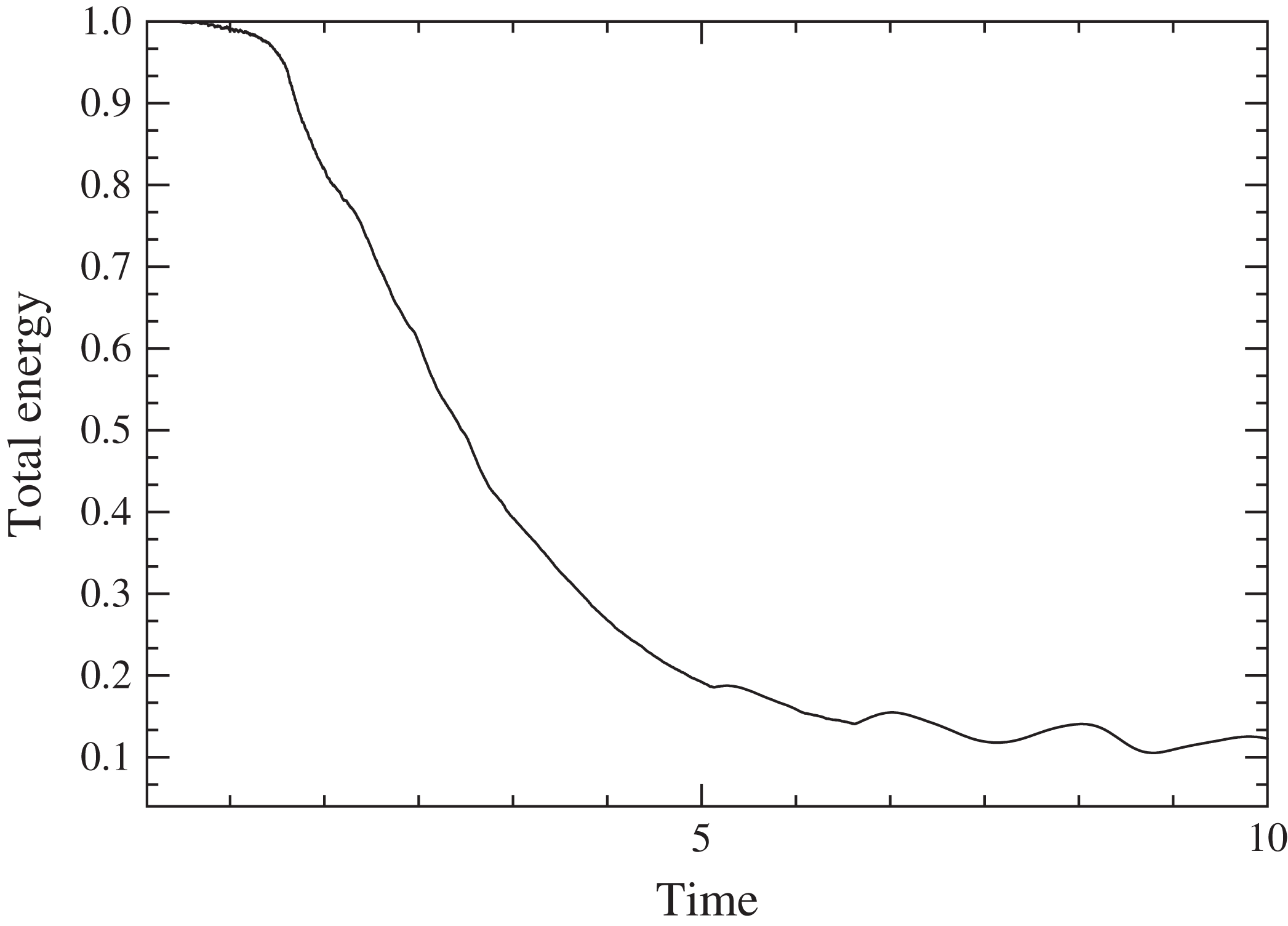
Reference Lubin, Vincent, Abadie and Caltagirone2006; Iafrati Reference Iafrati2009) and the time by the initial wave period. In figure 14, we plot the time evolution of the total energy of the wave, normalised by its initial value, for the case where
 $H/L=0.13$
and
 $d/L=0.13$
.
Time evolution of the total energy (non-dimensional quantities
 $t/T$
versus
 $E_{t}(t)/E_{t}(0)$
) for
 $H/L=0.13$
and
 $d/L=0.13$
.

Rapp & Melville (Reference Rapp and Melville1990) measured the turbulence generated by fully unsteady breaking waves in the laboratory. They found that approximately 90 % of the energy lost from the waves was dissipated within four wave periods, and that subsequently the kinetic energy decayed as
 $t^{-1}$
. Lamarre & Melville (Reference Lamarre and Melville1991) showed experimentally that the work done against buoyancy in entraining air could account for up to 50 % of the energy lost from the wave field. These results would suggest that air entrainment is a highly dissipative process and should therefore be taken into account when simulating or modelling breaking waves. Melville, Veron & White (Reference Melville, Veron and White2002) also proved that the turbulent kinetic energy decays with a
 $t^{-1}$
dependence for three types of breaker (spilling, weak plunging and plunging breakers), later confirmed by Drazen et al. (Reference Drazen, Melville and Lenain2008).
These experimental findings were successfully compared to some numerical works (Chen et al.
Reference Chen, Kharif, Zaleski and Li1999; Lubin et al.
Reference Lubin, Vincent, Abadie and Caltagirone2006; Iafrati Reference Iafrati2009; Lakehal & Liovic Reference Lakehal and Liovic2011). While Chen et al. (Reference Chen, Kharif, Zaleski and Li1999) and Iafrati (Reference Iafrati2009) simulated 2D breaking, including splash-up and air entrainment following the impact of the plunging jet, they found that 80 % of the pre-breaking wave energy was dissipated within three wave periods after breaking. It subsequently decayed as
 $t^{-1}$
, which is consistent with the experimental measurements. Unfortunately, Watanabe et al. (Reference Watanabe, Saeki and Hosking2005) did not evaluate the dissipation energy, so no comparison is possible. Lubin et al. (Reference Lubin, Vincent, Abadie and Caltagirone2006) showed a comparison between the time histories of the energy obtained by 2D and 3D calculations. Even if it was shown that 3D turbulence enhances energy dissipation, surprisingly, the differences between the 2D and 3D results were minor (
 ${<}5\,\%$
up to a half-wave period after the breaking event). Two-and-a-half periods after the breaking event, the difference in the energy contents of the 2D and 3D simulations was found to be 10 %.
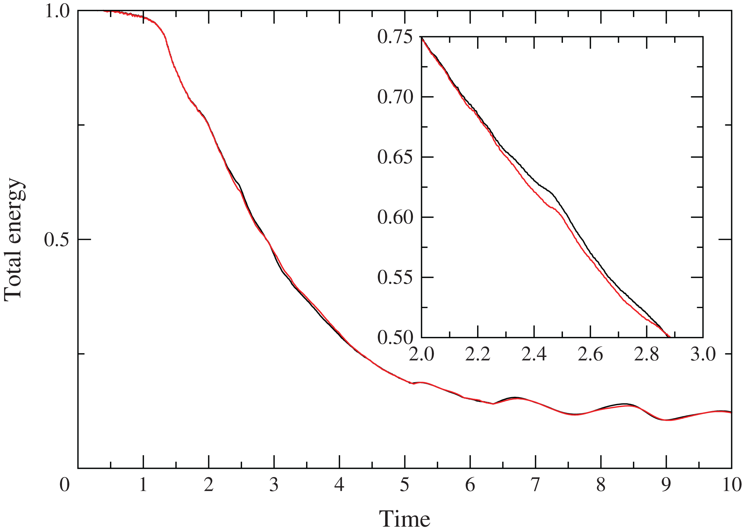
In the example displayed in figure 14, we can see that our detailed 3D simulation is in accordance with the previous findings. The same
 $t^{-1}$
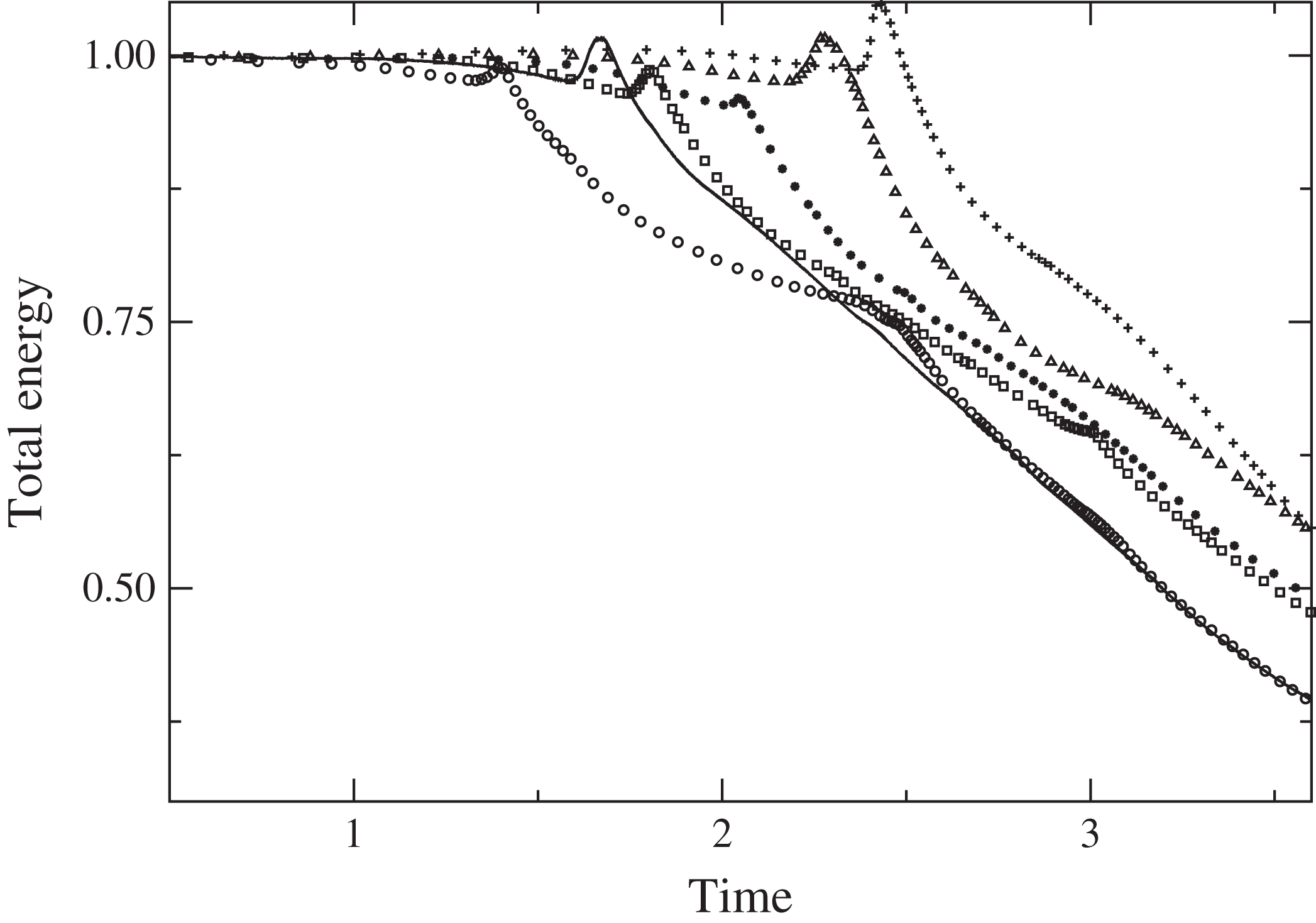
decay rate is also found. The most surprising feature is the similar total energy dissipation found for both CG and RG grids. Indeed, the two curves plotted in figure 15 match almost perfectly. Focusing on the vortex filaments described in this article, this would mean that the structures have no influence on the dissipation energy of the breaking wave. A coarse grid is sufficient to describe the largest eddies in the flow and to account for the correct decay rate of the total energy of the wave. The small size of the vortex filaments compared to the largest aerated cavities should be borne in mind (figure 7). This is also supported by the time histories drawn in figure 16, where we compare the total energy dissipation for different breaker intensities. It can be clearly seen that all the curves exhibit the same decay rate, even for the weak plunging case where no vortex filaments were observed (
 $H/L=0.10$
,
 $d/L=0.17$
). This is in accordance with the results presented by Melville et al. (Reference Melville, Veron and White2002), who found the same decay rate of the energy dissipation for the three breaker types.
Comparison of the time evolutions of the total energy (non-dimensional quantities
 $t/T$
versus
 $E_{t}(t)/E_{t}(0)$
), for the coarse (grey; red online) and reference (black line) grids. A zoom is shown to differentiate the two curves, which are almost superimposed. Here
 $H/L=0.13$
and
 $d/L=0.13$
.

Comparison of the time evolutions of the total energy (non-dimensional quantities
 $t/T$
versus
 $E_{t}(t)/E_{t}(0)$
): solid line,
 $H/L=0.14$
,
 $d/L=0.17$
;
 $+$
,
 $H/L=0.10$
,
 $d/L=0.17$
; ▵,
 $H/L=0.09$
,
 $d/L=0.13$
; ▫,
 $H/L=0.11$
,
 $d/L=0.13$
; ○,
 $H/L=0.12$
,
 $d/L=0.10$
;
 $\ast$
,
 $H/L=0.08$
,
 $d/L=0.10$
.

4. Conclusions
The scope of this paper is to highlight the existence of unusual vortical structures under breaking waves and investigate the mechanisms of their generation. The
 $Q$
-criterion has been an effective way of visualising the aerated vortex filaments while preserving the physical details. Several breaker intensities have been simulated to confirm the conditions of occurrence of the vortex filaments, their generation and their development.
The vortex filaments under breaking waves are detected to be individual streamwise vortical structures, undergoing a stretch and intensification process in the strain region between the spanwise tube of air entrapped by the impinging jet and the developing splash-up. The impacting jet generates craters, which will eventually fold in on themselves to create cavities. These pockets of air have been noticed to start rotating while their lateral and downstream walls come together to close the oblique cavities. The upper parts of the pockets are moving upwards and forwards, due to the splashing, while the bottoms are pulled backwards and downwards. The streamwise structures are then elongated, due to the shear in the saddle region.
The streamwise vortex filaments have been detected under plunging breaking waves only, with an upstream obliqueness of approximately
 $50^{\circ }$
. They have been shown to be independent of the breaker intensity. Their lateral distribution at generation seemed to be driven by the striations found on the back of the plunging jet. The total energy dissipation for different breaker intensities has been evaluated. We found no contribution due to the presence of the vortex filaments on the dissipation process.
Discussion about existing analogous streamwise vortical structures has been provided. The main difference is that we identified and explained how these vortex filaments were individually generated in the chaotic impact of a mass of water. The structures are observed to be aerated, as their mouth is attached to the free surface while the other end is linked to the main tube of air. We did not notice any bending at their extremities, nor continuous linking to neighbouring filaments to form loops (Watanabe et al. Reference Watanabe, Saeki and Hosking2005; Saruwatari et al. Reference Saruwatari, Watanabe and Ingram2009). The common point is the shear region in the saddle point, responsible for the stretch and intensification process of the filaments.
We explained that our choice of a short wavelength was governed by computational arguments, and we caution the reader about extrapolating our analysis to larger waves. Surface tension has been neglected in this work, so great care should be taken about the evolution of the air entrainment and the energy dissipation due to these fine structures. It has also to be remembered that capillary waves on short gravity waves could generate additional vorticity on the surface and thus cause another type of wave breaking (Longuet-Higgins Reference Longuet-Higgins1992). Capillary waves could also be responsible for some instabilities of the aerated vortex filaments and then lead to the early bursting of the structures.
Moreover, regular waves should be studied in future work. We simulated a single breaking event in a periodic domain, while Watanabe et al. (Reference Watanabe, Saeki and Hosking2005) simulated regular waves breaking one after another. So, we have to evaluate how each wave would interact with the remaining vorticity left by the previous breaking wave. The overall vorticity field should be more complex. For this reason, we also limited our discussion to the generation of vortex filaments and chose not to develop their interactions after wrapping around the main spanwise tube of air. No turbulent quantities have been estimated because the numerical configuration consists of a single breaker, so no mean velocity has been calculated to access the fluctuating quantities. An average velocity along the transverse axis could have been computed, but we did not consider this as equivalent to the time-averaged or phase-averaged velocity that we want to compute in the future when we will consider regular waves breaking one after the other. For this reason, we do not provide any discussion about any turbulent process or estimations (small-scale turbulence generation, turbulent dissipation, turbulent kinetic energy, etc.). Only instantaneous quantities are presented and discussed in this paper. Future work will be dedicated to address the generation of the other types of 3D structures encountered under breaking waves (obliquely descending eddies and downbursts). The generation of the striations on the back of the plunging jet is also a subject of future interest.
Acknowledgements
The authors wish to thank the Aquitaine Regional Council for financial support towards a 432-processor cluster investment, located in the I2M laboratory. This work was granted access to the HPC resources of CINES, under allocation 2013-x2012026104 made by GENCI (Grand Equipement National de Calcul Intensif), and PRACE-RI (Partnership for Advanced Computing in Europe Research Infrastructure), MAPAW project (Massively Parallel Navier–Stokes Solver for Air/Water environmental flows). Computer time for this study was also provided by the computing facilities at MCIA (Mésocentre de Calcul Intensif Aquitain) of the Université de Bordeaux and of the Université de Pau et des Pays de l’Adour. The authors would like to acknowledge helpful discussions with Professor R. Dalrymple, Dr Y. Watanabe and Dr F. Véron. Dr D. Mouazé, C. Bryan and M. Tipple are thanked for kindly allowing the use of photos. Their pictures and videos have been a true inspiration for this work.
Supplementary movies
Supplementary movies are available at http://dx.doi.org/10.1017/jfm.2015.62.